An Integrated regARIMA–HP Filter–CNN Framework with Attention Mechanism for Monthly Electricity Demand Forecasting

Abstract

Monthly electricity demand forecasts are often affected by outliers and moving-holiday effects. This study proposes a forecasting framework that integrates regression with ARIMA errors (regARIMA), Hodrick–Prescott (HP) filter decomposition, and a multi-branch convolutional neural network (CNN) with channel attention. The regARIMA model removes outlier and moving-holiday effects; the HP filter separates the adjusted series into trend and cyclical components; separate CNNs forecast these components; and the final forecast is reconstructed with moving-holiday correction. On the primary Changzhou dataset, the framework achieved the lowest two-year average RMSE (2.44), MAE (1.89), and MAPE (3.36%) and one of the highest R² values (0.91). In Guangzhou, it ranked second in the two-year averages of all four reported metrics. The top-ranked model retained the proposed X13-HP preprocessing and multi-scale CNN-attention core but added two bidirectional long short-term memory (Bi-LSTM) layers with self-attention. Per-comparison tests showed no statistically significant difference between this extended model and the proposed framework, and no multiplicity adjustment was applied. By contrast, a Bi-LSTM and self-attention model without the multi-scale CNN front end performed poorly. These results indicate that the main advantage of the proposed design lies in multi-scale convolutional feature extraction with channel attention, whereas recurrent depth alone is insufficient. The framework therefore provides accurate, stable, and structurally simpler forecasting.

1. Introduction

The safe and stable operation of the power system is essential to the normal functioning of the economy and society, and accurate electricity demand forecasting is a key prerequisite for this [1,2]. Based on the forecast time horizon, electricity demand can be categorized into long-, medium-, and short-term forecasts [3,4]. Long-term electricity demand forecasts form the basis for deploying future power generation plans, system upgrades, and grid expansion in power system planning [5]. Short-term demand forecasting is crucial for day-to-day market operations, providing decision-making support for market participants in risk assessment, bid optimization, and profit maximization [4]. Mid-term electricity demand forecasting is crucial for operational regulation of power systems, power generation scheduling, and formulation of electricity marketing strategies [1].

In recent years, electricity demand has grown rapidly with economic and social development—particularly with the rise of new electricity-consuming sectors such as data centers and electric vehicle charging [6,7]. At the same time, to mitigate the effects of climate change, electricity generation from renewable energy sources such as wind and solar power has grown rapidly [8]. However, due to the intermittent and volatile nature of renewable energy generation, the difficulty of dispatch in power systems has increased significantly, posing enormous challenges to the safe and stable operation of the power grid and further highlighting the importance of accurately forecasting medium-term electricity demand. Beginning in late 2019, the COVID-19 pandemic has altered short-term electricity consumption patterns and significantly changed the regularity of electricity demand fluctuations. These sharp fluctuations in electricity demand, caused by extreme weather events and sudden economic crises, have resulted in a number of outliers in electricity demand time series. These outliers undoubtedly have a significant impact on the construction of forecasting models. If outliers are not addressed effectively, a model’s predictive accuracy may be compromised.

Given that previous research on monthly electricity demand forecasting has yielded relatively limited results in handling outlier effects, this paper proposes a new hybrid forecasting model that accounts for their impact. The model first preprocesses raw electricity demand data using the regARIMA module of X-13ARIMA-SEATS (X13) to remove the effects of outliers and moving holidays. It then employs a Hodrick–Prescott (HP) filter to decompose the series, corrected for outliers and moving holidays, into trend and cyclical components. Subsequently, CNNs incorporating an attention mechanism are used to forecast each component series separately. Finally, the final forecast is obtained by reconstructing the component sequence forecasts and correcting for the moving-holiday effect. An application to electricity demand forecasting in Changzhou, China, shows that under the unified rolling protocol, the proposed model produced the fewest errors among the compared models.

1.1. Related Work

Early electricity demand forecasting primarily relied on statistical analysis methods to build predictive models. These methods mainly included the Autoregressive Integrated Moving Average (ARIMA) [9], Holt–Winters [10,11], and multiple regression models [12,13,14]. The main features of these methods are their simplicity and ease of implementation; they offer good forecasting accuracy when electricity demand changes are relatively stable. However, when electricity demand exhibits complex, nonlinear variations, the prediction errors tend to be relatively large. To effectively address the nonlinearity of electricity demand time series, machine learning-based forecasting methods have been applied. These methods primarily include tree-based models, such as Decision Tree Regression [15], Gradient-Boosted Decision Trees [16], Random Forest [17,18,19], Bayesian Additive Regression Trees [20], and kernel-based support vector regression (SVR) [21]. With the rise of deep learning technologies, neural network-based electricity demand forecasting models have become a focal point of research in academia and industry, leading to many of these models—for example, Chang et al. [22] proposed a method using weighted evolutionary fuzzy neural networks to forecast monthly electricity demand. A medium-term electricity forecasting model based on N-BEATS was proposed by Oreshkin et al. [23]. Chaturvedi et al. [24] validated the predictive performance of the long short-term memory (LSTM) network; Zhang et al. [17] evaluated the predictive performance of models such as LSTM and Gated Recurrent Units.

Many studies have found that relying on a single forecasting model does not effectively improve the accuracy of electricity demand forecasting. Consequently, many researchers have developed hybrid forecasting models to enhance accuracy by leveraging the complementary strengths of different models [25]. The development of these hybrid forecasting models has generally proceeded along two main lines. The first involves using the original electricity demand time series and combining different forecasting techniques to improve forecasting accuracy. Hong [26] proposed a hybrid forecasting model combining seasonal cyclical support vector regression with the chaotic artificial swarm algorithm. Cao and Wu [27] developed a seasonal electricity consumption forecasting model that combines the fruit fly optimization algorithm with support vector regression. Askari and Keynia [28] proposed a method for optimizing neural networks for medium-term electricity load forecasting using particle swarm and ant lion algorithms. Wu et al. [29] proposed a short-term electricity load forecasting model that uses the Cuckoo algorithm to optimize the parameters of the fractional ARIMA model. Jiang et al. [30] developed a monthly electricity consumption forecasting model that combines the fruit fly optimization algorithm with the Holt–Winters smoothing method. Hussein and Awad [31] constructed a power consumption forecasting model combining K-means clustering with Nonlinear Autoregressive with External and Genetic Algorithms. Wan et al. [32] proposed a hybrid e-SVR model that accounts for seasonal trends. Wan et al. [33] proposed a combined forecasting method that integrates the first-order univariate gray differential equation GM(1,1) with residual correction and seasonal fluctuation analysis. Tang et al. [34] developed a model for monthly electricity consumption forecasting based on the modified seasonal index model using GM(1,1). Yang et al. [35] proposed a medium-term electricity load forecasting model based on Prophet, XGBoost, and LSTM, while Sharma and Jain [36] suggested that the combination of backpropagation neural networks with radial basis function neural networks can significantly improve the accuracy of mid-term electricity load forecasts. Shawon et al. [37] and Rubasinghe et al. [38] developed hybrid forecasting models combining convolutional neural networks (CNNs) and LSTMs. These hybrid forecasting models are typically based on univariate time series and rarely incorporate meteorological, demographic, or socioeconomic variables.

Another approach to building hybrid predictions is to use a decomposition-and-ensemble framework [39]. This approach assumes that the original electricity demand consists of various components with different characteristics or different cycles. In developing a hybrid forecasting model, decomposition techniques are utilized to isolate the volatility characteristics inherent in the electricity demand series. This process generates component series that can subsequently be forecasted independently using various advanced forecasting methodologies. González-Romera [40] proposed a hybrid forecasting model that combines Fourier series decomposition with neural networks. Abu-Shikhah and Elkarmi [41] developed a hybrid predictive model that utilizes singular value decomposition. Zhu et al. [42] decomposed electricity demand using a moving-average method and then applied an adaptive particle swarm optimization algorithm to forecast the resulting component series. Bunnoon et al. [43] developed a hybrid prediction model based on HP filtering technology and neural networks. Xiong et al. [44] developed a hybrid forecasting model that combines empirical mode decomposition and support vector regression. Shao et al. [45] proposed a semi-parametric medium-term electricity demand forecasting framework based on aggregated empirical modal decomposition. Niu et al. [46] proposed a prediction method for optimizing support vector regression based on the STL, variational mode decomposition (VMD), and the Grey Wolf algorithm. Dudek et al. [47] extracted the volatility characteristics of electricity demand using an exponential smoothing model and then developed an LSTM-based forecasting method. Huan et al. [48] developed a model based on multivariate empirical mode decomposition and particle swarm optimization SVR. Luzia et al. [49] proposed a hybrid forecasting model combining wavelet and Fourier transform decomposition techniques with ARIMA. Wang et al. [50] developed a method to optimize SVR predictions by leveraging improved multimodal reconstruction and particle swarm optimization. Xu et al. [51] proposed a combined forecasting model featuring a two-stage error-correction mechanism that integrates traditional linear methods, seasonal adjustment techniques, deep learning models, and intelligent optimization algorithms. Such hybrid forecasting models can be constructed within either a univariate or a multivariate framework, and the model’s forecasting accuracy is often closely related to the decomposition techniques employed.

1.2. Research Gaps and Contributions

According to our literature review, three gaps remain in monthly electricity demand forecasting. First, outlier effects are often overlooked, even though outliers can distort parameter estimation and reduce forecast accuracy. Second, moving-holiday effects receive limited attention, even though consumption patterns around major holidays vary across years. Third, relatively few studies combine seasonal adjustment with decomposition-based deep learning.

To address these gaps, this study develops a hybrid monthly electricity demand forecasting method that integrates seasonal adjustment with decomposition-based deep learning. The main contributions are as follows:

• regARIMA preprocessing is applied before neural network forecasting to remove outliers and moving-holiday effects, thereby reducing the influence of irregular fluctuations on model construction.
• A multi-branch convolutional neural network is designed to capture periodic demand patterns, and channel attention is used to emphasize informative features.
• The framework combines regARIMA adjustment, Hodrick–Prescott decomposition, and multi-scale convolution with channel attention. It achieved the lowest average error on the primary Changzhou dataset. In Guangzhou, this framework ranked first when adding two self-attention bidirectional long short-term memory layers but did not significantly outperform in per-comparison tests, whereas a recurrent model without the convolutional front end performed poorly. These results support the proposed convolution-attention design and indicate that recurrent depth alone is insufficient.

The proposed design differs from related hybrid frameworks in three respects. First, regARIMA adjustment precedes HP decomposition, so the trend and cyclical components are estimated after outliers and moving-holiday effects have been removed. Second, each adjusted component is forecast separately rather than using a single adjusted series. Third, the CNN-attention architecture is evaluated against ablation and recurrent baselines under the same rolling, validation, and Hyperband protocol. This ordered combination, rather than any individual module, is the contribution evaluated in this study.

2. Methodology

2.1. regARIMA

Seasonal adjustment is a fundamental task in macroeconomic statistics and analysis, aimed at eliminating cyclical fluctuations caused by factors such as weather and holidays to more accurately reflect underlying economic trends, highlight turning points in economic change, and improve the comparability of data across adjacent quarters or months. The X13 program, developed by the U.S. Census Bureau, is currently the most widely used seasonal adjustment tool. Its primary functionality is implemented through the regARIMA and X11 modules [52].

The built-in regARIMA module in X13 includes external regression variables in ARIMA models to account for trading-day and moving-holiday effects (the Spring Festival, Easter, etc.), and it features powerful outlier detection and correction capabilities. regARIMA employs standard ARIMA methods to build models through identification, estimation, and diagnostics. A typical ARIMA model is as follows:

$${\phi }_p(L){\mathsf{\Phi }}_P(L){(1-L)}^d{(1-L^s)}^D{y}_t={\theta }_q(L){\mathsf{\Theta }}_Q(L){\epsilon }_t$$

(1)

where y_t represents the original time series; P, Q and p, q denote the lag orders of the autoregressive and moving average components for the seasonal and non-seasonal components, respectively; d and D denote the order of differencing for the non-seasonal and seasonal components, respectively; φ_P(L) and Φ_Ρ(L) are the lag operator polynomials for the non-seasonal autoregressive process (AR) and the seasonal autoregressive process (SAR), respectively; θ_q(L) and Θ_Q(L) are the lag operator polynomials for the non-seasonal moving average process (MA) and the seasonal moving average process (SMA), respectively; (1 − L)^d and (1 − L^s)^D are the lag operators for the non-seasonal and seasonal differences in the sequence y_t, respectively; S is the seasonal difference step size; and ε_t is assumed to be an independent and identically distributed white noise sequence with a mean of 0 and a variance of σ². An extension of the ARIMA model is to assume that the time series y_t follows a multivariate regression model, as shown in Equation (2):

$$y_t={\displaystyle \sum _{i=1}^n{\beta }_i}{x}_{it}+z_t$$

(2)

where x_it represents exogenous regressors, such as outliers and the workday effect; β_i is the regression coefficient; and the regression error z_t is assumed to follow the ARIMA model in Equation (1). Combining Equations (1) and (2) yields the following regARIMA model:

$${\phi }_{\mathrm{p}}(L){\mathsf{\Phi }}_P(L){(1-L)}^d{(1-L^s)}^D(y_t-{\displaystyle \sum _{i=1}^n{\beta }_i}{x}_{it})={\theta }_q(L){\mathsf{\Theta }}_Q(L){\epsilon }_t$$

(3)

This significantly increases modeling flexibility, as ARIMA can only regress on lagged values of the dependent variable and the random error term, whereas the regARIMA can simultaneously account for the influence of explanatory variables observed at the same time as the observed data and remove regression effects during modeling.

2.1.1. Types of Outliers

Due to external shocks, time series may exhibit irregular fluctuations, which can distort estimates of the seasonal component [53]. The regARIMA model can identify and handle the following types of outliers:

Additive outliers (AOs) are defined as one-time peaks or troughs in a single observation within a time series, and their mathematical expression is as follows:

$$A{O}_t^{t_0}=\left\{\begin{array}{c}-1\\ 0\end{array}\right.\begin{array}{c}t=t_0\\ t\ne {\mathrm{t}}_0\end{array}$$

(4)

A level shift (LS) refers to a permanent increase or decrease in the level of a given observation by a constant factor prior to that observation; its mathematical expression can be written as

$$L{S}_t^{t_0}=\left\{\begin{array}{c}-1\\ 0\end{array}\right.\begin{array}{c}t<t_0\\ t\ge {\mathrm{t}}_0\end{array}$$

(5)

Temporary changes (TCs) refer to changes in the level of a time series that are not permanent, meaning that over time, their effects decay exponentially (0 < α < 1). Their mathematical expression is as follows:

$$T{C}_t^{t_0}=\left\{\begin{array}{c}0\\ {\alpha }^{t-t_0}\end{array}\right.\begin{array}{c}t<t_0\\ t\ge {\mathrm{t}}_0\end{array}$$

(6)

The ramp effect (RP) refers to a situation where an observed value begins at time t₀ and gradually changes at a linear rate until it reaches a new level at time t₁, expressed as follows:

$$R{P}_t^{(t_0,t_1)}=\left\{\begin{array}{c}-1\\ {\displaystyle \raisebox{1ex}{$(t-t_0)$}\!\left/ \!\raisebox{-1ex}{$(t_1-t_0)$}\right.}-1\\ 0\end{array}\right.\begin{array}{c}t\le t_0\\ t_0<t<t_1\\ t\ge t_1\end{array}$$

(7)

Temporary level shift (TL) refers to a sudden increase or decrease in an observed value at time t₀, which then returns to its original level at time t, meaning that the change is temporary rather than permanent.

$$T{L}_t^{(t_0,t_1)}=\left\{\begin{array}{c}0\\ 1\\ 0\end{array}\right.\begin{array}{c}t<t_0\\ t_0\le t\le t_1\\ t>t_1\end{array}$$

(8)

2.1.2. The Moving-Holiday Effect

The timing of economic activity is closely tied to national holiday schedules. Many countries observe moving holidays whose dates vary from year to year, such as Easter and the Spring Festival. Given that economic activity and consumer spending may change before and after these holidays, monthly electricity demand can also shift across years. If a forecasting model does not explicitly capture moving-holiday effects, its forecast accuracy may deteriorate.

To distinguish the effects before and after a holiday, two holiday-effect variables are defined. Each variable is set to zero for months unaffected by the holiday. For an affected month, the variable equals the proportion of the corresponding eight-day pre- or post-holiday window that falls within that month, so its value ranges from 0 to 1. The two variables are specified in Equations (9) and (10):

$$\mathrm{S}(w_b,t)={\displaystyle \frac{1}{w_b}}(no. of the w_b days before Sping Festival falling in month t)$$

(9)

$$\mathrm{S}(w_a,t)={\displaystyle \frac{1}{w_a}}(no. of the w_{\mathrm{a}} days after Sping Festival falling in month t)$$

(10)

2.2. HP Filter

The HP filter is an important tool in time series analysis. It decomposes data into a trend component that reflects long-term changes and a cyclical component that reflects short-term fluctuations. Suppose the time series y_t can be decomposed as

$${\mathrm{y}}_t=g_t+c_t$$

(11)

where g_t represents the trend component, and c_t represents the cyclical component. The HP filter achieves this decomposition by minimizing the following objective function:

$$\mathrm{Min} Loss(t)=\left\{{\displaystyle \sum _{t=1}^n{\left(y_t-g_t\right)}^2+\lambda {\displaystyle \sum _{i=1}^n{\left[\begin{array}{l}(g_{t+1}-g_t)\\ -(g_t-g_{t-1})\end{array}\right]}^2}}\right\}$$

(12)

where λ represents the smoothing parameter; a higher λ yields greater smoothing, making the trend more gradual, whereas a lower λ keeps the trend closer to the original data. For monthly data, λ is generally set to 14,400. Several studies using HP filters for electricity demand forecasting have shown that this approach is effective [3,39].

2.3. CNN

CNNs are a class of feedforward neural networks designed for hierarchical feature learning. Convolutional layers extract local patterns from the input data, while pooling and stacked convolutional operations progressively construct more abstract feature representations. These features are then passed to task-specific layers for classification or regression. The convolution operation is defined as follows:

$$(f \ast g)(t)={\displaystyle {\int }_{-\infty }^{\infty }f(\tau )g(t-\tau )d\tau }$$

(13)

where f represents the input features, g is the kernel function, and t represents the position from which information is extracted. Pooling operations can reduce the dimension of the feature map. For a feature map X of dimension h × w, the max-pooling operation can be expressed as

$$X_{pooled}={\max }_{(m,n)\in R_{i,j}}{X}_{i,j}$$

(14)

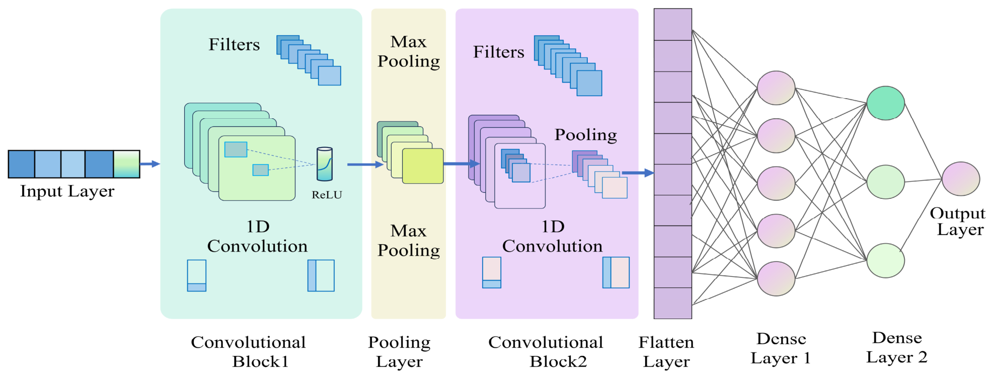
where R_i,j represents the pooling window. In single-variable electricity demand forecasting, 1D CNNs have been widely adopted [37,54]. A typical 1-dimensional CNN architecture is shown in Figure 1.

2.4. Attention Mechanism

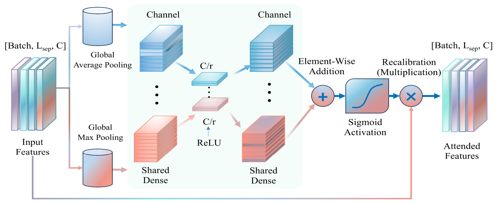
Attention mechanisms adaptively assign greater weight to informative elements and have been applied in many fields, including wearable-sensor activity recognition [55], battery state-of-health estimation [56], and heterogeneous vehicle trajectory prediction [57]. In load forecasting, Wang et al. [58] integrated time-domain features with wavelet-based frequency-domain features and used attention to emphasize abrupt changes and peak-demand periods. Wu et al. [59] combined EEMD with temporal and feature-level attention to improve nonstationary load forecasting and anomaly detection. Unlike these applications, which mainly apply attention to recurrent hidden states, fused time–frequency features, or multidimensional sensor signals, the present study applies channel attention to the concatenated outputs of five parallel convolutional branches. This design enables the model to adaptively reweight features associated with different temporal scales before the dense regression layers. Figure 2 illustrates the channel attention mechanism used in this study.

Suppose the input feature map is X ∈ R^H×W×C(2D) or X ∈ R^T×C (1D), where H and W are spatial dimensions, T is the time step, and C is the number of channels. First, spatial or temporal information is aggregated through global pooling operations to generate the following channel descriptors:

$$Z_{avg}={\displaystyle \frac{1}{\mathrm{S}}}{\displaystyle \sum _{i\in S}{X}_i}$$

(15)

$$Z_{\max }=\underset{i\in S}{\max }{X}_i$$

(16)

where S denotes the spatial domain (H × W) or the temporal domain (T). The pooled features are then processed using a shared multi-layer perceptron (MLP), and a bottleneck structure is introduced to reduce computational complexity.

$$f_{avg}=W_2\cdot \delta (W_1\cdot z_{avg})$$

(17)

$$f_{\max }=W_2\cdot \delta (W_1\cdot z_{\max })$$

(18)

where W₁ ∈ R^C×(c/r) and W₂ ∈ R^(c/r)×C are trainable weight matrices, r is the compression ratio, and δ(•) denotes the ReLU activation function. By combining the outputs from the average and max pooling paths and applying the Sigmoid function, the following channel attention map is generated:

$$\mathrm{S}=\sigma (f_{avg}+f_{\max })$$

(19)

where σ(•) represents the sigmoid function, S ∈ [0, 1], and C denotes the importance weights for each channel. Finally, the attention weights are fused via a channel-wise multiplication, as shown in the following equation:

$$\widehat{X}=X\otimes S$$

(20)

where ⊗ denotes channel-by-channel broadcast multiplication.

2.5. Hyperparameter Optimization

The performance of machine learning algorithms depends heavily on the choice of hyperparameters. Hyperband is an efficient algorithm designed specifically to tune the hyperparameters of machine learning models [60]. Unlike Bayesian optimization or grid search, which require predefined parameter ranges, Hyperband relies purely on random sampling and makes no assumptions about the smoothness of the hyperparameter space, making it more resilient. In scenarios with limited resources, Hyperband greatly enhances search efficiency and is especially useful for large hyperparameter spaces. Hyperband has gained widespread use in machine learning [61,62], and this paper employs it to fine-tune the model’s hyperparameters.

2.6. The Proposed Hybrid Forecasting Model

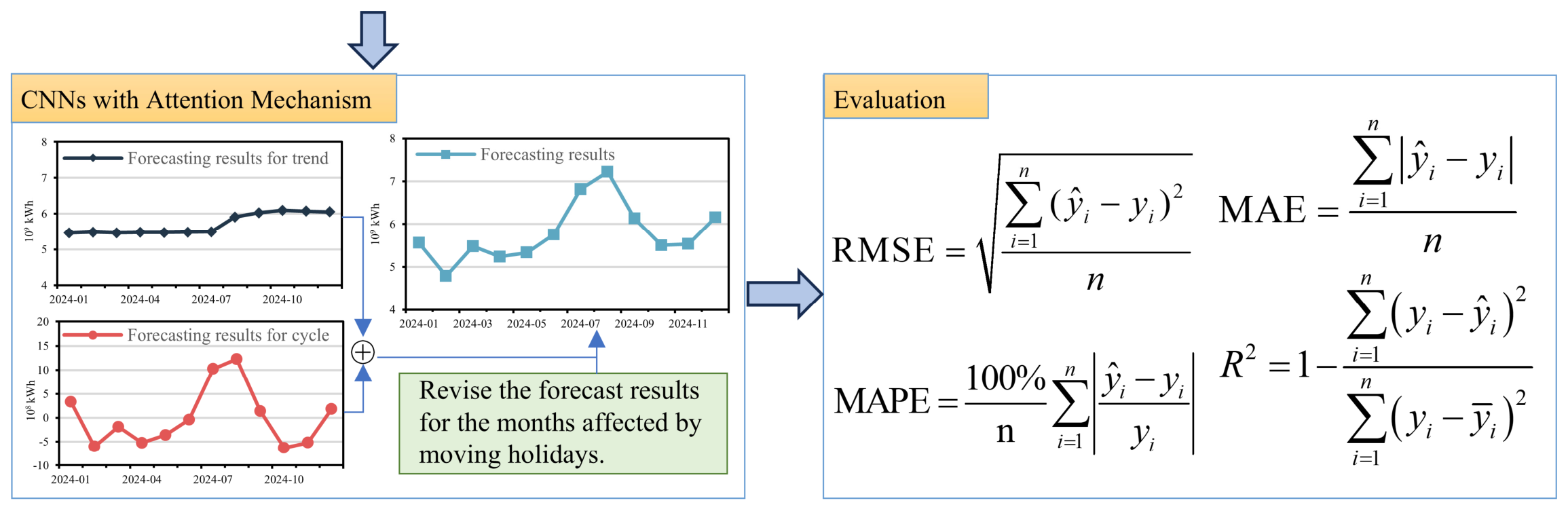
This paper proposes a new hybrid forecasting model for monthly electricity demand, abbreviated as X13-HP-CNN-ATT. The forecasting process of this model is as follows:

Step 1—Data preparation: Gather and arrange monthly electricity demand data, determine the type of moving-holiday effect, and compute the moving-holiday effect variable appropriate for regARIMA analysis.

Step 2—Data preprocessing: Use the regARIMA module in X13 to process the raw electricity demand data, detect outliers, estimate the impact of moving holidays, and apply suitable corrections to produce a time series with outliers and the moving-holiday effect removed.

Step 3—Time series decomposition: Use an HP filter on the time series, adjusted for outliers and holiday effects, to separate it into trend and cyclical components.

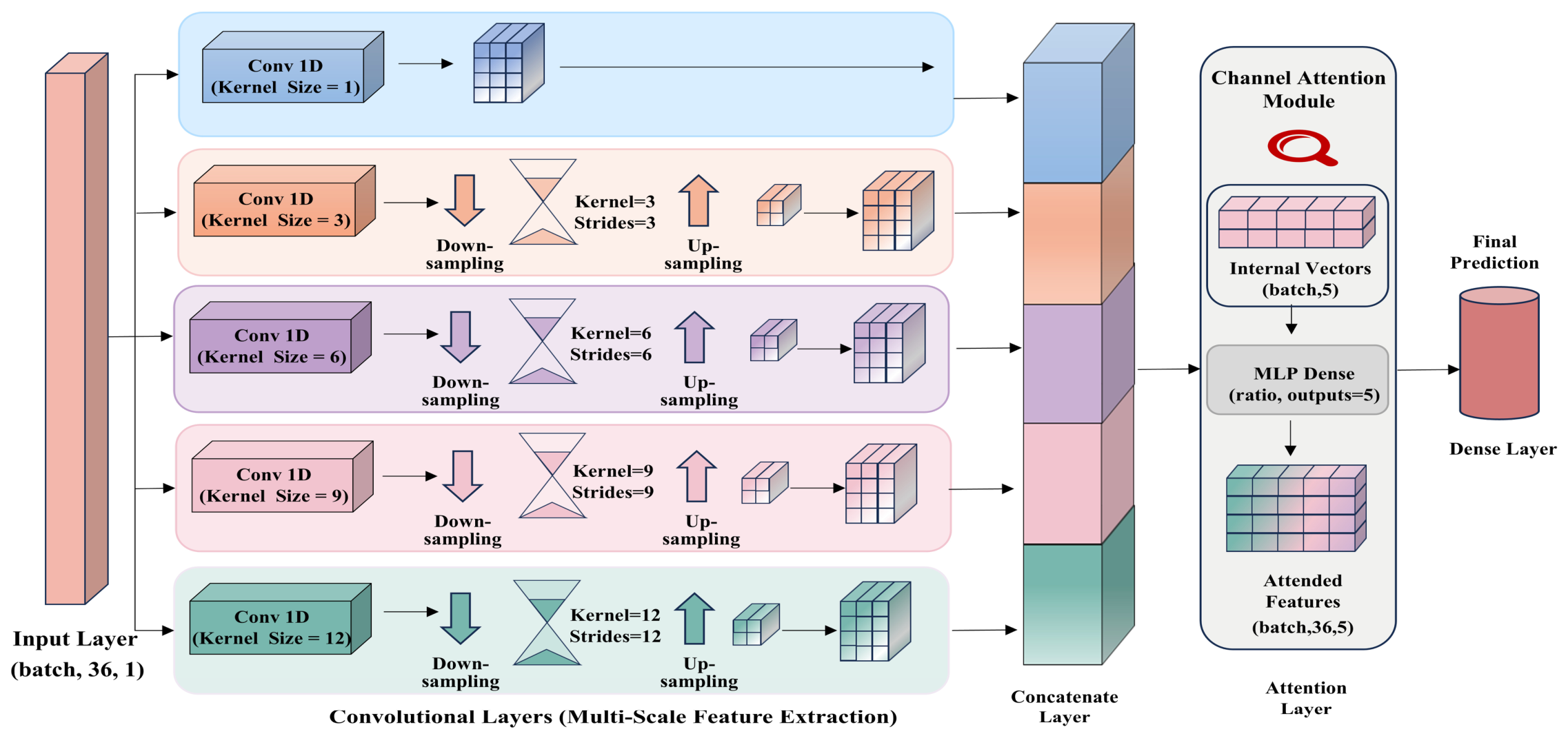
Step 4—Component sequence forecasting. To effectively capture the patterns of variation in electricity demand across different cycles (frequencies), this paper specifically designs a multi-branch parallel CNN incorporating an attention mechanism to forecast component sequences of electricity demand. Figure 3 shows a schematic diagram of the multi-branch CNN with an attention mechanism designed in this paper.

First, multi-branch CNNs extract various periodic components of electricity demand. An upsampling layer restores the extracted features to match the input data’s scale. The features are then combined through a concatenation layer. A channel attention mechanism helps the model focus on the most relevant feature channels for the current prediction task while filtering out irrelevant or redundant channels. The refined information passes through two dense layers. A dropout layer is included to prevent overfitting and improve generalization. Finally, a dense layer with a single output unit generates the prediction.

Table 1. Parameter settings of convolutional neural networks (CNNs).

No.	Convolutional Layer	Up Sampling
Branch 1	filters = 1, kernel size = 1, padding = same	/
Branch 2	filters = 1, kernel size = 3, padding = same, strides = 3	size = 3
Branch 3	filters = 1, kernel size = 6, padding = same, strides = 6	size = 6
Branch 4	filters = 1, kernel size = 9, padding = same, strides = 9	size = 9
Branch 5	filters = 1, kernel size = 12, padding = same, strides = 12	size = 12

lists the specific CNN parameter settings.

The kernel sizes 1, 3, 6, 9, and 12 were chosen to represent 1-, 3-, 6-, 9-, and 12-month periodicities in monthly demand. The channel-attention bottleneck was constrained to 1–4 units because the concatenated branches produce five feature channels.

In this paper, the neural network input sequence length is set to 36, meaning that electricity demand data from the first 36 months are used to predict the 37th month’s demand. A single convolutional kernel is employed in each CNN branch to extract features. Although each CNN branch uses only one convolutional kernel, we utilize kernels of different sizes to detect features with various periodic patterns. To enhance the model’s training and prediction abilities, this paper employs Hyperband to tune certain hyperparameters.

Table 2. Hyperparameter search space and key parameters.

Parameter Name	Parameter Search Space Range
Attention bottleneck units	min_value = 1, max_value = 4, step = 1
Units of dense layer 1	min_value = 32, max_value = 256, step = 12
Units of dense layer 2	min_value = 64, max_value = 128, step = 12
Dropout rate	min_value = 0.10, max_value = 0.50
Compile ()
Learning rate	min_value = 1 × 10−4, max_value = 1 × 10−2, step = 10, sampling = log
loss	Mean Squared Error
metrics	[mae, mape]
Trend component
Hyperband ()	objective = val_loss, max_epochs = 20, hyperband_iterations = 3
Early stopping ()	monitor = val_loss, patience = 8, mode = min
Search ()	epochs = 30, batch_size = 8, shuffle = False
Cycle component
Hyperband ()	objective = val_loss, max_epochs = 30, hyperband_iterations = 3
Early stopping ()	monitor = val_loss, patience = 8, mode = min
Search ()	epochs = 50, batch_size = 8, shuffle = False

displays the Hyperband hyperparameter search space and the main parameter settings.

Although the trend and cyclical components have different dynamics, both components were modeled with the same CNN-ATT architecture to keep component comparisons and baseline comparisons fair. Instead of using one fixed configuration, Hyperband searched each component separately: the trend component used max_epochs = 20 and search_epochs = 30, while the cyclical component used max_epochs = 30 and search_epochs = 50 (Table 2).

Step 5—Reconstruction and adjustment of forecast results: CNNs with attention mechanisms are used to predict the trend and seasonal components of electricity demand, producing forecasts for each component. Summing these individual forecast results provides the initial forecast. X13 was allowed to select a logarithmic transformation automatically. When that transformation was selected, the estimated holiday effects were applied multiplicatively to the reconstructed original-scale forecast; otherwise, they were added linearly. This correction was applied only to January and February, while the remaining months retained the preliminary component forecasts.

Step 6—Evaluation of prediction results: This paper assesses the model’s prediction accuracy using four commonly used prediction error metrics—RMSE, MAPE, MAE, and R²—as shown in Equations (21)–(24), and compares it with the baseline model’s performance to verify the effectiveness of the proposed prediction method.

$$\mathrm{RMSE}=\sqrt{{\displaystyle \frac{{\displaystyle \sum _{i=1}^n{({\widehat{y}}_i-y_i)}^2}}{n}}}$$

(21)

$$\mathrm{MAPE}={\displaystyle \frac{100\%}{\mathrm{n}}}{\displaystyle \sum _{i=1}^n\left|\frac{{\widehat{y}}_i-y_i}{y_i}\right|}$$

(22)

$$\mathrm{MAE}={\displaystyle \frac{{\displaystyle \sum _{i=1}^n\left|{\widehat{y}}_i-y_i\right|}}{n}}$$

(23)

$$R^2=1-{\displaystyle \frac{{\displaystyle \sum _{i=1}^n{\left(y_i-{\widehat{y}}_i\right)}^2}}{{\displaystyle \sum _{i=1}^n{\left(y_i-{\overline{y}}_i\right)}^2}}}$$

(24)

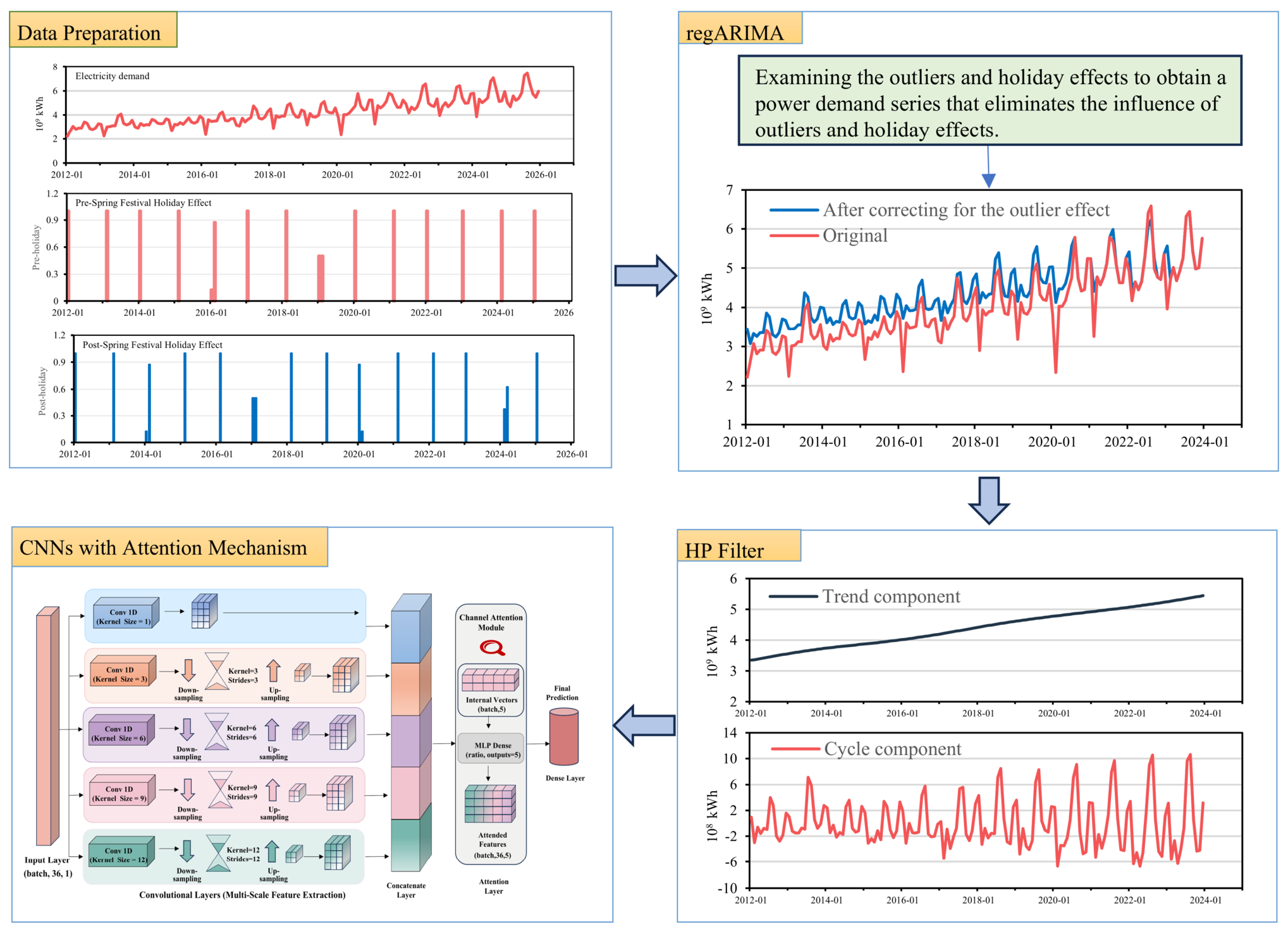
where ŷ_i and y_i represent the predicted and the actual observed values, ȳ_i denotes the mean of the observed values, and n is the number of data points. Figure 4 shows the prediction process of the proposed hybrid prediction model, X13-HP-CNN-ATT.

3. Results

3.1. Data

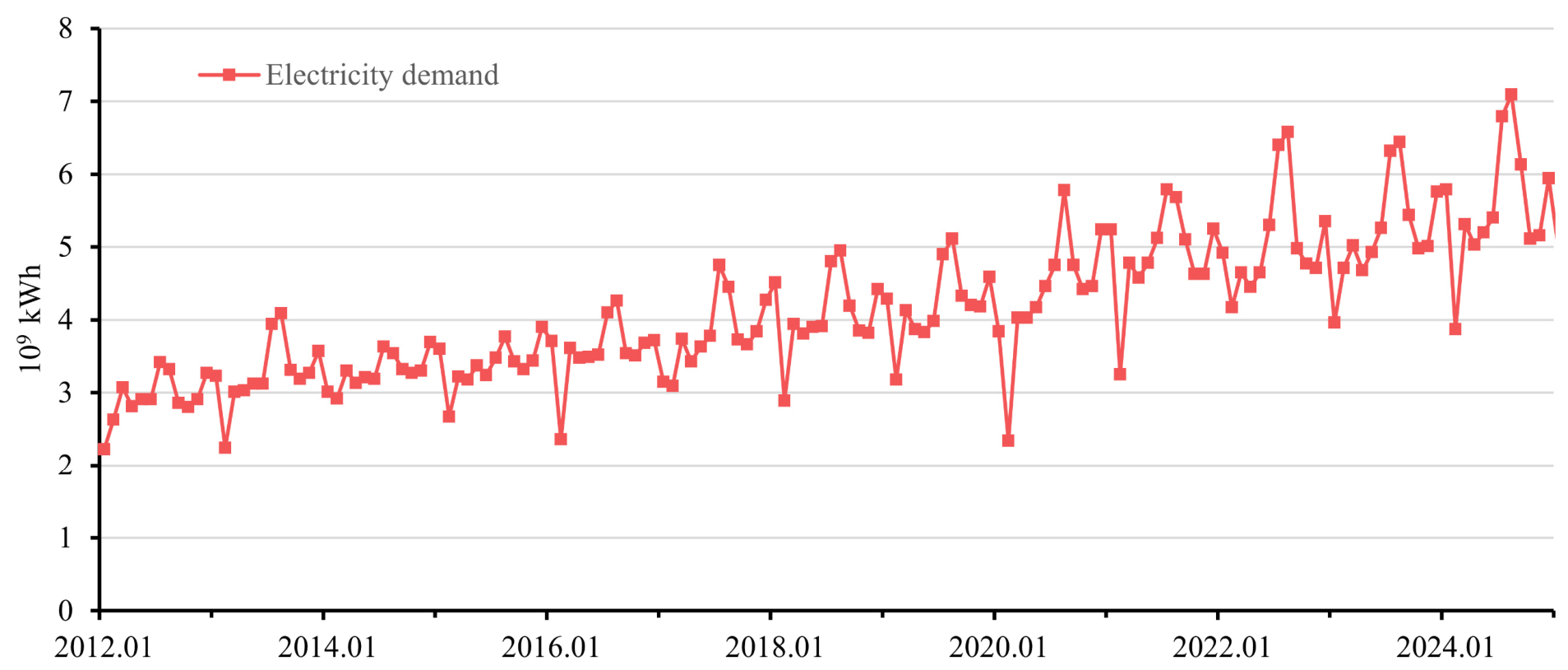
In this study, we compiled the monthly total electricity consumption dataset of Changzhou, Jiangsu Province, China, spanning the period from 2012 to 2025. The original data source was officially obtained from the Changzhou Municipal Bureau of Statistics (https://tjjyw.changzhou.gov.cn/cztjj/mbWeb_CZ.actio, accessed on 10 March 2026). In addition, monthly electricity demand data from Guangzhou (https://tjj.gz.gov.cn/datav/admin/home/www_report, accessed on 12 September 2026), spanning the period from 2012 to 2025, were compiled for the same period and used only for a cross-city robustness check.

As illustrated in Figure 5, Changzhou’s electricity demand exhibited a generally upward trend from 2012 to 2025. Fluctuations were more pronounced in some years. The annual low point usually occurs in February, while the peak occurs in July and August. Owing to pandemic control measures, the declines in February 2020 and 2021 were substantially larger than in other years.

Since the Spring Festival holiday shifts each year, demand patterns in January and February also vary, and the demand growth rate has changed since 2020. The forecasting model presented here specifically accounts for these issues by considering outliers and the effects of moving holidays, thereby enhancing forecast accuracy.

To assess the impact of the Spring Festival moving holiday, this paper relies on the authors’ previous findings. The effect variable is defined in two segments covering eight days before and eight days after the festival, and the two effects are allowed to differ. For each target year, model construction and evaluation followed a strictly causal rolling one-step protocol.

For the 2024 evaluation, regARIMA estimation, HP decomposition, sequence construction, standardization, training, and Hyperband validation used observations from January 2012 to December 2023. Within this training window, the final 20% of the chronologically ordered samples served as the validation set for hyperparameter selection and early stopping. The selected model was then held fixed while 12 one-step forecasts for 2024 were generated. For each forecast month, X13 adjustment and HP decomposition were updated only with observations strictly before the target month, so neither the target observation nor any future observation entered the input, scaler, regARIMA, HP, or neural network stage; these updates did not alter the already selected model or hyperparameters. The same procedure was repeated for 2025 after model construction on observations up to December 2024. A fixed random seed (42) and three Hyperband iterations were used for all models. The same automatic X13 log-selection option was used for every X13-based model. The Guangzhou cross-city evaluation followed the same causal rolling one-step protocol, X13-HP decomposition, chronological train/validation split, random seed 42, and three-iteration Hyperband budget used for Changzhou.

3.2. Correction for Outliers and Holiday Effects

Table 3. Estimation results for outliers and moving-holiday effect variables.

Samples	Outliers	Estimate	t Value	Holiday Effect	Estimate	t Value
2 January 2012–December 2023	AO 2020. Feb	−13.15	−7.63	Pre−holiday	−4.99	−6.86
	LS 2020. Aug	0.83	5.30	Post−holiday	−2.89	−2.85
	AO 2023. Jan	−8.21	−4.10	/	/	/
January 2012–December 2023	AO 2020. Feb	−13.31	−8.01	Pre−holiday	−5.15	−8.05
	AO 2020. Jul	−7.60	−5.26	Post−holiday	−2.93	−3.08
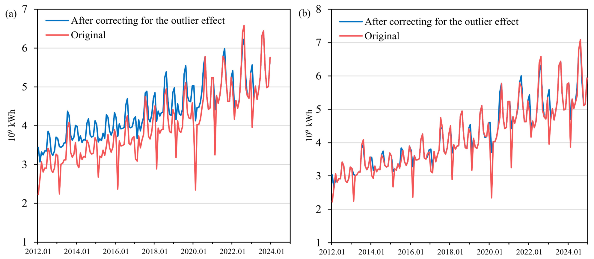
	AO 2023. Jan	−8.19	−4.53	/	/	/

lists the outliers detected by regARIMA and the estimates for the moving-holiday effect variables. After preprocessing the raw electricity demand data using regARIMA, over the period from January 2012 to December 2023, the program automatically identified three outliers at the 5% level. Two of these were additive outliers, occurring in February 2020 and January 2023, while one level-shift outlier occurred in August 2020 with a positive coefficient, indicating that electricity demand rose to a new level from that month onward. The statistical results for the holiday effect variables, before and after the Spring Festival, are significant and negative, and the estimated values differ, indicating that the prior specification of the moving-holiday effect variable is correct and valid. Despite our adjustment for the Spring Festival holiday effect, the statistical results also show that February 2020 and January 2023 remain outliers, suggesting that the COVID-19 pandemic has indeed altered electricity demand patterns.

Statistical results covering the period from January 2012 to December 2024 show similar patterns, except that the August 2020 data are no longer identified as an outlier; instead, the July 2020 data are now recognized as an additive outlier. The estimates and significance levels for the other variables remain largely unchanged. This change indicates that the additional post-pandemic observations help regARIMA distinguish a permanent level shift from a temporary additive shock. When 2024 data are included, the abrupt July 2020 movement is better explained by an additive outlier, while the August 2020 movement is no longer estimated as a lasting level change.

Figure 6 compares the electricity demand series adjusted for outlier effects and the Spring Festival moving-holiday effect with the original series. The results of the electricity demand adjustment differ somewhat depending on the outlier-detection method. The Spring Festival holiday effect was partially corrected in both periods. The seasonal patterns in the preprocessed electricity demand series are clearer, and the amplitude of fluctuations has decreased significantly, creating better conditions for developing forecasting models.

3.3. Results of Sequence Decomposition

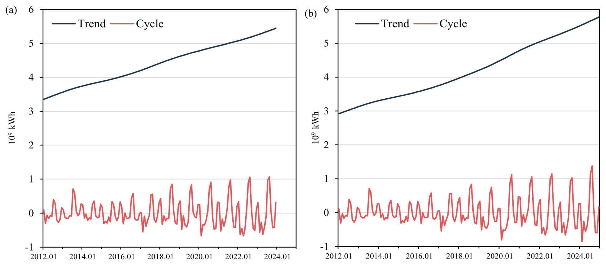
Applying an HP filter adjusted for outliers and holiday effects to electricity demand data allows us to further break down the data into a trend component that reflects long-term growth and a cyclical component that captures short-term seasonal variations. As illustrated in Figure 7, the trend component and seasonal patterns become more distinct after HP filtering, which enables the neural network model to better identify these patterns and improve its predictive accuracy. Figure 7a corresponds to the decomposition window ending in December 2023, which is used to construct the model for the 2024 forecasts; Figure 7b ends in December 2024 and is used for the 2025 forecasts. Comparing the two panels clarifies how much the trend and cyclical structures change when the training window is extended by one year.

3.4. Results of the Components Prediction

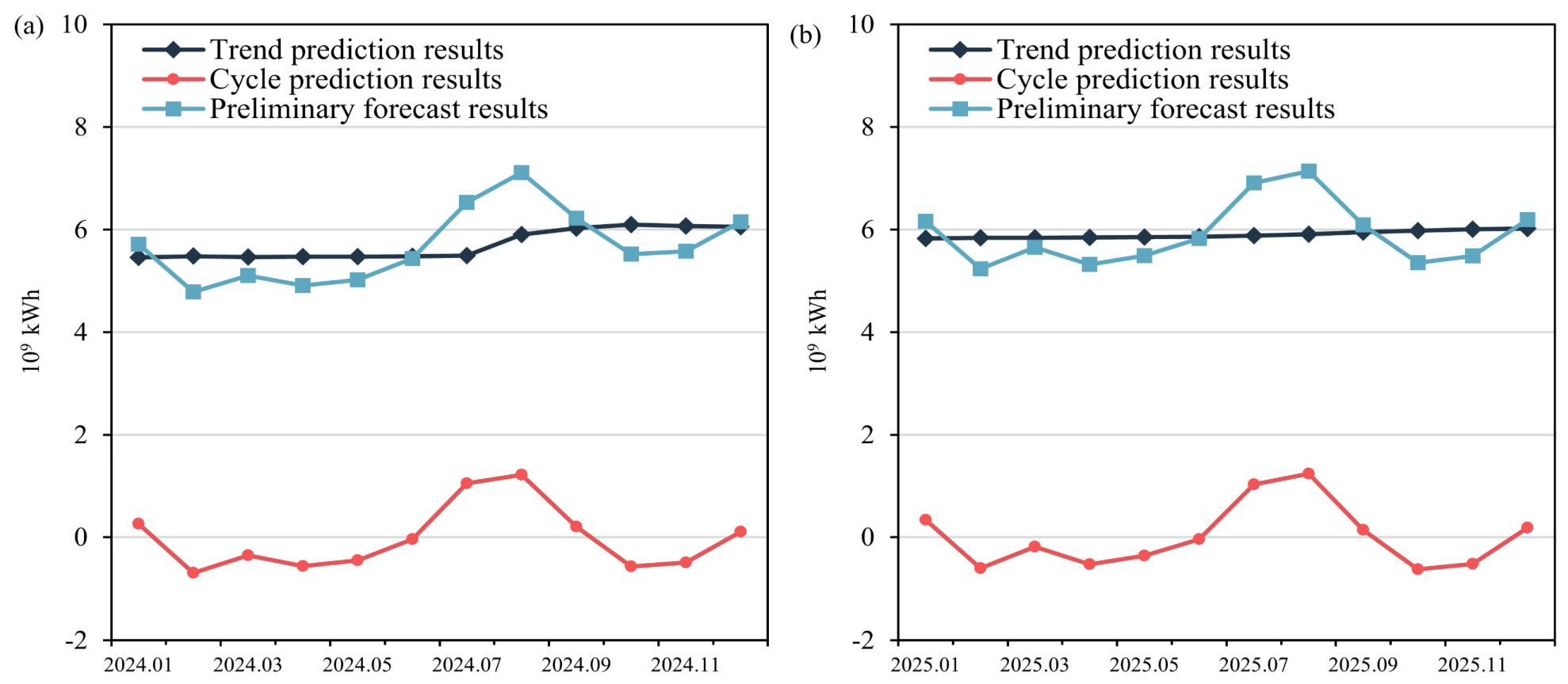
By employing CNNs with an attention mechanism to independently forecast the trend and cyclical components and then combining the results, we derive preliminary forecasts. Figure 8 shows the forecasting results for each component. It is evident that after July 2024, the growth trend in electricity demand levels off, and in 2025, it remains relatively steady. The forecast results for the cyclical component effectively reflect the seasonal patterns.

3.5. Comparison of Prediction Results

After generating preliminary forecast results, we refine the forecasts for January and February by adding the estimated values of the moving-holiday effect variable, through which we derive the final forecast outputs for these two months. To systematically validate the performance of our proposed method, we establish a set of benchmark models with distinct modeling strategies and conduct comparative analysis between their prediction results and those generated by X13-HP-CNN-ATT. All models used the same causal rolling one-step protocol, chronological 80/20 validation split, standardization, random seed (42), and three Hyperband iterations; only the architecture-specific modules and their search spaces differed.

3.5.1. Analysis of the Effect of Outlier or Moving-Holiday Correction and Series Decomposition

Initially, we built several forecasting models without adjusting for outliers or holiday effects and without applying an HP filter for time series decomposition, and then compared their forecasts with the method proposed in this paper. The construction methods for each model are as follows.

CNN-ATT: The data were used directly, without adjusting for outliers or moving-holiday effects and without series decomposition. CNNs with attention mechanisms are used to model and predict the raw electricity demand time series.

X13-CNN-ATT: regARIMA preprocesses the raw electricity demand series. CNNs with attention mechanisms model and forecast the outlier- and holiday-adjusted series, without using HP filters for decomposition.

HP-CNN-ATT: The HP filter is applied directly, without correcting for outliers or removing holiday effects, to decompose raw electricity demand into trend and cycle components, which are then forecast using CNNs with attention mechanisms.

Table 4. Evaluation metrics for predictive models that do not account for outliers, moving-holiday effects, or time series decomposition.

Model	2024				2025				Average
	RMSE	MAPE	MAE	R2	RMSE	MAPE	MAE	R2	RMSE	MAPE	MAE	R2
X13-HP-CNN-ATT	2.16	3.15	1.72	0.93	2.71	3.58	2.06	0.89	2.44	3.36	1.89	0.91
CNN-ATT	5.85	9.78	5.45	0.49	4.12	6.46	3.62	0.75	4.99	8.12	4.53	0.62
X13-CNN-ATT	2.70	4.47	2.36	0.89	3.12	4.17	2.52	0.86	2.91	4.32	2.44	0.87
HP-CNN-ATT	2.75	4.42	2.34	0.89	3.82	5.37	2.95	0.78	3.29	4.89	2.65	0.84

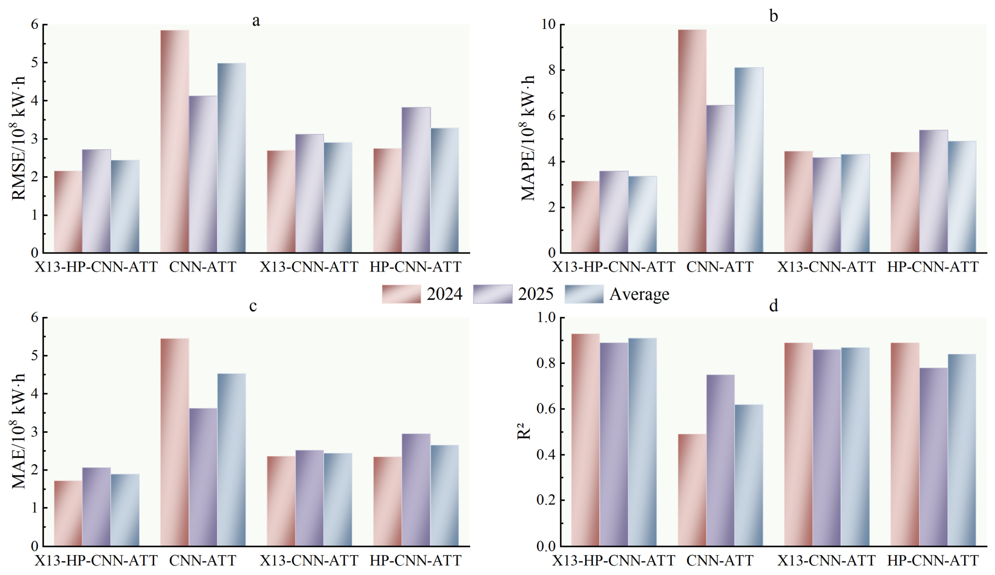
Notes: RMSE and MAE are in 10⁸ kWh; MAPE is a percentage; R² is unitless. Values were obtained under a unified rolling one-step protocol for 2024 and 2025.

and Figure 9 summarize the comparison of the basic architectures. Under the unified rolling one-step protocol, X13-CNN-ATT reduced the two-year average RMSE from 4.99 for CNN-ATT to 2.91, and X13-HP-CNN-ATT further reduced it to 2.44. The corresponding average MAPE values were 8.12%, 4.32%, and 3.36%, respectively. This pattern indicates that regARIMA preprocessing, especially the combination with HP decomposition, improved forecast accuracy.

HP-CNN-ATT produced a two-year average RMSE of 3.29 and R² of 0.84. Although HP decomposition reduced errors relative to the raw CNN baseline, the model remained less accurate than X13-HP-CNN-ATT, suggesting that outlier and moving-holiday corrections are needed before decomposition.

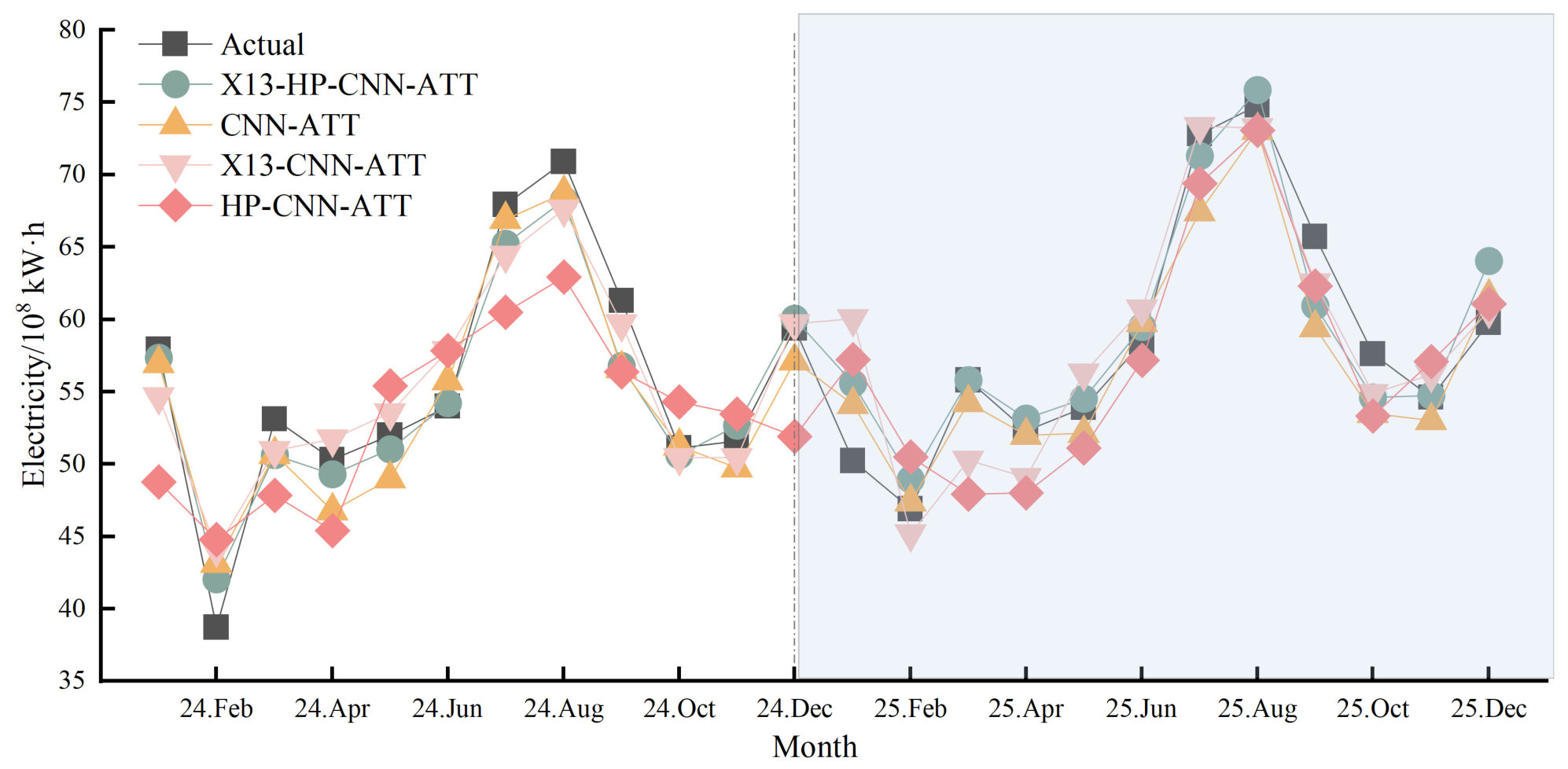
Figure 10 compares the actual and predicted monthly demand for X13-HP-CNN-ATT, X13-CNN-ATT, HP-CNN-ATT, and CNN-ATT. The proposed model tracked the seasonal pattern more closely in most months, especially during January–February and the summer peak.

Overall, X13-HP-CNN-ATT produced the lowest average RMSE and the most balanced performance across 2024 and 2025 among the basic architectures. These point estimates support the benefit of combining X13 adjustment with HP decomposition.

3.5.2. Comparison of Forecasting Performance Across Various CNN Architectures

To assess the effectiveness of the X13-HP-CNN-ATT network architecture, several CNNs with different branch structures were created, and their predictions were compared with those of X13-HP-CNN-ATT. A detailed description of the structure of each model is as follows.

X13-HP-CNN-B-ATT: Compared with X13-HP-CNN-ATT, the convolutional neural network branches with kernel sizes of 9 and 12 have been removed.

X13-HP-CNN-C-ATT: Compared with X13-HP-CNN-ATT, the convolutional neural network branch with a kernel size of 12 has been removed.

X13-HP-CNN-D-ATT: Compared with X13-HP-CNN-ATT, the convolutional neural network branch with a kernel size of 9 has been removed.

X13-HP-CNN-E-ATT: Compared with X13-HP-CNN-ATT, the convolutional neural network branch with a kernel size of 1 has been removed.

Table 5. Evaluation metrics for convolutional neural network prediction models using different network architectures.

Model	2024				2025				Average
	RMSE	MAPE	MAE	R2	RMSE	MAPE	MAE	R2	RMSE	MAPE	MAE	R2
X13-HP-CNN-ATT	2.16	3.15	1.72	0.93	2.71	3.58	2.06	0.89	2.44	3.36	1.89	0.91
X13-HP-CNN-B-ATT	2.68	3.97	2.22	0.89	2.55	3.60	2.08	0.90	2.61	3.78	2.15	0.90
X13-HP-CNN-C-ATT	1.97	3.19	1.78	0.94	2.95	3.72	2.15	0.87	2.46	3.46	1.97	0.91
X13-HP-CNN-D-ATT	2.37	3.80	2.13	0.92	2.89	3.68	2.17	0.88	2.63	3.74	2.15	0.90
X13-HP-CNN-E-ATT	2.48	3.89	2.15	0.91	3.09	3.99	2.43	0.86	2.79	3.94	2.29	0.88

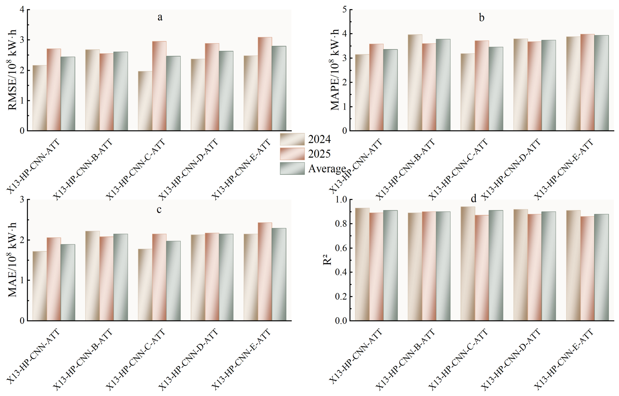
Notes: Branch labels follow Table 1. Metric units and the evaluation protocol are the same as in Table 4.

and Figure 11 present the branch-ablation results. The full model achieved the lowest two-year average RMSE (2.44), while X13-HP-CNN-C-ATT, the best reduced-branch model, achieved 2.46. X13-HP-CNN-B-ATT, X13-HP-CNN-D-ATT, and X13-HP-CNN-E-ATT followed with 2.61, 2.63, and 2.79. The differences between the full model and the branch variants were small and not statistically significant.

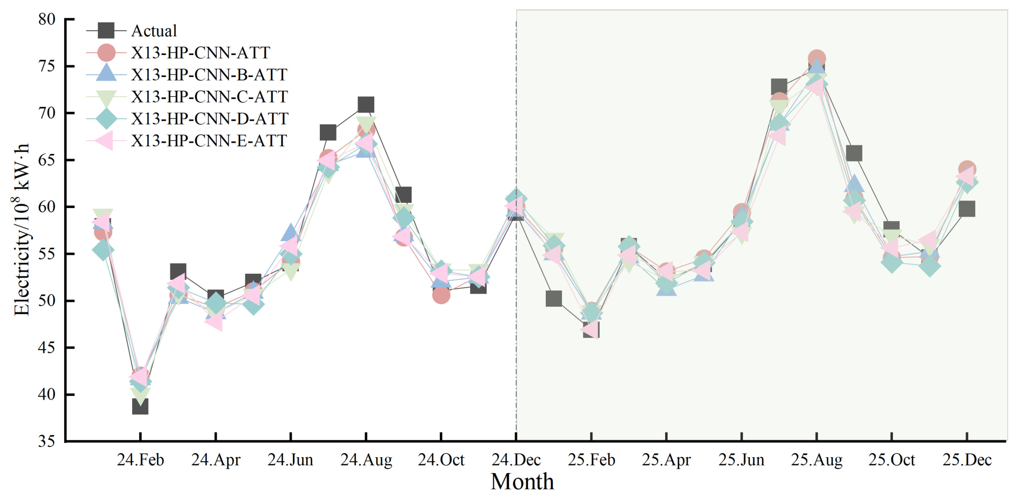
Figure 12 compares the monthly series of the full and branch-ablation models. The full model had the best two-year average metrics, but it was not significantly better than X13-HP-CNN-C-ATT. The branch variants tracked the observed seasonal pattern reasonably well. Their relative performance varied across years, indicating that branch importance is not stable enough to justify a strong architectural claim based on one test year.

3.5.3. Performance Comparison with Recurrent Neural Network Models

RNNs are widely used in time series modeling. To evaluate whether recurrent sequence modeling improves the proposed framework, we constructed several recurrent baselines and compared their forecasting accuracy with that of X13-HP-CNN-ATT. All baselines shared the same X13 adjustment, HP decomposition, input length, normalization, chronological validation split, random seed, early stopping rule, and three Hyperband iterations. The dense-layer, dropout, and learning-rate search spaces were identical to those in Table 2, whereas the recurrent unit counts were searched from 24 to 256 in steps of 24.

X13-HP-BiLSTM-ATT: This model replaces the multi-branch CNN in X13-HP-CNN-ATT with two Bi-LSTM layers followed by self-attention. All other components remain identical.

X13-HP-LSTM-ATT: This model replaces the multi-branch CNN in X13-HP-CNN-ATT with two LSTM layers followed by self-attention. All other components remain identical.

X13-HP-RNN-ATT: This model replaces the multi-branch CNN in X13-HP-CNN-ATT with two RNN layers followed by self-attention. All other components remain identical.

X13-HP-CNN-BiLSTM: This model retains the complete X13-HP-CNN-ATT framework and adds two Bi-LSTM layers with self-attention after the CNN feature-extraction stage. The recurrent units use the same search space and settings as X13-HP-BiLSTM-ATT.

Table 6. Evaluation metrics for several recurrent neural network prediction models.

Model	2024				2025				Average
	RMSE	MAPE	MAE	R2	RMSE	MAPE	MAE	R2	RMSE	MAPE	MAE	R2
X13-HP-CNN-ATT	2.16	3.15	1.72	0.93	2.71	3.58	2.06	0.89	2.44	3.36	1.89	0.91
X13-HP-BiLSTM-ATT	3.91	5.63	3.15	0.77	3.57	5.03	2.93	0.81	3.74	5.33	3.04	0.79
X13-HP-LSTM-ATT	3.41	4.14	2.45	0.83	4.24	5.94	3.61	0.73	3.82	5.04	3.03	0.78
X13-HP-RNN-ATT	3.50	4.05	2.35	0.82	3.75	5.35	3.19	0.79	3.63	4.70	2.77	0.80
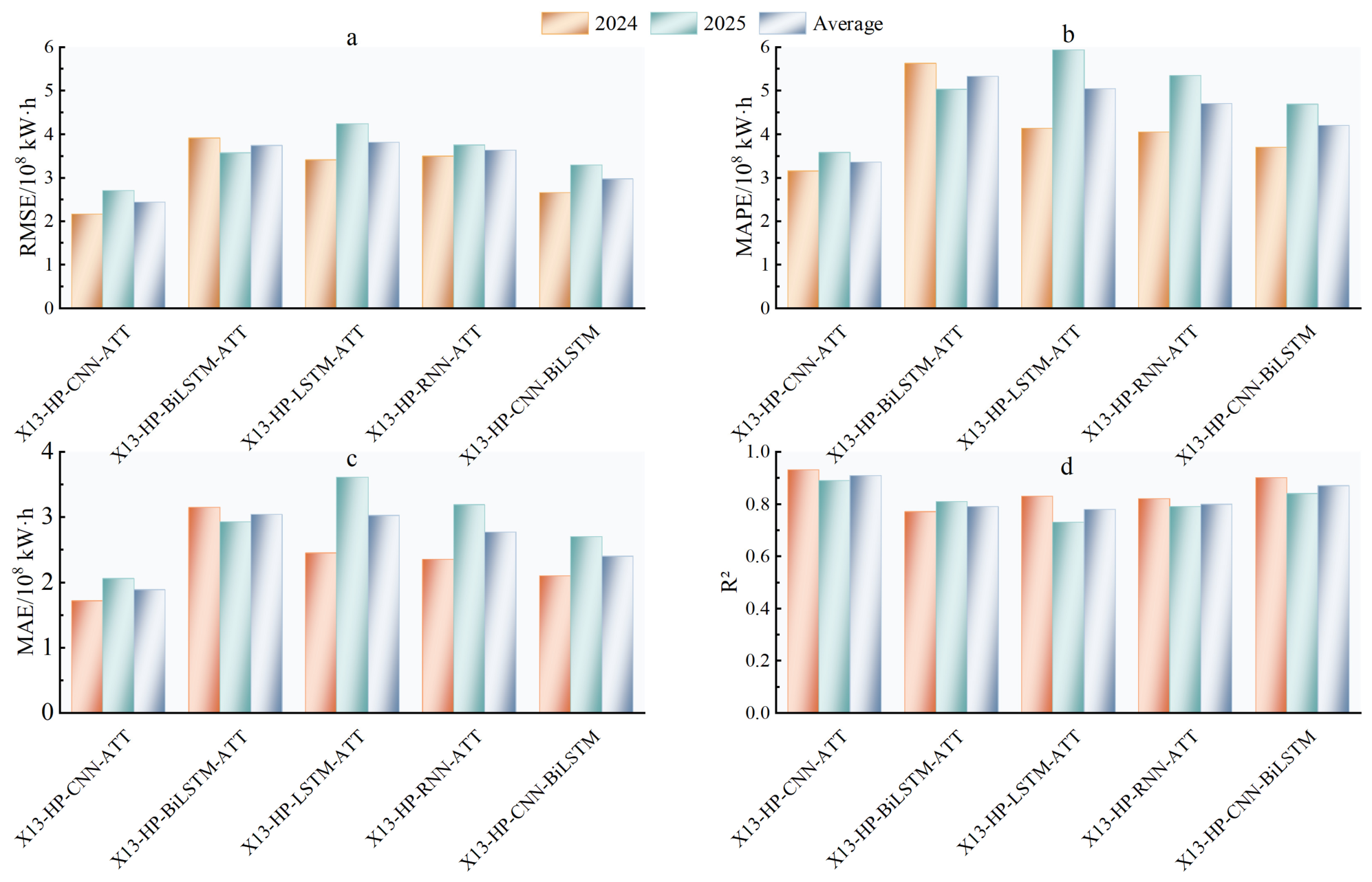
X13-HP-CNN-BiLSTM	2.65	3.70	2.10	0.90	3.29	4.69	2.70	0.84	2.97	4.20	2.40	0.87

compares X13-HP-CNN-ATT with four recurrent baselines under the same X13-HP decomposition and tuning protocol, and Figure 13 illustrates the mean values of these metrics for each model in 2024 and 2025. Metric units and the evaluation protocol are the same as in Table 4. The final selected Hyperband configurations for all compared models and components are provided in Supplementary Table S1.

X13-HP-CNN-ATT achieved the best RMSE, MAPE, MAE, and R² values in both years. The best-performing recurrent hybrid baseline was X13-HP-CNN-BiLSTM, which obtained average RMSE, MAPE, MAE, and R² values of 2.97, 4.20%, 2.40, and 0.87. Relative to this model, X13-HP-CNN-ATT reduced RMSE, MAPE, and MAE by approximately 17.80%, 20.00%, and 21.30%, respectively. The other recurrent baselines showed higher average errors and less consistent rankings across the two years. These results indicate that recurrent layers did not consistently improve forecasting accuracy under the unified evaluation protocol.

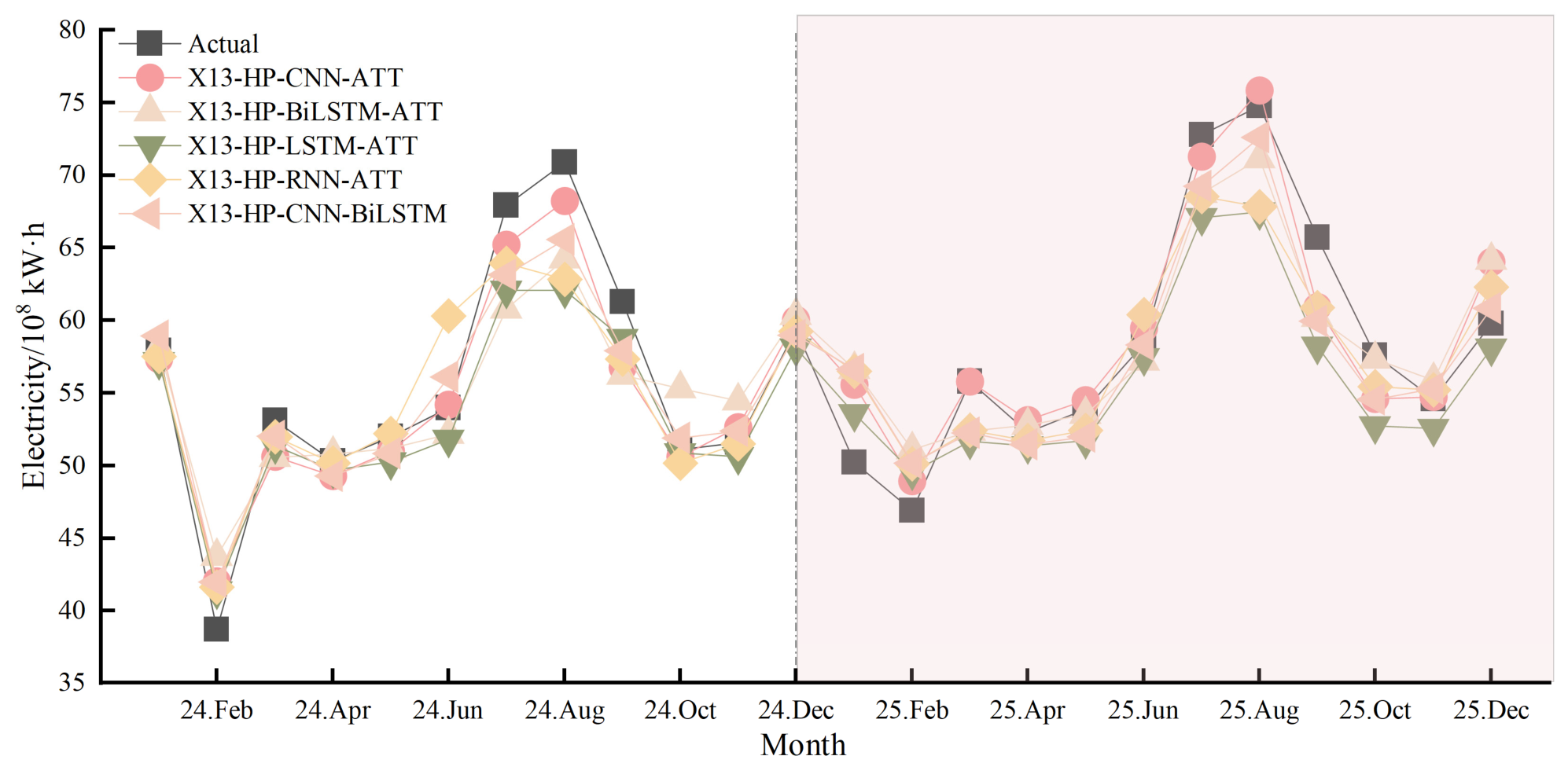
Figure 14 compares the actual and predicted series for the recurrent and hybrid baselines. The recurrent models captured the broad seasonal shape but showed larger deviations in some winter and summer months. These deviations were not uniform across years.

3.5.4. Statistical Significance Testing

To complement the annual point estimates in Table 4, Table 5 and Table 6, pairwise statistical tests were performed using the 24 monthly forecast errors from 2024 and 2025. For RMSE, the Diebold–Mariano (DM) statistic was computed from squared-error losses; for MAE, it was computed from absolute-error losses. The DM variance was estimated using a Newey–West HAC adjustment with two lags. Paired bootstrap resampling was performed over the monthly errors with 10,000 replications, and two-sided p-values and 95% confidence intervals were obtained for each error difference. Table 4, Table 5 and Table 6 report arithmetic means of the annual metrics, whereas

Table 7. Statistical comparisons between X13-HP-CNN-ATT and all comparison models.

Model	RMSE				MAE
	Diff	DM p	Boot. p	95% CI	Diff	DM p	Boot. p	95% CI
CNN-ATT	+2.61	0.0000	<0.0001	[1.54, 3.73]	+2.64	<0.0001	<0.0001	[1.61, 3.71]
X13-CNN-ATT	+0.47	0.1846	0.1361	[−0.15, 1.08]	+0.55	0.0613	0.0601	[−0.03, 1.11]
HP-CNN-ATT	+0.88	0.1549	0.0766	[−0.15, 1.79]	+0.76	0.0946	0.0676	[−0.04, 1.58]
X13-HP-CNN-B-ATT	+0.16	0.5152	0.5050	[−0.26, 0.67]	+0.26	0.2317	0.2141	[−0.12, 0.69]
X13-HP-CNN-C-ATT	+0.06	0.8167	0.8461	[−0.57, 0.55]	+0.08	0.6802	0.7585	[−0.43, 0.54]
X13-HP-CNN-D-ATT	+0.19	0.2819	0.3937	[−0.26, 0.63]	+0.26	0.1399	0.2327	[−0.17, 0.68]
X13-HP-CNN-E-ATT	+0.35	0.2288	0.1761	[−0.12, 0.89]	+0.40	0.1078	0.1014	[−0.07, 0.88]
X13-HP-BiLSTM-ATT	+1.29	0.0045	0.0001	[0.67, 1.95]	+1.15	0.0022	0.0007	[0.48, 1.82]
X13-HP-LSTM-ATT	+1.39	0.0700	0.0153	[0.23, 2.49]	+1.14	0.0327	0.0151	[0.25, 2.09]
X13-HP-RNN-ATT	+1.18	0.0492	0.0176	[0.22, 2.18]	+0.88	0.0760	0.0473	[0.06, 1.80]
X13-HP-CNN-BiLSTM	+0.54	0.0942	0.0571	[−0.04, 1.06]	+0.51	0.1003	0.0742	[−0.06, 1.06]

Diff: Comparison model minus X13-HP-CNN-ATT; DM p and Boot. p denote the two-sided p-values from the Diebold–Mariano test and paired bootstrap test.

uses the pooled 24 monthly errors; small aggregation differences may therefore occur. All comparisons are specified relative to X13-HP-CNN-ATT and are reported as per-comparison tests without multiplicity adjustment. Holm-adjusted DM results for both datasets and block-bootstrap confidence intervals for the Guangzhou analysis are provided in Supplementary Table S2.

Table 7 shows that X13-HP-CNN-ATT had positive RMSE and MAE differences in every pairwise comparison. The comparison with the strongest recurrent hybrid, X13-HP-CNN-BiLSTM, showed marginal evidence in favor of X13-HP-CNN-ATT. The pooled differences were +0.54 for RMSE and +0.51 for MAE. The paired bootstrap p-values were 0.0571 and 0.0742, respectively, while the DM p-values were 0.0942 and 0.1003. Both 95% confidence intervals narrowly included zero. These results indicate a consistent but marginal advantage at the 0.10 level, not conventional significance at the 0.05 level. Table 6 further shows that X13-HP-CNN-ATT reduced the two-year average RMSE and MAE by 17.8% and 21.3% relative to X13-HP-CNN-BiLSTM while using a simpler architecture. The proposed model therefore offers a favorable accuracy–complexity trade-off, although superiority over X13-HP-CNN-BiLSTM was not statistically established at the 0.05 level. Holm-adjusted p-values remain above 0.05 for both metrics. Differences from CNN-ATT and X13-HP-BiLSTM-ATT were significant for both metrics in both tests. Differences from X13-HP-LSTM-ATT and X13-HP-RNN-ATT were significant in at least one test for both metrics. Differences from X13-CNN-ATT, HP-CNN-ATT, and the branch-ablation models were not significant at the 0.05 level and should be interpreted as numerical.

Table 8. Selected Hyperband configurations for the trend and cyclical components of X13-HP-CNN-ATT.

Year	Component	Attention Bottleneck Units	Dense Layer 1 Units	Dense Layer 2 Units	Dropout	Learning Rate
2024	Trend	3	116	64	0.20	1 × 10−4
2024	Cycle	4	188	88	0.37	1 × 10−4
2025	Trend	3	68	100	0.33	1 × 10−3
2025	Cycle	4	200	88	0.49	1 × 10−3

lists the selected Hyperband configurations for the proposed model. All configurations were selected by minimum validation loss on the chronological validation set before the corresponding forecast year, and the selected values were not adjusted after inspecting test period performance.

3.5.5. Cross-City Comparison and Model Design Appropriateness

To assess cross-city robustness, the complete Changzhou protocol was repeated using Guangzhou for 2024 and 2025. For each target year, the model was constructed only from observations before January of that year, and the rolling one-step forecasts were updated strictly causally. The X13 adjustment, HP decomposition, standardization, chronological validation split, random seed 42, and three-iteration Hyperband budget were held constant across cities and model families. Consequently, the comparison isolates the effect of city-specific demand dynamics and model architecture rather than differences in tuning effort.

Table 9. Cross-city evaluation of all models in Guangzhou under the same causal rolling one-step protocol.

Model	2024				2025				Average
	RMSE	MAPE	MAE	R2	RMSE	MAPE	MAE	R2	RMSE	MAPE	MAE	R2
X13-HP-CNN-ATT	3.91	3.55	3.47	0.96	5.02	3.87	4.10	0.95	4.47	3.71	3.79	0.96
CNN-ATT	7.84	6.06	6.23	0.86	6.92	6.10	6.24	0.90	7.38	6.08	6.24	0.88
X13-CNN-ATT	5.14	4.75	4.59	0.94	6.28	4.40	4.67	0.92	5.71	4.57	4.63	0.93
HP-CNN-ATT	6.35	4.91	4.68	0.91	6.50	4.67	5.03	0.91	6.42	4.79	4.86	0.91
X13-HP-CNN-B-ATT	4.75	4.23	4.19	0.95	5.66	3.96	4.46	0.93	5.20	4.09	4.32	0.94
X13-HP-CNN-C-ATT	5.44	4.20	4.07	0.93	6.07	4.66	5.10	0.92	5.76	4.43	4.58	0.93
X13-HP-CNN-D-ATT	5.46	5.04	5.05	0.93	5.25	3.82	3.94	0.94	5.36	4.43	4.49	0.94
X13-HP-CNN-E-ATT	5.09	4.43	4.33	0.94	5.77	4.57	4.83	0.93	5.43	4.50	4.58	0.94
X13-HP-BiLSTM-ATT	6.53	4.54	5.01	0.90	6.71	5.43	5.80	0.91	6.62	4.98	5.41	0.91
X13-HP-LSTM-ATT	4.53	3.48	3.68	0.95	7.07	4.77	5.14	0.90	5.80	4.13	4.41	0.93
X13-HP-RNN-ATT	5.10	4.25	4.35	0.94	5.94	4.43	4.67	0.93	5.52	4.34	4.51	0.93
X13-HP-CNN-BiLSTM	3.08	2.71	2.72	0.98	4.97	3.37	3.72	0.95	4.03	3.04	3.22	0.96

compares all 12 models under the Guangzhou cross-city protocol. Across the two evaluation years, X13-HP-CNN-BiLSTM and X13-HP-CNN-ATT formed a clear leading pair. X13-HP-CNN-BiLSTM achieved the lowest average RMSE, MAE, and MAPE (4.03, 3.22, and 3.04%) and the highest average R² (0.96). X13-HP-CNN-ATT ranked second on all four aggregate metrics, with average RMSE, MAE, MAPE, and R² values of 4.47, 3.79, 3.71%, and 0.96. Thus, its average RMSE and MAE were only 0.44 and 0.57 higher, respectively, and its average MAPE was 0.67 percentage points higher, while the average R2 was identical to two decimal places. The next-lowest average RMSE values were 5.20 for X13-HP-CNN-B-ATT and 5.36 for X13-HP-CNN-D-ATT, leaving a clear margin between the leading pair and the remaining models. This aggregate ranking was consistent across years: X13-HP-CNN-BiLSTM ranked first according to RMSE in 2024 and 2025, X13-HP-CNN-ATT ranked second, and the corresponding RMSE gap narrowed from 0.83 to 0.05. X13-HP-CNN-ATT therefore provides a consistently competitive alternative to X13-HP-CNN-BiLSTM, approaching near-parity in 2025 while avoiding the two additional Bi-LSTM layers used by that model.

Table 10. Statistical comparisons between X13-HP-CNN-ATT and all comparison models in Guangzhou.

Model	RMSE				MAE
	Diff	DM p	Boot. p	95% CI	Diff	DM p	Boot. p	95% CI
CNN-ATT	+2.89	0.0076	0.0022	[1.01, 4.85]	+2.45	0.0039	0.0049	[0.75, 4.20]
X13-CNN-ATT	+1.24	0.0697	0.0124	[0.19, 2.16]	+0.84	0.1590	0.0720	[−0.07, 1.76]
HP-CNN-ATT	+1.93	0.0119	0.0148	[0.23, 3.31]	+1.07	0.0630	0.1884	[−0.50, 2.66]
X13-HP-CNN-B-ATT	+0.72	0.1721	0.1371	[−0.26, 1.63]	+0.54	0.2396	0.2644	[−0.41, 1.48]
X13-HP-CNN-C-ATT	+1.26	0.0519	0.0164	[0.19, 2.22]	+0.80	0.1898	0.1676	[−0.29, 1.94]
X13-HP-CNN-D-ATT	+0.86	0.0256	0.0146	[0.16, 1.51]	+0.71	0.0844	0.0696	[−0.07, 1.46]
X13-HP-CNN-E-ATT	+0.94	0.1028	0.0462	[0.04, 1.90]	+0.79	0.2077	0.1473	[−0.27, 1.85]
X13-HP-BiLSTM-ATT	+2.12	0.0260	0.0200	[0.52, 4.05]	+1.62	0.0233	0.0443	[0.17, 3.33]
X13-HP-LSTM-ATT	+1.44	0.1021	0.1496	[−0.66, 3.22]	+0.62	0.3795	0.4415	[−0.96, 2.24]
X13-HP-RNN-ATT	+1.03	0.0458	0.0517	[−0.08, 2.02]	+0.72	0.1478	0.1659	[−0.30, 1.74]
X13-HP-CNN-BiLSTM	−0.37	0.4318	0.5196	[−1.41, 0.71]	−0.57	0.2314	0.2324	[−1.47, 0.42]

Diff: Comparison model minus X13-HP-CNN-ATT; DM p and Boot. p denote the two-sided p-values from the Diebold–Mariano test and paired bootstrap test.

reports the pooled pairwise DM and paired bootstrap comparisons for the Guangzhou cross-city results. Positive differences indicate higher pooled error in the comparison model and therefore favor X13-HP-CNN-ATT. The proposed model had positive RMSE and MAE differences relative to 10 of the 11 alternatives. The only exception was X13-HP-CNN-BiLSTM, for which the pooled differences were −0.37 for RMSE and −0.57 for MAE. Neither difference was significant (DM p = 0.43 and 0.23, respectively), and both 95% bootstrap confidence intervals included zero. Although X13-HP-CNN-BiLSTM was the strongest alternative in Table 9, Table 10 provides no evidence of a statistically significant difference from the proposed model. By contrast, comparisons with CNN-ATT and X13-HP-BiLSTM-ATT were significant for both metrics under both tests. For X13-CNN-ATT, HP-CNN-ATT, X13-HP-CNN-C-ATT, X13-HP-CNN-D-ATT, X13-HP-CNN-E-ATT, and X13-HP-RNN-ATT, the RMSE advantage was significant in at least one test, whereas the corresponding MAE differences were not significant. Differences from X13-HP-CNN-B-ATT and X13-HP-LSTM-ATT were not significant for either metric or test. Together with its second-ranked RMSE in both years (Table 9), this pattern supports multi-scale CNN feature extraction and channel attention as the robust core of the proposed model. It also indicates that recurrent layers add value only when integrated effectively, rather than through additional recurrence alone.

4. Discussion

Electricity demand forecasting models based on deep learning frameworks have become a major area of current research; however, previous studies have paid little attention to the impact of outliers on accuracy. To address this, this paper first uses regARIMA to identify and handle outliers in monthly power demand time series. The case study results indicate that using the regARIMA module not only eliminates the effects of outliers—such as temporary level shifts and trend reversals—but also effectively handles fluctuations in monthly electricity demand caused by moving holidays. Since the preprocessed time series removes the influence of outliers and corrects for the moving-holiday effect, it helps the subsequent convolutional neural network more accurately identify patterns in electricity demand changes.

In addition, co-optimization of time series decomposition and deep learning has become the primary paradigm for building hybrid forecasting models [39]. The results of this paper also indicate that the method of first decomposing the monthly electricity demand time series into long-term trend and seasonal components, and then using a convolutional neural network to forecast each of the decomposed time series separately, does indeed improve the model’s forecasting accuracy.

The cross-city results clarify the role of recurrent layers. On the Changzhou dataset, X13-HP-CNN-BiLSTM did not improve over X13-HP-CNN-ATT. On the Guangzhou dataset, X13-HP-CNN-BiLSTM was the best model, but X13-HP-BiLSTM-ATT was among the weakest in 2024 and 2025. This contrast indicates that recurrent depth alone is not sufficient: recurrent layers become useful only when they are combined with a suitable multi-scale CNN feature extractor. The proposed X13-HP-CNN-ATT ranked second by RMSE in both Guangzhou years, and its pooled 24-month differences from X13-HP-CNN-BiLSTM were not statistically significant for RMSE (DM p = 0.43) or MAE (DM p = 0.23). Thus, the proposed design offers a more parsimonious and stable architecture for monthly electricity demand forecasting, while CNN-BiLSTM should be regarded as a promising extension when additional recurrent complexity is acceptable. Future work should evaluate alternative fusion forms, such as residual or parallel combination and gated integration layers, before drawing general conclusions about CNN-recurrent hybrids.

Overall, this paper proposes a method for constructing a monthly electricity demand forecasting model by combining traditional statistical methods with deep learning. This method is primarily built on a univariate framework. Therefore, it offers a practical advantage when socioeconomic, demographic, and meteorological variables are unavailable, and the statistical analyses of moving holidays and outliers can provide decision support.

Although we have proposed a method for robust forecasting of monthly electricity demand, several issues remain for future work. First, although the model was evaluated using Changzhou as the primary case and Guangzhou as an additional cross-city check, the evidence still covers only two cities. Additional cities with different climate, holiday, and industrial structures are needed to establish broader regional generalizability. Additionally, although the authors used HP filtering based on previous research, a significant number of studies have employed alternative decomposition techniques [45,46,63], and it remains to be seen whether these techniques outperform HP filtering.

5. Conclusions

Special events, such as extreme weather and the COVID-19 pandemic, can create abrupt changes in monthly electricity demand. This paper introduces a hybrid method that applies X13 regARIMA preprocessing, HP decomposition, and an attention-enhanced CNN to trend and cyclical components. Under a unified rolling one-step protocol, the method produced the lowest average error over 2024 and 2025 among the tested models on the primary Changzhou dataset. The strongest recurrent baseline had higher mean errors, but the advantage over it was marginal and did not reach conventional significance at the 0.05 level. The Guangzhou cross-city check further showed no statistically significant difference from the best CNN-BiLSTM variant, whereas a BiLSTM-only variant deteriorated substantially. These findings support the proposed multi-scale CNN and channel-attention design as a robust core in the tested settings and indicate that recurrent depth was beneficial only when combined with the convolutional front end.

The proposed method provides a practical approach to monthly electricity demand forecasting when external explanatory variables are unavailable. It reduced errors in most post-pandemic months and remained competitive in the primary city and cross-city check. Future work should expand the evaluation to more cities and decomposition methods and should report repeated random-seed stability before stronger general claims are made.

References

1. Gao, T.; Niu, D.; Ji, Z.; Sun, L. Mid-term electricity demand forecasting using improved variational mode decomposition and extreme learning machine optimized by sparrow search algorithm. Energy 2022, 261, 125328. [Google Scholar] [CrossRef] [Scilit]
2. Du, P.; Ye, Y.; Wu, H.; Wang, J. Study on deterministic and interval forecasting of electricity load based on multi-objective whale optimization algorithm and transformer model. Expert Syst. Appl. 2025, 268, 126361. [Google Scholar] [CrossRef] [Scilit]
3. Su, Z.; Zhang, J.; Yang, Z.; Ma, L. A hybrid monthly electricity demand forecasting model combining an Hodrick-Prescott filter, recurrent neural networks, and autoregressive integrated moving average. Energy AI 2025, 22, 100600. [Google Scholar] [CrossRef] [Scilit]
4. Hussain, F.; Hasanuzzaman, M.; Rahim, N.A. Multivariate machine learning algorithms for energy demand forecasting and load behavior analysis. Energy Convers. Manag. X 2025, 26, 100903. [Google Scholar] [CrossRef] [Scilit]
5. Zhang, T.; Zhang, X.; Rubasinghe, O.; Liu, Y.; Chow, Y.H.; Iu, H.H.C.; Fernando, T. Long-Term Energy and Peak Power Demand Forecasting Based on Sequential-XGBoost. IEEE Trans. Power Syst. 2024, 39, 3088–3104. [Google Scholar] [CrossRef] [Scilit]
6. Xu, H.; Hu, F.; Liang, X.; Zhao, G.; Abugunmi, M. A framework for electricity load forecasting based on attention mechanism time series depthwise separable convolutional neural network. Energy 2024, 299, 131258. [Google Scholar] [CrossRef] [Scilit]
7. Zhou, B.; Wang, H.; Xie, Y.; Li, G.; Yang, D.; Hu, B. Regional short-term load forecasting method based on power load characteristics of different industries. Sustain. Energy Grids Netw. 2024, 38, 101336. [Google Scholar] [CrossRef] [Scilit]
8. Rawal, K.; Ahmad, A. Mining latent patterns with multi-scale decomposition for electricity demand and price forecasting using modified deep graph convolutional neural networks. Sustain. Energy Grids Netw. 2024, 39, 101436. [Google Scholar] [CrossRef] [Scilit]
9. Al-Musaylh, M.S.; Deo, R.C.; Adamowski, J.F.; Li, Y. Short-term electricity demand forecasting with MARS, SVR and ARIMA models using aggregated demand data in Queensland, Australia. Adv. Eng. Inform. 2018, 35, 1–16. [Google Scholar] [CrossRef] [Scilit]
10. Ferbar Tratar, L.; Strmčnik, E. The comparison of Holt–Winters method and Multiple regression method: A case study. Energy 2016, 109, 266–276. [Google Scholar] [CrossRef] [Scilit]
11. de Oliveira, E.M.; Cyrino Oliveira, F.L. Forecasting mid-long term electric energy consumption through bagging ARIMA and exponential smoothing methods. Energy 2018, 144, 776–788. [Google Scholar] [CrossRef] [Scilit]
12. Cancelo, J.R.; Espasa, A.; Grafe, R. Forecasting the electricity load from one day to one week ahead for the Spanish system operator. Int. J. Forecast. 2008, 24, 588–602. [Google Scholar] [CrossRef] [Scilit]
13. Vu, D.H.; Muttaqi, K.M.; Agalgaonkar, A.P. A variance inflation factor and backward elimination based robust regression model for forecasting monthly electricity demand using climatic variables. Appl. Energy 2015, 140, 385–394. [Google Scholar] [CrossRef] [Scilit]
14. Hong, J.-H.; Lee, G.-C. Monthly Load Forecasting in a Region Experiencing Demand Growth: A Case Study of Texas. Energies 2025, 18, 4135. [Google Scholar] [CrossRef] [Scilit]
15. Yaprakdal, F.; Varol Arısoy, M. A Multivariate Time Series Analysis of Electrical Load Forecasting Based on a Hybrid Feature Selection Approach and Explainable Deep Learning. Appl. Sci. 2023, 13, 12946. [Google Scholar] [CrossRef] [Scilit]
16. Zhang, T.; Zhang, X.; Iu, H.; Fernando, T. Long-term Monthly Energy and Peak Demand Forecasting Based on Sequential-XGBoost. In Proceedings of the 2023 IEEE 5th International Conference on Power, Intelligent Computing and Systems (ICPICS), Shenyang, China, 14–16 July 2023; pp. 157–162. [Google Scholar]
17. Zhang, Y.; Li, X.-X.; Xin, R.; Chew, L.W.; Liu, C.-H. Applicability of data-driven methods in modeling electricity demand-climate nexus: A tale of Singapore and Hong Kong. Energy 2024, 300, 131525. [Google Scholar] [CrossRef] [Scilit]
18. Herodotou, P.; Tziolis, G.; Makrides, G.; Georghiou, G.E. Comparative analysis of machine learning methods for residential net load forecasting of solar-integrated households. Sustain. Energy Grids Netw. 2026, 45, 102106. [Google Scholar] [CrossRef] [Scilit]
19. Cheng, S.; Shi, J.; Cheng, Q.; Zhou, X.; Zeng, S. Hybrid Model for Medium-Term Load Forecasting in Urban Power Grids. Energies 2025, 18, 4378. [Google Scholar] [CrossRef] [Scilit]
20. Mukherjee, S.; Nateghi, R. Climate sensitivity of end-use electricity consumption in the built environment: An application to the state of Florida, United States. Energy 2017, 128, 688–700. [Google Scholar] [CrossRef] [Scilit]
21. Rai, S.; De, M. Analysis of classical and machine learning based short-term and mid-term load forecasting for smart grid. Int. J. Sustain. Energy 2021, 40, 821–839. [Google Scholar] [CrossRef] [Scilit]
22. Chang, P.C.; Fan, C.Y.; Lin, J.J. Monthly electricity demand forecasting based on a weighted evolving fuzzy neural network approach. Int. J. Electr. Power Energy Syst. 2011, 33, 17–27. [Google Scholar] [CrossRef] [Scilit]
23. Oreshkin, B.N.; Dudek, G.; Pełka, P.; Turkina, E. N-BEATS neural network for mid-term electricity load forecasting. Appl. Energy 2021, 293, 116918. [Google Scholar] [CrossRef] [Scilit]
24. Chaturvedi, S.; Rajasekar, E.; Natarajan, S.; McCullen, N. A comparative assessment of SARIMA, LSTM RNN and Fb Prophet models to forecast total and peak monthly energy demand for India. Energy Policy 2022, 168, 113097. [Google Scholar] [CrossRef] [Scilit]
25. Moon, Y.; Lee, Y.; Hwang, Y.; Jeong, J. Long Short-Term Memory Autoencoder and Extreme Gradient Boosting-Based Factory Energy Management Framework for Power Consumption Forecasting. Energies 2024, 17, 3666. [Google Scholar] [CrossRef] [Scilit]
26. Hong, W.C. Electric load forecasting by seasonal recurrent SVR (support vector regression) with chaotic artificial bee colony algorithm. Energy 2011, 36, 5568–5578. [Google Scholar] [CrossRef] [Scilit]
27. Cao, G.; Wu, L. Support vector regression with fruit fly optimization algorithm for seasonal electricity consumption forecasting. Energy 2016, 115, 734–745. [Google Scholar] [CrossRef] [Scilit]
28. Askari, M.; Keynia, F. Mid-term electricity load forecasting by a new composite method based on optimal learning MLP algorithm. IET Gener. Transm. Distrib. 2020, 14, 845–852. [Google Scholar] [CrossRef] [Scilit]
29. Wu, F.; Cattani, C.; Song, W.; Zio, E. Fractional ARIMA with an improved cuckoo search optimization for the efficient Short-term power load forecasting. Alex. Eng. J. 2020, 59, 3111–3118. [Google Scholar] [CrossRef] [Scilit]
30. Jiang, W.; Wu, X.; Gong, Y.; Yu, W.; Zhong, X. Holt–Winters smoothing enhanced by fruit fly optimization algorithm to forecast monthly electricity consumption. Energy 2020, 193, 807–814. [Google Scholar] [CrossRef] [Scilit]
31. Hussein, A.; Awad, M. Time series forecasting of electricity consumption using hybrid model of recurrent neural networks and genetic algorithms. Meas. Energy 2024, 2, 100004. [Google Scholar] [CrossRef] [Scilit]
32. Wang, J.; Zhu, W.; Zhang, W.; Sun, D. A trend fixed on firstly and seasonal adjustment model combined with the ε-SVR for short-term forecasting of electricity demand. Energy Policy 2009, 37, 4901–4909. [Google Scholar] [CrossRef] [Scilit]
33. Wang, J.; Ma, X.; Wu, J.; Dong, Y. Optimization models based on GM (1,1) and seasonal fluctuation for electricity demand forecasting. Int. J. Electr. Power Energy Syst. 2012, 43, 109–117. [Google Scholar] [CrossRef] [Scilit]
34. Tang, T.; Jiang, W.; Zhang, H.; Nie, J.; Xiong, Z.; Wu, X.; Feng, W. GM(1,1) based improved seasonal index model for monthly electricity consumption forecasting. Energy 2022, 252, 124041. [Google Scholar] [CrossRef] [Scilit]
35. Yang, J.; Zhou, S.; Li, Y.; Wang, Y. Mid Term Power Load Forecasting Using Blending Integrated Model Based on Prophet, XGBoost, and LSTM. In Proceedings of the 2024 7th International Conference on Power and Energy Applications (ICPEA), Taiyuan, China, 18–20 October 2024; pp. 615–620. [Google Scholar]
36. Sharma, A.; Jain, S.K. A Novel Two-Stage Framework for Mid-Term Electric Load Forecasting. IEEE Trans. Ind. Inform. 2024, 20, 247–255. [Google Scholar] [CrossRef] [Scilit]
37. Shawon, S.M.; Haider, S.N.; Barua, A.; Austin, S.; Adan, I.A.; Hossain, M.S.; Zubair, H. Hybrid CNN-LSTM model for urban energy load forecasting with IGA-XAI for smart grids: Peak and off-peak variability insights. Results Eng. 2025, 28, 107245. [Google Scholar] [CrossRef] [Scilit]
38. Rubasinghe, O.; Zhang, X.; Chau, T.K.; Chow, Y.H.; Fernando, T.; Iu, H.H.-C. A Novel Sequence to Sequence Data Modelling Based CNN-LSTM Algorithm for Three Years Ahead Monthly Peak Load Forecasting. IEEE Trans. Power Syst. 2024, 39, 1932–1947. [Google Scholar] [CrossRef] [Scilit]
39. Shao, Z.; Chao, F.; Yang, S.-L.; Zhou, K.-L. A review of the decomposition methodology for extracting and identifying the fluctuation characteristics in electricity demand forecasting. Renew. Sustain. Energy Rev. 2017, 75, 123–136. [Google Scholar] [CrossRef] [Scilit]
40. González-Romera, E.; Jaramillo-Morán, M.A.; Carmona-Fernández, D. Monthly electric energy demand forecasting with neural networks and Fourier series. Energy Convers. Manag. 2008, 49, 3135–3142. [Google Scholar] [CrossRef] [Scilit]
41. Abu-Shikhah, N.; Elkarmi, F. Medium-term electric load forecasting using singular value decomposition. Energy 2011, 36, 4259–4271. [Google Scholar] [CrossRef] [Scilit]
42. Zhu, S.; Wang, J.; Zhao, W.; Wang, J. A seasonal hybrid procedure for electricity demand forecasting in China. Appl. Energy 2011, 88, 3807–3815. [Google Scholar] [CrossRef] [Scilit]
43. Bunnoon, P.; Chalermyanont, K.; Limsakul, C. Multi-substation control central load area forecasting by using HP-filter and double neural networks (HP-DNNs). Int. J. Electr. Power Energy Syst. 2013, 44, 561–570. [Google Scholar] [CrossRef] [Scilit]
44. Xiong, T.; Bao, Y.; Hu, Z. Interval forecasting of electricity demand: A novel bivariate EMD-based support vector regression modeling framework. Int. J. Electr. Power Energy Syst. 2014, 63, 353–362. [Google Scholar] [CrossRef] [Scilit]
45. Shao, Z.; Gao, F.; Yang, S.-L.; Yu, B.-G. A new semiparametric and EEMD based framework for mid-term electricity demand forecasting in China: Hidden characteristic extraction and probability density prediction. Renew. Sustain. Energy Rev. 2015, 52, 876–889. [Google Scholar] [CrossRef] [Scilit]
46. Niu, D.; Ji, Z.; Li, W.; Xu, X.; Liu, D. Research and application of a hybrid model for mid-term power demand forecasting based on secondary decomposition and interval optimization. Energy 2021, 234, 121145. [Google Scholar] [CrossRef] [Scilit]
47. Dudek, G.; Pelka, P.; Smyl, S. A Hybrid Residual Dilated LSTM and Exponential Smoothing Model for Midterm Electric Load Forecasting. IEEE Trans. Neural Netw. Learn Syst. 2022, 33, 2879–2891. [Google Scholar] [CrossRef] [Scilit] [PubMed]
48. Huang, Y.; Hasan, N.; Deng, C.; Bao, Y. Multivariate empirical mode decomposition based hybrid model for day-ahead peak load forecasting. Energy 2022, 239, 122245. [Google Scholar] [CrossRef] [Scilit]
49. Luzia, R.; Rubio, L.; Velasquez, C.E. Sensitivity analysis for forecasting Brazilian electricity demand using artificial neural networks and hybrid models based on Autoregressive Integrated Moving Average. Energy 2023, 274, 127365. [Google Scholar] [CrossRef] [Scilit]
50. Wang, L.; Wang, X.; Zhao, Z. Mid-term electricity demand forecasting using improved multi-mode reconstruction and particle swarm-enhanced support vector regression. Energy 2024, 304, 132021. [Google Scholar] [CrossRef] [Scilit]
51. Xu, Y.; Yu, Q.; Du, P.; Wang, J. A paradigm shift in solar energy forecasting: A novel two-phase model for monthly residential consumption. Energy 2024, 305, 132192. [Google Scholar] [CrossRef] [Scilit]
52. U.S. Census Bureau. X-13ARIMA-SEATS Reference Manual; Bureau USC: Washington, DC, USA, 2020.
53. Mehrhoff, J. Outlier Detection and Correction: Handbook on Seasonal Adjustment; Publications Office of the European Union: Luxembourg, 2018. [Google Scholar]
54. Buratto, W.G.; Muniz, R.N.; Nied, A.; Barros, C.; Finardi, E.C.; Gonzalez, G.V. Hybrid CF-CNN-BiLSTM hypertuned by Bayesian optimization for thermal power generation and decarbonization forecasting. Int. J. Electr. Power Energy Syst. 2025, 172, 111199. [Google Scholar] [CrossRef] [Scilit]
55. Khatun, M.A.; Yousuf, M.A.; Ahmed, S.; Uddin, M.Z.; Alyami, S.A.; Al-Ashhab, S.; Akhdar, H.F.; Khan, A.; Azad, A.; Moni, M.A. Deep CNN-LSTM With Self-Attention Model for Human Activity Recognition Using Wearable Sensor. IEEE J. Transl. Eng. Health Med. 2022, 10, 2700316. [Google Scholar] [CrossRef] [Scilit] [PubMed]
56. Tang, A.; Jiang, Y.; Yu, Q.; Zhang, Z. A hybrid neural network model with attention mechanism for state of health estimation of lithium-ion batteries. J. Energy Storage 2023, 68, 107734. [Google Scholar] [CrossRef] [Scilit]
57. Zhang, Q.; Xing, Y.; Wang, J.; Fang, Z.; Liu, Y.; Yin, G. Interaction-aware and driving style-aware trajectory prediction for heterogeneous vehicles in mixed traffic environment. IEEE Trans. Intell. Transp. Syst. 2025, 26, 10710–10724. [Google Scholar] [CrossRef] [Scilit]
58. Wang, J.; Wang, Y.; Ma, L.; Tian, L.; Zhang, Q. Electricity prediction based on time-frequency domain fusion and attention mechanism. Electr. Power Syst. Res. 2025, 249, 112094. [Google Scholar] [CrossRef] [Scilit]
59. Wu, Y.; Sun, W.; Li, Q. Power load forecasting and anomaly detection using a two-stage attention mechanism and deep neural networks. Electr. Power Syst. Res. 2025, 249, 112056. [Google Scholar] [CrossRef] [Scilit]
60. Li, L.; Jamieson, K.; DeSalvo, G.; Rostamizadeh, A.; Talwalkar, A. Hyperband: A novel bandit-based approach to hyperparameter optimization. J. Mach. Learn. Res. 2018, 18, 1–52. [Google Scholar]
61. Ling, Y.; Huang, T.; Yue, Q.; Shan, Q.; Hei, D.; Zhang, X.; Shi, C.; Jia, W. Improving the estimation accuracy of multi-nuclide source term estimation method for severe nuclear accidents using temporal convolutional network optimized by Bayesian optimization and hyperband. J. Environ. Radioact. 2022, 242, 106787. [Google Scholar] [CrossRef] [Scilit] [PubMed]
62. Xiong, X.; Qing, G. A hybrid day-ahead electricity price forecasting framework based on time series. Energy 2023, 264, 126099. [Google Scholar] [CrossRef] [Scilit]
63. Xu, L.; Ou, Y.; Cai, J.; Wang, J.; Fu, Y.; Bian, X. Offshore wind speed assessment with statistical and attention-based neural network methods based on STL decomposition. Renew. Energy 2023, 216, 119097. [Google Scholar] [CrossRef] [Scilit]
Figure 1. Diagram of a typical 1-dimensional convolutional neural network architecture.
Computers 15 00640 g001
Figure 2. Channel attention mechanism.
Computers 15 00640 g002
Figure 3. Hyperband-optimized multi-branch CNNs with an attention mechanism.
Computers 15 00640 g003
Figure 4. Schematic diagram of the proposed prediction model, X13-HP-CNN-ATT.
Computers 15 00640 g004aComputers 15 00640 g004b
Figure 5. Monthly electricity demand in Changzhou, China, 2012–2025.
Computers 15 00640 g005
Figure 6. Comparison of electricity demand adjusted for outliers and holiday effects with the original electricity demand. (a) January 2012–December 2023; (b) January 2012–December 2024.
Computers 15 00640 g006
Figure 7. Results of decomposing electricity demand data after removing outliers and holiday effects using an HP filter. (a) January 2012–December 2023; (b) January 2012–December 2024.
Computers 15 00640 g007
Figure 8. Results of trend and cyclical component forecasts using CNNs. (a) January–December 2024; (b) January–December 2025.
Computers 15 00640 g008
Figure 9. The mean values of the forecast error evaluation metrics for each model in 2024 and 2025. (a) RMSE; (b) MAPE; (c) MAE; (d) R2.
Computers 15 00640 g009
Figure 10. The predicted and actual values for each month in 2024 and 2025 across the various models.
Computers 15 00640 g010
Figure 11. The average values of the forecast error evaluation metrics for models with different network architectures in 2024 and 2025. (a) RMSE; (b) MAPE; (c) MAE; (d) R2.
Computers 15 00640 g011
Figure 12. The predicted and actual values for each month across different network architectures in 2024 and 2025.
Computers 15 00640 g012
Figure 13. The mean values of the forecast error evaluation metrics for several recurrent neural network prediction models in 2024 and 2025. (a) RMSE; (b) MAPE; (c) MAE; (d) R2.
Computers 15 00640 g013
Figure 14. The predicted and actual values for each month in 2024 and 2025 for several recurrent neural network prediction models. Recurrent baselines were retuned with the same Hyperband budget as the CNN.
Computers 15 00640 g014