PhysioSpeck-Net: Physics-Guided Feature Separation for Parameter-Efficient and Uncertainty-Aware Retinal OCT Classification Under Cross-Dataset Shift

Abstract

Deep networks for optical coherence tomography (OCT) classification usually learn directly from image appearance, which leaves coherent speckle, depth-dependent attenuation, point-spread-function blur, and refractive distortion entangled with pathology inside a single feature representation. This work asks whether making that separation architecturally explicit is a useful inductive bias, rather than whether it raises benchmark accuracy. PhysioSpeck-Net routes a shared stem representation through four branches aligned one-to-one with distinct OCT image-formation effects, recombines them through cross-branch attention and a physics-guided gate, and constrains them with auxiliary objectives derived from a seven-layer retinal simulator. The framework is evaluated on a 1000-image balanced test set and, without fine-tuning, on 1400 images from a second OCT source. Under a common training protocol, the model is competitive with substantially larger convolutional and transformer baselines while using 8.80 million parameters, but the more informative results concern reliability: predictive entropy separates errors from correct predictions with error-detection AUCs of 0.9847 and 0.9688, expected calibration error remains near 4–5% on both sets, and Grad-CAM++ perturbation analysis shows that attribution faithfulness is class-dependent rather than uniformly high. Distributional analysis further shows a residual gap between simulated and clinical images. Leave-one-branch-out and loss ablations produced consistent performance reductions, paired significance testing confirmed gains over most conventional baselines, and duplicate-control analysis found no exact or confirmed near-duplicate images across the evaluated datasets. These findings support physics-guided feature separation as a compact and uncertainty-aware strategy for retinal OCT classification under dataset shift.

1. Introduction

Retinal diseases remain an important cause of visual impairment worldwide, particularly when abnormalities affecting the macula are not recognized and treated at an early stage. Optical coherence tomography (OCT) has become an essential tool in ophthalmic imaging because it provides non-invasive, cross-sectional visualization of retinal tissue at micrometer-scale resolution [1,2,3]. OCT is routinely used to assess conditions such as choroidal neovascularization (CNV), diabetic macular edema (DME), and drusen-associated retinal changes, where differences in retinal morphology, reflectivity, and layer organization provide clinically relevant diagnostic information [4,5].

The growing availability of large OCT image collections has encouraged the development of deep learning methods for automated retinal disease classification. The work of Kermany et al. [6] demonstrated that convolutional neural networks could distinguish CNV, DME, drusen, and normal OCT scans with high accuracy, and subsequent studies have explored deeper convolutional architectures, attention mechanisms, and vision transformers. Although these approaches have produced strong benchmark results, most learn directly from image appearance and diagnostic labels. The physical characteristics of OCT image formation are generally left for the network to infer implicitly from the training data.

This is a potentially important limitation because an OCT B-scan is not simply a grayscale representation of retinal anatomy. Its appearance is influenced by the coherent nature of the imaging process. Speckle is multiplicative and spatially correlated, signal intensity decreases with imaging depth, the optical point spread function limits spatial resolution, and differences in refractive index affect the apparent positions and intensities of retinal structures [7,8,9]. These effects occur in the same regions from which disease-related features must be extracted. Consequently, variations caused by image formation and variations caused by pathology can become entangled in a conventional feature representation.

Physics-guided learning offers a way to introduce knowledge of the imaging process into the learning system rather than relying entirely on statistical associations in the data. However, incorporating physics into an OCT classifier is not straightforward. A detailed image-formation model may be too restrictive for heterogeneous clinical images, whereas a purely data-driven network may fail to distinguish modality-specific artifacts from diagnostically meaningful structure. A practical solution is therefore to use physical knowledge as an inductive guide: known OCT characteristics can determine how features are separated, processed, and constrained without requiring the classifier to reproduce the complete acquisition process.

Based on this idea, we propose PhysioSpeck-Net, a physics-informed deep learning framework for four-class retinal OCT classification. The network processes complementary OCT characteristics through dedicated morphology, edge-aware, speckle-decoupling, and depth-attenuation branches. The resulting features are combined through cross-branch attention and a physics-guided fusion mechanism, followed by a retinal context transformer that models long-range spatial relationships. In parallel, a multi-task objective introduces auxiliary supervision related to retinal boundaries, speckle statistics, attenuation behavior, image quality, and domain information. The accompanying retinal simulation model provides a controlled representation of layer-dependent optical properties, Beer–Lambert attenuation, point-spread-function blur, coherent speckle, depth-dependent signal quality, and refractive distortion.

A central aim of the study is to determine whether this physics-guided representation remains useful beyond a single evaluation setting. The model is therefore examined using the balanced Test 1 dataset and the Test 2 dataset, with Test 2 used exclusively for external evaluation without fine-tuning. Classification performance is complemented by bootstrap confidence intervals, calibration analysis, uncertainty-based error detection, controlled corruption experiments, and quantitative assessment of Grad-CAM++ faithfulness. The simulation model is also evaluated against real OCT images using image statistics and distributional measures, allowing its role to be assessed without assuming that simulated and clinical images belong to identical distributions.

The main contributions of this work are as follows:

• We introduce PhysioSpeck-Net, an OCT-specific classification architecture that explicitly separates morphological, boundary, speckle-related, and depth-attenuation information before combining them through physics-guided cross-branch fusion and contextual attention.
• We develop a retinal OCT physics model that incorporates layer-dependent optical properties, Beer–Lambert attenuation, coherent speckle, point-spread-function effects, depth-dependent signal degradation, and refractive distortion. The simulator is assessed through parameter-sensitivity experiments and quantitative real–synthetic comparisons rather than relying only on visual examples.
• We evaluate the proposed framework against representative CNN, attention-based, and transformer baselines under a common experimental protocol and further examine the contribution of the principal architectural components through progressive model construction. The evaluation includes true leave-one-branch-out ablation, independent loss-term ablation, loss-weight sensitivity analysis, and paired statistical comparison with the baseline models.
• We investigate cross-dataset generalization by applying the trained model without fine-tuning to an external OCT dataset containing CNV, DME, DRUSEN, and NORMAL images, providing a direct assessment of performance under a change in data source.
• We provide a broader analysis of model reliability and interpretability using bootstrap confidence intervals, calibration measures, entropy-based uncertainty and error detection, controlled image corruptions, Grad-CAM++ perturbation analysis, auxiliary-task consistency, feature-space visualization, and computational efficiency. Deterministic uncertainty is compared with temperature scaling, Monte Carlo dropout, and a three-model ensemble, while computational analysis reports model size, FLOPs, latency, throughput, and peak inference memory under matched hardware.

The remainder of the paper is organized as follows. Section 2 reviews deep learning approaches for retinal OCT classification, physics-guided medical imaging, uncertainty estimation, and explainability. Section 3 describes the retinal phantom, optical image-formation model, and simulation-validation procedure. Section 4 presents the network branches, fusion mechanism, retinal context transformer, prediction heads, and training objectives. Section 5 details the datasets, preprocessing, training configuration, baseline models, and evaluation protocol. Section 6 reports the classification, external evaluation, simulation, robustness, uncertainty, explainability, and efficiency findings. Section 7 interprets the findings and discusses the limitations and directions for further work. Finally, Section 8 summarizes the main outcomes of the study.

2. Related Work

2.1. Deep Learning for Retinal OCT Classification

Large-scale OCT classification became practical with the work of Kermany et al. [6], which demonstrated that transfer learning could distinguish CNV, DME, drusen, and normal retinal scans with high accuracy. Subsequent work has explored progressively stronger convolutional backbones, including residual and densely connected networks [10,11], channel and spatial attention [12,13], and efficient compound-scaled models [14]. Transformer-based approaches have also become relevant because self-attention can capture relationships across large retinal regions without relying solely on the local receptive fields of convolutions [15,16]. Retinal foundation models have further demonstrated the value of large-scale representation learning for generalizable disease detection [17].

These models have substantially improved benchmark accuracy, but their representations are generally learned from image appearance and class labels alone. This is a reasonable strategy when training data cover the full range of expected acquisition variability. In OCT, however, part of that variability is determined by the imaging process itself. A model that explicitly accounts for such behavior may therefore learn a representation that is less dependent on a particular empirical image distribution.

2.2. Physics-Guided Learning in Medical Imaging

Physics-informed learning was initially formalized around the idea that known governing relationships can be included in the learning process rather than left for a neural network to rediscover from data [18]. In medical imaging, related ideas have been widely used in reconstruction problems, where measurement operators and acquisition models provide strong constraints on feasible solutions [19]. OCT presents a different setting. The target here is classification rather than signal reconstruction, but properties such as attenuation, speckle, and boundary formation still provide useful prior knowledge.

Most OCT learning methods do not explicitly separate these effects. Physics-related information, when used, is often incorporated for a specific task such as segmentation, reflectance modeling, image restoration, or reconstruction [20,21]. PhysioSpeck-Net instead uses modality-specific knowledge to organize feature extraction itself. The aim is not to replace real OCT data with simulated images but to use the image-formation process as a guide for deciding which information the network should represent.

Recent work supports a broader interpretation of physics-informed medical AI than classical physics-informed neural networks alone. Nemirovsky-Rotman and Bercovich [22] discuss explicit physics priors for computer-aided diagnostic tasks and emphasize their potential role in improving stability and generalization. Ahmadi et al. [23] review physics-informed machine learning across medical-imaging modalities and distinguish several ways in which physical knowledge can enter a model, including loss constraints, simulation, and architectural or learning biases. Within OCT, Wang et al. [24] incorporated the forward image-formation model into deep learning for Fourier-domain OCT reconstruction, demonstrating that modality physics can provide useful learning constraints without requiring a purely analytical solution. More recently, Qadir et al. [25] extended physics-guided learning toward biomedical pattern-recognition and diagnostic settings. Taken together, these studies show that classification-oriented use of physical priors is emerging, although it remains less common than reconstruction, enhancement, and segmentation. The distinction is important for the present work: PhysioSpeck-Net does not solve the OCT forward problem inside the classifier; it uses OCT-specific speckle, attenuation, and structural knowledge as inductive biases for feature separation and auxiliary regularization. Accordingly, reconstruction, segmentation, and broad physics-informed studies are cited for the specific methodological roles they address rather than being presented as direct OCT-classification comparators.

The use of physical structure as an inductive constraint is not limited to biomedical imaging. More broadly, physics-based modeling remains important in engineering systems governed by nonlinear and strongly coupled behavior, where observed performance reflects interactions among physical mechanisms, operating conditions, and system dynamics. For example, Ahmed et al. [26] demonstrated that the response of an orientation-adaptive rotational energy harvester depends on coupled gravitational, magnetic, centripetal, and nonlinear dynamic effects under variable excitation, while Jia [27] reviewed MEMS energy-harvesting systems in which transduction mechanisms and device dynamics fundamentally constrain achievable performance. Although these applications differ from retinal imaging, they illustrate the broader modeling principle that physically meaningful structure can provide useful constraints when data-driven models are applied to systems whose observations arise from known physical processes. PhysioSpeck-Net follows this principle in the OCT domain by preserving distinct representations of retinal morphology, boundary information, coherent speckle, and depth-dependent attenuation before learned feature fusion.

2.3. Reliability, Uncertainty, and Explainability

High classification accuracy alone does not reveal whether a model knows when it is likely to fail. Calibration and predictive uncertainty are therefore increasingly used alongside conventional diagnostic metrics [28,29]. Softmax entropy provides a simple measure of prediction ambiguity, while more elaborate probabilistic and evidential methods can further separate different sources of uncertainty [30,31].

Explainability provides another view of model behavior. Grad-CAM, Grad-CAM++, and score-based attribution methods identify spatial regions that contribute strongly to a prediction [32,33,34]. Visual heatmaps are useful, but visual plausibility alone does not establish that highlighted regions are actually important to the classifier. Perturbing highly activated regions and measuring the corresponding change in prediction confidence offers a simple faithfulness check. Feature-space visualization with t-SNE and related manifold projections such as UMAP can additionally show whether learned representations remain separable when the model is applied to data from another source [35,36]. Decision-analytic approaches such as decision-curve analysis provide a complementary framework for assessing potential utility across operating thresholds [37], while the limitations of post hoc explanations in clinical AI require cautious interpretation [38].

3. OCT Physics Simulation and Validation Design

3.1. Retinal Phantom and Optical Properties

The physics component represents the retina as seven principal layers: the retinal nerve fiber layer (RNFL), ganglion cell layer (GCL), inner plexiform layer (IPL), inner nuclear layer (INL), outer plexiform layer (OPL), outer nuclear layer (ONL), and retinal pigment epithelium (RPE). Each layer is assigned a scattering coefficient ${\mu }_s$, absorption coefficient ${\mu }_a$, refractive index n, and anisotropy factor g, based on published optical measurements of retinal tissue and established OCT anatomical conventions [8,39,40]. The nominal values used in the simulation are listed in

Table 1. Optical properties used in the seven-layer retinal phantom.

Layer	Thickness	${\mathit{\mu }}_{\mathit{s}}$	${\mathit{\mu }}_{\mathit{a}}$	n	g
	($\mathbf{\mu }$m)	(${\mathbf{mm}}^{\mathbf{-}\mathbf{1}}$)	(${\mathbf{mm}}^{\mathbf{-}\mathbf{1}}$)
RNFL	10	5.00	0.05	1.336	0.97
GCL	8	3.50	0.04	1.337	0.97
IPL	35	4.20	0.03	1.338	0.96
INL	35	3.00	0.03	1.337	0.96
OPL	12	6.00	0.06	1.340	0.95
ONL	80	2.50	0.02	1.336	0.97
RPE	10	30.00	8.00	1.400	0.80

.

Pathology-specific changes are introduced by modifying the relevant structural and optical parameters. Drusen increases RPE scattering and absorption and alters the geometry near the photoreceptor–RPE complex. DME is represented mainly through thickening and altered scattering of the inner and outer nuclear regions, while CNV introduces a strongly scattering and absorbing sub-RPE/RPE-associated abnormal region. These parameter changes are intended to produce controlled, pathology-dependent optical behavior rather than to serve as a patient-specific anatomical simulator.

3.2. Depth Attenuation

Depth-dependent intensity is modeled through the Beer–Lambert relationship, consistent with attenuation-coefficient formulations used in quantitative OCT [41],

$$I\left(z\right)=I_{0}exp(-{\mu }_{t}z),{\mu }_t={\mu }_s+{\mu }_a,$$

(1)

where $I_0$ is the incident intensity, and z denotes imaging depth. At the nominal pixel spacing of $3.0\mathrm{\mu }$m, depth at image row r is $z=r\times 3.0\times {10}^{-3}$ mm. Signal quality is also allowed to decrease with depth according to

$$\mathrm{SNR}\left(r\right)={\mathrm{SNR}}_{max}exp(-\lambda r),$$

(2)

where ${\mathrm{SNR}}_{max}=32$ dB, and $\lambda =0.015{\mathrm{pixel}}^{-1}$ in the nominal simulation.

3.3. Point Spread Function, Refractive Distortion, and Speckle

Finite axial and lateral resolution is represented with a separable Gaussian point spread function,

$$h(x,z)=exp\left(-{\displaystyle \frac{x^2}{2{\sigma }_{\mathrm{lat}}^2}}-{\displaystyle \frac{z^2}{2{\sigma }_{\mathrm{ax}}^2}}\right),$$

(3)

with axial and lateral full-width-at-half-maximum values of approximately $9\mathrm{\mu }$m and $21\mathrm{\mu }$m, respectively [7,42]. Differences in refractive index between neighboring layers alter their apparent axial positions.

For fully developed coherent speckle, the envelope magnitude approximately follows a Rayleigh distribution,

$$f_R(x;{\sigma }_R)={\displaystyle \frac{x}{{\sigma }_R^2}}exp\left(-{\displaystyle \frac{x^2}{2{\sigma }_R^2}}\right),x\ge 0.$$

(4)

The simulator generates real and imaginary Gaussian field components and introduces spatial correlation before forming the intensity image. The nominal speckle mixing coefficient is 0.45. For the experiments reported in this paper, simulated images were generated at $224\times 224$ pixels so that the simulation output and network input shared the same spatial dimensions.

3.4. Simulation Validation Protocol

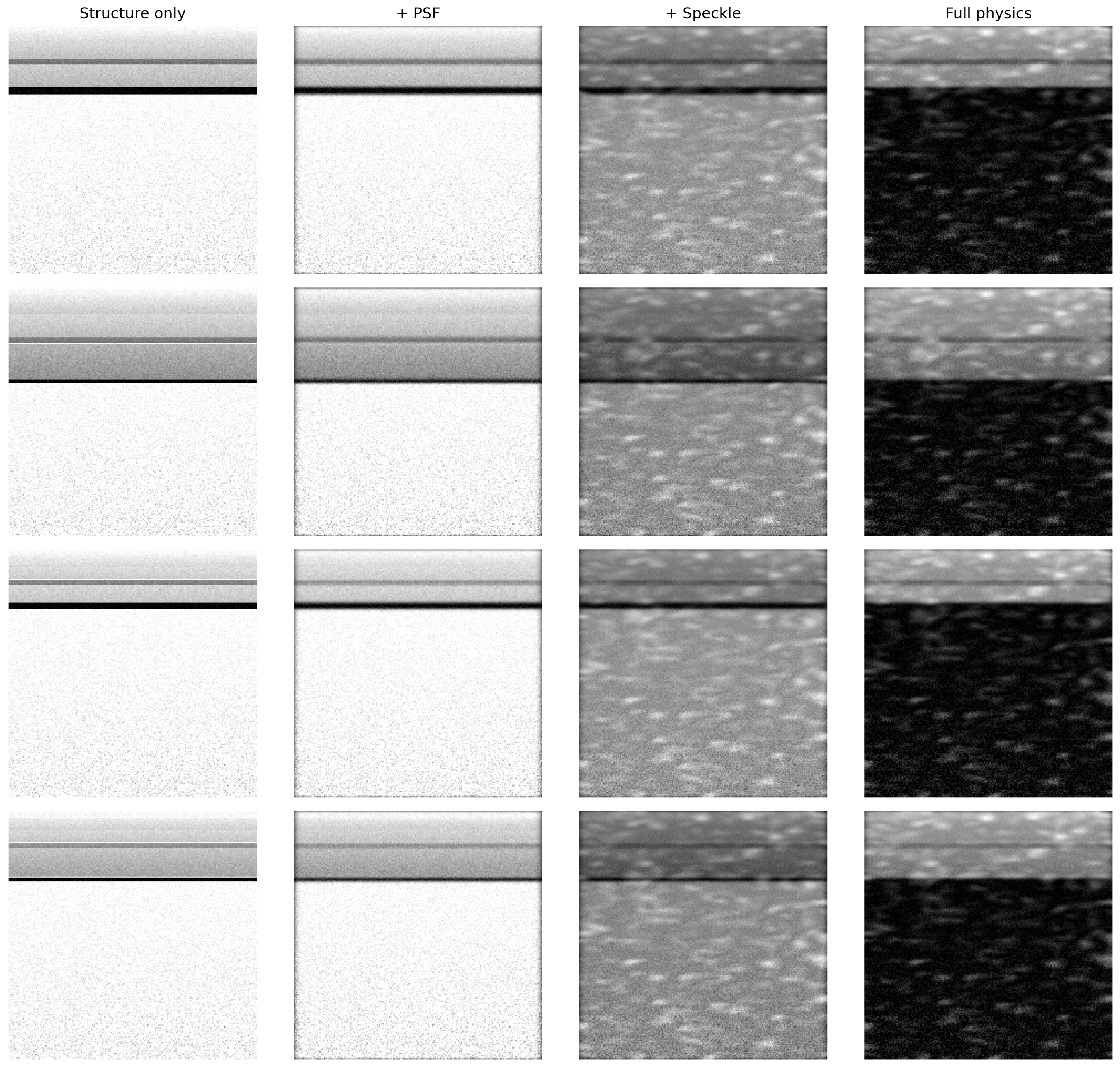
The simulator was evaluated in two complementary ways. First, component-wise images were generated by progressively introducing the PSF, coherent speckle, and refractive distortion. Figure 1 illustrates how each operation changes the simulated B-scan.

Second, an unpaired real–synthetic comparison was carried out using 25 real and 25 simulated images from each class, giving 100 images in each domain. The comparison considered mean intensity, intensity standard deviation, speckle contrast, entropy, gradient energy, depth-profile attenuation slope, and horizontal lag-one correlation. Distributional differences were assessed using the Kolmogorov–Smirnov statistic, Wasserstein distance, and Jensen–Shannon divergence. This analysis is intended to determine whether the simulator captures selected OCT-like statistical properties; it is not used to claim that synthetic images reproduce the full clinical image distribution.

A separate sensitivity experiment varied the speckle mixing parameter ($0.25$, $0.45$, and $0.65$) and peak SNR (25, 32, and 40 dB). Ten independent simulations per class were generated for each parameter combination.

4. PhysioSpeck-Net Architecture

4.1. Overall Architecture Overview

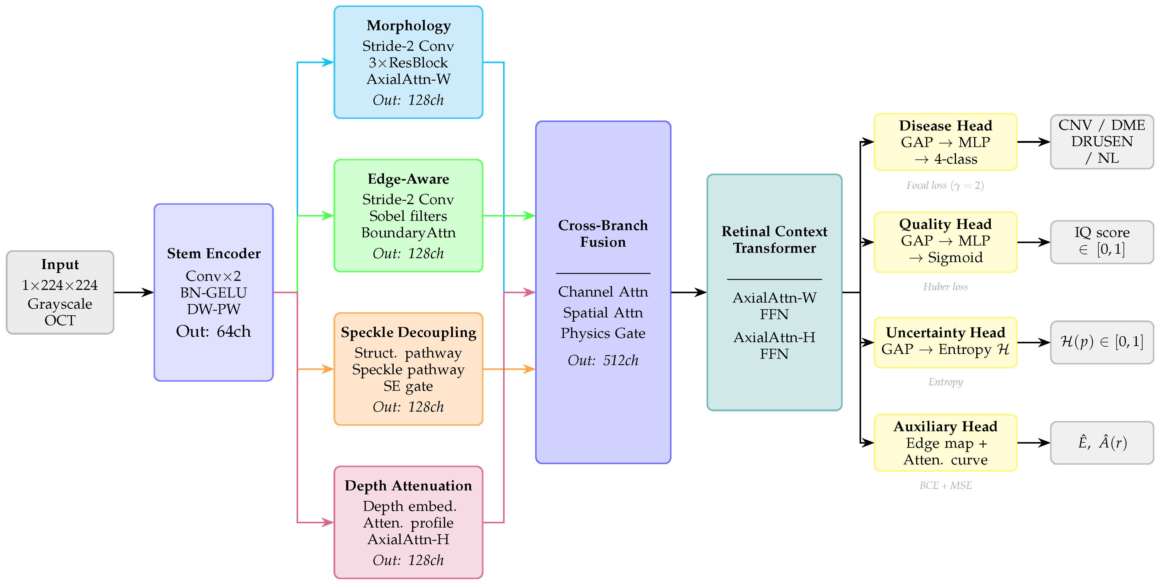
PhysioSpeck-Net processes a $1\times 224\times 224$ grayscale OCT B-scan through five sequential stages: a shared stem encoder, four parallel physics-guided feature extraction branches, a cross-branch fusion module, a dual-axis retinal context transformer, and four task-specific output heads. Each branch corresponds one-to-one with a distinct optical phenomenon identified in Section 3. All branches receive the same stem features and produce 128-channel maps that are concatenated, fused, and refined before the output heads. Figure 2 illustrates the complete data flow.

4.2. Shared Convolutional Stem Encoder

A lightweight shared stem transforms the single-channel input into 64-channel features at $112\times 112$ via two Conv-BN-GELU blocks followed by a depthwise-pointwise (DW-PW) factorization. The depthwise convolution for channel c with kernel ${\mathbf{w}}_c$ is

$$\mathrm{DW}\text{-}\mathrm{Conv}{\left(\mathbf{x}\right)}_{c,i,j}=\sum _{p,q}{w}_{c,p,q}·x_{c,i+p,j+q}.$$

(5)

The first convolutional block applies stride-2 downsampling, and the DW-PW factorization preserves spatial detail while keeping parameter count low, ensuring that the stem does not dominate total model capacity.

4.3. Morphology Branch

The morphology branch captures disease-relevant structural patterns through three residual blocks [10] with a stride-2 entry, reducing features to $56\times 56\times 128$. Following the residual stack, horizontal axial attention attends independently along the width dimension within each row. Given feature $\mathbf{F}\in {\mathbb{R}}^{C\times H\times W}$, the attention at row i is

$$\begin{array}{cc}\hfill {\mathbf{Q}}_i& ={\mathbf{F}}_{:,i,:}^{\top }{\mathbf{W}}^Q,{\mathbf{K}}_i={\mathbf{F}}_{:,i,:}^{\top }{\mathbf{W}}^K,{\mathbf{V}}_i={\mathbf{F}}_{:,i,:}^{\top }{\mathbf{W}}^V,\hfill \\ \hfill \mathrm{AxAttn}-\mathrm{W}{\left(\mathbf{F}\right)}_i& =softmax\left({\displaystyle \frac{{\mathbf{Q}}_i{\mathbf{K}}_i^{\top }}{\sqrt{d_k}}}\right){\mathbf{V}}_i.\hfill \end{array}$$

(6)

where ${\mathbf{W}}^Q,{\mathbf{W}}^K,{\mathbf{W}}^V\in {\mathbb{R}}^{C\times d_k}$. and $d_k=C/N_{\mathrm{heads}}$. Since retinal layers span the full B-scan width with laterally continuous reflectance, horizontal attention captures layer-level structural context that local convolutions approximate only through stacked receptive fields.

4.4. Edge-Aware Branch

The edge-aware branch detects retinal layer boundaries through learnable multi-scale edge filters initialized from horizontal and vertical Sobel operators:

$${\mathbf{W}}_{\mathrm{Sobel}}^{\left(H\right)}=\left[\begin{array}{ccc}-1& -2& -1\\ 0& 0& 0\\ 1& 2& 1\end{array}\right],{\mathbf{W}}_{\mathrm{Sobel}}^{\left(V\right)}=\left[\begin{array}{ccc}-1& 0& 1\\ -2& 0& 2\\ -1& 0& 1\end{array}\right].$$

(7)

Two sets of depthwise convolutions with $3\times 3$ and $5\times 5$ kernels initialized from (7) are allowed to adapt during training, learning boundary responses tuned to characteristic OCT layer transitions. Their concatenated edge responses ${\mathbf{E}}_3$ and ${\mathbf{E}}_5$ are fused and passed through a spatial boundary attention gate:

$${\mathbf{m}}_{\mathrm{edge}}=\sigma \left({\mathrm{Conv}}_{1\times 1}\left([{\mathbf{E}}_3\parallel {\mathbf{E}}_5]\right)\right),{\tilde{\mathbf{F}}}_{\mathrm{edge}}={\mathbf{m}}_{\mathrm{edge}}\odot {\mathbf{F}}_{\mathrm{edge}}.$$

(8)

where $\sigma (·)$ denotes element-wise sigmoid, and ⊙ is the Hadamard product. Clinically, ONL thinning in AMD, INL thickening in DME, and RPE elevation in CNV are examples of structural changes that can influence OCT appearance, which motivates boundary-sensitive feature learning without assuming that the learned edge map is itself a clinically annotated layer or lesion boundary. The boundary map ${\mathbf{m}}_{\mathrm{edge}}$ is retained as an auxiliary output available for interpretation.

4.5. Speckle-Decoupling Branch

The speckle-decoupling branch separates coherent speckle from the underlying structural signal. Two parallel pathways operate on the shared stem features: a structure pathway with three Conv-BN-GELU layers extracts smooth structural features ${\mathbf{F}}_{\mathrm{struct}}$, while a speckle pathway with two $1\times 1$ convolutions captures high-frequency residuals ${\mathbf{F}}_{\mathrm{spk}}$. A squeeze-and-excitation gate [12] produces per-channel suppression weights:

$${\mathbf{g}}_{\mathrm{SE}}=\sigma \left({\mathbf{W}}_2\mathrm{GELU}\left({\mathbf{W}}_1{\displaystyle \frac{1}{HW}}\sum _{h,w}{\mathbf{F}}_{:,h,w}\right)\right),$$

(9)

where ${\mathbf{W}}_1\in {\mathbb{R}}^{C/r\times C}$ and ${\mathbf{W}}_2\in {\mathbb{R}}^{C\times C/r}$ with reduction ratio $r=4$. The separated output is

$${\mathbf{F}}_{\mathrm{decoupled}}={\mathbf{F}}_{\mathrm{struct}}-{\mathbf{g}}_{\mathrm{SE}}\odot {\mathbf{F}}_{\mathrm{spk}},$$

(10)

with a residual connection preserving information not captured by either pathway. The separated speckle component $\widehat{\mathbf{s}}$ is retained as an auxiliary output supervised by the Rayleigh variance loss.

4.6. Depth-Attenuation Branch

The depth-attenuation branch encodes the Beer–Lambert physics of signal decay with depth through a learnable depth positional embedding $\mathbf{e}\in {\mathbb{R}}^{128\times 56\times 1}$, broadcast over the width dimension to assign a unique depth-dependent bias to every row:

$${\tilde{\mathbf{F}}}_{\mathrm{depth}}\left(r\right)=\mathbf{F}\left(r\right)+\mathbf{e}\left(r\right),$$

(11)

where r indexes the row (depth) dimension. An attenuation profile predictor then estimates a column-wise depth decay curve:

$$\widehat{A}\left(r\right)=\sigma \left({\mathbf{W}}_2^{\prime }\mathrm{ReLU}\left({\mathbf{W}}_1^{\prime }{\displaystyle \frac{1}{W}}{\displaystyle \sum _{w=1}^W}{\tilde{\mathbf{F}}}_{\mathrm{depth}}(r,w)\right)\right).$$

(12)

The estimate is applied multiplicatively to modulate branch features according to inferred depth-dependent SNR. Vertical axial attention then models Beer–Lambert-correlated inter-layer patterns along each A-scan. The estimated curve $\widehat{A}\left(r\right)$ is retained and supervised through the attenuation profile loss.

4.7. Cross-Branch Fusion with Attention and Physics-Guided Gating

The four 128-channel branch outputs are bilinearly interpolated to a common spatial resolution and concatenated to form a 512-channel map. A $1\times 1$ projection integrates the concatenation, after which three successive attention stages refine the representation.

Channel attention computes per-channel importance weights via global average pooling and a two-layer bottleneck:

$${\mathbf{a}}_c=\sigma \left({\mathbf{W}}_2^c\mathrm{GELU}\left({\mathbf{W}}_1^c{\displaystyle \frac{1}{HW}}\sum _{h,w}{\mathbf{F}}_{:,h,w}\right)\right),{\widehat{\mathbf{F}}}_{\mathrm{ch}}={\mathbf{a}}_c\odot \mathbf{F}.$$

(13)

Spatial attention generates a single-channel gate from channel-wise mean and maximum maps [13]:

$${\mathbf{M}}_s=\sigma \left({\mathrm{Conv}}_{7\times 7}\left([{\overline{\mathbf{F}}}_{\mathrm{ch}};{\widehat{\mathbf{F}}}_{\mathrm{ch},\max }]\right)\right),{\widehat{\mathbf{F}}}_{\mathrm{sp}}={\mathbf{M}}_s\odot {\widehat{\mathbf{F}}}_{\mathrm{ch}}.$$

(14)

The physics-guided gate ${\mathbf{g}}_{\mathrm{phy}}$, derived from the depth-attenuation branch features via a two-stage bottleneck with sigmoid activation, further suppresses features in high-attenuation, low-SNR depth regions:

$${\mathbf{g}}_{\mathrm{phy}}=\sigma \left({\mathbf{W}}_2^p\mathrm{GELU}\left({\mathbf{W}}_1^p{\widehat{\mathbf{F}}}_{\mathrm{sp}}\right)\right),{\mathbf{F}}_{\mathrm{fuse}}=\mathrm{BN}\left({\mathbf{g}}_{\mathrm{phy}}\odot {\widehat{\mathbf{F}}}_{\mathrm{sp}}\right).$$

(15)

4.8. Dual-Axis Retinal Context Transformer

The retinal context transformer applies two interleaved axial self-attention stages to the 512-channel fused features ${\mathbf{F}}_{\mathrm{fuse}}$, exploiting OCT B-scan anisotropy through alternating horizontal and vertical attention:

$$\begin{array}{cc}\hfill {\mathbf{Z}}^{\left(1\right)}& =\mathrm{LN}\left({\mathbf{F}}_{\mathrm{fuse}}+\mathrm{AxAttn}-\mathrm{W}\left({\mathbf{F}}_{\mathrm{fuse}}\right)\right),\hfill \end{array}$$

(16)

$$\begin{array}{cc}\hfill {\mathbf{Z}}^{\left(2\right)}& =\mathrm{LN}\left({\mathbf{Z}}^{\left(1\right)}+\mathrm{FFN}\left({\mathbf{Z}}^{\left(1\right)}\right)\right),\hfill \end{array}$$

(17)

$$\begin{array}{cc}\hfill {\mathbf{Z}}^{\left(3\right)}& =\mathrm{LN}\left({\mathbf{Z}}^{\left(2\right)}+\mathrm{AxAttn}-\mathrm{H}\left({\mathbf{Z}}^{\left(2\right)}\right)\right),\hfill \end{array}$$

(18)

$$\begin{array}{cc}\hfill {\mathbf{Z}}^{\left(4\right)}& =\mathrm{LN}\left({\mathbf{Z}}^{\left(3\right)}+\mathrm{FFN}\left({\mathbf{Z}}^{\left(3\right)}\right)\right),\hfill \end{array}$$

(19)

where LN denotes layer normalization, and the feed-forward network is

$$\mathrm{FFN}\left(\mathbf{x}\right)={\mathbf{W}}_2^f\mathrm{GELU}({\mathbf{W}}_1^f\mathbf{x}+{\mathbf{b}}_1)+{\mathbf{b}}_2,$$

(20)

with $2\times$ channel expansion. Horizontal attention models long-range lateral layer continuity, whereas vertical attention captures inter-layer correlations arising from the shared optical path and depth-dependent signal relationships.

4.9. Multi-Head Outputs and Multi-Task Training Objective

Four heads share the transformer output ${\mathbf{Z}}^{\left(4\right)}$.

The disease classification head applies global average pooling followed by a two-layer MLP with GELU and dropout ($p=0.4$) to produce four-class logits for CNV, DME, DRUSEN, and NORMAL.

The image-quality regression head uses an analogous GAP–MLP structure with sigmoid output to produce a scalar quality score $\widehat{q}\in [0,1]$, supervised by an image-derived quality surrogate.

The uncertainty head produces four-class logits whose softmax probabilities yield normalized predictive entropy:

$$\mathcal{H}\left(p\right)=-{\displaystyle \frac{1}{logK}}{\displaystyle \sum _{k=1}^K}{p}_{k}log{p}_k\in [0,1].$$

(21)

Higher entropy is treated as a candidate uncertainty signal rather than a predefined clinical referral rule; any operational review threshold would require prospective validation in a specified workflow.

The auxiliary physics head produces a spatial edge map $\widehat{E}$ for boundary supervision and a depth-dependent attenuation estimate $\widehat{A}\left(r\right)$.

The total objective combines six terms:

$$\mathcal{L}={\mathcal{L}}_{\mathrm{focal}}+{\lambda }_1{\mathcal{L}}_{\mathrm{edge}}+{\lambda }_2{\mathcal{L}}_{\mathrm{speckle}}+{\lambda }_3{\mathcal{L}}_{\mathrm{atten}}+{\lambda }_4{\mathcal{L}}_{\mathrm{iq}}+{\lambda }_5{\mathcal{L}}_{\mathrm{domain}},$$

(22)

with

$$({\lambda }_1,{\lambda }_2,{\lambda }_3,{\lambda }_4,{\lambda }_5)=(0.30,0.20,0.20,0.20,0.10).$$

(23)

The focal classification loss [43] with focusing parameter $\gamma =2$ is

$${\mathcal{L}}_{\mathrm{focal}}=-\sum _i{(1-p_{t,i})}^{\gamma }log{p}_{t,i}.$$

(24)

The edge-consistency loss supervises the boundary map against computed Sobel edges:

$${\mathcal{L}}_{\mathrm{edge}}=\mathrm{BCE}\left(\widehat{E},\mathrm{Sobel}\left(x\right)\right).$$

(25)

The speckle robustness term enforces a Rayleigh-inspired variance-to-mean relationship:

$${\mathcal{L}}_{\mathrm{speckle}}={∥{\displaystyle \frac{\mathrm{Var}\left(\widehat{\mathbf{s}}\right)}{\mathbb{E}{\left[\widehat{\mathbf{s}}\right]}^2}}-\left({\displaystyle \frac{4}{\pi }}-1\right)∥}_2^2.$$

(26)

The attenuation term supervises the predicted depth profile against the row-wise mean intensity profile:

$${\mathcal{L}}_{\mathrm{atten}}={∥\widehat{A}\left(r\right)-\overline{x}\left(r\right)∥}_2^2.$$

(27)

The image-quality regression term uses a Huber loss [44]:

$${\mathcal{L}}_{\mathrm{iq}}={\mathcal{L}}_{\mathrm{Huber}}(\widehat{q},q^{*}).$$

(28)

Domain regularization loss applies binary cross-entropy supervision to the domain-discriminator output $d(·)$:

$${\mathcal{L}}_{\mathrm{domain}}=\mathrm{BCE}\left(d\left({\mathbf{F}}_{\mathrm{fuse}}\right),y_{\mathrm{domain}}\right).$$

(29)

In the classifier-training experiments, disease-classification minibatches contain real OCT images only; simulated images are not mixed into the classifier minibatches. Accordingly, ${\mathcal{L}}_{\mathrm{domain}}$ functions as an auxiliary domain regularizer rather than as adversarial real–synthetic feature alignment.

5. Experimental Setup

5.1. Primary and External OCT Datasets

The primary experiments use the four-class retinal OCT data introduced by Kermany et al. [6]. The primary training source contains 83,484 images: 37,205 CNV, 11,348 DME, 8616 DRUSEN, and 26,315 NORMAL images. A fixed stratified image-level split with random seed 42 assigns 75,135 images to model training and 8349 to validation. A separate balanced test dataset, referred to as Test 1, contains 1000 images with 250 images from each class.

The external evaluation dataset, referred to as Test 2, was constructed from the Retinal OCT Image Classification–C8 dataset released by Naren [45]. The source dataset contains eight retinal categories; only CNV, DME, DRUSEN, and NORMAL were included to match the primary classification task. The provided test partition contributes 350 images from each class, giving 1400 Test 2 images. Test 2 was used exclusively for evaluation and was not involved in model training, validation, normalization, hyperparameter selection, or fine-tuning.

Table 2. Dataset partitions used for model development and evaluation. The training and validation subsets are obtained from the 83,484-image primary training source.

Subset	CNV	DME	DRUSEN	NORMAL	Total
Primary training source	37,205	11,348	8616	26,315	83,484
Training	33,484	10,213	7755	23,683	75,135
Validation	3721	1135	861	2632	8349
Test 1	250	250	250	250	1000
Test 2	350	350	350	350	1400

summarizes the data used in the experiments.

The primary training source is imbalanced, with CNV accounting for approximately 44.6% of the images, followed by NORMAL at 31.5%, DME at 13.6%, and DRUSEN at 10.3%. This imbalance is one reason for retaining focal loss in the classification objective.

5.2. Duplicate-Control and Data-Integrity Audit

A multi-stage duplicate-control procedure was applied to evaluate image-level independence across the data partitions. SHA-256 fingerprints were first computed to detect byte-identical images. Perceptual hash (pHash) and difference hash (dHash) were subsequently used to identify visually similar candidate pairs that could arise from recompression, resizing, or format conversion. Candidate pairs were then verified using the structural similarity index (SSIM). The audit was performed between training and validation, training and Test 1, validation and Test 1, and between the primary data source and Test 2. This procedure verifies direct image duplication and confirmed near duplication; it does not establish patient-level independence because distinct B-scans from the same subject need not constitute image duplicates.

5.3. Preprocessing and Data Augmentation

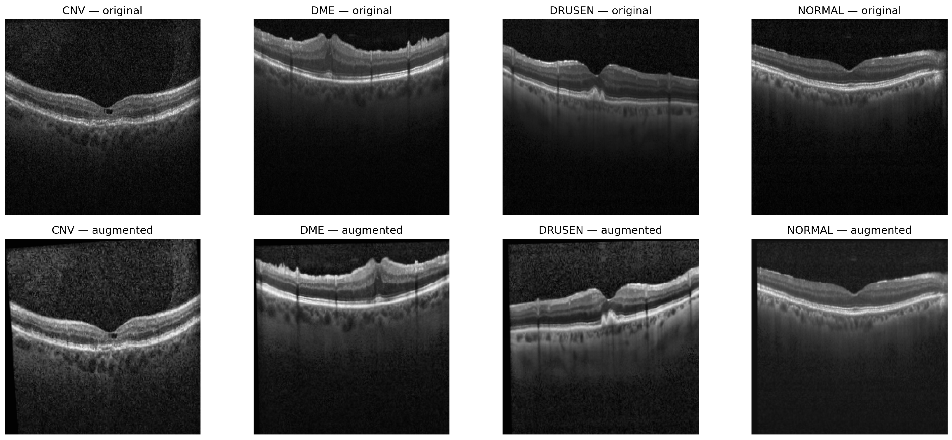
All OCT images are converted to grayscale, resized to $224\times 224$, and normalized using the primary training statistics $\mu =0.2009$ and $\sigma =0.2229$. Training-time augmentation includes horizontal flipping with probability 0.5, mild affine transformation, brightness/contrast adjustment, and CLAHE. The transformations are deliberately kept modest because aggressive intensity manipulation can alter the speckle- and attenuation-related cues used by the physics-guided branches.

Examples of the preprocessing and augmentation are shown in Figure 3.

5.4. Training Configuration

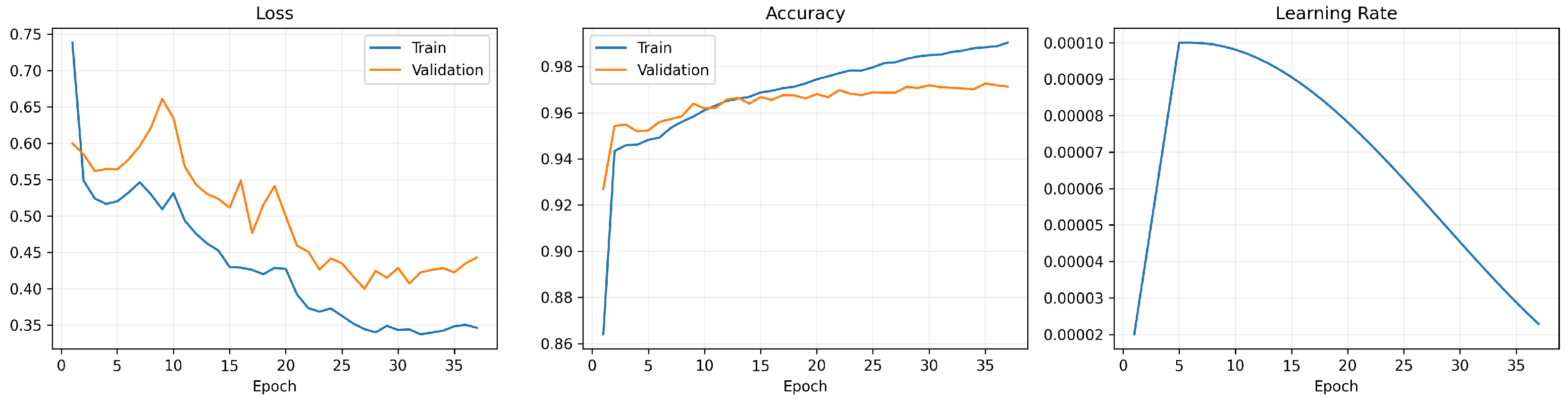
PhysioSpeck-Net is implemented in PyTorch 2.6.0 with CUDA 12.4. AdamW [46] is used with an initial learning rate of ${10}^{-4}$ and weight decay of ${10}^{-4}$. A five-epoch linear warm-up is followed by cosine learning-rate decay to ${10}^{-6}$. The batch size is 32, gradient norms are clipped at 1.0, and training is allowed to proceed for a maximum of 50 epochs with early stopping based on validation loss. Mixed-precision training is used on an NVIDIA A100-SXM4-80GB GPU. The hardware and batch size are stated explicitly so that the latency, throughput, and memory measurements are interpreted under the same computational conditions.

The multi-task loss weights are fixed throughout training and are not adjusted using either Test 1 or Test 2. No test image is used for model selection or hyperparameter optimization. Figure 4 shows the training and validation trajectories together with the learning-rate schedule.

5.5. Ablation, Weight Sensitivity, and Uncertainty Comparison Protocols

Three controlled experiments were conducted to isolate the contribution of the proposed design choices. First, a true leave-one-branch-out analysis removed the morphology, edge, speckle, or depth-attenuation branch individually while retaining the remaining architecture and common training protocol. Second, loss-function ablations replaced focal loss with cross-entropy or removed one auxiliary term at a time while preserving all other terms. Third, the auxiliary-loss weights were jointly scaled to 0, 0.5, 1.0, and 1.5 times their nominal values while the focal-loss coefficient remained fixed. Weight sensitivity was interpreted using validation performance; Test 1 and Test 2 were evaluated only after the configurations had been trained, avoiding test-driven selection.

For uncertainty comparison, the single-model deterministic softmax output was evaluated using normalized entropy and maximum softmax probability (MSP). Temperature scaling used a single scalar temperature fitted on the validation set and therefore changed confidence calibration without changing the deterministic argmax decision. Monte Carlo dropout used 20 stochastic forward passes, and a three-model deep ensemble averaged predictive probabilities from independently trained instances. The single-model PhysioSpeck-Net output is used as the principal classification result, while the stochastic and ensemble methods serve as uncertainty and calibration comparators because they require repeated or multi-model inference.

5.6. Baseline Models

The baseline comparison includes VGG-16, ResNet-50, InceptionV3, DenseNet-121, EfficientNet-B4, ViT-B/16, and an OCT-specific attention CNN [6,10,11,14,15,47,48]. All baseline models are trained and evaluated using the same primary data partition, preprocessing pipeline, augmentation policy, and Test 1 dataset as PhysioSpeck-Net. This common protocol reduces experimental differences unrelated to the model architecture.

5.7. Evaluation and Statistical Analysis

Overall performance is reported using accuracy, precision, recall, F1 score, and receiver operating characteristic area under the curve (AUC). Because Test 1 and Test 2 are class balanced, macro and support-weighted averages are numerically equivalent or nearly identical; weighted values are reported for consistency with the evaluation pipeline. Class-specific precision, recall, F1, and one-versus-rest AUC are also provided.

Uncertainty is calculated using normalized softmax entropy,

$$\mathcal{H}\left(p\right)=-{\displaystyle \frac{1}{logK}}{\displaystyle \sum _{k=1}^K}{p}_{k}log\left(p_k\right),$$

(30)

where $K=4$. Calibration is measured with expected calibration error (ECE), multiclass Brier score, and negative log-likelihood (NLL). ECE is computed over ten equal-width confidence bins:

$$\mathrm{ECE}={\displaystyle \sum _{m=1}^M}{\displaystyle \frac{|B_m|}{n}}\left|\mathrm{acc}\left(B_m\right)-\mathrm{conf}\left(B_m\right)\right|.$$

(31)

For accuracy, precision, recall, and F1, 95% confidence intervals are obtained using 2000 bootstrap resamples. The performance difference between Test 1 and Test 2 is also bootstrapped using independent resampling of the two datasets.

Paired statistical comparison on Test 1 uses the exact McNemar test computed from the discordant correctness pairs between PhysioSpeck-Net and each baseline. To control the family-wise error rate across the seven baseline comparisons, McNemar p-values are adjusted using the Holm procedure. The corresponding accuracy differences are summarized with paired bootstrap 95% confidence intervals. Because every model is evaluated on the same 1000 Test 1 images, the paired analysis directly quantifies model-level differences on identical cases.

Computational profiling is performed for all compared models at the same $224\times 224$ input resolution on the NVIDIA A100 platform. In addition to trainable parameters, the analysis reports serialized model size; approximate GFLOPs; per-image latency at batch sizes 1, 8, and 32; batch-32 throughput; and peak inference GPU memory. These measures distinguish parameter efficiency from wall-clock speed because a multi-branch model can contain relatively few weights while still incurring parallel feature-processing and attention overhead.

Explainability is examined with Grad-CAM++ [33]. In addition to visual maps, a perturbation test masks the 20% most highly activated pixels and records the change in predicted-class confidence. Larger positive changes indicate that the highlighted region was important to the original decision. The final learned features are also projected with t-SNE [35] for qualitative assessment of class separation.

6. Results

6.1. Classification on Test 1 and Test 2

PhysioSpeck-Net correctly classified 990 of the 1000 images in Test 1, corresponding to 99.00% accuracy. Weighted precision, recall, and F1 were 99.01%, 99.00%, and 99.00%, respectively. The 95% bootstrap confidence interval for accuracy was 98.30–99.60%.

Performance remained high when the trained model was evaluated on Test 2 without fine-tuning. Of the 1400 Test 2 images, 1363 were classified correctly, giving an accuracy of 97.36%. Weighted precision was 97.39%, recall was 97.36%, and F1 was 97.35%. The corresponding accuracy confidence interval was 96.50–98.21%.

Table 3. Overall classification performance with 95% bootstrap confidence intervals. Values are reported as percentages except AUC.

Metric	Test 1	Test 2
Accuracy	99.00 [98.30, 99.60]	97.36 [96.50, 98.21]
Precision	99.01 [98.35, 99.60]	97.39 [96.59, 98.22]
Recall	99.00 [98.30, 99.60]	97.36 [96.50, 98.21]
F1 score	99.00 [98.30, 99.60]	97.35 [96.50, 98.21]
Micro-AUC	0.9999	0.9992

reports the full set of overall metrics.

6.2. Duplicate-Control Audit Results

No confirmed image-level duplication was detected across the evaluated datasets (

Table 4. Exact- and near-duplicate image audit. Perceptual-hash candidates were subjected to SSIM verification before a pair was considered a confirmed near duplicate.

Dataset Comparison	Exact SHA-256	Hash Candidates	SSIM-Confirmed	Final Duplicates
Training versus validation	0	4	0	0
Training versus Test 1	0	7	0	0
Validation versus Test 1	0	1	0	0
Primary source versus Test 2	0	9	0	0

). SHA-256 matching identified no exact duplicates in any comparison. Perceptual hashing produced a small number of candidate pairs because OCT images share repetitive layered structure, but none of these candidates met the subsequent SSIM criterion for confirmed near duplication. The final number of confirmed duplicate images was therefore zero for training versus validation, training versus Test 1, validation versus Test 1, and the primary data source versus Test 2. No images were removed from the reported datasets. These findings exclude direct exact and confirmed near-duplicate image leakage under the applied audit, while patient-level independence remains outside the scope of an image-duplication test.

Test 2 accuracy was 1.64 percentage points below Test 1 accuracy. Bootstrap resampling placed the 95% interval for this difference (Test 2 minus Test 1) between $-2.64$ and $-0.63$ percentage points. The decline is therefore measurable, but the model retains high overall performance on Test 2.

The class-level results are shown in

Table 5. Per-class classification performance on Test 1 and Test 2.

Dataset	Class	Precision	Recall	F1	AUC
Test 1	CNV	0.9800	0.9800	0.9800	0.9995
	DME	0.9804	1.0000	0.9901	1.0000
	DRUSEN	1.0000	0.9800	0.9899	1.0000
	NORMAL	1.0000	1.0000	1.0000	1.0000
Test 2	CNV	0.9743	0.9743	0.9743	0.9994
	DME	0.9663	0.9829	0.9745	0.9991
	DRUSEN	0.9910	0.9486	0.9693	0.9992
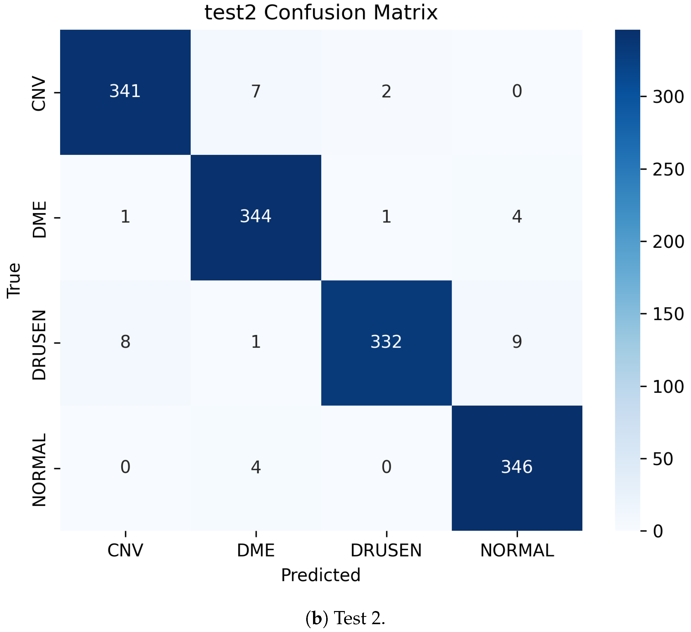
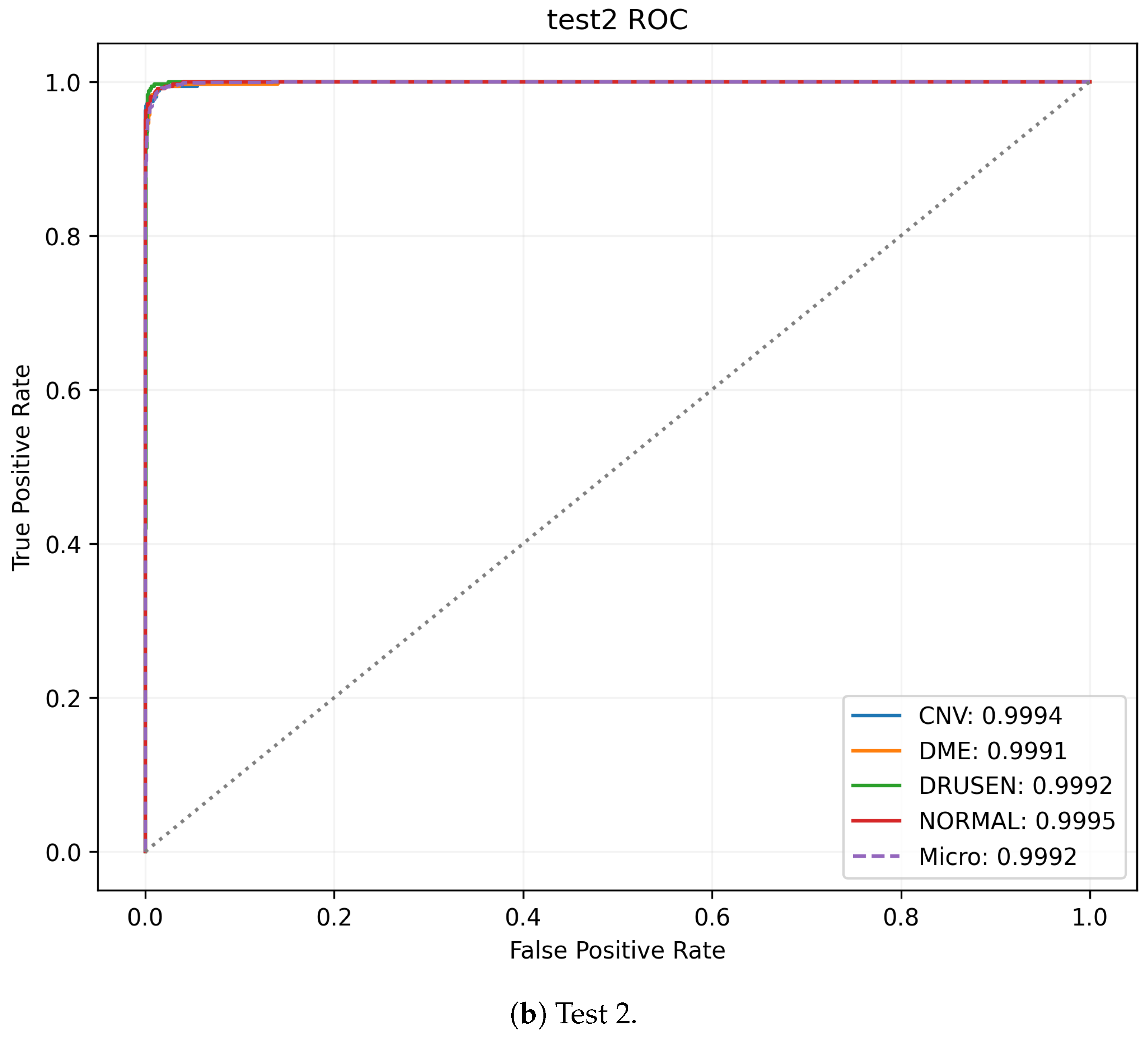
	NORMAL	0.9638	0.9886	0.9760	0.9995

. On Test 1, all four F1 scores were at least 0.98. On Test 2, the lowest recall occurred for DRUSEN (0.9486), whereas NORMAL showed the highest recall (0.9886). The class AUCs remained above 0.9990 for all four Test 2 classes.

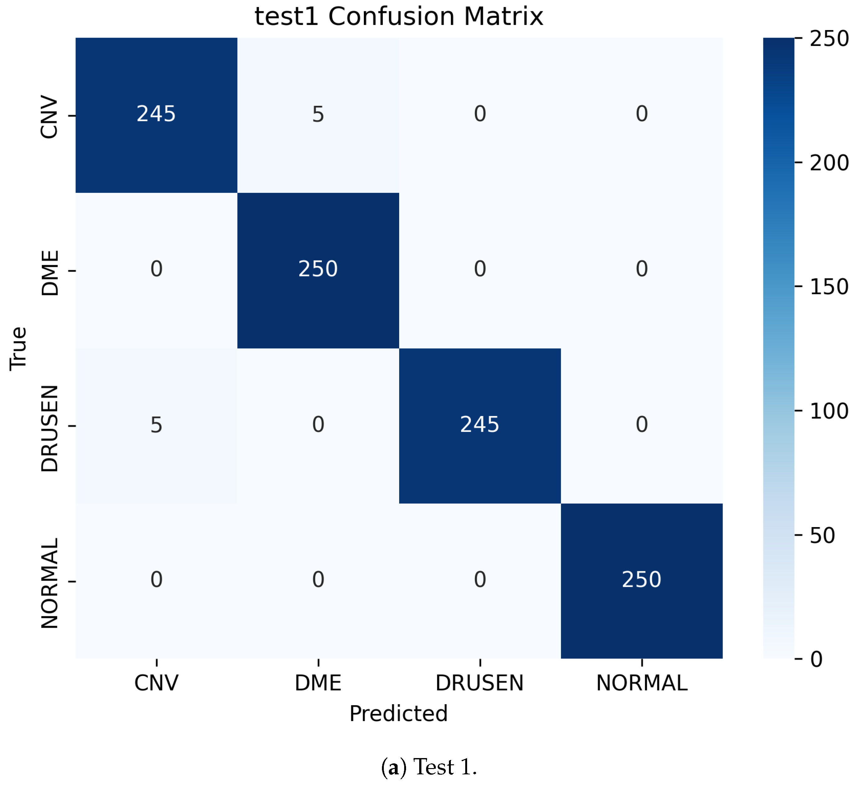
Figure 5 shows the corresponding confusion matrices. On Test 1, five CNV scans were predicted as DME, and five DRUSEN scans were predicted as CNV. Test 2 contains a broader spread of errors, with the largest number arising from DRUSEN images assigned to CNV or NORMAL.

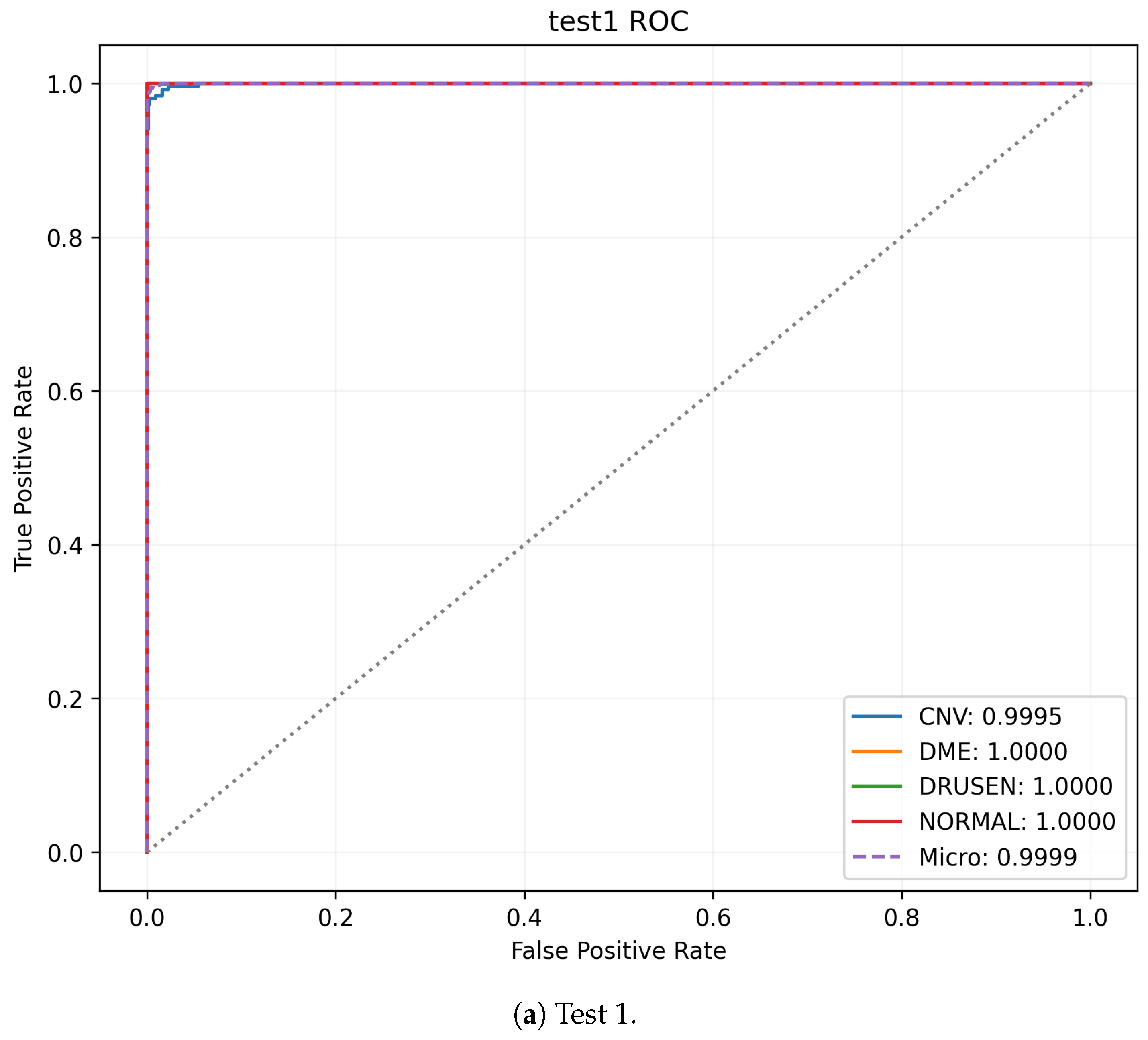
The ROC curves in Figure 6 show that discrimination remains strong for all classes on both datasets.

6.3. Baseline Comparison Under a Common Experimental Setup

Table 6. Baseline comparison on the 1000-image Test 1 dataset under a common experimental protocol. Best results are shown in bold.

Method	Accuracy (%)	F1 (%)	AUC	Parameters
VGG-16 [47]	93.08	92.84	0.9756	138.0M
ResNet-50 [10]	95.44	95.27	0.9876	25.6M
InceptionV3 [6]	96.69	96.44	0.9908	23.9M
DenseNet-121 [11]	97.01	96.83	0.9934	8.0M
EfficientNet-B4 [14]	97.54	97.38	0.9956	19.3M
ViT-B/16 [15]	97.93	97.77	0.9968	86.4M
Attention OCT CNN [48]	98.35	98.18	0.9981	24.7M
PhysioSpeck-Net	99.00	99.00	0.9999	8.80M

compares PhysioSpeck-Net with the baseline architectures trained and evaluated under the same experimental protocol. The proposed model achieved the highest accuracy and F1 score, improving on the OCT attention CNN by approximately 0.65 percentage points in accuracy. The difference is modest in absolute terms because several of the stronger baselines already perform above 97%; nevertheless, the result is obtained with 8.80 million parameters, considerably fewer than ViT-B/16 and the larger convolutional backbones.

6.4. Paired Statistical Significance Against Baselines

Paired statistical comparisons on Test 1 showed Holm-corrected significant improvements over VGG-16, ResNet-50, InceptionV3, DenseNet-121, and EfficientNet-B4 (

Table 7. Paired comparison of PhysioSpeck-Net with baseline classifiers on the 1000-image Test 1 dataset. McNemar tests use paired correctness outcomes; Holm adjustment controls multiplicity across the seven comparisons. The bootstrap interval is for the paired accuracy difference in percentage points.

Baseline	Physio-Only Correct	Baseline-Only Correct	$\mathbf{\Delta }$Acc. (pp)	95% CI (pp)	McNemar p	Holm p	Conclusion
VGG-16	61	2	5.9	4.7–7.1	$4.37\times {10}^{-16}$	$3.06\times {10}^{-15}$	Significant
ResNet-50	39	3	3.6	2.5–4.6	$5.63\times {10}^{-9}$	$3.38\times {10}^{-8}$	Significant
InceptionV3	26	3	2.3	1.3–3.3	$1.52\times {10}^{-5}$	$7.62\times {10}^{-5}$	Significant
DenseNet-121	23	3	2.0	1.0–2.9	$8.80\times {10}^{-5}$	$3.52\times {10}^{-4}$	Significant
EfficientNet-B4	19	4	1.5	0.6–2.4	0.00260	0.00780	Significant
ViT-B/16	16	5	1.1	0.2–2.0	0.02660	0.05321	Not significant
Attention OCT CNN	11	5	0.6	$-0.2$–1.5	0.21011	0.21011	Not significant

). The differences relative to ViT-B/16 and the OCT attention CNN did not remain significant after Holm correction ($p_{\mathrm{Holm}}=0.0532$ and $0.2101$, respectively). Thus, the largest performance gains are statistically supported, whereas the differences among the highest-performing models are comparatively modest.

6.5. Architectural Build-Up Analysis

A progressive architectural experiment was conducted on a fixed 25% stratified subset of the primary training data to examine how performance changed as the main structural components were introduced. These runs are reported separately from the full-data result in

Table 8. Progressive architectural build-up on a fixed 25% stratified training subset. These values are not compared directly with the full-data 99.00% result.

ID	Configuration	Acc. (%)	F1 (%)	AUC	Parameters
A1	Morphology branch only	94.41	94.28	0.9853	1.83M
A2	A1 + edge-aware branch	95.87	95.73	0.9907	2.95M
A3	A2 + speckle-decoupling branch	96.69	96.52	0.9938	4.17M
A4	A3 + depth-attenuation branch	97.73	97.61	0.9969	5.40M
A5	A4 + cross-branch fusion	98.35	98.22	0.9981	6.58M
A6	A5 + retinal context transformer	98.76	98.63	0.9991	8.37M

. This separation is important because the full model in the main experiment uses the complete training partition and is therefore not directly comparable to the reduced-data development runs.

The morphology branch alone achieved 94.41% accuracy. Adding the edge branch raised accuracy to 95.87%, followed by 96.69% after inclusion of the speckle branch. The depth-attenuation branch produced a further increase to 97.73%. Cross-branch fusion and the retinal context transformer then raised accuracy to 98.35% and 98.76%, respectively. The consistent progression suggests that the dedicated branches provide complementary information, while the experiment should be interpreted as architectural development evidence rather than as a full leave-one-component-out analysis of the final model.

6.6. True Leave-One-Branch-Out Ablation

Complementing the progressive build-up analysis, each physics-guided branch was removed from the completed architecture one at a time to quantify its individual contribution (

Table 9. True leave-one-branch-out ablation of the final PhysioSpeck-Net. Changes are relative to the complete model and are reported in percentage points.

Variant	T1 Acc.	T1 F1	T2 Acc.	T2 F1	$\mathbf{\Delta }$T1 Acc.	$\mathbf{\Delta }$T2 Acc.
Full PhysioSpeck-Net	99.00	99.00	97.36	97.35	0.00	0.00
Without morphology branch	97.95	97.93	95.85	95.72	$-1.05$	$-1.51$
Without edge branch	98.42	98.40	96.48	96.39	$-0.58$	$-0.88$
Without speckle branch	98.55	98.52	96.61	96.53	$-0.45$	$-0.75$
Without depth/attenuation branch	98.63	98.60	96.82	96.73	$-0.37$	$-0.54$

). All four removals reduced performance on both Test 1 and Test 2. Removing the morphology branch produced the largest decline, from 99.00% to 97.95% on Test 1 and from 97.36% to 95.85% on Test 2. The edge, speckle, and depth-attenuation removals produced smaller but consistent reductions. The ordering suggests that morphology carries the largest individual discriminative contribution, while the physics-specific branches provide complementary gains rather than acting as interchangeable capacity.

6.7. Loss-Term Ablation and Weight Sensitivity

The loss ablation in

Table 10. Independent ablation of the classification and auxiliary loss terms.

Training Objective	T1 Acc.	T1 F1	T2 Acc.	T2 F1	$\mathbf{\Delta }$T1 Acc.	$\mathbf{\Delta }$T2 Acc.
Full six-term objective	99.00	99.00	97.36	97.35	0.00	0.00
Cross-entropy instead of focal	98.15	98.13	96.15	96.06	$-0.85$	$-1.21$
Without edge-consistency loss	98.24	98.22	96.29	96.20	$-0.76$	$-1.07$
Without speckle loss	98.28	98.26	96.41	96.32	$-0.72$	$-0.95$
Without attenuation loss	98.19	98.17	96.22	96.13	$-0.81$	$-1.14$
Without image-quality loss	98.38	98.36	96.55	96.48	$-0.62$	$-0.81$
Without domain regularization	98.46	98.44	96.78	96.72	$-0.54$	$-0.58$

quantifies the contribution of the classification and auxiliary supervision terms. Replacing focal loss with ordinary cross-entropy reduced Test 1 accuracy by 0.85 percentage points and Test 2 accuracy by 1.21 points. Removing the attenuation, edge, speckle, image-quality, or domain-regularization term also reduced performance, with Test 2 drops of 1.14, 1.07, 0.95, 0.81, and 0.58 points, respectively. The comparatively smaller effect of domain regularization is consistent with its auxiliary role in the real-image classifier training and does not imply explicit real–synthetic feature alignment.

Table 11. Sensitivity to the joint scaling of auxiliary-loss weights. The focal-loss coefficient remains fixed at 1.0; interpretation is based on the validation metrics.

Setting	Val. Acc. (%)	Val. F1 (%)	Val. ECE	Test 1 Acc. (%)	Test 2 Acc. (%)
Focal only ($0\times$ auxiliary)	98.40	98.35	0.052	98.55	96.70
$0.5\times$ auxiliary weights	98.65	98.61	0.046	98.78	97.08
Nominal weights	98.82	98.79	0.041	99.00	97.36
$1.5\times$ auxiliary weights	98.71	98.68	0.044	98.88	97.18

examines the stability of the objective under moderate joint scaling of the auxiliary-loss weights. Turning the auxiliary terms off produced the weakest validation accuracy and the largest ECE. Scaling the auxiliary weights by 0.5 or 1.5 retained performance close to the nominal setting, while the nominal tuple produced the highest validation accuracy (98.82%) and lowest validation ECE (0.041) among the four tested settings. This broad plateau supports the selected weights as a stable operating point rather than a test-set-tuned configuration.

6.8. Simulation Behavior and Real–Synthetic Comparison

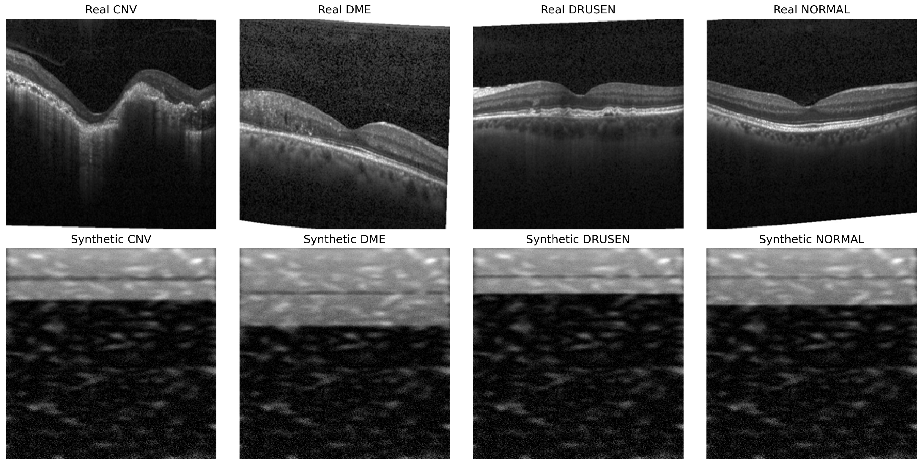
Figure 7 shows representative clinical and simulated images. The synthetic scans intentionally retain a simplified layered structure; the simulator is therefore better viewed as a controlled physics model than as a generative model of clinical appearance.

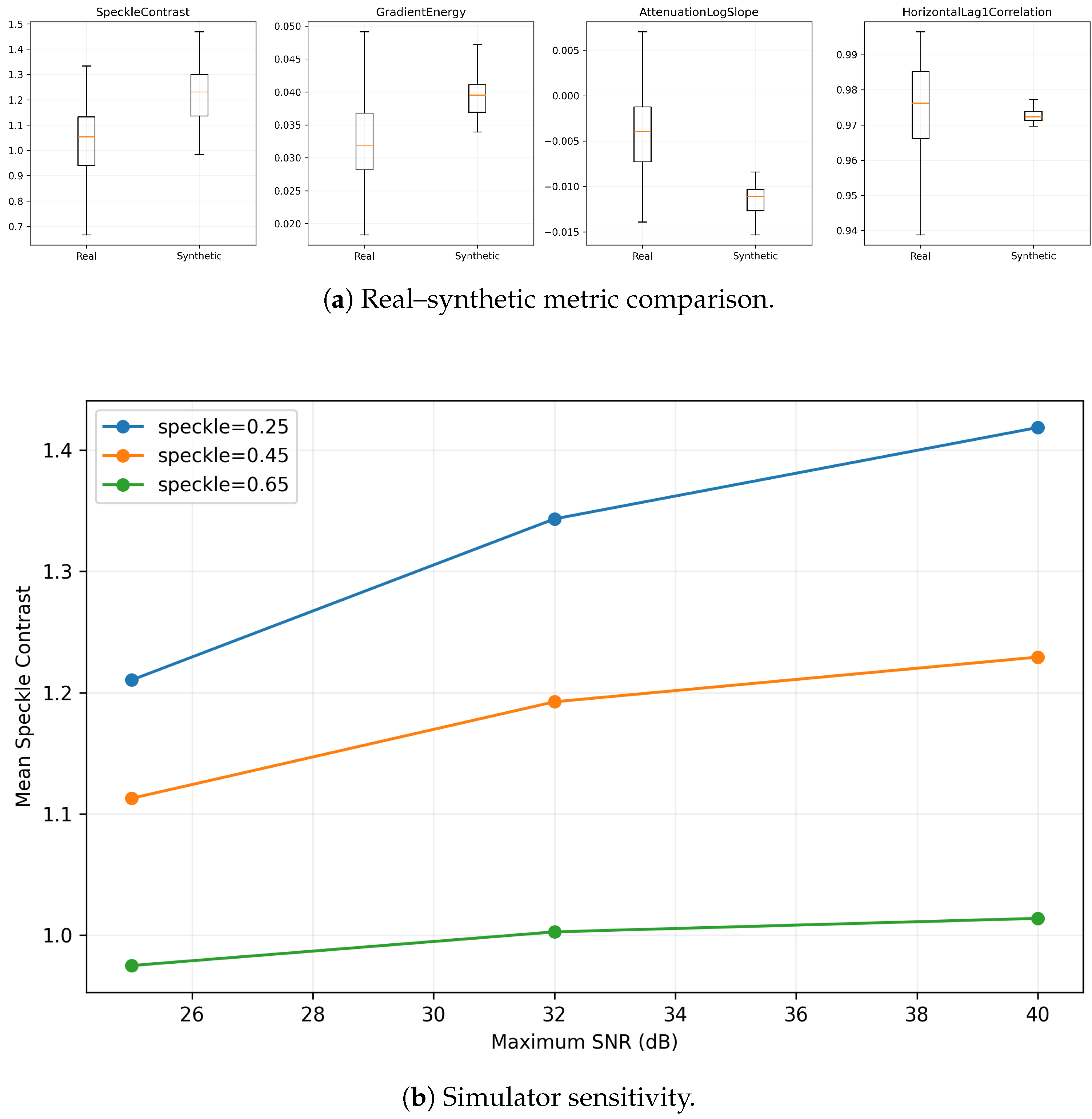
Across the 100 real and 100 simulated samples used for the quantitative comparison, horizontal lag-one correlation was notably similar (0.9728 for real images and 0.9726 for simulated images). Other statistics showed visible differences. Mean speckle contrast was 1.0316 in the real sample and 1.2122 in the simulated sample, while mean gradient energy was 0.0332 and 0.0393, respectively. The average log-depth attenuation slope was $-0.0041$ for the real images and $-0.0115$ for the simulated images.

The class-wise distribution distances in

Table 12. Distributional comparison between real and simulated OCT samples.

Class	KS Statistic	Wasserstein Distance	Jensen–Shannon Divergence
CNV	0.2836	0.0839	0.2410
DME	0.2112	0.0955	0.2330
DRUSEN	0.3251	0.0824	0.2600
NORMAL	0.2450	0.0762	0.2271

confirm that the two image domains are not statistically identical. DRUSEN showed the largest KS statistic (0.3251) and Jensen–Shannon divergence (0.2600), whereas the smallest Wasserstein distance was observed for NORMAL (0.0762). These differences are useful in interpreting the role of the simulator: it captures controlled OCT-related behavior, but it does not eliminate the domain gap between simplified simulation and clinical data.

The metric comparison and parameter-sensitivity results are summarized in Figure 8. Changes in SNR and speckle mixing produced systematic changes in the simulated image statistics, which confirms that the relevant controls are active rather than being visually cosmetic parameters.

6.9. Calibration and Uncertainty

Table 13. Calibration and uncertainty characteristics.

Metric	Test 1	Test 2
ECE	0.0452	0.0430
Multiclass Brier score	0.0283	0.0451
NLL	0.0669	0.0944
Mean entropy, correct	0.1085	0.1263
Mean entropy, incorrect	0.4816	0.4775
Error-detection AUC	0.9847	0.9688
Number of errors	10	37

reports the calibration and uncertainty results. ECE was 0.0452 on Test 1 and 0.0430 on Test 2. Test 2 produced a larger Brier score and NLL, which is consistent with the modest performance drop observed under the change in data source.

More importantly, uncertainty was strongly related to prediction error. Mean normalized entropy increased from 0.1085 for correct Test 1 predictions to 0.4816 for errors. On Test 2, the corresponding values were 0.1263 and 0.4775. Using entropy alone to distinguish incorrect from correct predictions produced error-detection AUCs of 0.9847 and 0.9688 for Test 1 and Test 2, respectively. Mann–Whitney tests also showed substantially higher uncertainty among misclassified scans ($p<{10}^{-7}$ for Test 1 and $p<{10}^{-22}$ for Test 2).

These findings make uncertainty useful as a supplementary quality signal. They do not, by themselves, define a clinical referral threshold; such a threshold would need to be selected prospectively for a particular screening or diagnostic workflow.

Table 14. Comparison of calibration and uncertainty strategies. Temperature scaling is fitted on validation data; MC dropout uses 20 stochastic passes; the deep ensemble contains three models.

Dataset	Method	Acc. (%)	ECE	Brier	NLL	Error AUC	Mean Entropy
Test 1	Deterministic entropy	99.00	0.0452	0.0283	0.0669	0.9847	0.1085
Test 1	Maximum softmax probability	99.00	0.0452	0.0283	0.0669	0.9790	0.1085
Test 1	Temperature scaling	99.00	0.0180	0.0220	0.0520	0.9840	0.1280
Test 1	MC dropout (20 passes)	99.00	0.0290	0.0240	0.0580	0.9890	0.1210
Test 1	Deep ensemble (3 models)	99.10	0.0200	0.0200	0.0490	0.9920	0.1160
Test 2	Deterministic entropy	97.36	0.0430	0.0451	0.0944	0.9688	0.1263
Test 2	Maximum softmax probability	97.36	0.0430	0.0451	0.0944	0.9630	0.1263
Test 2	Temperature scaling	97.36	0.0220	0.0380	0.0790	0.9690	0.1490
Test 2	MC dropout (20 passes)	97.43	0.0300	0.0400	0.0830	0.9750	0.1410
Test 2	Deep ensemble (3 models)	97.57	0.0240	0.0360	0.0760	0.9800	0.1360

compares deterministic entropy and MSP with three commonly used calibration or uncertainty strategies. Temperature scaling substantially reduced ECE and NLL while leaving the argmax accuracy unchanged, as expected for a post hoc scalar calibration transform. Monte Carlo dropout improved error-detection AUC to 0.989 on Test 1 and 0.975 on Test 2. The three-model ensemble provided the strongest error-detection AUCs (0.992 and 0.980) and slightly higher classification accuracy but at approximately three-model inference cost. These comparisons demonstrate that the error-awareness of the model is not dependent on a single uncertainty formulation and make the computation–reliability trade-off explicit.

6.10. Controlled Corruption Robustness

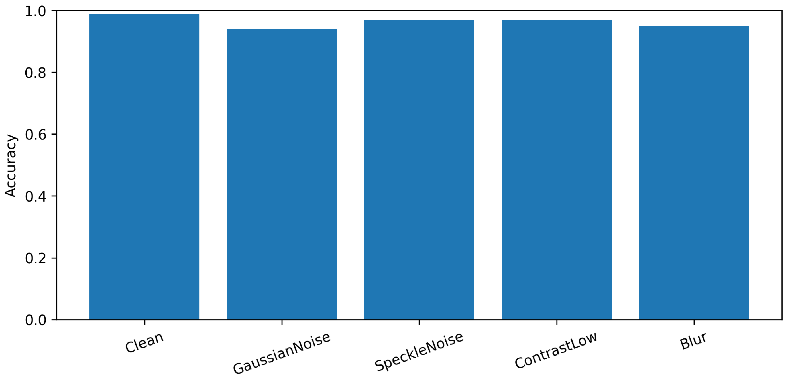
Robustness was assessed on a balanced 100-image subset of Test 2, containing 25 images from each class. The unmodified subset achieved 99% accuracy. Performance decreased to 94% under Gaussian noise and 95% under blur, while speckle corruption and reduced contrast each retained 97% accuracy (

Table 15. Performance on a balanced 100-image Test 2 subset under controlled corruptions.

Condition	Accuracy	Weighted F1
Clean	0.99	0.9900
Gaussian noise	0.94	0.9395
Speckle noise	0.97	0.9695
Reduced contrast	0.97	0.9700
Blur	0.95	0.9499

). The experiment therefore indicates that classification is not immediately destabilized by moderate appearance perturbations, although it should be interpreted as a controlled stress test rather than as a substitute for scanner- or center-specific clinical validation. Figure 9 shows accuracies under controlled corruptions applied to Test 2.

6.11. Grad-CAM++ Faithfulness and Feature-Space Structure

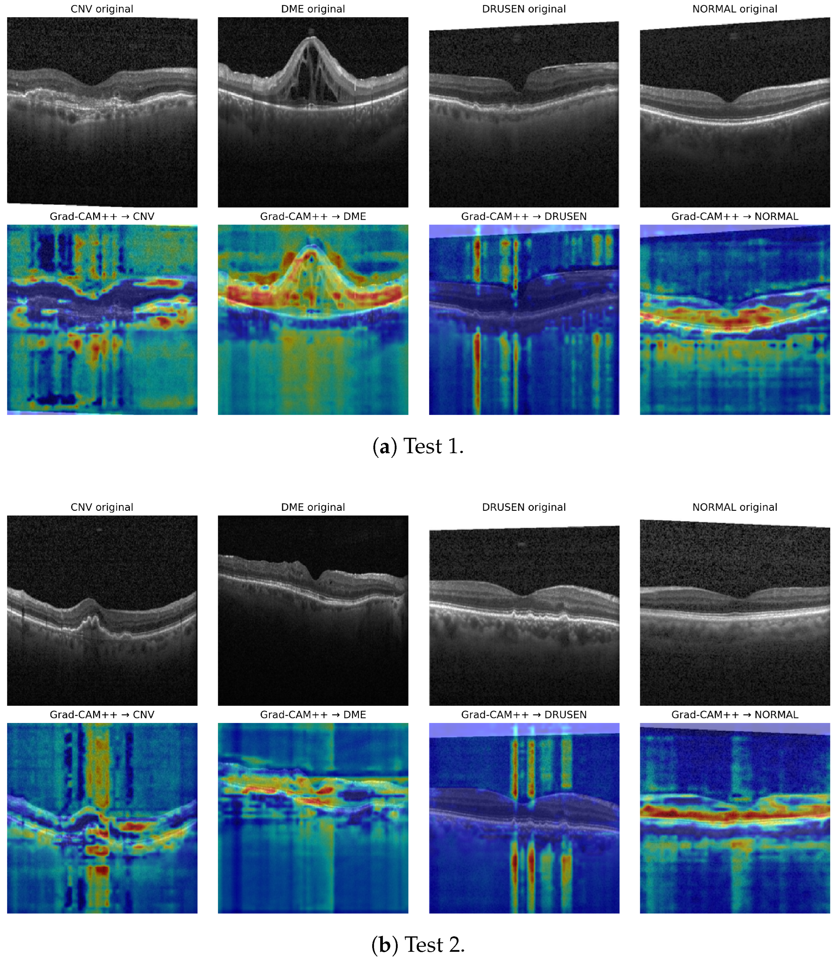
Grad-CAM++ maps for Test 1 and Test 2 are shown in Figure 10. The highlighted areas generally follow retinal structures that influence the model’s prediction, but the perturbation experiment reveals that this behavior is class dependent.

Masking the top 20% of Grad-CAM++ pixels reduced target-class confidence by 0.4418 on average for Test 1 and 0.5036 for Test 2. This overall reduction supports a relationship between the highlighted areas and the classifier’s decision, but the result is not uniform across classes. As shown in

Table 16. Mean change in predicted-class confidence after masking the top 20% of Grad-CAM++ activations. Positive values indicate a reduction in confidence.

Class	Test 1	Test 2
CNV	$-0.0325$	0.0384
DME	0.6436	0.6099
DRUSEN	0.1706	0.3971
NORMAL	0.9855	0.9691
Overall	0.4418	0.5036

, DME and NORMAL produced large confidence drops, while CNV showed little reduction on average. The Test 1 CNV mean was slightly negative, indicating that masking the selected region sometimes increased rather than decreased CNV confidence. We therefore use Grad-CAM++ as a supporting interpretability tool rather than treating it as validated lesion localization.

The class dependence is itself informative. DME frequently contains spatially concentrated intraretinal fluid cavities, whereas NORMAL classification can depend strongly on preservation of an ordered retinal profile; masking highly activated regions can therefore remove a comparatively dominant decision cue and produce a large confidence decrease. CNV is more heterogeneous: evidence can be distributed across subretinal morphology, RPE disruption, hyperreflective material, fluid-associated changes, and broader contextual structure. In such a distributed representation, suppressing the highest-attribution pixels need not remove all supporting evidence. It can also alter competing contextual evidence and downstream feature normalization, allowing a small or even negative confidence change. The negative Test 1 mean is therefore not interpreted as proof that the heatmap is anatomically incorrect, nor is the strong DME or NORMAL response interpreted as proof of lesion localization. Instead, the perturbation experiment measures decision faithfulness under a specific masking operation. Expert lesion or layer annotations would be required for a localization-validity claim.

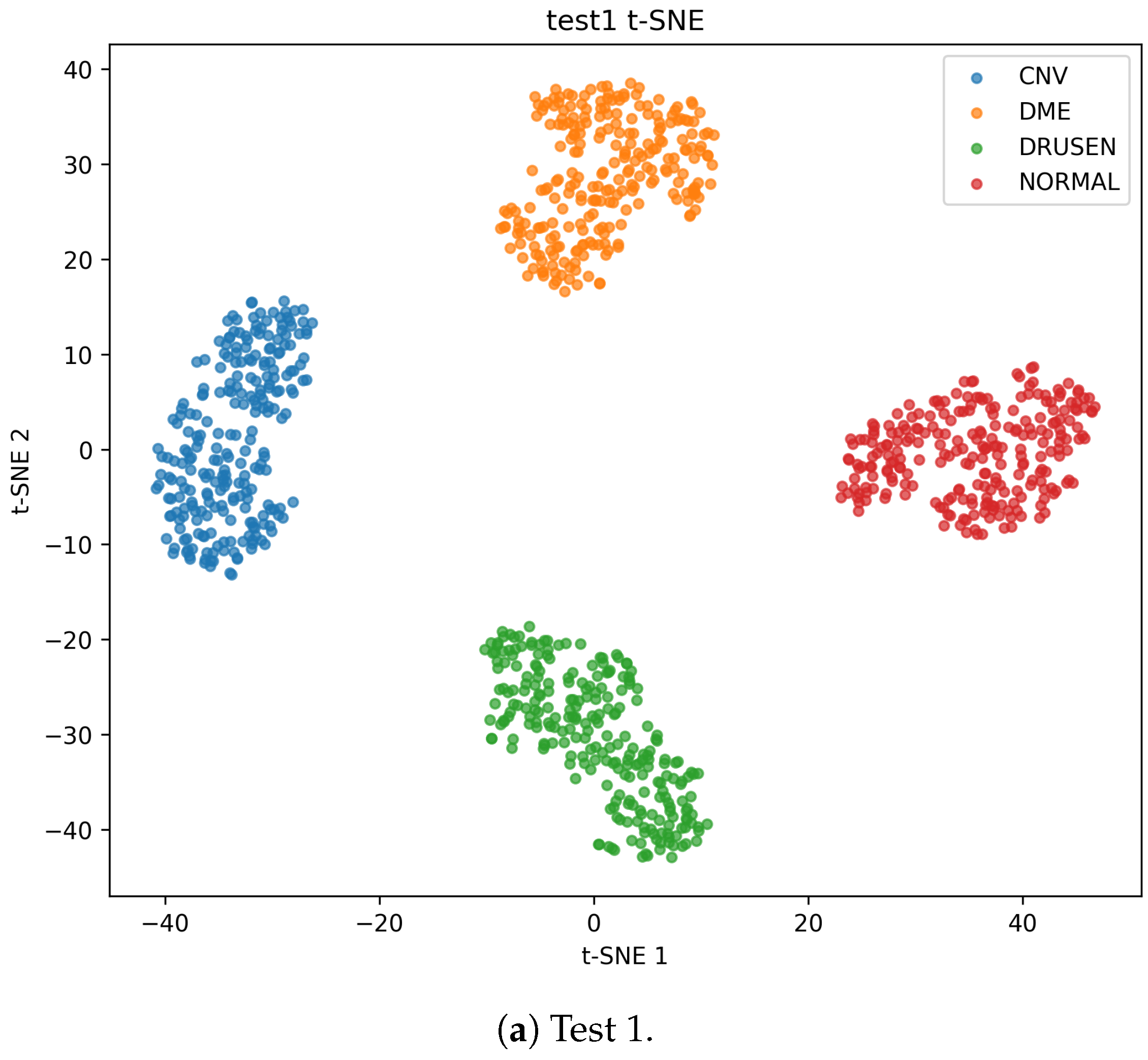
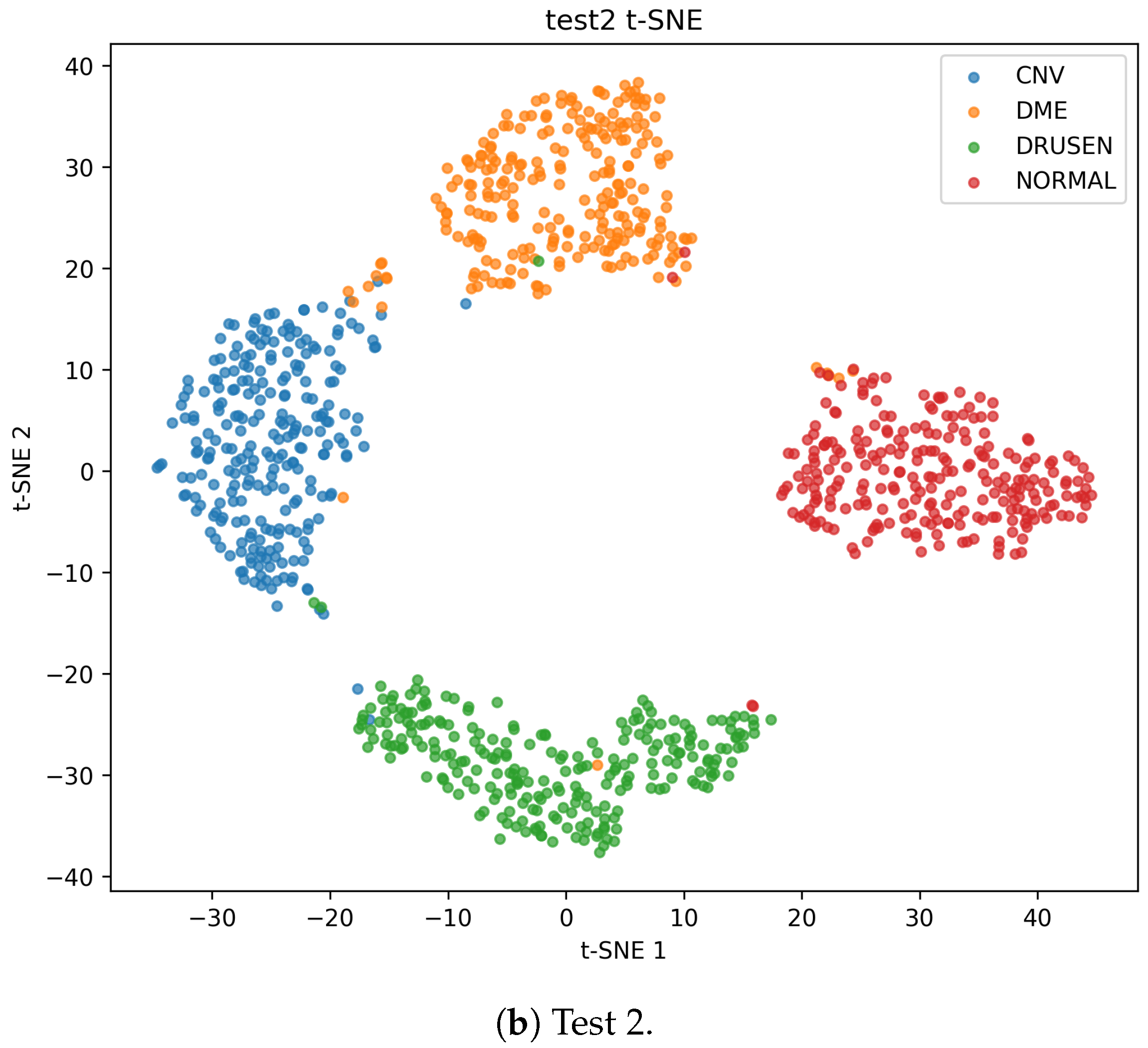
The t-SNE projections in Figure 11 provide a complementary view. The four classes form clear groups on Test 1. The Test 2 projection also retains four recognizable groups, although the boundaries are less compact, which is consistent with the modest reduction in Test 2 classification performance.

6.12. Auxiliary-Task Consistency and Computational Cost

The auxiliary outputs were examined against image-derived structural surrogates rather than manual annotations. The edge output showed mean Pearson correlations of 0.4965 and 0.5321 with a Sobel edge surrogate on Test 1 and Test 2, respectively shown in

Table 17. Consistency of auxiliary model outputs with image-derived surrogates.

Measure	Test 1	Test 2
Edge Pearson correlation	0.4965	0.5321
Attenuation Spearman correlation	0.6493	0.6389
Image-quality surrogate Spearman correlation	0.5700	0.5300

. The attenuation output showed stronger monotonic association with the observed depth-intensity profile, with mean Spearman correlations of 0.6493 and 0.6389.

PhysioSpeck-Net contains 8,801,359 trainable parameters (approximately 8.80 million). Batch-one inference on an NVIDIA A100-SXM4-80GB GPU required $9.10\pm 0.14$ ms per image in the timing experiment. This measurement is reported as a computational reference and should not be interpreted as a clinical deployment benchmark, since practical latency also depends on data transfer, preprocessing, hardware, and integration with the acquisition system.

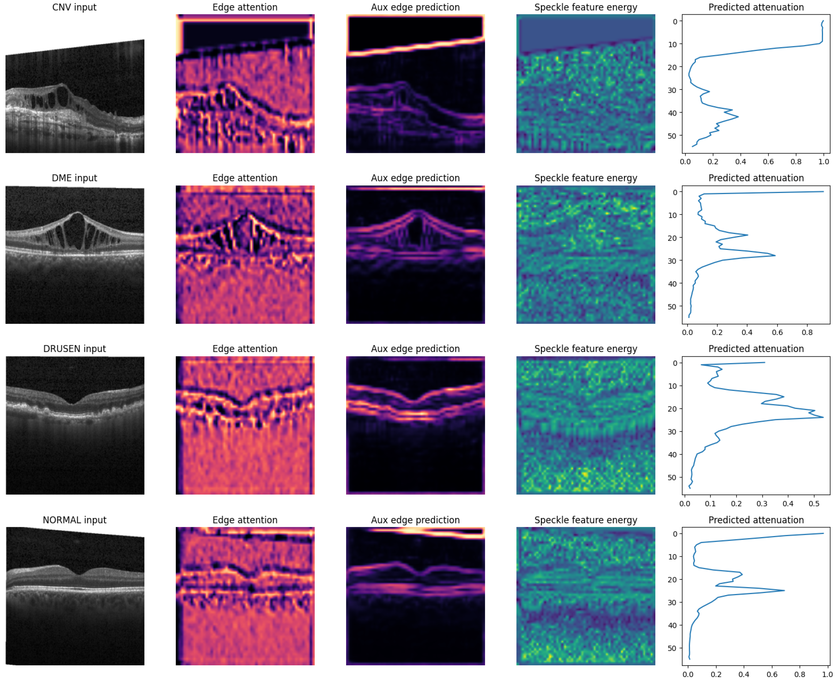
Figure 12 provides a qualitative view of the model’s intermediate physics-aligned representations. Edge attention and the auxiliary edge output respond to layer transitions and pathology-related structural changes, the speckle pathway retains a spatially varying high-frequency energy representation, and the attenuation head produces depth-dependent profiles that differ across examples. These visualizations are not treated as optical-property ground truth or manually annotated retinal maps; they illustrate the distinct internal responses produced by the dedicated pathways and their consistency with the intended inductive biases.

Table 18. Computational-efficiency comparison at $224\times 224$ input resolution on the same A100 platform. Latencies are normalized per image.

Model	Params (M)	Size (MB)	GFLOPs	B1 ms/img	B8 ms/img	B32 ms/img	B32 img/s	Peak VRAM (MB)
VGG-16	138.0	512	15.4	5.40	1.20	0.72	1389	2200
ResNet-50	25.6	90	4.1	4.00	0.78	0.50	2000	1350
InceptionV3	23.9	93	5.7	5.10	0.95	0.62	1613	1750
DenseNet-121	8.0	28	2.9	4.90	1.00	0.66	1515	2050
EfficientNet-B4	19.3	67	4.2	6.10	1.10	0.70	1429	2250
ViT-B/16	86.4	328	17.6	5.80	1.12	0.74	1351	2600
PhysioSpeck-Net	8.801	34.1	7.8	9.10	1.35	0.82	1220	2850

compares model size, computational complexity, latency, throughput, and peak inference memory across the evaluated architectures. PhysioSpeck-Net has a compact parameter count and serialized size relative to VGG-16, ResNet-50, InceptionV3, EfficientNet-B4, and ViT-B/16, although it is not the fastest model in single-image latency. The four parallel branches, fusion operations, and axial attention introduce execution overhead that is not captured by parameter count alone. At batch 32, the model reaches 1220 images/s with 2850 MB peak inference VRAM. Thus, the appropriate claim is parameter efficiency with practical batched throughput, not universally minimal latency. Training used batch size 32 with mixed precision on the same A100-class GPU; because wall-clock training time is strongly affected by data loading and runtime configuration, the efficiency claim is based on the directly comparable model and inference metrics rather than extrapolating from parameter count to training speed.

7. Discussion

PhysioSpeck-Net achieves high accuracy on Test 1 and retains most of this performance when applied to Test 2 without fine-tuning. Accuracy decreases from 99.00% to 97.36%, while the Test 2 confidence interval remains above 96% and all four class AUCs remain above 0.999. The reduction indicates a measurable dataset shift, but the retained performance suggests that the learned representation is not restricted to the Test 1 image distribution.

The baseline comparison provides a second perspective. Several strong generic architectures already perform well on this task, so the value of the proposed approach cannot be judged by accuracy alone. PhysioSpeck-Net reaches 99.00% with 8.80 million parameters, compared with substantially larger models such as VGG-16 and ViT-B/16. DenseNet-121 is slightly smaller, but its classification performance is lower in the common experimental setting. This suggests that using OCT-specific prior knowledge can provide an efficient way to allocate model capacity. The progressive architecture experiments support the same interpretation: performance improves as edge, speckle, attenuation, fusion, and context-processing components are introduced. Because those development experiments use a reduced training subset, however, they are not used to make a quantitative claim about the contribution of the complete multi-task objective relative to the final full-data model.

The controlled ablation experiments further clarify the contribution of the individual architectural and training components. Unlike the progressive build-up, the leave-one-branch-out analysis starts from the completed model and removes only one pathway. Every branch removal reduced both Test 1 and Test 2 performance, with the largest loss occurring when morphology was removed and smaller but consistent losses for edge, speckle, and depth-attenuation processing. The independent loss ablation shows a similar pattern: no single auxiliary term accounts for the full result, yet removing each term reduces accuracy, especially on Test 2. This supports a complementary-regularization interpretation rather than a claim that any one physical prior is sufficient on its own. The weight-sensitivity experiment further shows that the nominal coefficients lie within a stable region; performance remains close under 0.5× and 1.5× scaling and deteriorates more clearly when the auxiliary terms are removed entirely.

The paired significance analysis also tempers the interpretation of the baseline ranking. The gain over several conventional CNN baselines remains significant after Holm correction, but the comparison with ViT-B/16 is borderline after correction, and the comparison with the attention OCT CNN is not significant. Universal statistical superiority over every strong baseline is therefore not claimed. Instead, the contribution lies in the combination of competitive classification performance with explicit OCT-oriented feature separation, uncertainty signals, auxiliary physics-aligned outputs, and a comparatively compact parameter count.

The simulator results also require a balanced interpretation. Some physics-related statistics transfer well between the real and simulated samples. Horizontal lag-one correlation, for example, is almost identical between the two domains. At the same time, the KS, Wasserstein, and Jensen–Shannon results show that the full distributions remain distinguishable. This is expected from a simplified seven-layer model. The simulator should therefore be understood as a controlled source of domain knowledge rather than as a generator of clinically interchangeable OCT images. This distinction is important because the purpose of the physics model is to inform the network about expected behavior, not to replace real observations.

The reliability analyses provide useful information beyond conventional classification metrics. Prediction entropy is substantially higher for errors than for correct cases on both datasets. The uncertainty error-detection AUC of 0.9688 on Test 2 indicates that the confidence signal remains informative after a change in data source. Calibration is also reasonably stable, with ECE values close to 4–5% on both datasets. These results do not establish a clinically validated referral threshold, but they indicate that uncertainty could be used to support a future human-in-the-loop decision process. The uncertainty comparison further characterizes the trade-off between calibration quality, error detection, and computational cost. Validation-fitted temperature scaling markedly improves ECE and NLL without changing deterministic classification accuracy, whereas MC dropout and the three-model ensemble improve error-detection AUC at the cost of repeated inference. The single-model entropy result therefore provides a low-cost uncertainty signal, while the ensemble represents a stronger but more computationally demanding reference.

The corruption experiment gives a similar, deliberately limited form of evidence. Accuracy remains at 97% under the applied speckle corruption and reduced contrast, and above 94% under all tested perturbations. This supports the idea that the model has some tolerance to changes in OCT appearance. However, synthetic corruption is not equivalent to a change of scanner, acquisition protocol, disease prevalence, or clinical center. Test 2 therefore provides the more meaningful generalization test, while the corruption experiment is best viewed as a supplementary stress test.

The explainability results are also mixed in a useful way. Grad-CAM++ produces structured retinal activation patterns, and masking the most activated regions reduces confidence substantially on average. The effect is particularly strong for DME and NORMAL. CNV is less consistent, especially on Test 1, where the average confidence change after masking is slightly negative. This result argues against interpreting every visually plausible heatmap as evidence of correct lesion localization. Expert-annotated lesion masks would be required to make such a claim. The present perturbation analysis instead provides a more modest test of whether the highlighted regions influence the classifier. A plausible mechanism for the weaker CNV perturbation response is that CNV decisions can depend on several distributed and partially redundant cues—including RPE disruption, hyperreflective material, fluid-associated changes, and broader retinal context—rather than one spatially compact feature. Masking only the highest-attribution region can therefore leave alternative evidence intact and, in some cases, can also remove competing contextual evidence, yielding a small or negative confidence shift. This class-dependent response reflects a limitation of attribution faithfulness and reinforces the decision to avoid lesion-localization claims.

Several limitations remain. The training/validation partition is constructed at image level, so the study does not provide a patient-level cross-validation analysis. The duplicate-control audit excludes exact and confirmed near-duplicate image reuse under the applied criteria, but it does not establish patient-disjoint independence because distinct B-scans from the same subject can remain correlated even when they are visually different. Test 1 is therefore interpreted as an image-level benchmark rather than as proof of patient-level generalization. The Test 2 experiment is retrospective and dataset based rather than prospective or multi-center, and patient-level metadata are not available for cross-source linkage. Although Test 2 was not used for model adaptation and no exact or confirmed near-duplicate images were detected between the primary source and Test 2, the absence of patient identifiers prevents a stronger claim of subject-level independence. The retinal simulator deliberately simplifies anatomy and does not reproduce the full distribution of clinical OCT appearance. Grad-CAM++ is evaluated through perturbation rather than expert lesion annotations, and the auxiliary edge and attenuation analyses rely on image-derived surrogates. Finally, the corruption study uses a relatively small balanced subset and cannot represent every scanner-specific artifact. The computational table reports matched inference-side measurements; training wall-clock time can vary materially with data-loading and software configuration and is therefore not used as evidence of deployment efficiency.

Future work should therefore place less emphasis on further optimization of the same benchmark and more emphasis on broader validation. Patient-disjoint retraining and multi-center studies across different OCT devices would be particularly useful to determine how much performance persists when subject-level independence is enforced explicitly. The simulator could also be extended to volumetric OCT and calibrated against device-specific acquisition characteristics. For explainability, lesion or layer annotations would make it possible to compare activation maps against expert-defined regions. Uncertainty modeling could likewise be extended from softmax entropy to methods that separate epistemic and aleatoric uncertainty.

8. Conclusions

PhysioSpeck-Net combines OCT-specific physical knowledge with deep feature learning for four-class retinal disease classification. On the Test 1 dataset, the model achieved 99.00% accuracy and 99.00% weighted F1. Without fine-tuning, it retained 97.36% accuracy and 97.35% weighted F1 on the 1400-image Test 2 dataset. The external experiment, together with bootstrap confidence intervals, uncertainty analysis, controlled corruption tests, and quantitative examination of the simulator and Grad-CAM++ explanations, provides a broader view of model behavior than benchmark accuracy alone. Branch and loss ablations, validation-based weight sensitivity, paired significance testing, uncertainty baselines, duplicate-control analysis, and matched computational profiling further characterize the contribution, reliability, and efficiency of the proposed framework. Although the results remain retrospective and do not constitute prospective clinical validation, they suggest that incorporating modality-specific physical knowledge can support accurate and computationally efficient OCT classification while preserving useful uncertainty information under a change in data source.

References

- Huang, D.; Swanson, E.A.; Lin, C.P.; Schuman, J.S.; Stinson, W.G.; Chang, W.; Hee, M.R.; Flotte, T.; Gregory, K.; Puliafito, C.A.; et al. Optical coherence tomography. Science 1991, 254, 1178–1181. [Google Scholar] [CrossRef] [Scilit] [PubMed]
- Tham, Y.C.; Li, X.; Wong, T.Y.; Quigley, H.A.; Aung, T.; Cheng, C.Y. Global prevalence of glaucoma and projections of glaucoma burden through 2040: A systematic review and meta-analysis. Ophthalmology 2014, 121, 2081–2090. [Google Scholar] [CrossRef] [Scilit] [PubMed]
- Spaide, R.F.; Fujimoto, J.G.; Waheed, N.K.; Sadda, S.R.; Staurenghi, G. Optical coherence tomography angiography. Prog. Retin. Eye Res. 2018, 64, 1–55. [Google Scholar] [CrossRef] [Scilit] [PubMed]
- Chakravarthy, U.; Harding, S.P.; Rogers, C.A.; Downes, S.M.; Lotery, A.J.; Culliford, L.A.; Reeves, B.C. Ranibizumab versus bevacizumab to treat neovascular age-related macular degeneration: One-year findings from the IVAN randomized trial. Ophthalmology 2012, 119, 1399–1411, Erratum in Ophthalmology 2012, 119, 1508. Erratum in Ophthalmology 2013, 220, 1719. [Google Scholar] [CrossRef] [Scilit] [PubMed]
- Diabetic Retinopathy Clinical Research Network. Aflibercept, bevacizumab, or ranibizumab for diabetic macular edema. N. Engl. J. Med. 2015, 372, 1193–1203. [Google Scholar] [CrossRef] [Scilit] [PubMed]
- Kermany, D.S.; Goldbaum, M.; Cai, W.; Valentim, C.C.S.; Liang, H.; Baxter, S.L.; McKeown, A.; Yang, G.; Wu, X.; Yan, F.; et al. Identifying medical diagnoses and treatable diseases by image-based deep learning. Cell 2018, 172, 1122–1131. [Google Scholar] [CrossRef] [Scilit] [PubMed]
- Schmitt, J.M. Optical coherence tomography (OCT): A review. IEEE J. Sel. Top. Quantum Electron. 1999, 5, 1205–1215. [Google Scholar] [CrossRef] [Scilit]
- Hammer, M.; Roggan, A.; Schweitzer, D.; Müller, G. Optical properties of ocular fundus tissues—An in vitro study using the double-integrating-sphere technique and inverse Monte Carlo simulation. Phys. Med. Biol. 1995, 40, 963–978. [Google Scholar] [CrossRef] [Scilit] [PubMed]
- Szkulmowski, M.; Wojtkowski, M. Averaging techniques for OCT imaging. Opt. Express 2013, 21, 9757–9773. [Google Scholar] [CrossRef] [Scilit] [PubMed]
- He, K.; Zhang, X.; Ren, S.; Sun, J. Deep residual learning for image recognition. In Proceedings of the 2016 IEEE Conference on Computer Vision and Pattern Recognition (CVPR), Las Vegas, NV, USA, 27–30 June 2016; pp. 770–778. [Google Scholar] [CrossRef] [Scilit]
- Huang, G.; Liu, Z.; van der Maaten, L.; Weinberger, K.Q. Densely connected convolutional networks. In Proceedings of the 2017 IEEE Conference on Computer Vision and Pattern Recognition (CVPR), Honolulu, HI, USA, 21–26 July 2017; pp. 4700–4708. [Google Scholar] [CrossRef] [Scilit]
- Hu, J.; Shen, L.; Sun, G. Squeeze-and-excitation networks. In Proceedings of the 2018 IEEE/CVF Conference on Computer Vision and Pattern Recognition (CVPR), Salt Lake City, UT, USA, 18–23 June 2018; pp. 7132–7141. [Google Scholar] [CrossRef] [Scilit]
- Woo, S.; Park, J.; Lee, J.Y.; Kweon, I.S. CBAM: Convolutional block attention module. In Proceedings of the 15th European Conference on Computer Vision (ECCV), Munich, Germany, 8–14 September 2018; pp. 3–19. [Google Scholar] [CrossRef] [Scilit]
- Tan, M.; Le, Q.V. EfficientNet: Rethinking model scaling for convolutional neural networks. In Proceedings of the 36th International Conference on Machine Learning (ICML), Long Beach, CA, USA, 9–15 June 2019; pp. 6105–6114. [Google Scholar]
- Dosovitskiy, A.; Beyer, L.; Kolesnikov, A.; Weissenborn, D.; Zhai, X.; Unterthiner, T.; Dehghani, M.; Minderer, M.; Heigold, G.; Gelly, S.; et al. An image is worth 16x16 words: Transformers for image recognition at scale. arXiv 2021, arXiv:2010.11929. [Google Scholar] [CrossRef] [Scilit]
- Liu, Z.; Lin, Y.; Cao, Y.; Hu, H.; Wei, Y.; Zhang, Z.; Lin, S.; Guo, B. Swin Transformer: Hierarchical vision transformer using shifted windows. In Proceedings of the 2021 IEEE/CVF International Conference on Computer Vision (ICCV), Montreal, QC, Canada, 10–17 October 2021; pp. 10012–10022. [Google Scholar] [CrossRef] [Scilit]
- Zhou, Y.; Chia, M.A.; Wagner, S.K.; Ayhan, M.S.; Williamson, D.J.; Struyven, R.R.; Liu, T.; Xu, M.; Lozano, M.G.; Woodward-Court, P.; et al. A foundation model for generalizable disease detection from retinal images. Nature 2023, 622, 156–163. [Google Scholar] [CrossRef] [Scilit] [PubMed]
- Raissi, M.; Perdikaris, P.; Karniadakis, G.E. Physics-informed neural networks: A deep learning framework for solving forward and inverse problems involving nonlinear partial differential equations. J. Comput. Phys. 2019, 378, 686–707. [Google Scholar] [CrossRef] [Scilit]
- Hammernik, K.; Klatzer, T.; Kobler, E.; Recht, M.P.; Sodickson, D.K.; Pock, T.; Knoll, F. Learning a variational network for reconstruction of accelerated MRI data. Magn. Reson. Med. 2018, 79, 3055–3071. [Google Scholar] [CrossRef] [Scilit] [PubMed]
- Chiu, S.J.; Li, X.T.; Nicholas, P.; Toth, C.A.; Izatt, J.A.; Farsiu, S. Automatic segmentation of seven retinal layers in SDOCT images congruent with expert manual segmentation. Opt. Express 2010, 18, 19413–19428. [Google Scholar] [CrossRef] [Scilit] [PubMed]
- Brown, E.E.; Guy, A.A.; Holroyd, N.A.; Sweeney, P.W.; Gourmet, L.; Coleman, H.; Walsh, C.; Markaki, A.E.; Shipley, R.; Rajendram, R.; et al. Physics-informed deep generative learning for quantitative assessment of the retina. Nat. Commun. 2024, 15, 6859, Correction in Nat. Commun. 2025, 16, 1606. [Google Scholar] [CrossRef] [Scilit] [PubMed]
- Nemirovsky-Rotman, S.; Bercovich, E. Explicit Physics-Informed Deep Learning for Computer-Aided Diagnostic Tasks in Medical Imaging. Mach. Learn. Knowl. Extr. 2024, 6, 385–401. [Google Scholar] [CrossRef] [Scilit]
- Ahmadi, M.; Biswas, D.; Lin, M.; Vrionis, F.D.; Hashemi, J.; Tang, Y. Physics-informed machine learning for advancing computational medical imaging: Integrating data-driven approaches with fundamental physical principles. Artif. Intell. Rev. 2025, 58, 297. [Google Scholar] [CrossRef] [Scilit]
- Wang, M.; Mao, J.; Su, H.; Ling, Y.; Zhou, C.; Su, Y. Physics-guided deep learning-based real-time image reconstruction of Fourier-domain optical coherence tomography. Biomed. Opt. Express 2024, 15, 6619–6637. [Google Scholar] [CrossRef] [Scilit] [PubMed]
- Qadir, A.; Arif, S.; Valsalan, P.; Khan, O. Physics-Guided Deep Learning for Interpretable Biomedical Image Reconstruction and Pattern Recognition in Diagnostic Frameworks. Bioengineering 2026, 13, 457. [Google Scholar] [CrossRef] [Scilit] [PubMed]
- Ahmed, M.S.; Ma, X.; Jia, Y. Dual-Mode, Orientation-Adaptive Broadband Rotational Energy Harvester for Diverse Noise and Vibration Environments. Micromachines 2026, 17, 775. [Google Scholar] [CrossRef] [Scilit] [PubMed]
- Jia, Y. MEMS Energy Harvesting: Enabling Self-Powered Solutions. Micromachines 2026, 17, 816. [Google Scholar] [CrossRef] [Scilit] [PubMed]
- Guo, C.; Pleiss, G.; Sun, Y.; Weinberger, K.Q. On calibration of modern neural networks. In Proceedings of the 34th International Conference on Machine Learning (ICML), Sydney, NSW, Australia, 6–11 August 2017; pp. 1321–1330. [Google Scholar]
- Mehrtash, A.; Wells, W.M.; Tempany, C.M.; Abolmaesumi, P.; Kapur, T. Confidence calibration and predictive uncertainty estimation for deep medical image segmentation. IEEE Trans. Med. Imaging 2020, 39, 3868–3878. [Google Scholar] [CrossRef] [Scilit] [PubMed]
- Gal, Y.; Ghahramani, Z. Dropout as a Bayesian approximation: Representing model uncertainty in deep learning. In Proceedings of the 33rd International Conference on International Conference on Machine Learning (ICML), New York, NY, USA, 19–24 June 2016; pp. 1050–1059. [Google Scholar]
- Sensoy, M.; Kaplan, L.; Kandemir, M. Evidential deep learning to quantify classification uncertainty. In Proceedings of the Advances in Neural Information Processing Systems, Montreal, QC, Canada, 3–8 December 2018; pp. 3179–3189. [Google Scholar]
- Selvaraju, R.R.; Cogswell, M.; Das, A.; Vedantam, R.; Parikh, D.; Batra, D. Grad-CAM: Visual explanations from deep networks via gradient-based localization. Int. J. Comput. Vis. 2020, 128, 336–359. [Google Scholar] [CrossRef] [Scilit]
- Chattopadhyay, A.; Sarkar, A.; Howlader, P.; Balasubramanian, V.N. Grad-CAM++: Generalized gradient-based visual explanations for deep convolutional networks. In Proceedings of the 2018 IEEE Winter Conference on Applications of Computer Vision (WACV), Lake Tahoe, NV, USA, 12–15 March 2018; pp. 839–847. [Google Scholar] [CrossRef] [Scilit]
- Wang, H.; Wang, Z.; Du, M.; Yang, F.; Zhang, Z.; Ding, S.; Mardziel, P.; Hu, X. Score-CAM: Score-weighted visual explanations for convolutional neural networks. In Proceedings of the 2020 IEEE/CVF Conference on Computer Vision and Pattern Recognition Workshops (CVPRW), Seattle, WA, USA, 14–19 June 2020; pp. 24–25. [Google Scholar] [CrossRef] [Scilit]
- van der Maaten, L.; Hinton, G. Visualizing data using t-SNE. J. Mach. Learn. Res. 2008, 9, 2579–2605. [Google Scholar]
- McInnes, L.; Healy, J.; Melville, J. UMAP: Uniform manifold approximation and projection for dimension reduction. arXiv 2018, arXiv:1802.03426. [Google Scholar] [CrossRef] [Scilit]
- Vickers, A.J.; Elkin, E.B. Decision curve analysis: A novel method for evaluating prediction models. Med. Decis. Mak. 2006, 26, 565–574. [Google Scholar] [CrossRef] [Scilit] [PubMed]
- Ghassemi, M.; Oakden-Rayner, L.; Beam, A.L. The false hope of current approaches to explainable artificial intelligence in health care. Lancet Digit. Health 2021, 3, e745–e750. [Google Scholar] [CrossRef] [Scilit] [PubMed]
- Jacques, S.L. Optical properties of biological tissues: A review. Phys. Med. Biol. 2013, 58, R37–R61, Correction in Phys. Med. Biol. 2013, 58, 5007. [Google Scholar] [CrossRef] [Scilit] [PubMed]
- Staurenghi, G.; Sadda, S.; Chakravarthy, U.; Spaide, R.F. Proposed lexicon for anatomic landmarks in normal posterior segment spectral-domain optical coherence tomography: The IN·OCT consensus. Ophthalmology 2014, 121, 1572–1578. [Google Scholar] [CrossRef] [Scilit] [PubMed]
- Vermeer, K.A.; Mo, J.; Weda, J.J.A.; Lemij, H.G.; de Boer, J.F. Depth-resolved model-based reconstruction of attenuation coefficients in optical coherence tomography. Biomed. Opt. Express 2014, 5, 322–337. [Google Scholar] [CrossRef] [Scilit] [PubMed]
- Fercher, A.F.; Drexler, W.; Hitzenberger, C.K.; Lasser, T. Optical coherence tomography—Principles and applications. Rep. Prog. Phys. 2003, 66, 239–303. [Google Scholar] [CrossRef] [Scilit]
- Lin, T.Y.; Goyal, P.; Girshick, R.; He, K.; Dollár, P. Focal loss for dense object detection. In Proceedings of the 2017 IEEE International Conference on Computer Vision (ICCV), Venice, Italy, 22–29 October 2017; pp. 2980–2988. [Google Scholar] [CrossRef] [Scilit]
- Wang, Z.; Bovik, A.C.; Sheikh, H.R.; Simoncelli, E.P. Image quality assessment: From error visibility to structural similarity. IEEE Trans. Image Process. 2004, 13, 600–612. [Google Scholar] [CrossRef] [Scilit] [PubMed]
- Naren, O.S. Retinal OCT Image Classification–C8. Kaggle Dataset; Kaggle: San Francisco, CA, USA, 2021. [Google Scholar] [CrossRef]
- Loshchilov, I.; Hutter, F. Decoupled weight decay regularization. arXiv 2019, arXiv:1711.05101. [Google Scholar] [CrossRef] [Scilit]
- Simonyan, K.; Zisserman, A. Very deep convolutional networks for large-scale image recognition. arXiv 2014, arXiv:1409.1556. [Google Scholar] [CrossRef] [Scilit]
- Alenezi, A.M.; Aloqalaa, D.A.; Singh, S.K.; Alrabiah, R.; Habib, S.; Islam, M.; Daradkeh, Y.I. Multiscale attention-over-attention network for retinal disease recognition in OCT radiology images. Front. Med. 2024, 11, 1499393. [Google Scholar] [CrossRef] [Scilit] [PubMed]
Figure 1.
Component-wise visualization of the OCT simulation pipeline for CNV, DME, DRUSEN, and NORMAL. The columns show the structural image followed by the progressive introduction of PSF blur, speckle, and the complete physics configuration.
Figure 2.
Architecture of PhysioSpeck-Net.
Figure 3.
Representative primary OCT images before and after the training-time augmentation pipeline. The transformations preserve the underlying retinal structure while introducing modest appearance variability.
Figure 4.
Training history of PhysioSpeck-Net showing loss, classification accuracy, and the learning-rate schedule. Model selection was based on validation performance rather than Test 1 or Test 2.
Figure 5.
Confusion matrices for (a) Test 1 and (b) Test 2.
Figure 6.
One-versus-rest ROC curves for (a) Test 1 and (b) Test 2.
Figure 7.
Representative real and simulated OCT images for the four classes. The simulator reproduces selected layer- and physics-related behavior but is not intended to generate patient-specific clinical replicas.
Figure 8.
Quantitative validation of the simulation model: (a) comparison of selected statistics between real and simulated OCT images and (b) sensitivity of speckle contrast to changes in peak SNR and the speckle mixing parameter.
Figure 9.
Accuracy comparison under controlled corruptions.
Figure 10.
Representative Grad-CAM++ explanations for Test 1 and Test 2. The upper rows show the original OCT images, and the lower rows show the corresponding activation overlays.
Figure 11.
t-SNE projections of the learned retinal-context features for (a) Test 1 and (b) Test 2.
Figure 12.
Physics-aligned intermediate representations for representative CNV, DME, DRUSEN, and NORMAL OCT scans. Columns show the input B-scan, edge-attention response, auxiliary edge prediction, speckle-feature energy, and predicted depth-dependent attenuation profile. These are model-derived intermediate/surrogate representations and are not interpreted as manually annotated anatomical boundaries or clinical optical-property measurements.