Toward Clinically Trustworthy Pathology Foundation Models for Microsatellite Instability Prescreening in Colorectal Cancer

Abstract

Pathology foundation models have recently emerged as powerful pretrained representations for computational pathology, yet whether complex downstream modeling is still necessary once frozen representations are evaluated under a common downstream framework remains insufficiently understood. We address this question for microsatellite-instability-high (MSI-H) prediction in colorectal cancer by benchmarking nine frozen encoders—five pathology-specific (CONCH, CONCH v1.5, UNI, Virchow2, Phikon) and four conventional vision backbones (ResNet18, ResNet50, ViT-B/16, ConvNeXt-Tiny)—for colorectal cancer histopathology under a patient-level framework, using TCGA-COAD/READ as the development cohort and CPTAC-COAD as an independent external cohort. For each encoder, H&E tiles were embedded without fine-tuning, mean-pooled to slide and patient representations, and evaluated with the same logistic regression linear probe, alongside nonlinear classifiers and a gated-attention multiple-instance learning (MIL) comparator. The complete MANTIS-defined 206-patient cohort (82 MSI-H, 124 MSS) is reported as the primary development benchmark. A label provenance audit identified 15 of 206 development cohort patients (7.3%) with cross-source MSI provenance discordance, and the concordant-label 191-patient cohort (68 MSI-H, 123 MSS) is reported as a secondary sensitivity analysis. In the primary cohort, the selected pathology-specific encoders had a higher mean pooled out-of-fold AUROC than the selected conventional vision backbones (0.827 vs. 0.773; paired-bootstrap difference, +0.054; 95% interval, +0.015 to +0.094), which is reported as a descriptive benchmark rather than a formal inference about the model classes. Virchow2 and UNI produced the strongest linear probe discrimination (AUROC 0.861 and 0.855, respectively), with no consistent gain from the tested nonlinear classifiers or attention–MIL configurations, and representational similarity analysis (linear centered kernel alignment) confirmed that encoders occupy distinct feature geometries rather than converging to a shared representation. In external validation on CPTAC-COAD (105 patients; 24 MSI-H, 81 MSS), selected TCGA-trained models retained variable discrimination, including CONCH attention–MIL AUROC 0.880 and UNI linear probe AUROC 0.859, but external calibration and threshold behavior varied substantially; for CONCH attention–MIL, the development-derived threshold did not transport under the external ensemble implementation (specificity 0.000), whereas threshold-only local adaptation on a small external subset improved median specificity to 0.686 without updating model weights. These findings indicate that modern pathology foundation models can encode MSI-associated morphology in frozen representations under this benchmark, while decision threshold transportability and multimodal or explainability extensions remain open questions for future work.

1. Introduction

Colorectal cancer is one of the major global disease burdens, accounting for 9.6% of newly diagnosed cancer cases and 9.3% of cancer-related deaths worldwide according to GLOBOCAN 2022 [1]. Molecular stratification has become increasingly important for prognosis and treatment selection in this disease [2,3]. In particular, stratification of MSI-H status is especially important because immune checkpoint inhibition has been shown to provide clinical benefit in appropriately selected patients [4,5]. Assessment of MSI (microsatellite instability) status using polymerase chain reaction (PCR) has been widely applied in colorectal cancer screening because it contributes to the evaluation of Lynch syndrome and may provide information for treatment decision making [6,7,8,9]. Although this method is a standard for clinical reference, it requires additional genetic testing or immunohistochemical procedures, time, and technical resources, and MSI testing may not be consistently completed in every eligible patient [3,10,11,12]. Current professional guidance continues to emphasize appropriate MMR/MSI testing for clinical decision making [13]. Therefore, developing computational prescreening strategies based on routinely available hematoxylin- and eosin-stained histopathology slides may reduce these limitations during the initial stage of molecular screening [14,15,16].

Studies have demonstrated that deep learning models can predict MSI status directly from H&E-stained histological slides [15,16,17,18]. Early approaches generally relied on convolutional neural networks trained or fine-tuned for a specific prediction task [15,16,17,18]. In a large international study, deep learning achieved the ability to detect colorectal cancer samples with dMMR or MSI with a mean AUROC of 0.92 and could stratify colorectal cancer at large scale and low cost [15]. Subsequent studies have further investigated automated MSI prediction and its potential use for prescreening or prioritization of molecular testing [14,19,20]. More recently, deep learning models have increasingly been pretrained on larger and more diverse input datasets, such as large collections of unlabeled images or heterogeneous whole-slide images, to learn diverse morphological tissue features [21,22,23,24,25,26,27,28]. Deep learning models such as UNI, CONCH, Virchow, Virchow2, and Phikon differ substantially in pretraining data, objective functions, model scale, and image resolution [21,22,23,29,30], but each aims to provide reusable features for subsequent computational pathology tasks. Representations extracted by frozen image encoders can be used as inputs for downstream linear classifiers, nonlinear machine learning algorithms, or multiple-instance learning models, as increasingly examined in standardized pathology foundation model benchmarks [31,32,33,34,35]. For whole-slide analysis, clustering-constrained attention multiple-instance learning aggregates variable numbers of patch-level feature vectors into slide-level representations and requires only slide-level labels, without pixel-, region-, or patch-level annotations [36,37,38]. Beyond molecular biomarker prediction, deep learning analysis of histopathology has also been investigated for clinically relevant tasks such as prognosis, risk stratification, and treatment response prediction across cancer types [39].

Although deep learning models have been increasingly developed to facilitate MSI screening, several issues remain unresolved. First, pathology-specific foundation models and conventional vision backbones are often evaluated using different cohorts, preprocessing procedures, downstream classifiers, and validation designs, making it difficult to determine whether observed performance differences reflect the quality of the frozen representations or differences in the pipeline [31,32,33,34]. Therefore, a controlled comparison under a common frozen feature framework is needed. Second, it remains uncertain whether subsequently developed, more complex models can improve predictive performance and thereby improve clinical relevance when a strong frozen representation is already available [32,33,34]. Third, preserved discrimination in an external cohort does not necessarily mean that predicted probabilities and decision thresholds are also preserved. Histopathology models can be sensitive to differences in image acquisition, staining, institutional characteristics, and other hidden variables, resulting in a domain shift when applied to new cohorts [40,41,42,43]. Moreover, probability distributions may shift or lose calibration because discrimination and calibration represent distinct dimensions of predictive performance [44,45,46,47]. This indicates that, even when discrimination is preserved during external validation, predicted probabilities or decision thresholds may still be altered when the model is applied to a completely new dataset.

This study aimed to evaluate the performance of nine frozen image encoders for MSI-H prediction from colorectal cancer histopathology while comparing the task utility of their frozen representations under a common downstream framework. We conducted the study with three main objectives: to compare frozen representations generated by pathology-specific foundation models and conventional vision backbones under a common evaluation framework; to determine whether the tested nonlinear classifiers or attention-based multiple-instance learning (MIL) configuration can provide consistent and practically meaningful improvements in MSI-H discrimination compared with a simple linear probe; and to separately assess external discrimination, probability calibration, and the transportability of development-derived decision thresholds. We hypothesized that pathology-pretrained encoders would generate MSI-H-related representations that were sufficiently linearly separable for regularized linear probes to achieve performance comparable to that of the more complex downstream models tested. In addition, we hypothesized that model discrimination, probability calibration, and development-derived decision thresholds would be preserved when the models were applied to an independent external cohort.

2. Materials and Methods

2.1. Study Design

This study was designed as a frozen-representation benchmark rather than as a task-specific model-optimization study. The primary question was whether pathology-specific foundation models provide more discriminative frozen representations for MSI-H prediction than conventional computer-vision backbones under an identical patient-level evaluation framework. The benchmark pipeline was fixed as follows: H&E image tiles were passed through a frozen encoder, tile embeddings were mean-pooled to slide embeddings, slide embeddings were mean-pooled to a patient embedding, and the patient embedding was evaluated with the same logistic regression linear probe to produce a patient-level MSI-H probability. No encoder was fine-tuned at any stage.

The main comparison was defined at the frozen-representation level while acknowledging that the encoders also differ in architecture, scale, embedding dimensionality, input resolution, pretraining objective, and pretraining data. Encoders were divided into pathology-specific models (CONCH, CONCH v1.5, UNI, Virchow2, and Phikon) and conventional vision backbones (ResNet18, ResNet50, ViT-B/16 pretrained on ImageNet-21k, and ConvNeXt-Tiny). The primary endpoint was a pooled out-of-fold AUROC from the linear probe on the development cohort. The secondary analyses assessed nonlinear classifier dependence, attention–MIL performance, representational similarity, calibration, external transportability, local threshold adaptation, and top-tile interpretability artifacts.

2.2. Development Cohort

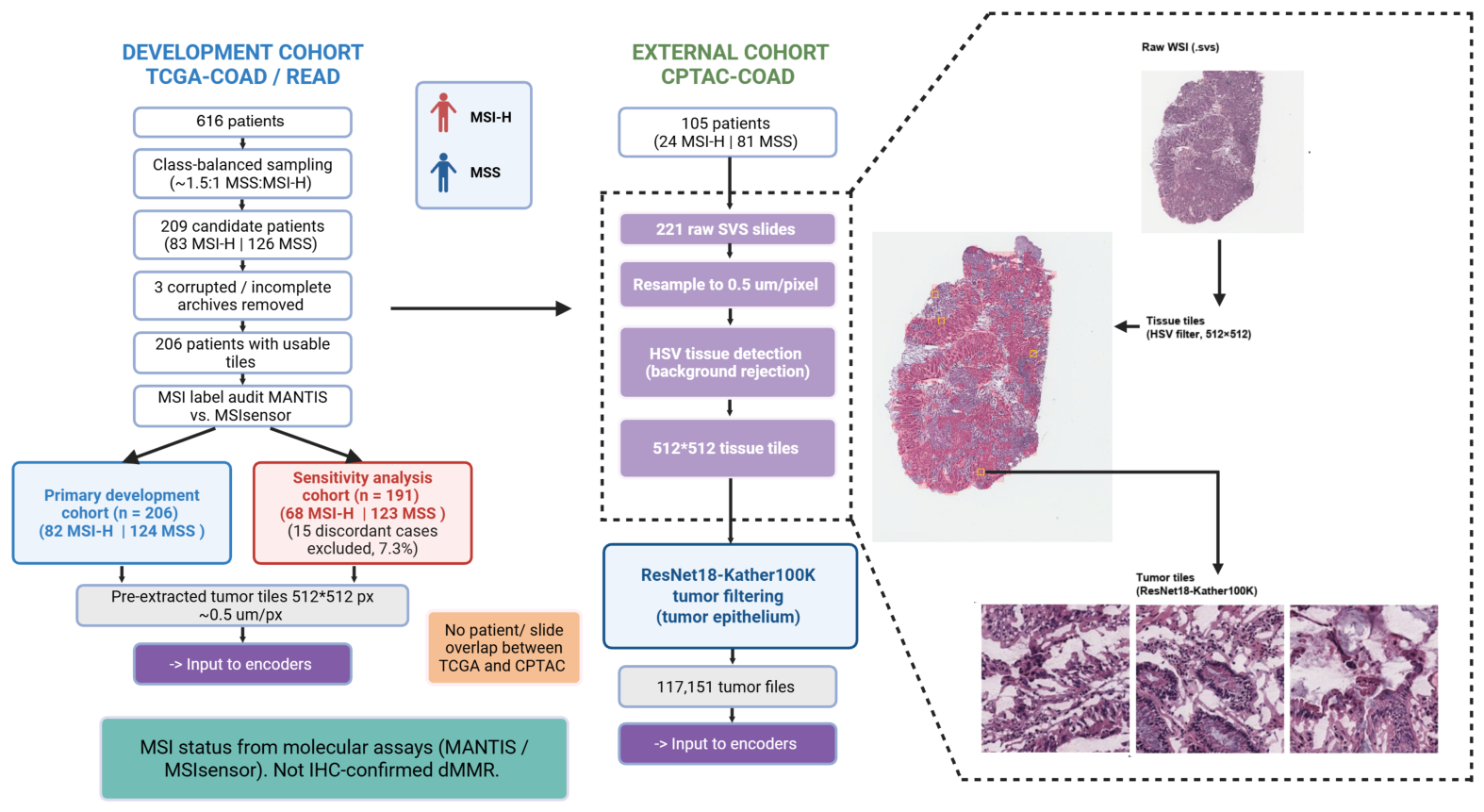
Candidate TCGA-COAD/READ patients were drawn from the TCGA-CRC-DX resource using class-balanced sampling from a 616-patient pool: all available MSI-H patients were retained, and MSS patients were randomly sampled at an approximate 1.5:1 MSS:MSI-H ratio (fixed seed 20260709), yielding 209 candidate patients (83 MSI-H, 126 MSS). Of these, 3 patients were subsequently dropped because of incomplete or corrupted tile archive downloads, leaving 206 patients with usable tile data. TCGA-CRC-DX tiles were provided as 512 × 512 pixel tumor tiles at approximately 0.5 μm/pixel, so no additional WSI tiling or tumor filtering was required for the development cohort.

The MSI labels for these 206 patients were derived from a MANTIS-score threshold, with MANTIS > 0.4 labeled MSI-H. The complete 206-patient cohort (82 MSI-H, 124 MSS) was retained as the primary development benchmark. A subsequent label provenance audit cross-referenced this labeling against independent MSIsensor scores and categorical MSI provenance and identified 15 of 206 patients (7.3%) as cross-source discordant. Fourteen patients had MANTIS scores above 0.4 but MSIsensor scores consistent with MSS (MSIsensor 0.00–2.26), while one patient had categorical MSI provenance despite a MANTIS score below 0.4 and a low MSIsensor score. To quantify the influence of this molecular-label discordance without relabeling the primary cohort after observing performance, we report the concordant-label 191-patient cohort (68 MSI-H, 123 MSS) as a secondary label provenance sensitivity analysis (Section 3.9). The improved sensitivity cohort performance should not be interpreted as evidence that the excluded cases were incorrectly labeled; rather, it illustrates the influence of molecular-label provenance on measured performance. This study therefore reports MSI-H prediction from molecular MSI-derived labels and does not claim IHC-confirmed mismatch-repair deficiency.

2.3. External Cohort

CPTAC-COAD was used as the independent external cohort after the data-readiness review. MSI status was obtained from the cBioPortal CPTAC-COAD study, where the usable MSI call was recorded under MUTATION_PHENOTYPE. The final external cohort included 105 patients, comprising 24 MSI-H and 81 MSS patients across 221 whole-slide images. Patients without a usable MSI label were excluded. The nominal MMR status was unknown for the external cohort; therefore, all external analyses used MSI-H versus MSS as the endpoint. An overlap audit confirmed no shared patient or slide identifiers between the TCGA development cohort and the CPTAC external cohort.

CPTAC-COAD images were downloaded as raw SVS whole-slide images. Unlike TCGA-CRC-DX, CPTAC-COAD required local tiling and tumor tile filtering. Whole-slide images were tiled at a target resolution of 0.5 μm/pixel to match the TCGA tile scale. Foreground tissue tiles were generated as 512 × 512 pixel images after HSV saturation-based background rejection. A separate tumor-filtering step then retained tiles predicted as tumor epithelium by the tiatoolbox ResNet18-Kather100K tissue classifier. This produced 117,151 tumor tiles for the 105 externally evaluable patients (Figure 1).

2.4. Frozen Encoder Feature Extraction

Nine encoders were evaluated as frozen feature extractors: CONCH, CONCH v1.5, UNI, Virchow2, Phikon, ResNet18, ResNet50, and ViT-B/16, pretrained on ImageNet-21k, and ConvNeXt-Tiny. For each encoder, tile embeddings were extracted without gradient updates. Patient-level features for linear probing were computed by mean-pooling tile embeddings to slide level and then mean-pooling slide embeddings to patient level, so each slide contributed equally to the patient-level representation, regardless of its tile count. This aggregation choice was intentionally simple, deterministic, and identical across encoders, so that the comparison assessed the downstream task utility of each frozen representation under the same aggregation and classifier protocol rather than isolating representation quality as a causal factor.

Because some pathology foundation models are pretrained on public histopathology resources that may overlap common downstream benchmarks, we performed a source-level pretraining provenance audit using public model cards, repositories, and associated papers (

Table 1. Source-level pretraining provenance audit for the evaluated encoders. The audit assesses dataset-level overlap risk from public sources; it does not establish patient- or slide-level independence when pretraining manifests are unavailable.

Encoder	Reported Public Pretraining Provenance	TCGA/CPTAC Overlap Interpretation
CONCH	1.17 million histopathology image–caption pairs; public model documentation states that large public histology slide collections including TCGA were not used [22,48].	Low dataset-level TCGA/CPTAC overlap risk based on public documentation; patient- and slide-level overlap cannot be determined from publicly available pretraining manifests.
CONCH v1.5	Based on CONCH and restored from UNI before similar vision–language fine-tuning [49].	No explicit TCGA/CPTAC use reported in the public model card; patient- and slide-level overlap cannot be determined from publicly available pretraining manifests.
UNI	Mass-100K from MGH, BWH, and GTEx; public model documentation states that TCGA, CPTAC, PAIP, CAMELYON, PANDA, and TCIA were not used for pretraining [21,50].	Low dataset-level TCGA/CPTAC overlap risk based on public documentation; patient- and slide-level overlap cannot be determined from publicly available pretraining manifests.
Virchow2	3.1 million whole-slide histopathology images from large-scale pathology pretraining [30,51].	No explicit TCGA/CPTAC use found in reviewed public sources; patient- and slide-level overlap cannot be determined from publicly available pretraining manifests.
Phikon	Public release describes Phikon as pretrained on 40 million pan-cancer histology tiles from TCGA [29,52].	High dataset-level TCGA overlap risk; patient- and slide-level overlap cannot be determined from publicly available pretraining manifests, so a sensitivity analysis excluding Phikon was performed.
Conventional backbones	Natural-image ImageNet or ImageNet-21k pretraining.	No pathology pretraining and no TCGA/CPTAC overlap expected.

). This audit was designed to identify dataset-level overlap risk. It cannot prove patient- or slide-level independence for encoders whose pretraining manifests are not public.

For attention–MIL experiments, per-tile embeddings were retained as patient-level bags. When a patient had multiple slides, all tiles from that patient’s slides were concatenated into one bag. This matched the patient-level unit used by the linear probe analysis and avoided slide-level leakage across cross-validation folds.

2.5. Linear Probe and Nonlinear Classifier Benchmark

Each encoder was evaluated on the TCGA development cohort using patient-level stratified 5-fold cross-validation with shuffling and a fixed random seed of 20260709. For every fold, the training and test patient sets were explicitly checked to be disjointed. Features were standardized within the training fold and transformed into the held-out fold. The primary linear probe was logistic regression with maximum 2000 iterations, balanced class weights, and the same random seed. Three nonlinear comparators were trained on the same patient embeddings: radial-basis-function support vector machine with probability output and balanced class weights, XGBoost with 200 estimators, maximum depth 3, learning rate 0.05, and log-loss evaluation, and 5-nearest-neighbor classification.

Pooled out-of-fold predictions were used to compute AUROC, AUPRC, sensitivity, specificity, accuracy, and F1 score. The default threshold for these internal classifier metrics was 0.5 and was not interpreted as a clinical rule-out threshold. To quantify linear separability, we defined the linear-separability gap for each encoder as:

$${\Delta }_{\mathrm{nonlinear}-\mathrm{linear}}={\mathrm{AUROC}}_{\mathrm{best} \mathrm{nonlinear}}-{\mathrm{AUROC}}_{\mathrm{logistic} \mathrm{regression}}.$$

(1)

A near-zero or negative value indicates that the frozen embedding is already linearly separable for the MSI-H task.

2.6. Representation Geometry, Similarity, and Calibration

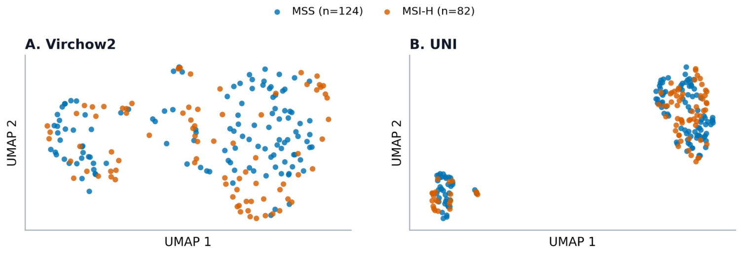
UMAP projections were generated from patient-level embeddings for qualitative visualization of class geometry, using 15 neighbors and a minimum distance of 0.1. These plots were used as qualitative support only and were not treated as primary statistical evidence.

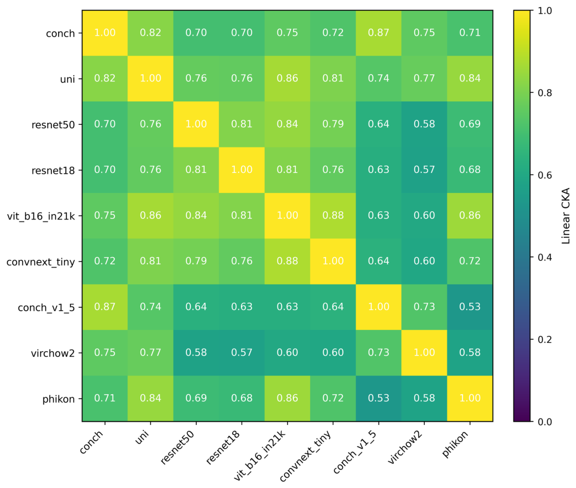
Pairwise linear centered-kernel alignment (CKA) was computed across all encoders after row-aligning patient embeddings by patient identifier. For column-centered embedding matrices $X_c$ and $Y_c$, linear CKA was defined as:

$$\mathrm{CKA}(X,Y)={\displaystyle \frac{{\parallel X_c^{\top }{Y}_c\parallel }_F^2}{{\parallel X_c^{\top }{X}_c\parallel }_F{\parallel Y_c^{\top }{Y}_c\parallel }_F}}.$$

(2)

Calibration was assessed on pooled out-of-fold predictions using the Brier score, mean predicted probability, calibration intercept, and calibration slope for every encoder–classifier pair. Calibration curves were generated with quantile binning. Calibration intercept and slope were estimated by fitting a logistic calibration model with the logit-transformed predicted probability as the only covariate.

2.7. Attention–MIL Comparator

To test whether a trained nonlinear tile aggregator improved over simple patient-level linear probing, we trained a gated-attention multiple-instance learning model for each encoder using CLAM_SB. The model used gated attention, the small CLAM configuration, a dropout of 0.25, k_sample = 8, two output classes, and encoder-specific embedding dimensionality. Training used the same patient-level stratified 5-fold split seed as the linear probe analysis. Each fold was trained for 20 epochs with Adam optimization, a learning rate of $2\times {10}^{-4}$, and weight decay of $1\times {10}^{-5}$. The loss combined bag-level cross-entropy and CLAM instance-level loss with weights of 0.7 and 0.3, respectively; for rare patients with fewer than eight tiles, instance-level supervision was skipped and bag-level loss alone was used. Fold checkpoints were saved separately and pooled out-of-fold predictions were used for evaluation.

2.8. External Validation and Local Threshold Adaptation

For external linear probe evaluation, each encoder’s final logistic regression pipeline was fit on the 206-patient primary development cohort and applied unchanged to CPTAC-COAD patient-level embeddings. A TCGA-locked threshold was selected from the development out-of-fold predictions at target sensitivity 0.93 and then applied to the external cohort without refitting. The 0.93 internal target was selected as an illustrative high-sensitivity operating point for exploratory prescreening analysis, rather than as a guideline-derived or clinically validated requirement. Discrimination metrics were reported independently from threshold metrics, because AUROC can transport even when the probability scale and decision threshold do not.

For the CONCH attention–MIL external experiment, the five fold checkpoints trained on the 206-patient cohort were loaded without weight updates and applied to each CPTAC patient bag. The five fold probabilities were averaged into one ensemble probability per patient. The locked TCGA threshold for the CONCH attention–MIL model was 0.000577, chosen from TCGA out-of-fold predictions at target sensitivity 0.93.

Local threshold adaptation was evaluated as a threshold-only simulation. In each of the 100 repeats, 15 MSI-H and 30 MSS CPTAC patients were drawn without replacement as a site-local threshold-adaptation subset, and the decision threshold was reselected on that subset at a target sensitivity of 0.90. The 0.90 target was also an illustrative high-sensitivity operating point and should not be interpreted as an endorsed clinical sensitivity target. The remaining 9 MSI-H and 51 MSS patients were held out for evaluation. Predicted probabilities and model weights were never updated, so this analysis is not a formal probability recalibration. Because the external cohort contained only 24 MSI-H patients, repeat-level threshold-adaptation subsets necessarily overlapped substantially; therefore, percentile intervals from the 100 repeats were interpreted as exploratory uncertainty summaries rather than independent validation intervals.

2.9. Statistical Analysis

Uncertainty in the primary group-level comparison was estimated with patient-level paired bootstrap resampling. For each of 2,000 bootstrap replicates, the same 206 TCGA patients were sampled with replacement, AUROC was recomputed for every encoder’s logistic regression out-of-fold predictions, the mean AUROC across the five pathology-specific encoders was computed, the mean AUROC across the four conventional encoders was computed, and the difference

$$\Delta ={\mathrm{AUROC}}_{\mathrm{pathology}}-{\mathrm{AUROC}}_{\mathrm{conventional}}$$

(3)

was recorded. Because the encoders were selected models rather than random experimental units sampled from broader pathology-specific and conventional model populations, this grouped comparison was interpreted descriptively and not as a formal class-level hypothesis test. Analyses were performed at the patient level.

2.10. Interpretability Artifacts

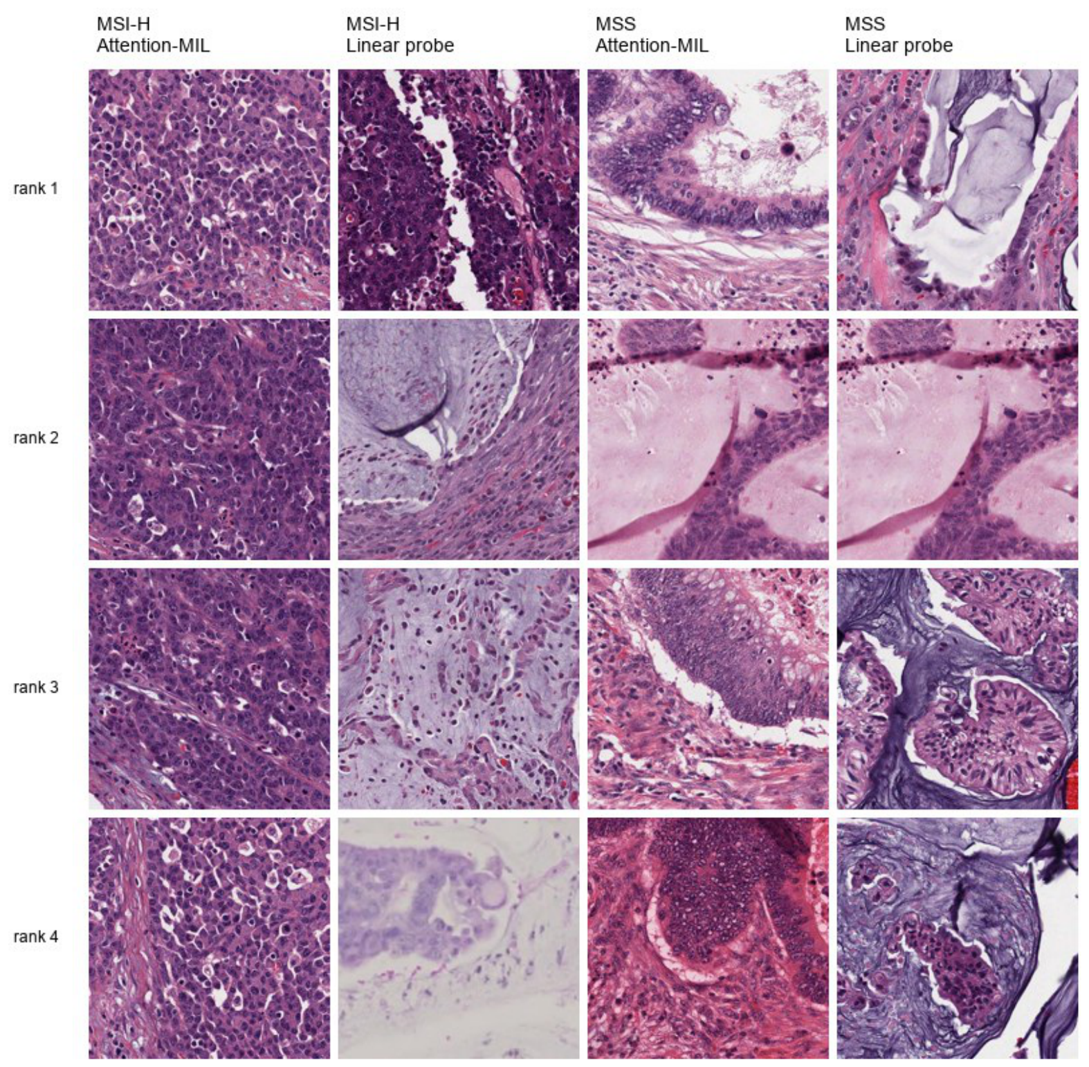
Top-tile exports were generated to support later morphological review. The tiles were ranked in two complementary ways: attention–MIL ranking by learned attention weight and linear probe ranking by the dot product between per-tile embeddings and the scaled logistic regression coefficient vector. Exported tile images and manifests preserve patient, slide, coordinate, label, encoder, and ranking provenance. These tile exports are interpretability artifacts for pathologist review and are not yet presented as validated biological findings.

3. Results

3.1. Cohort Processing Produced Matched Patient-Level Representations

The primary development benchmark included 206 TCGA patients (82 MSI-H, 124 MSS) with MANTIS-defined MSI labels. The secondary concordant-label sensitivity cohort included 191 patients (68 MSI-H, 123 MSS) after excluding 15 patients with cross-source MSI provenance discordance. All nine encoders produced patient-level embeddings for the same primary patient set, enabling direct paired comparison of out-of-fold predictions. The external CPTAC-COAD cohort included 105 patients, with 24 MSI-H and 81 MSS cases. CPTAC preprocessing retained 117,151 tumor tiles from 221 slides, and all nine encoders produced 105 patient-level external embeddings.

3.2. Pathology-Specific Foundation Models Provided Stronger Linear Probe Representations

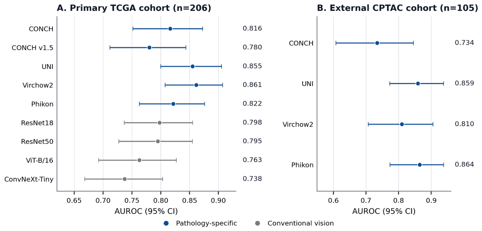
Under the fixed frozen feature logistic regression protocol in the primary n = 206 cohort, the highest internal AUROC was achieved by Virchow2 (0.861), followed by UNI (0.855), Phikon (0.822), CONCH (0.816), and ResNet18 (0.798) (

Table 2. Internal TCGA linear probe benchmark, primary cohort (n = 206). All encoders were evaluated with the same patient-level logistic regression probe on mean-pooled frozen embeddings. Sensitivity and specificity use the default 0.5 logistic regression threshold and are not clinical rule-out thresholds.

Encoder	Group	AUROC	AUPRC	Sensitivity	Specificity
Virchow2	Pathology-specific	0.861	0.819	0.744	0.839
UNI	Pathology-specific	0.855	0.788	0.720	0.806
Phikon	Pathology-specific	0.822	0.751	0.683	0.774
CONCH	Pathology-specific	0.816	0.771	0.683	0.790
ResNet18	Conventional	0.798	0.676	0.671	0.742
ResNet50	Conventional	0.795	0.714	0.695	0.766
CONCH v1.5	Pathology-specific	0.780	0.689	0.756	0.726
ViT-B/16	Conventional	0.763	0.641	0.622	0.726
ConvNeXt-Tiny	Conventional	0.738	0.634	0.634	0.694

). The five selected pathology-specific encoders had a mean AUROC of 0.827, compared with 0.773 for the four selected conventional vision backbones. Patient-level paired bootstrap estimated a mean AUROC difference of +0.054 in favor of the pathology-specific encoder set, with a 95% interval from +0.015 to +0.094 (

Table 3. Patient-level paired-bootstrap comparison of selected pathology-specific and conventional frozen representations, primary cohort (n = 206). This is a descriptive selected-encoder comparison, not a formal hypothesis test about model classes.

Comparison	Point	p2.5	p97.5
Pathology-specific mean AUROC	0.827	0.772	0.874
Conventional mean AUROC	0.773	0.712	0.830
$\Delta$ AUROC	+0.054	+0.015	+0.094

). Because Phikon had explicit TCGA-derived pretraining provenance in public sources (Table 1), we repeated the grouped comparison after excluding Phikon; the pathology-specific mean AUROC remained 0.828 versus 0.773 for conventional encoders, with a descriptive paired-bootstrap difference of +0.055 (95% interval, +0.014 to +0.098). Because the encoders were deliberately selected rather than sampled as exchangeable experimental units, these results are reported as descriptive uncertainty summaries for the selected encoders, not as formal inference about all pathology-specific or conventional model classes.

Figure 2 summarizes the primary internal linear probe benchmark and selected external CPTAC validation results using the revised cohort hierarchy. The figure is intended as a visual summary of the tabulated patient-level AUROC results; the full internal and external metric tables remain the primary numerical record.

3.3. Several High-Performing Embeddings Were Already Linearly Separable

Nonlinear classifiers did not consistently improve over logistic regression (

Table 4. Linear separability of frozen patient embeddings, primary cohort (n = 206). The gap is AUROC (best nonlinear classifier) minus AUROC (logistic regression).

Encoder	Best Nonlinear Model	LR AUROC	Best Nonlinear AUROC	Gap
ResNet18	SVM-RBF	0.798	0.777	−0.021
ResNet50	SVM-RBF	0.795	0.787	−0.007
Virchow2	SVM-RBF	0.861	0.856	−0.006
UNI	SVM-RBF	0.855	0.853	−0.003
ViT-B/16	SVM-RBF	0.763	0.768	+0.006
Phikon	XGBoost	0.822	0.832	+0.010
ConvNeXt-Tiny	SVM-RBF	0.738	0.762	+0.025
CONCH v1.5	SVM-RBF	0.780	0.809	+0.028
CONCH	XGBoost	0.816	0.856	+0.039

). ResNet18, ResNet50, Virchow2, and UNI had negative or near-zero linear-separability gaps, indicating that logistic regression matched or slightly exceeded the best nonlinear classifier tested here. CONCH showed the largest nonlinear gain: XGBoost improved AUROC from 0.816 to 0.856, a gap of +0.039. CONCH v1.5 also improved with SVM-RBF, from 0.780 to 0.809 (+0.028). These results indicate that the tested nonlinear configurations did not consistently improve performance for the strongest frozen representations, though nonlinear models remain meaningful comparators for some encoders.

3.4. Representation Geometry and Calibration Supported the Linear Probe Ranking

The UMAP projections provided qualitative visual support for the quantitative ranking of the frozen representations (Figure 3). CKA analysis on the primary n = 206 cohort showed that encoders did not collapse to a single shared representation geometry (Figure 4). The highest overall pairwise CKA was observed between ViT-B/16 and ConvNeXt-Tiny (0.878), both conventional transformer-like or modern ImageNet-derived backbones. Among pathology-specific encoders, CONCH and CONCH v1.5 were highly similar (CKA 0.869), and UNI and Phikon were also similar (CKA 0.845). Virchow2 had the lowest average similarity to the other encoders (mean off-diagonal CKA approximately 0.647), despite achieving the highest linear probe AUROC, suggesting that its representation captures MSI-relevant morphology through a distinct embedding geometry.

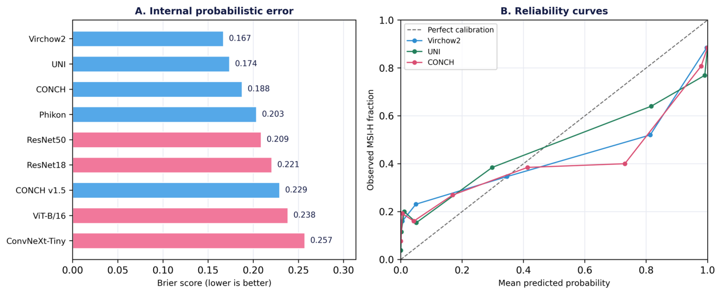
Calibration analysis on pooled out-of-fold predictions was consistent with the discrimination results but also highlighted that discrimination and probability calibration are not interchangeable (Figure 5). Among logistic regression probes, the lowest Brier score was observed for Virchow2 (0.167), followed by UNI (0.174) and CONCH (0.188). The corresponding calibration slopes were below 1.0 for all three models (Virchow2 0.235, UNI 0.264, CONCH 0.272), indicating that even internally strong models should not be interpreted as perfectly calibrated probability estimators. These diagnostics characterize probability scale behavior within the evaluated cohorts; they do not establish that the predicted probabilities represent prevalence-calibrated clinical risk, given the enriched development sampling and balanced class weighting.

3.5. Attention–MIL Did Not Establish a Need for Complex Downstream Models

Attention–MIL was evaluated as a trained nonlinear comparator using per-tile embedding bags (

Table 5. Attention–MIL pooled out-of-fold metrics on the TCGA development cohort, primary cohort (n = 206).

Encoder	AUROC	AUPRC	Sensitivity	Specificity
CONCH	0.855	0.804	0.707	0.879
Virchow2	0.846	0.798	0.756	0.823
UNI	0.843	0.796	0.695	0.847
CONCH v1.5	0.837	0.797	0.720	0.815
Phikon	0.823	0.761	0.707	0.790
ResNet50	0.741	0.608	0.598	0.702
ViT-B/16	0.738	0.663	0.573	0.774
ConvNeXt-Tiny	0.711	0.579	0.598	0.702
ResNet18	0.694	0.557	0.683	0.613

). CONCH attention–MIL had the highest pooled out-of-fold AUROC (0.855), followed by Virchow2 (0.846), UNI (0.843), and CONCH v1.5 (0.837). Attention–MIL improved performance for some encoders, including CONCH (0.816 linear probe vs. 0.855 attention–MIL) and CONCH v1.5 (0.780 vs. 0.837), but did not improve performance for Virchow2 or UNI. Overall, these results show that the specific nonlinear classifiers and CLAM configuration tested here did not establish a consistent practical advantage over linear probing.

3.6. External Validation Revealed Encoder-Specific Transportability

Scope note: The primary n = 206 pipeline trained and evaluated all nine linear probes and the CONCH attention–MIL model on the MANTIS-defined development cohort, then applied the frozen TCGA-trained models to CPTAC-COAD. Because TCGA used pre-extracted tumor tiles whereas CPTAC required local whole-slide tiling, foreground detection, and tumor tile filtering, the external analysis evaluates transportability of the complete analytical pipeline rather than the frozen encoder alone.

All nine linear probes, trained on the 206-patient primary development cohort, were applied to the independent CPTAC-COAD cohort using TCGA-trained frozen probes. External AUROC varied substantially by encoder (

Table 6. Frozen external validation of all nine TCGA-trained linear probes on CPTAC-COAD (probes trained on the primary n = 206 development cohort). Delta is external AUROC minus internal TCGA AUROC.

Encoder	Internal AUROC (n = 206)	External AUROC	Delta
Phikon	0.822	0.864	+0.042
UNI	0.855	0.859	+0.004
Virchow2	0.861	0.810	−0.051
CONCH	0.816	0.734	−0.082
ResNet50	0.795	0.705	−0.090
ViT-B/16	0.763	0.689	−0.074
CONCH v1.5	0.780	0.625	−0.155
ConvNeXt-Tiny	0.738	0.582	−0.156
ResNet18	0.798	0.574	−0.225

). Phikon achieved the highest external linear probe AUROC (0.864), followed by UNI (0.859) and Virchow2 (0.810). These results distinguish internal linear probe discrimination from external transportability of the full preprocessing-and-prediction pipeline.

External calibration diagnostics further showed that discrimination and probability calibration were not interchangeable (

Table 7. External CPTAC-COAD calibration diagnostics for principal n = 206-trained models. Calibration intercept and slope were estimated by logistic calibration of the observed label on the logit-predicted probability.

Model	Mean P	AUROC	Brier	Cal. Int.	Cal. Slope
CONCH attention–MIL	0.615	0.880	0.289	−2.485	0.730
Phikon linear probe	0.796	0.864	0.512	−3.552	0.433
UNI linear probe	0.725	0.859	0.445	−3.196	0.514
Virchow2 linear probe	0.397	0.810	0.213	−1.341	0.224

). The CPTAC-COAD-observed MSI-H prevalence was 0.229, while the mean predicted probabilities varied from 0.397 for Virchow2 to 0.796 for Phikon among the principal external linear probes. Calibration slopes below 1.0 indicated compressed or shifted probability behavior relative to ideal calibration, even for models with strong AUROC.

3.7. Frozen Discrimination Transported Better than Frozen Thresholds

The n = 206-trained CONCH attention–MIL model achieved external AUROC 0.880 on CPTAC-COAD, indicating preserved discrimination under the full preprocessing-and-prediction pipeline. However, the TCGA-locked threshold (0.000577, target sensitivity 0.93) did not transport: specificity was 0.000 at the frozen threshold, consistent with calibration or probability scale shift rather than a complete loss of discrimination (

Table 8. Threshold transportability for the n = 206-trained CONCH attention–MIL model. The same TCGA-locked threshold was applied to pooled TCGA out-of-fold predictions and to frozen CPTAC ensemble predictions without model updating. Sensitivity and specificity are computed at the locked threshold; medians are predicted MSI-H probabilities within each label group.

Cohort	Prediction Set	n	AUROC	Thr.	Sens.	Spec.	Median MSS	Median MSI-H
Primary TCGA	Pooled OOF	206	0.855	0.000577	0.939	0.411	0.002	0.975
External CPTAC	Frozen ensemble	105	0.880	0.000577	1.000	0.000	0.571	0.986

).

Threshold-only local adaptation recovered specificity for several models without updating predicted probabilities or model weights (

Table 9. Local threshold adaptation on CPTAC-COAD. Each repeat used 15 MSI-H and 30 MSS patients for threshold selection and evaluated the remaining 9 MSI-H and 51 MSS patients. Values are medians across 100 repeats. All rows use models trained on the primary n = 206 development cohort.

Model	Frozen AUROC	Frozen Spec.	Adapt. Sens.	Adapt. Spec.
CONCH attention–MIL (n = 206)	0.880	0.000	0.889	0.686
UNI linear probe (n = 206)	0.859	0.037	0.889	0.765
Virchow2 linear probe (n = 206)	0.810	0.185	0.889	0.480

). For the n = 206-trained CONCH attention–MIL model, the median threshold-adapted sensitivity was 0.889 and the median specificity was 0.686. The n = 206-trained UNI and Virchow2 linear probes achieved median threshold-adapted specificities of 0.765 and 0.480, respectively. These results support a deployment framing in which discrimination, probability calibration, and site-local threshold selection are reported separately, not a fully frozen end-to-end threshold claim.

The CPTAC probability summaries from individual CONCH attention–MIL fold checkpoints were non-degenerate and broadly consistent with the ensemble pattern (

Table 10. External CPTAC-COAD fold-checkpoint diagnostic for the n = 206-trained CONCH attention–MIL model. All sensitivity and specificity values use the same TCGA-locked threshold of 0.000577; medians are predicted MSI-H probabilities within each label group.

Checkpoint	AUROC	Sens.	Spec.	Median MSS	Median MSI-H
Fold 1	0.771	1.000	0.000	0.781	0.998
Fold 2	0.878	1.000	0.025	0.132	0.970
Fold 3	0.874	1.000	0.025	0.271	0.998
Fold 4	0.753	1.000	0.000	0.845	0.992
Fold 5	0.871	1.000	0.012	0.892	1.000
Ensemble	0.880	1.000	0.000	0.571	0.986

). This diagnostic supports the interpretation that the frozen-threshold failure was not driven by a single anomalous fold checkpoint, while still leaving open contributions from external preprocessing, cohort composition, and probability scale shift.

3.8. Rule-Out Simulation Illustrates the Cost of Small External MSI-H Counts

The detailed per-1000 rule-out projection has been moved to Supplementary Table S1. Briefly, using the observed CPTAC-COAD MSI-H prevalence of 24/105 (22.9%) and the n = 206-trained CONCH attention–MIL threshold-adaptation simulation, the median projection was 554.8 patients per 1000 ruled out, including 529.4 true MSS patients and 25.4 missed MSI-H patients. The uncertainty interval was wide: the 97.5th percentile reached 101.6 missed MSI-H patients per 1000. This reflects both the small number of external MSI-H cases and the high overlap among repeated threshold-adaptation subsets. Therefore, this analysis should be interpreted as an exploratory workflow simulation rather than evidence of clinical safety.

3.9. Concordant-Label Sensitivity Analysis

As a secondary label provenance sensitivity analysis, we re-examined the 191-patient concordant-label cohort after excluding the 15 MANTIS/MSIsensor-discordant patients from the primary n = 206 cohort. The AUROC of the strongest linear probes increased in the concordant-label cohort: Virchow2 increased from 0.861 to 0.926, UNI from 0.855 to 0.928, Phikon from 0.822 to 0.890, and CONCH from 0.816 to 0.869 (

Table 11. Sensitivity analysis: effect of excluding 15 TCGA patients with discordant MSI label provenance from the primary n = 206 cohort.

Encoder	Primary AUROC (n = 206)	Concordant-Label AUROC (n = 191)	Delta
Virchow2	0.861	0.926	+0.065
UNI	0.855	0.928	+0.073
Phikon	0.822	0.890	+0.068
CONCH	0.816	0.869	+0.053

). This sensitivity analysis shows that molecular-label provenance materially affects apparent discrimination, but it should not be interpreted as proof that the discordant cases were incorrectly labeled or as justification for redefining the higher-performing subset as the primary cohort.

3.10. Top-Tile Exports Provide Reviewable Morphological Evidence

For each encoder, top-ranked MSI-H and MSS tiles were exported using both attention–MIL weights and linear probe coefficient scores. These images are available as reviewable artifacts with patient, slide, coordinate, encoder, and ranking provenance. At the present draft stage, these exports support qualitative pathologist review but are not yet interpreted as validated morphological mechanisms. Representative UNI examples are shown in Figure 6 to illustrate the interpretability workflow. Because these tiles were not independently annotated by pathologists, they are presented solely as exploratory artifacts and are not interpreted as evidence of specific MSI-associated histopathological mechanisms.

4. Discussion

This study provides evidence for the ability to predict MSI-H from colorectal cancer histopathology using nine frozen image encoders. First, the discriminative performance of frozen representations varied substantially across the nine encoders when compared within the same standardized linear probe framework. Several encoders pretrained on large-scale histopathology images, particularly Virchow2 and UNI, generated representations that better discriminated MSI-H from MSS than conventional vision backbones, with AUROCs of 0.861 and 0.855, respectively, whereas other pathology-specific models and conventional vision architectures showed lower discriminative performance. This suggests that pretraining on large-scale histopathology data may enable encoders to learn morphological features related to the glandular architecture, tumor differentiation, lymphocytic infiltration, and tumor microenvironment that are associated with MSI-H and can still be exploited by a simple linear classifier [53,54,55,56]. However, the advantage of pathology-specific pretraining was not uniform across all models. The CONCH v1.5 encoder achieved an AUROC of 0.780, lower than several conventional backbones such as ResNet18 and ResNet50, whose underlying architectural families were originally developed for general computer vision tasks [57,58]. Therefore, the results do not support an absolute conclusion that every pathology foundation model outperforms conventional vision models. Instead, they indicate a descriptive, group-level advantage among the selected encoders, accompanied by substantial variability across individual encoders. Representation quality may depend not only on whether a model was pretrained on pathology data, but also on the scale and composition of the pretraining dataset and the self-supervised objective [21,22,23,24,25,26,27,28], as well as model architecture, image resolution, and sampling strategy during pretraining [29,30]. Previous studies have demonstrated the utility of pathology-pretrained models designed to learn morphological representations across a variety of downstream tasks [21,22,24,25,26,27,28,32,59]. More recent standardized benchmarks have also shown that the relative ranking of pathology foundation models can vary across datasets, prediction tasks, sample sizes, and downstream adaptation strategies [31,32,33,34,35].

Second, a label provenance audit of the development cohort showed that discrimination performance was sensitive to the molecular MSI label definition. The as-collected TCGA-CRC-DX cohort of 206 patients used a single MANTIS-score threshold to assign MSI-H status; cross-referencing this labeling against independent MSIsensor scores and categorical MSI provenance identified 15 of 206 patients (7.3%) with cross-source discordance. We retained the complete MANTIS-defined 206-patient cohort as the primary development benchmark and report the 191-patient concordant-label cohort only as a secondary sensitivity analysis (Table 11). AUROC for the strongest linear probes increased in the concordant-label cohort: UNI increased from 0.855 to 0.928, Virchow2 from 0.861 to 0.926, Phikon from 0.822 to 0.890, and CONCH from 0.816 to 0.869. This pattern indicates that molecular-label provenance materially affects apparent discrimination. However, it should not be interpreted as proof that the discordant cases were incorrectly labeled or as evidence that the higher-performing concordant subset should replace the originally specified full MANTIS-defined cohort as the primary benchmark.

Third, the results showed that in the primary development cohort of 206 patients, Virchow2 and UNI achieved the strongest discrimination with linear probes, with AUROCs of 0.861 and 0.855, respectively, while nonlinear classifiers did not further improve performance for these two encoders. Specifically, the best nonlinear AUROCs for Virchow2 and UNI were 0.856 and 0.853, corresponding to linear-separability gaps of $-0.006$ and $-0.003$. In contrast, some encoders, such as CONCH and CONCH v1.5, improved when nonlinear classifiers were used, with AUROC increasing from 0.816 to 0.856 for CONCH and from 0.780 to 0.809 for CONCH v1.5. This suggests that the benefit of nonlinear decision boundaries depends on the characteristics of the representation generated by each encoder rather than reflecting a general advantage of nonlinear models. A similar pattern was observed when comparing linear probes with attention–MIL. Attention–MIL improved performance for some encoders, particularly CONCH and CONCH v1.5, with AUROC increasing from 0.816 to 0.855 and from 0.780 to 0.837, respectively, but did not provide a consistent benefit across the remaining models. For Virchow2 and UNI, the two encoders with the highest linear probe performance, attention–MIL produced lower AUROCs than the linear probes (0.846 vs. 0.861 for Virchow2 and 0.843 vs. 0.855 for UNI). For several other backbones, performance also decreased after the use of attention–MIL, including ResNet18 (0.798 to 0.694), ViT-B/16 (0.763 to 0.738), and ConvNeXt-Tiny (0.738 to 0.711); ConvNeXt represents a modernized convolutional architecture originally developed for general computer vision [60]. Overall, increasing downstream model complexity through the tested nonlinear classifiers or the tested attention–MIL configuration did not provide consistent improvement over a simple linear probe. Therefore, the results do not support the assumption that using a more complex downstream architecture automatically leads to better MSI-H discrimination.

One possible explanation is that strong frozen representations had already encoded most of the MSI-H-related morphological signal in a manner that could be effectively exploited by a simple linear decision boundary. In this situation, more complex models increase the number of parameters to be estimated, dependence on hyperparameters, variability arising from optimization, and the risk of overfitting, particularly when the patient-level sample size remains limited [32,33,61]. A linear probe may therefore be considered an important and practically useful baseline because of its simple architecture, low computational cost, and favorable reproducibility. However, these results do not demonstrate that linear models are generally superior to attention–MIL, because some encoders, such as CONCH and CONCH v1.5, still benefited from greater downstream complexity. Attention–MIL remains architecturally valuable because it can aggregate variable numbers of tiles across patients and learn different weights for individual tiles rather than treating all tiles as equally important [36,37,38]. Recent benchmarking studies of pathology foundation models have also shown that downstream performance depends not only on the complexity of the aggregator but also strongly on the quality of the frozen representation, the type of task, and the cohort being evaluated [31,32,33,34]. Some benchmarks have shown that relatively simple aggregation methods can remain competitive with newer and more complex architectures [32,33,34], emphasizing that architectural complexity should not be regarded as a direct proxy for predictive quality.

Fourth, the three components of discrimination, predicted-probability calibration, and the transportability of thresholds derived from the development cohort were not necessarily preserved simultaneously when the model was applied to external data. In the independent CPTAC-COAD dataset, CONCH attention–MIL trained on the primary development cohort still maintained relatively good discrimination, with an AUROC of 0.880. However, the threshold derived from TCGA did not produce a meaningful binary classification when directly applied to CPTAC-COAD, with a specificity equal to 0. This indicates that the ability to rank MSI-H cases above MSS cases was preserved to some extent, whereas the development-derived threshold did not transport to the new cohort. This finding is consistent with established prediction model methodology, showing that discrimination and calibration characterize different aspects of predictive performance [44,45,46,47]. AUROC primarily reflects the relative ranking ability between individuals with and without an outcome, whereas calibration reflects the agreement between predicted probabilities and observed outcome frequencies. Therefore, a model may maintain relatively good discrimination while failing to preserve the same probability scale or decision threshold when transported to another population.

Differences between cohorts in tissue processing, H&E staining, scanners, image resolution, case mix, and tissue region selection are recognized sources of distributional variation and domain shift in computational pathology [40,41,42,43]. In this study, the probability distribution of MSS cases in TCGA was concentrated near 0, whereas in CPTAC, it was distributed much more broadly across the probability scale, suggesting a change in probability scale between the two cohorts. We also found no clear evidence of label inversion, extraction of the wrong probability column, application of softmax along the wrong dimension, or checkpoint–loading incompatibility; probabilities were obtained from the correct MSI-H class, and the external AUROCs across folds were directionally consistent rather than suggesting that one fold had been abnormally inverted. These checks reduce the likelihood that the specificity of 0 was simply the consequence of a basic coding error. However, the current results also do not allow the entire threshold failure to be attributed to domain shift, because prediction generation differed between development and external evaluation. The development threshold was derived from out-of-fold predictions, whereas the external prediction was generated by averaging probabilities from five fold-specific models. These two mechanisms do not necessarily produce the same probability distribution, and prediction model methodology emphasizes that calibration and operating characteristics must be evaluated for the actual model implementation used in the target population [45,46,62,63]. Therefore, part of the threshold failure may result from incompatibility between the prediction-generating procedures in addition to genuine differences between the two cohorts. After the threshold was reselected within the CPTAC threshold-adaptation subsets, the specificity of CONCH attention–MIL improved from 0 to a median of 0.686, while median sensitivity was maintained at 0.889. This suggests that at least part of the failure of the frozen threshold was related to the position of the operating point or a shift in probability scale rather than a complete loss of discrimination. However, this improvement remained insufficient to establish a clinically deployable threshold. Furthermore, this analysis represented threshold-only adaptation rather than formal probability recalibration; reselection of the threshold does not automatically correct the relationship between predicted probability and observed event frequency [47,62,63].

Interpretation of the threshold-adaptation results was also limited by the small external sample size. CPTAC-COAD contained only 24 MSI-H cases, of which each repeat used 15 MSI-H cases for threshold selection and retained only nine MSI-H cases for evaluation. Therefore, a single misclassified case could change sensitivity by more than 11 percentage points. Contemporary methodological work has shown that the required sample size for external validation depends on the precision required for discrimination, calibration, and other performance measures rather than on a single universal event-count rule [64,65,66,67]. In addition, the same small number of patients was reused across 100 splits; each MSI-H patient appeared in the threshold-adaptation subset an average of approximately 62.5 times, and the overlap between any two splits was approximately 62.4%. Therefore, the percentiles obtained across the 100 repeats primarily reflect the sensitivity of the results to how the data were split rather than reproducibility across independent populations. These repeated splits do not increase the effective external sample size and cannot replace a larger external-validation cohort. More generally, performance in external populations can be affected by differences in case mix as well as by model misspecification [45,46,68]. Overall, the results indicate that discrimination may be better preserved than the transportability of the probability scale and decision threshold when a model is applied to an independent cohort. At the same time, stronger apparent discrimination in the concordant-label sensitivity cohort did not eliminate the problem of external threshold transportability. Therefore, external validation of pathology AI models should not rely solely on AUROC but should separately assess discrimination, calibration, and threshold-specific operating characteristics [45,46,53]. Establishing a deployable threshold should be performed in a sufficiently large calibration cohort and subsequently confirmed in a completely independent test cohort [64,65,66,67].

From a translational perspective, these findings support further investigation of histopathology-derived MSI-H scores as prescreening or prioritization tools, but they do not support replacement of reference molecular testing [3,13,14]. A proposed prescreening strategy should clearly define its intended use, acceptable false-negative rate, target population, and expected MSI-H prevalence. Measures such as the number of confirmatory tests avoided, the number of MSI-H tumors missed, and net clinical benefit provide more informative guidance for deployment decisions than discrimination alone [63,69,70]. We therefore moved the detailed per-1000 rule-out projection to Supplementary Table S1 and retained only a brief main-text summary. Using the observed MSI-H prevalence of 22.9% in CPTAC-COAD, the n = 206-trained CONCH attention–MIL-based strategy could avoid approximately 555 confirmatory tests per 1000 patients in the median scenario, but would simultaneously miss approximately 25 MSI-H cases. More importantly, uncertainty remained substantial, with the number of missed MSI-H cases at the 97.5th percentile reaching approximately 102 per 1000 patients. Therefore, the potential benefit of reducing the number of tests must be weighed against the risk of false-negative results, particularly for a strategy intended for rule-out purposes. These findings should be regarded as an exploratory simulation of workflow efficiency rather than evidence of clinical safety. Confirmation of model utility will require a prespecified threshold evaluated in a larger, completely independent external cohort with a sufficient number of MSI-H cases to provide stable estimates of sensitivity and the false-negative rate [65,67].

In the future, the study should be validated in larger and multicenter external cohorts with a sufficient number of MSI-H cases to allow precise estimation of discrimination, calibration, and decision threshold stability [64,65,66,67]. A more rigorous design should separate the cohort used for probability or threshold calibration from a completely independent test cohort used for final evaluation [45,62,63]. In addition, the effects of different tissue-region-selection strategies should be assessed, image-processing procedures should be standardized across cohorts, and blinded evaluation of highly weighted tiles should be performed by pathologists. The importance of controlling technical and institution-specific variation in digital pathology has been repeatedly demonstrated [40,41,42,43]. Future studies may also explore multimodal strategies that integrate pathology-derived representations with complementary clinical, imaging, or molecular information, as such frameworks have shown potential for improving clinically oriented prognostic modeling [71]. These steps will help determine whether the MSI-H signal learned from frozen pathology representations is sufficiently stable and clinically valuable to be developed into a prescreening tool for clinical support.

5. Conclusions

Among the selected encoders evaluated under this common framework, pathology-specific foundation models showed stronger average frozen-representation performance than conventional vision backbones, while more complex downstream classifiers did not consistently improve upon simple linear probes. Importantly, external discrimination was more robust than probability calibration and threshold transportability, indicating that favorable AUROC alone is insufficient to establish deployment readiness. These findings support frozen pathology representations as promising components of MSI-H prescreening pipelines but do not yet justify clinical rule-out use. Further multicenter validation with dedicated calibration and independent testing is required before clinical implementation.

References

1. Bray, F.; Laversanne, M.; Sung, H.; Ferlay, J.; Siegel, R.L.; Soerjomataram, I.; Jemal, A. Global cancer statistics 2022: GLOBOCAN estimates of incidence and mortality worldwide for 36 cancers in 185 countries. CA Cancer J. Clin. 2024, 74, 229–263. [Google Scholar] [CrossRef] [Scilit] [PubMed]
2. Boland, C.R.; Goel, A. Microsatellite instability in colorectal cancer. Gastroenterology 2010, 138, 2073–2087.e3. [Google Scholar] [CrossRef] [Scilit] [PubMed]
3. Sepulveda, A.R.; Hamilton, S.R.; Allegra, C.J.; Grody, W.; Cushman-Vokoun, A.M.; Funkhouser, W.K.; Kopetz, S.E.; Lieu, C.; Lindor, N.M.; Minsky, B.D.; et al. Molecular Biomarkers for the Evaluation of Colorectal Cancer: Guideline From the American Society for Clinical Pathology, College of American Pathologists, Association for Molecular Pathology, and the American Society of Clinical Oncology. J. Clin. Oncol. 2017, 35, 1453–1486. [Google Scholar] [CrossRef] [Scilit] [PubMed]
4. André, T.; Shiu, K.K.; Kim, T.W.; Jensen, B.V.; Jensen, L.H.; Punt, C.; Smith, D.; Garcia-Carbonero, R.; Benavides, M.; Gibbs, P.; et al. Pembrolizumab in Microsatellite-Instability-High Advanced Colorectal Cancer. N. Engl. J. Med. 2020, 383, 2207–2218. [Google Scholar] [CrossRef] [Scilit] [PubMed]
5. Le, D.T.; Uram, J.N.; Wang, H.; Bartlett, B.R.; Kemberling, H.; Eyring, A.D.; Skora, A.D.; Luber, B.S.; Azad, N.S.; Laheru, D.; et al. PD-1 Blockade in Tumors with Mismatch-Repair Deficiency. N. Engl. J. Med. 2015, 372, 2509–2520. [Google Scholar] [CrossRef] [Scilit] [PubMed]
6. Boland, C.R.; Thibodeau, S.N.; Hamilton, S.R.; Sidransky, D.; Eshleman, J.R.; Burt, R.W.; Meltzer, S.J.; Rodriguez-Bigas, M.A.; Fodde, R.; Ranzani, G.N.; et al. A National Cancer Institute Workshop on Microsatellite Instability for cancer detection and familial predisposition: Development of international criteria for the determination of microsatellite instability in colorectal cancer. Cancer Res. 1998, 58, 5248–5257. [Google Scholar] [PubMed]
7. Hampel, H.; Frankel, W.L.; Martin, E.; Arnold, M.; Khanduja, K.; Kuebler, P.; Clendenning, M.; Sotamaa, K.; Prior, T.; Westman, J.A.; et al. Feasibility of screening for Lynch syndrome among patients with colorectal cancer. J. Clin. Oncol. 2008, 26, 5783–5788. [Google Scholar] [CrossRef] [Scilit] [PubMed]
8. Hampel, H.; Frankel, W.L.; Martin, E.; Arnold, M.; Khanduja, K.; Kuebler, P.; Nakagawa, H.; Sotamaa, K.; Prior, T.W.; Westman, J.; et al. Screening for the Lynch syndrome (hereditary nonpolyposis colorectal cancer). N. Engl. J. Med. 2005, 352, 1851–1860. [Google Scholar] [CrossRef] [Scilit] [PubMed]
9. Trinh, H.D.; Pham, Q.T.; Phong, N.H.; Huong Ly, T.T.; Ho, Q.C.; Vu, H.A.; Kha, V.; Ngo, Q.D. Deficient Mismatch Repair Subtypes in Vietnamese Colorectal Cancer: Clinicopathologic Associations, Predictive Modeling, and IHC-PCR Concordance. Cancer Manag. Res. 2026, 18, 587649. [Google Scholar] [CrossRef] [Scilit] [PubMed]
10. Hechtman, J.F.; Middha, S.; Stadler, Z.K.; Zehir, A.; Berger, M.F.; Vakiani, E.; Weiser, M.R.; Ladanyi, M.; Saltz, L.B.; Klimstra, D.S.; et al. Universal screening for microsatellite instability in colorectal cancer in the clinical genomics era: New recommendations, methods, and considerations. Fam. Cancer 2017, 16, 525–529. [Google Scholar] [CrossRef] [Scilit] [PubMed]
11. Shaikh, T.; Handorf, E.A.; Meyer, J.E.; Hall, M.J.; Esnaola, N.F. Mismatch Repair Deficiency Testing in Patients With Colorectal Cancer and Nonadherence to Testing Guidelines in Young Adults. JAMA Oncol. 2018, 4, e173580. [Google Scholar] [CrossRef] [Scilit] [PubMed]
12. Steinberg, J.; Chan, P.; Hogden, E.; Tiernan, G.; Morrow, A.; Kang, Y.J.; He, E.; Venchiarutti, R.; Titterton, L.; Sankey, L.; et al. Lynch syndrome testing of colorectal cancer patients in a high-income country with universal healthcare: A retrospective study of current practice and gaps in seven australian hospitals. Hered. Cancer Clin. Pract. 2022, 20, 18. [Google Scholar] [CrossRef] [Scilit] [PubMed]
13. Vikas, P.; Messersmith, H.; Compton, C.; Sholl, L.; Broaddus, R.R.; Davis, A.; Estevez-Diz, M.; Garje, R.; Konstantinopoulos, P.A.; Leiser, A.; et al. Mismatch Repair and Microsatellite Instability Testing for Immune Checkpoint Inhibitor Therapy: ASCO Endorsement of College of American Pathologists Guideline. J. Clin. Oncol. 2023, 41, 1943–1948. [Google Scholar] [CrossRef] [Scilit] [PubMed]
14. Echle, A.; Ghaffari Laleh, N.; Quirke, P.; Grabsch, H.I.; Muti, H.S.; Saldanha, O.L.; Brockmoeller, S.; Brandt, P.v.D.; Hutchins, G.; Richman, S.; et al. Artificial intelligence for detection of microsatellite instability in colorectal cancer-a multicentric analysis of a pre-screening tool for clinical application. ESMO Open 2022, 7, 100400. [Google Scholar] [CrossRef] [Scilit] [PubMed]
15. Echle, A.; Grabsch, H.I.; Quirke, P.; van den Brandt, P.A.; West, N.P.; Hutchins, G.G.A.; Heij, L.R.; Tan, X.; Richman, S.D.; Krause, J.; et al. Clinical-Grade Detection of Microsatellite Instability in Colorectal Tumors by Deep Learning. Gastroenterology 2020, 159, 1406–1416.e11. [Google Scholar] [CrossRef] [Scilit] [PubMed]
16. Kather, J.N.; Pearson, A.T.; Halama, N.; Jäger, D.; Krause, J.; Loosen, S.H.; Marx, A.; Boor, P.; Tacke, F.; Neumann, U.P.; et al. Deep learning can predict microsatellite instability directly from histology in gastrointestinal cancer. Nat. Med. 2019, 25, 1054–1056. [Google Scholar] [CrossRef] [Scilit] [PubMed]
17. Lee, S.H.; Song, I.H.; Jang, H.J. Feasibility of deep learning-based fully automated classification of microsatellite instability in tissue slides of colorectal cancer. Int. J. Cancer 2021, 149, 728–740. [Google Scholar] [CrossRef] [Scilit] [PubMed]
18. Yamashita, R.; Long, J.; Longacre, T.; Peng, L.; Berry, G.; Martin, B.; Higgins, J.; Rubin, D.L.; Shen, J. Deep learning model for the prediction of microsatellite instability in colorectal cancer: A diagnostic study. Lancet Oncol. 2021, 22, 132–141. [Google Scholar] [CrossRef] [Scilit] [PubMed]
19. Guo, B.; Li, X.; Yang, M.; Jonnagaddala, J.; Zhang, H.; Xu, X.S. Predicting microsatellite instability and key biomarkers in colorectal cancer from H&E-stained images: Achieving state-of-the-art predictive performance with fewer data using Swin Transformer. J. Pathol. Clin. Res. 2023, 9, 223–235. [Google Scholar] [CrossRef] [Scilit] [PubMed]
20. Lou, J.; Xu, J.; Zhang, Y.; Sun, Y.; Fang, A.; Liu, J.; Ji, B. PPsNet: An improved deep learning model for microsatellite instability high prediction in colorectal cancer from whole slide images. Comput. Methods Programs Biomed. 2022, 225, 107095. [Google Scholar] [CrossRef] [Scilit] [PubMed]
21. Chen, R.J.; Ding, T.; Lu, M.Y.; Williamson, D.F.K.; Jaume, G.; Song, A.H.; Chen, B.; Zhang, A.; Shao, D.; Shaban, M.; et al. Towards a general-purpose foundation model for computational pathology. Nat. Med. 2024, 30, 850–862. [Google Scholar] [CrossRef] [Scilit] [PubMed]
22. Lu, M.Y.; Chen, B.; Williamson, D.F.K.; Chen, R.J.; Liang, I.; Ding, T.; Jaume, G.; Odintsov, I.; Le, L.P.; Gerber, G.; et al. A visual-language foundation model for computational pathology. Nat. Med. 2024, 30, 863–874. [Google Scholar] [CrossRef] [Scilit] [PubMed]
23. Vorontsov, E.; Bozkurt, A.; Casson, A.; Shaikovski, G.; Zelechowski, M.; Severson, K.; Zimmermann, E.; Hall, J.; Tenenholtz, N.; Fusi, N.; et al. A foundation model for clinical-grade computational pathology and rare cancers detection. Nat. Med. 2024, 30, 2924–2935. [Google Scholar] [CrossRef] [Scilit] [PubMed]
24. Xu, H.; Usuyama, N.; Bagga, J.; Zhang, S.; Rao, R.; Naumann, T.; Wong, C.; Gero, Z.; González, J.; Gu, Y.; et al. A whole-slide foundation model for digital pathology from real-world data. Nature 2024, 630, 181–188. [Google Scholar] [CrossRef] [Scilit] [PubMed]
25. Wang, X.; Zhao, J.; Marostica, E.; Yuan, W.; Jin, J.; Zhang, J.; Li, R.; Tang, H.; Wang, K.; Li, Y.; et al. A pathology foundation model for cancer diagnosis and prognosis prediction. Nature 2024, 634, 970–978. [Google Scholar] [CrossRef] [Scilit] [PubMed]
26. Ma, J.; Guo, Z.; Zhou, F.; Wang, Y.; Xu, Y.; Li, J.; Yan, F.; Cai, Y.; Zhu, Z.; Jin, C.; et al. A generalizable pathology foundation model using a unified knowledge distillation pretraining framework. Nat. Biomed. Eng. 2026, 10, 545–564. [Google Scholar] [CrossRef] [Scilit] [PubMed]
27. Ding, T.; Wagner, S.J.; Song, A.H.; Chen, R.J.; Lu, M.Y.; Zhang, A.; Vaidya, A.J.; Jaume, G.; Shaban, M.; Kim, A.; et al. A multimodal whole-slide foundation model for pathology. Nat. Med. 2025, 31, 3749–3761. [Google Scholar] [CrossRef] [Scilit] [PubMed]
28. Xu, Y.; Wang, Y.; Zhou, F.; Ma, J.; Jin, C.; Yang, S.; Li, J.; Zhang, Z.; Zhao, C.; Zhou, H.; et al. A multimodal knowledge-enhanced whole-slide pathology foundation model. Nat. Commun. 2025, 16, 11406. [Google Scholar] [CrossRef] [Scilit] [PubMed]
29. Filiot, A.; Ghermi, R.; Olivier, A.; Jacob, P.; Fidon, L.; Camara, A.; Kain, A.M.; Saillard, C.; Schiratti, J.B. Scaling Self-Supervised Learning for Histopathology with Masked Image Modeling. medRxiv 2024. [Google Scholar] [CrossRef] [Scilit]
30. Zimmermann, E.; Vorontsov, E.; Viret, J.; Casson, A.; Zelechowski, M.; Shaikovski, G.; Tenenholtz, N.; Hall, J.; Klimstra, D.; Yousfi, R.; et al. Virchow 2: Scaling Self-Supervised Mixed Magnification Models in Pathology. arXiv 2024, arXiv:2408.00738. [Google Scholar]
31. Bilal, M.; Gulzar, M.A.; Jaffar, N.; Alabduljabbar, A.; Altherwy, Y.; Alsuhaibani, A.; Almarshad, F. Benchmarking pathology foundation models for predicting microsatellite instability in colorectal cancer histopathology. Comput. Med. Imaging Graph. 2026, 127, 102680. [Google Scholar] [CrossRef] [Scilit] [PubMed]
32. Campanella, G.; Chen, S.; Singh, M.; Verma, R.; Muehlstedt, S.; Zeng, J.; Stock, A.; Croken, M.; Veremis, B.; Elmas, A.; et al. A clinical benchmark of public self-supervised pathology foundation models. Nat. Commun. 2025, 16, 3640. [Google Scholar] [CrossRef] [Scilit] [PubMed]
33. Lee, J.; Lim, J.; Byeon, K.; Kwak, J.T. Benchmarking pathology foundation models: Adaptation strategies and scenarios. Comput. Biol. Med. 2025, 190, 110031. [Google Scholar] [CrossRef] [Scilit] [PubMed]
34. Neidlinger, P.; El Nahhas, O.S.M.; Muti, H.S.; Lenz, T.; Hoffmeister, M.; Brenner, H.; van Treeck, M.; Langer, R.; Dislich, B.; Behrens, H.M.; et al. Benchmarking foundation models as feature extractors for weakly supervised computational pathology. Nat. Biomed. Eng. 2026, 10, 1113–1123. [Google Scholar] [CrossRef] [Scilit] [PubMed]
35. Bareja, R.; Carrillo-Perez, F.; Zheng, Y.; Pizurica, M.; Nandi, T.N.; Tian, L.; Shen, J.; Madduri, R.; Gevaert, O. A benchmark study of vision and pathology foundation models for computational pathology. Nat. Commun. 2026, 17, 9012. [Google Scholar] [CrossRef] [Scilit] [PubMed]
36. Ilse, M.; Tomczak, J.; Welling, M. Attention-based Deep Multiple Instance Learning. In Proceedings of the 35th International Conference on Machine Learning; Dy, J., Krause, A., Eds.; PMLR: Breckenridge, CO, USA, 2018; pp. 2127–2136. [Google Scholar]
37. Lu, M.Y.; Williamson, D.F.K.; Chen, T.Y.; Chen, R.J.; Barbieri, M.; Mahmood, F. Data-efficient and weakly supervised computational pathology on whole-slide images. Nat. Biomed. Eng. 2021, 5, 555–570. [Google Scholar] [CrossRef] [Scilit] [PubMed]
38. Campanella, G.; Hanna, M.G.; Geneslaw, L.; Miraflor, A.; Werneck Krauss Silva, V.; Busam, K.J.; Brogi, E.; Reuter, V.E.; Klimstra, D.S.; Fuchs, T.J. Clinical-grade computational pathology using weakly supervised deep learning on whole slide images. Nat. Med. 2019, 25, 1301–1309. [Google Scholar] [CrossRef] [Scilit] [PubMed]
39. Nguyen, M.H.; Do-Huu, H.H.; Nguyen, P.T.; Tran, N.D.; Linh, N.T.; Le, H.; Le, N.Q.K. Translational deep learning models for risk stratification to predict prognosis and immunotherapy response in gastric cancer using digital pathology. J. Transl. Med. 2025, 23, 1419. [Google Scholar] [CrossRef] [Scilit] [PubMed]
40. Stacke, K.; Eilertsen, G.; Unger, J.; Lundstrom, C. Measuring Domain Shift for Deep Learning in Histopathology. IEEE J. Biomed. Health Inform. 2021, 25, 325–336. [Google Scholar] [CrossRef] [Scilit] [PubMed]
41. Howard, F.M.; Dolezal, J.; Kochanny, S.; Schulte, J.; Chen, H.; Heij, L.; Huo, D.; Nanda, R.; Olopade, O.I.; Kather, J.N.; et al. The impact of site-specific digital histology signatures on deep learning model accuracy and bias. Nat. Commun. 2021, 12, 4423. [Google Scholar] [CrossRef] [Scilit] [PubMed]
42. Schmitt, M.; Maron, R.C.; Hekler, A.; Stenzinger, A.; Hauschild, A.; Weichenthal, M.; Tiemann, M.; Krahl, D.; Kutzner, H.; Utikal, J.S.; et al. Hidden Variables in Deep Learning Digital Pathology and Their Potential to Cause Batch Effects: Prediction Model Study. J. Med. Internet Res. 2021, 23, e23436. [Google Scholar] [CrossRef] [Scilit] [PubMed]
43. Tellez, D.; Litjens, G.; Bándi, P.; Bulten, W.; Bokhorst, J.M.; Ciompi, F.; van der Laak, J. Quantifying the effects of data augmentation and stain color normalization in convolutional neural networks for computational pathology. Med. Image Anal. 2019, 58, 101544. [Google Scholar] [CrossRef] [Scilit] [PubMed]
44. Austin, P.C.; van Klaveren, D.; Vergouwe, Y.; Nieboer, D.; Lee, D.S.; Steyerberg, E.W. Geographic and temporal validity of prediction models: Different approaches were useful to examine model performance. J. Clin. Epidemiol. 2016, 79, 76–85. [Google Scholar] [CrossRef] [Scilit] [PubMed]
45. Debray, T.P.; Vergouwe, Y.; Koffijberg, H.; Nieboer, D.; Steyerberg, E.W.; Moons, K.G. A new framework to enhance the interpretation of external validation studies of clinical prediction models. J. Clin. Epidemiol. 2015, 68, 279–289. [Google Scholar] [CrossRef] [Scilit] [PubMed]
46. Steyerberg, E.W.; Vickers, A.J.; Cook, N.R.; Gerds, T.; Gonen, M.; Obuchowski, N.; Pencina, M.J.; Kattan, M.W. Assessing the performance of prediction models: A framework for traditional and novel measures. Epidemiology 2010, 21, 128–138. [Google Scholar] [PubMed]
47. Van Calster, B.; McLernon, D.J.; van Smeden, M.; Wynants, L.; Steyerberg, E.W.; Bossuyt, P.; Topic Group ‘Evaluating diagnostic tests and prediction models’ of the STRATOS initiative. Calibration: The Achilles heel of predictive analytics. BMC Med. 2019, 17, 230. [Google Scholar] [PubMed]
48. MahmoodLab. CONCH GitHub Repository. Available online: https://github.com/mahmoodlab/CONCH (accessed on 7 September 2026).
49. MahmoodLab. CONCHv1_5 Model Card. Available online: https://huggingface.co/MahmoodLab/conchv1_5 (accessed on 7 September 2026).
50. MahmoodLab. UNI Model Card. Available online: https://huggingface.co/MahmoodLab/UNI (accessed on 7 September 2026).
51. Paige AI. Virchow2 Model Card. Available online: https://huggingface.co/paige-ai/Virchow2 (accessed on 7 September 2026).
52. Owkin. HistoSSLscaling GitHub Repository. Available online: https://github.com/owkin/HistoSSLscaling (accessed on 7 September 2026).
53. Alexander, J.; Watanabe, T.; Wu, T.T.; Rashid, A.; Li, S.; Hamilton, S.R. Histopathological identification of colon cancer with microsatellite instability. Am. J. Pathol. 2001, 158, 527–535. [Google Scholar] [CrossRef] [Scilit] [PubMed]
54. Greenson, J.K.; Bonner, J.D.; Ben-Yzhak, O.; Cohen, H.I.; Miselevich, I.; Resnick, M.B.; Trougouboff, P.; Tomsho, L.D.; Kim, E.; Low, M.; et al. Phenotype of microsatellite unstable colorectal carcinomas: Well-differentiated and focally mucinous tumors and the absence of dirty necrosis correlate with microsatellite instability. Am. J. Surg. Pathol. 2003, 27, 563–570. [Google Scholar] [CrossRef] [Scilit] [PubMed]
55. Greenson, J.K.; Huang, S.C.; Herron, C.; Moreno, V.; Bonner, J.D.; Tomsho, L.P.; Ben-Izhak, O.; Cohen, H.I.; Trougouboff, P.; Bejhar, J.; et al. Pathologic predictors of microsatellite instability in colorectal cancer. Am. J. Surg. Pathol. 2009, 33, 126–133. [Google Scholar] [CrossRef] [Scilit] [PubMed]
56. Smyrk, T.C.; Watson, P.; Kaul, K.; Lynch, H.T. Tumor-infiltrating lymphocytes are a marker for microsatellite instability in colorectal carcinoma. Cancer 2001, 91, 2417–2422. [Google Scholar] [CrossRef] [Scilit]
57. He, K.; Zhang, X.; Ren, S.; Sun, J. Deep Residual Learning for Image Recognition. In 2016 IEEE Conference on Computer Vision and Pattern Recognition (CVPR); IEEE Computer Society: Piscataway, NJ, USA, 2016; pp. 770–778. [Google Scholar]
58. Touvron, H.; Cord, M.; Douze, M.; Massa, F.; Sablayrolles, A.; Jegou, H. Training data-efficient image transformers & distillation through attention. In Proceedings of the 38th International Conference on Machine Learning; Meila, M., Zhang, T., Eds.; PMLR: Breckenridge, CO, USA, 2021; pp. 10347–10357. [Google Scholar]
59. Ochi, M.; Komura, D.; Ishikawa, S. Pathology Foundation Models. JMA J. 2025, 8, 121–130. [Google Scholar] [CrossRef] [Scilit] [PubMed]
60. Liu, Z.; Mao, H.; Wu, C.-Y.; Feichtenhofer, C.; Darrell, T.; Xie, S. A ConvNet for the 2020s. In 2022 IEEE/CVF Conference on Computer Vision and Pattern Recognition (CVPR); IEEE: Piscataway, NJ, USA, 2022; pp. 11966–11976. [Google Scholar]
61. Varoquaux, G. Cross-validation failure: Small sample sizes lead to large error bars. NeuroImage 2017, 180, 68–77. [Google Scholar] [CrossRef] [Scilit] [PubMed]
62. Van Calster, B.; Nieboer, D.; Vergouwe, Y.; De Cock, B.; Pencina, M.J.; Steyerberg, E.W. A calibration hierarchy for risk models was defined: From utopia to empirical data. J. Clin. Epidemiol. 2016, 74, 167–176. [Google Scholar] [CrossRef] [Scilit] [PubMed]
63. Van Calster, B.; Vickers, A.J. Calibration of risk prediction models: Impact on decision-analytic performance. Med. Decis. Mak. 2015, 35, 162–169. [Google Scholar]
64. Collins, G.S.; de Groot, J.A.; Dutton, S.; Omar, O.; Shanyinde, M.; Tajar, A.; Voysey, M.; Wharton, R.; Yu, L.-M.; Moons, K.G.; et al. External validation of multivariable prediction models: A systematic review of methodological conduct and reporting. BMC Med. Res. Methodol. 2014, 14, 40. [Google Scholar] [CrossRef] [Scilit] [PubMed]
65. Riley, R.; Debray, T.; Collins, G.; Archer, L.; Ensor, J.; van Smeden, M.; Snell, K.I.E. Minimum sample size for external validation of a clinical prediction model with a binary outcome. Stat. Med. 2021, 40, 4230–4251. [Google Scholar] [CrossRef] [Scilit] [PubMed]
66. Riley, R.D.; Ensor, J.; Snell, K.I.; Debray, T.P.; Altman, D.G.; Moons, K.G.; Collins, G.S. External validation of clinical prediction models using big datasets from e-health records or IPD meta-analysis: Opportunities and challenges. BMJ 2016, 353, i3140. [Google Scholar] [CrossRef] [Scilit] [PubMed]
67. Snell, K.I.E.; Archer, L.; Ensor, J.; Bonnett, L.J.; Debray, T.P.A.; Phillips, B.; Collins, G.S.; Riley, R.D. External validation of clinical prediction models: Simulation-based sample size calculations were more reliable than rules-of-thumb. J. Clin. Epidemiol. 2021, 135, 79–89. [Google Scholar] [CrossRef] [Scilit] [PubMed]
68. Vergouwe, Y.; Moons, K.G.; Steyerberg, E.W. External validity of risk models: Use of benchmark values to disentangle a case-mix effect from incorrect coefficients. Am. J. Epidemiol. 2010, 172, 971–980. [Google Scholar] [CrossRef] [Scilit] [PubMed]
69. Vickers, A.; Van Calster, B.; Steyerberg, E. Net benefit approaches to the evaluation of prediction models, molecular markers, and diagnostic tests. BMJ 2016, 352, i6. [Google Scholar] [CrossRef] [Scilit] [PubMed]
70. Vickers, A.J.; Elkin, E.B. Decision curve analysis: A novel method for evaluating prediction models. Med. Decis. Mak. 2006, 26, 565–574. [Google Scholar] [CrossRef] [Scilit] [PubMed]
71. Zhao, Z.; Le, N.Q.K.; Chua, M.C.H. AI-driven multi-modal framework for prognostic modeling in glioblastoma: Enhancing clinical decision support. Comput. Med. Imaging Graph. 2025, 124, 102628. [Google Scholar] [CrossRef] [Scilit] [PubMed]
Figure 1. Cohort construction and preprocessing workflow. The complete MANTIS-defined TCGA-COAD/READ cohort of 206 patients is retained as the primary development benchmark, while the 191-patient concordant-label cohort is used only as a secondary label provenance sensitivity analysis. The CPTAC-COAD external cohort included 105 patients across 221 raw SVS slides and required local whole-slide tiling, HSV foreground detection, and ResNet18-Kather100K tumor filtering before encoder input. Representative CPTAC images are shown only to illustrate the external preprocessing stages.
Computers 15 00626 g001
Figure 2. Encoder performance summary using real saved prediction outputs. The left panel shows internal TCGA linear probe AUROC with bootstrap 95% intervals for the complete primary n = 206 cohort, grouped as five pathology-specific encoders and four conventional vision encoders. The right panel shows selected pathology-specific encoders applied to CPTAC-COAD (n = 105) using frozen TCGA-trained linear probes.
Computers 15 00626 g002
Figure 3. Example UMAP projections for Virchow2 and UNI patient-level embeddings. Dimensionality-reduction plots are used as qualitative visualization only; primary conclusions are based on patient-level metrics.
Computers 15 00626 g003
Figure 4. Linear CKA similarity matrix across the nine frozen encoder representations.
Computers 15 00626 g004
Figure 5. Internal calibration diagnostics for the primary TCGA cohort (n = 206). Panel (A) shows Brier scores for logistic regression probes across the nine frozen encoders, where lower values indicate lower probabilistic error within the evaluated enriched cohort. Panel (B) shows reliability curves for Virchow2, UNI, and CONCH logistic regression probes using quantile-binned pooled out-of-fold predictions. These curves are diagnostic summaries and should not be interpreted as prevalence-calibrated clinical risk estimates.
Computers 15 00626 g005
Figure 6. Representative high-ranking UNI tiles exported for later pathologist review. Tiles are shown for MSI-H and MSS cases using attention–MIL ranking and linear probe relevance ranking. These images are exploratory interpretability artifacts with ranking provenance; they were not independently annotated for specific histopathological features and are not used as evidence of a validated biological mechanism.
Computers 15 00626 g006