Lightweight Shoulder Physiotherapy Exercise Recognition via Efficient Channel Attention and Depthwise Separable Residual Networks on Wrist-Worn IMU

Abstract

Accurate and subject-independent recognition of shoulder physiotherapy exercises from wrist-worn inertial measurement unit (IMU) signals is essential for automated home-based rehabilitation monitoring, yet existing deep learning models are too parameter-intensive to deploy on resource-constrained smartwatch hardware. This paper presents ECA-ResNet1D-Lite, a lightweight one-dimensional depthwise separable residual network augmented with efficient channel attention (ECA), trained and evaluated on the SPARS9x dataset comprising six shoulder exercises recorded from 20 subjects using a commercial wrist-worn smartwatch at 50 Hz. Because 50% window overlap allows adjacent windows to share samples, we report three protocols—window-level five-fold, recording-level grouped five-fold, and leave-one-subject-out (LOSO) cross-validation—with model selection performed throughout on validation data disjoint from the test partition. Under LOSO, the primary protocol, the model attains 99.1 ± 1.0% accuracy while requiring only 13,612 parameters and 0.46 M multiply–accumulate operations per window—the highest accuracy and the lowest between-subject dispersion of the seven architectures trained under an identical protocol, ahead of the strongest unconstrained baseline (InceptionTime, 98.8 ± 1.4%) at 36.3× fewer parameters and 213× fewer operations, and ahead of the parameter-efficient designs TinyHAR (97.4 ± 2.5%) and TinierHAR (97.4 ± 2.1%). An ablation over four attention variants (SE, ECA, CBAM, and multi-head self-attention) shows ECA to be the cheapest, adding six parameters (0.04% overhead), while delivering the largest LOSO gain over the same backbone without attention (+0.2 percentage points) and reducing the cross-subject standard deviation from 1.4% to 1.0%. Per-class analysis further reveals that shoulder girdle stabilization is the most challenging exercise under LOSO (F1-score: 96.4%), despite being the most represented class, attributable to its quasi-static, low-amplitude IMU signature. Deployed to an Apple Watch Ultra 2, the model classifies a 4-s window in 0.24 ms (duty cycle 0.012%), establishing that subject-independent shoulder physiotherapy monitoring is computationally feasible on current smartwatch hardware.

1. Introduction

Shoulder disorders are among the most prevalent and functionally disabling musculoskeletal conditions worldwide, with lifetime prevalence estimates approaching 67% in the general population [1]. First-line conservative management centers on structured physiotherapy programs comprising targeted exercise routines designed to restore range of motion, strengthen the rotator cuff, and improve scapular stabilization. Crucially, the therapeutic benefit of these programs depends on patients executing the prescribed exercises correctly and consistently during unsupervised home sessions between clinical appointments [2]. In practice, however, poor adherence, incorrect technique, and undetected compensatory movement patterns are widespread and represent a major barrier to effective recovery [3]. Automated, objective monitoring of exercise performance and identity using unobtrusive wearable technology therefore addresses a clinically significant unmet need.

Wrist-worn consumer smartwatches equipped with inertial measurement units (IMUs)—simultaneously recording three-axis linear acceleration and three-axis angular velocity at high sampling rates—offer a low-cost, non-intrusive platform for continuous motion capture in free-living conditions [4]. Recognizing which physiotherapy exercise a patient is performing, and verifying that it is executed within normal kinematic bounds, is the foundational classification task for such monitoring systems [2]. This task is substantially more challenging than general activity recognition: shoulder exercises involve kinematically similar motions (e.g., anterior flexion versus biceps curls both produce upward wrist acceleration), and inter-subject variability in speed, joint range, posture, and compensatory recruitment means that models trained on one cohort may fail to generalize to unseen individuals—a limitation revealed by leave-one-subject-out (LOSO) evaluation [5].

Deep learning has driven substantial advances in wearable human activity recognition (HAR), with architectures spanning convolutional–recurrent hybrids [6], dilated temporal convolutional networks [7], multi-scale inception modules [8], and self-attention Transformer encoders [9] achieving high accuracy on benchmark datasets [10]. However, these architectures were designed primarily for general HAR benchmarks and have parameter counts in the tens to hundreds of thousands, posing significant constraints on inference latency, memory, and energy for resource-limited wearable hardware. Meanwhile, channel attention mechanisms such as squeeze-and-excitation (SE) [11] and efficient channel attention (ECA) [12] have demonstrated the ability to improve representational power with minimal parameter overhead in image models. Nevertheless, their benefit for lightweight wearable physiotherapy exercise recognition under rigorous cross-subject evaluation remains unexplored.

To address these limitations, this paper proposes ECA-ResNet1D-Lite, a compact one-dimensional depthwise separable residual network augmented with ECA, specifically designed for wrist-worn IMU-based shoulder physiotherapy exercise recognition. The model is trained and evaluated on the SPARS9x dataset [13] under three complementary protocols—window-level five-fold, recording-level grouped five-fold, and the more stringent leave-one-subject-out (LOSO) cross-validation. The main contributions of this paper are as follows:

1.

An efficient system design for subject-independent rehabilitation monitoring: ECA-ResNet1D-Lite composes established components—depthwise separable convolution, residual learning, and ECA—into a 13,612-parameter network requiring 0.46 M multiply–accumulate operations per input window. Under LOSO cross-validation on the SPARS9x dataset, it attains 99.1 ± 1.0% accuracy, the highest of the seven architectures trained under an identical protocol: ahead of the strongest unconstrained baseline (InceptionTime, 98.8 ± 1.4%) while requiring 36.3× fewer parameters and 213× fewer operations, and ahead of TinyHAR (97.4 ± 2.5%) and TinierHAR (97.4 ± 2.1%), the two competing models designed under the same parameter-efficiency constraint. It also records the lowest between-subject standard deviation of any model evaluated (1.0%). We claim the composition and its calibration for this task, not the components.

2.

Measured rather than inferred on-device efficiency: Rather than extrapolating deployability from parameter count, we deploy the trained model to an Apple Watch Ultra 2 and measure inference latency, memory footprint, and storage directly: a 4-s window is classified in 0.24 ms, corresponding to a duty cycle of 0.012%, establishing that continuous subject-independent monitoring fits within the compute budget of current smartwatch hardware.

3.

Systematic attention-mechanism ablation: A controlled ablation study evaluates four channel and spatial attention variants—SE, ECA, convolutional block attention module (CBAM), and multi-head self-attention (MHSA)—integrated into an identical backbone under identical training conditions. ECA is the least expensive of the four, adding six parameters (0.04% overhead), and the only one to improve on the unaugmented backbone under LOSO: +0.2 percentage points in mean accuracy, with the cross-subject standard deviation falling from 1.4% to 1.0%, whereas SE is neutral despite 2560 additional parameters and both CBAM and MHSA are worse. We state the size of this margin explicitly, since it is small in absolute terms and bears directly on whether attention modules earn their cost at this scale.

4.

Comprehensive per-class analysis: A detailed per-class analysis across all six shoulder exercises under all three evaluation protocols reveals exercise-specific recognition challenges and cross-subject generalization patterns, identifying shoulder girdle stabilization as the hardest class under LOSO (F1-score: 96.4%) despite being the most represented one, a difficulty we attribute to its quasi-static, low-amplitude IMU signature.

The remainder of the paper is organized as follows. Section 2 surveys related work on deep learning for wearable HAR, physiotherapy exercise recognition, and attention mechanisms. Section 3 describes the SPARS9x dataset, the data pre-processing pipeline, the proposed model architecture, and the evaluation protocols. Section 4 reports experimental results. Section 5 discusses the findings in depth. Section 6 concludes and outlines future directions.

2. Related Work

2.1. Deep Learning for Wearable Sensor HAR

Early wearable HAR systems relied on hand-crafted time- and frequency-domain features combined with classical classifiers such as support vector machines and random forests. The introduction of deep learning fundamentally altered this paradigm. Ordóñez and Roggen [6] proposed DeepConvLSTM. This hybrid architecture combines multiple one-dimensional convolutional layers with stacked LSTM units to jointly learn spatial feature representations and temporal dependencies from raw multi-channel IMU signals, establishing a widely adopted baseline for multimodal wearable HAR. Subsequent survey studies [10] consolidated evidence that CNN–RNN hybrids consistently outperform single-family architectures across benchmark datasets. Bai et al. [7] further demonstrated that temporal convolutional networks (TCNs), based on dilated causal convolutions with residual connections, match or exceed LSTM performance on long-range sequence modeling tasks while offering more parallelizable training and lower inference latency.

2.2. Multi-Scale and Self-Attention Architectures

Multi-scale convolutional approaches have also proven effective for time-series classification. Ismail Fawaz et al. [8] introduced InceptionTime, an ensemble of Inception modules with parallel convolutions at multiple kernel sizes, achieving state-of-the-art accuracy across 85 UCR time-series datasets. More recently, Transformer-based encoders employing MHSA have been applied to wearable HAR [9], capturing long-range inter-channel dependencies without recurrent computation. However, the quadratic complexity of self-attention with respect to sequence length and the large parameter counts of both InceptionTime and Transformer models pose significant challenges for deployment on resource-constrained wearable devices, motivating the search for more compact alternatives.

2.3. Physiotherapy Exercise Recognition with Wearable IMU

The specific task of recognizing physiotherapy exercises from wrist-worn inertial sensors has attracted growing research interest. Burns et al. [14] first demonstrated that a convolutional-recurrent neural network trained on six-axis IMU signals from a commercial smartwatch could classify seven shoulder physiotherapy exercises with up to 99.4% accuracy under temporal cross-validation and 88.9% under subject-stratified evaluation, highlighting the challenge of cross-subject generalization. Boyer et al. [13] subsequently extended this work and released the SPARS9x dataset used in the present study. Beyond the shoulder, Alfakir et al. [15] applied inertial sensing and machine learning to low back physiotherapy exercise detection, while Lee et al. [16] employed a deep learning pipeline on IMU data to classify shoulder pain rehabilitation exercises, together underscoring the clinical relevance and feasibility of sensor-based exercise monitoring across musculoskeletal conditions.

Work targeting SPARS9x specifically remains limited, and the existing studies leave complementary gaps, as summarized in

Table 1. Prior work on SPARS9x and its predecessor.

Study	Method	Data	Protocol	Params	Reported
Burns et al., 2018 [14]	Conv–LSTM	SPAR, 20 subj.	Temporal CV/subject-stratified	n/r *	99.4%/88.9%
Boyer et al., 2021 [13]	CNN + OOD detection	SPARS9x	Subject-held-out	n/r *	OOD detection focus
Boyer et al., 2023 [2]	ML pipeline	At-home cohort	Clinical	n/r *	Adherence estimation
Mekruksavanich & Jitpattanakul, 2022 [17]	EfficientNet-1D	SPARS9x	k-fold	≫100 K	High closed-set acc.
This work	ECA-ResNet1D-Lite	SPARS9x	Window/grouped/LOSO	13,612	99.4/97.5/99.1%

* n/r: not reported.

. Burns et al. [14] introduced the predecessor SPAR dataset and reported up to 99.4% accuracy under temporal cross-validation but only 88.9% under subject-stratified evaluation with a convolutional–recurrent network, establishing early that within-subject and cross-subject error rates on this task differ by roughly an order of magnitude. Boyer et al. [13] released SPARS9x and framed the problem as out-of-distribution detection, showing that classifiers trained only on prescribed exercises assign confident but incorrect labels to unstructured daily activity; their objective was to reject out-of-distribution input rather than maximize closed-set accuracy or minimize model size. Boyer et al. [2] subsequently applied the same sensing pipeline to at-home physiotherapy evaluation, where the emphasis is on clinical adherence measurement rather than architectural efficiency. Mekruksavanich and Jitpattanakul [17] applied an EfficientNet-derived convolutional network to SPARS9x and obtained strong closed-set accuracy, but the model inherits the parameter budget of an image-classification backbone, and neither cross-subject generalization nor on-device cost was analyzed. Three gaps therefore recur across this literature: the cross-subject protocol is absent or secondary; model size and inference cost are reported, if at all, as outcomes rather than design constraints; and the effect of overlapping-window segmentation on the reported accuracy is not examined. The present work addresses all three.

2.4. Attention Mechanisms and Lightweight Model Design

To address the efficiency–accuracy trade-off in wearable HAR, researchers have incorporated lightweight attention mechanisms into compact CNN architectures. Hu et al. [11] introduced SE networks, which apply global average pooling followed by a fully connected bottleneck layer to recalibrate channel-wise feature responses, thereby improving representational power at a moderate computational cost. Wang et al. [12] subsequently proposed ECA, replacing the SE bottleneck with a local 1D convolution over the channel descriptor, achieving competitive recalibration with only k additional parameters. Mekruksavanich et al. [18] showed that integrating channel attention into a hybrid CNN architecture improves sensor-based HAR accuracy on public benchmarks, validating the utility of attention in the wearable sensing domain. Collectively, these advances motivate the design of ECA-ResNet1D-Lite: a depthwise separable residual network augmented with ECA that achieves high cross-subject accuracy at minimal computational cost for shoulder physiotherapy exercise recognition.

2.5. Compact Model Design for On-Device HAR

A parallel line of work treats the computational budget as a first-class design constraint rather than a reported outcome. The dominant technique is factorized convolution: replacing a dense kernel with a depthwise stage followed by a pointwise recombination reduces parameters by roughly $1/C_{out}$ + $1/K$, and it underpins the MobileNet family [19] from which most compact one-dimensional HAR backbones descend. Complementary techniques act after training. Daghero et al. [20] combined integer quantization with adaptive inference to deploy one-dimensional convolutional HAR models on general-purpose microcontrollers, generating twenty operating points from a single trained network and spanning a threefold range in inference cost for under ten percentage points of accuracy. Their work also makes the methodological point that motivates Section 4.3 of this paper: on constrained hardware, parameter count is a weak proxy for the quantities that actually bind, namely, activation memory, memory bandwidth, and latency.

Two recent architectures target the wearable HAR setting directly. TinyHAR [21] exploits the multimodal structure of IMU input, extracting features per sensor channel before fusing them through a learned cross-channel layer and a temporal self-attention stage; it matches or exceeds DeepConvLSTM at several times fewer parameters. TinierHAR [22] pushes further, combining residual depthwise separable convolutions with gated recurrent units and temporal aggregation to reduce parameters by 2.7× relative to TinyHAR and 43.3× relative to DeepConvLSTM, with a 6.4× and 58.6× reduction in multiply–accumulate operations, respectively, evaluated across fourteen public HAR datasets. Both are more general than the model proposed here—they are designed for arbitrary multi-sensor layouts and longer activity vocabularies—and both retain a recurrent or attention-based temporal stage whose sequential structure is less amenable to the parallel execution available on a smartwatch neural accelerator. Neither has been evaluated on shoulder physiotherapy data, and neither reports latency on a wrist-worn device.

Table 2. Compact models for wearable HAR.

Model	Year	Principal Mechanism	Params	Evaluated On	Cross-Subject	On-Device
DeepConvLSTM [6]	2016	4 conv + 2 LSTM	≈287 K	OPPORTUNITY, Skoda	Yes	No
TCN [7]	2018	Dilated causal conv	≈89 K	Sequence benchmarks	n/a *	No
InceptionTime [8]	2020	Multi-scale inception	≈493 K	85 UCR datasets	n/a *	No
TinyHAR [21]	2022	Per-channel conv + cross-channel fusion + temporal self-attention	≈8–20 K	Multiple HAR sets	Yes	No
Quantized adaptive CNN [20]	2022	Quantised 1D CNN + adaptive inference	Varies	HAR benchmarks	No	Yes (MCU)
TinierHAR [22]	2025	Residual depthwise separable conv + GRU	≈3–8 K	14 HAR datasets	Yes	Yes
ECA-ResNet1D-Lite (this work)	–	Depthwise separable residual + ECA	13,612	SPARS9x	Yes	Yes (Apple Watch)

* n/a: not applicable (the model was not evaluated under a cross-subject protocol).

summarizes these compact backbones and positions the present work with respect to parameter budget, evaluation protocol, and on-device deployment.

The relationship of the present work to this literature should be stated plainly. The architectural ingredients used here are established as follows: depthwise separable convolution [19], residual learning [23], and efficient channel attention [12] were each introduced elsewhere, and TinierHAR [22] independently combines the first two for wearable HAR. This paper does not claim a fundamentally new architecture. Its contribution is a system-level one: a minimal composition of these components calibrated for the specific regime of six-channel, four-second, wrist-worn shoulder exercise signals; an evaluation protocol that separates in-distribution from cross-subject performance and controls the overlapping-window bias that inflates the former; a controlled comparison of four attention mechanisms in an otherwise identical backbone; and a measured account of on-device cost on a commercial smartwatch. We are not aware of a prior study on this task that reports all four.

3. Methodology

This section describes the experimental dataset, the signal pre-processing pipeline, the architecture of the proposed ECA-ResNet1D-Lite model, and the evaluation protocols adopted to assess classification performance and subject-independent generalization. Figure 1 illustrates the overall experimental workflow.

3.1. Data Acquisition

The Smart Physiotherapy Activity Recognition System, 9-axis (SPARS9x) dataset [13] was used as the experimental benchmark. It comprises inertial measurement unit (IMU) recordings collected from $N=20$ healthy subjects performing six concentric shoulder physiotherapy exercises using a wrist-worn commercial smartwatch. Data were captured at a sampling frequency of $f=50$ Hz, yielding nine IMU channels—three-axis linear acceleration, three-axis angular velocity, and three-axis magnetic field—plus a heart rate signal.

Following the recommendations of Boyer et al. [13], magnetometer signals were excluded from the analysis due to their susceptibility to environmental magnetic interference, which may introduce temporal inconsistencies across recording sessions and locations. The heart rate signal was likewise excluded because it contains no exercise-specific kinematic information. The six retained input channels are the three-axis accelerometer readings ($a_x$, $a_y$, $a_z$) and the three-axis gyroscope readings ($g_x$, $g_y$, $g_z$). The six target exercise classes are summarized in

Table 3. Shoulder physiotherapy exercise classes in the SPARS9x dataset.

Original Label	Class Index	Exercise Name
2	0	External Rotation at 90° Abduction
6	1	Biceps Strengthening
7	2	Cross Chest Adduction
8	3	Active Flexion
9	4	Shoulder Girdle Stabilization
10	5	Triceps Pull Downs

.

The SPARS9x release comprises 22,884,160 samples in total (127.1 h at 50 Hz) across the 20 subjects. Most of these are unlabeled free-living data: each participant additionally recorded at least three hours of unstructured daily activity, which the dataset authors included to support out-of-distribution analysis [13] and which lies outside the closed-set recognition task addressed here. The labeled portion comprises 528,606 samples (2.9 h, 176.2 min) distributed across the six target exercises; the remainder is excluded, along with transitional movements and rest periods between sets, as described in Section 3.2. Segmentation with L = 200 samples and S = 100 samples yields 5276 labeled windows drawn from 240 exercise bouts—exactly twelve per subject, one per exercise for each shoulder—where a bout denotes one contiguous run of a single exercise on one side within a subject’s recording. The class distribution is mildly unbalanced, with a ratio of 1.3 between the most frequent class (Shoulder Girdle Stabilization, 1022 windows, 19.4%) and the least frequent (Triceps Pull Downs, 780 windows, 14.8%); macro-averaged precision, recall, and F1 are nevertheless reported throughout so that each exercise contributes equally regardless of its frequency. Per-subject contributions vary considerably more, ranging from 176 to 449 windows (median 250, a 2.6-fold spread) and corresponding to between 5.9 and 15.0 min of exercise per participant, reflecting differences in the pace at which participants completed the prescribed repetitions. This spread matters for the LOSO results, since subjects contributing fewer windows are evaluated on correspondingly smaller test sets and their fold accuracies are therefore noisier. All six exercises are represented in every subject.

Table 4. Composition of the SPARS9x subset used in this study.

Class Index	Exercise	Samples	Duration (min)	Bouts	Windows	Share (%)	Subjects
0	External Rotation at 90° Abduction	90,519	30.2	40	904	17.1	20
1	Biceps Strengthening	86,455	28.8	40	861	16.3	20
2	Cross Chest Adduction	87,743	29.2	40	879	16.7	20
3	Active Flexion	83,874	28.0	40	830	15.7	20
4	Shoulder Girdle Stabilization	101,911	34.0	40	1022	19.4	20
5	Triceps Pull Downs	78,104	26.0	40	780	14.8	20
Total		528,606	176.2	240	5276	100.0	20

reports the full composition; a per-subject breakdown can be reproduced from the dataset-composition notebook in the repository cited in the Data Availability Statement.

3.2. Data Pre-Processing

The raw IMU time series were segmented into fixed-length windows using a sliding-window approach. Let $X\in {\mathbb{R}}^{T\times 6}$ denote the raw signal matrix for a recording session, where T is the total number of time steps and 6 is the number of retained channels. The i-th window $W_i$ is defined as follows:

$$W_i=X[iS:iS+L,:]$$

(1)

where $L=200$ samples (4 s at 50 Hz) is the window length and $S=100$ samples (50% overlap) is the stride. This configuration captures a complete shoulder exercise motion cycle and provides sufficient temporal context for discriminating between activity classes.

A class label is assigned to each window by majority voting over the activity annotations within that window:

$$y_i=\mathrm{mode}\left(\left\{y\right[iS+t]:t=0,\dots ,L-1\}\right)$$

(2)

where $\mathrm{mode}(·)$ returns the most frequently occurring label within the window. Windows whose majority label belongs to the transitional or rest set $\{0,1,3,4,5\}$ were discarded; only windows labeled with one of the six target exercise classes $\{2,6,7,8,9,10\}$ were retained. These labels were remapped to contiguous class indices $\{0,1,2,3,4,5\}$ as listed in

Table 5. The proposed ECA-ResNet1D-Lite architecture.

Block	Operation *	Output Shape	Params
Input	—	$(200,6)$	—
Stem	Conv1D(32, $k=7$, $s=2$) + BN + ReLU + MaxPool($k=3$, $s=2$)	$(50,32)$	1408
Stage 1	SepResBlock(32) + ECA ($k=3$)	$(50,32)$	2371
Stage 2	SepResBlock(64, $s=2$) + ECA ($k=3$)	$(25,64)$	8867
Classification	GAP + Dropout($p=0.3$) + Dense(6, softmax)	$\left(6\right)$	390
Total			13,036

* BN: batch normalization; SepConv: depthwise separable convolution; GAP: global average pooling; s: stride; k: kernel size.

. Each label was further encoded as a one-hot vector ${\mathbf{y}}_i\in {\{0,1\}}^6$ for compatibility with the categorical cross-entropy training objective.

3.3. The Proposed Model and Training

3.3.1. Overall Architecture

The proposed ECA-ResNet1D-Lite is a one-dimensional lightweight residual network augmented with ECA [12]. The network accepts windowed IMU segments of shape $(200\times 6)$ and produces a probability distribution over the six exercise classes. As illustrated in Figure 2, it consists of four sequential components: (i) a stem block for initial feature extraction and temporal downsampling; (ii) two lightweight residual stages, each followed by an ECA module for channel-wise recalibration; (iii) a global average pooling (GAP) layer that produces a fixed-length feature vector regardless of input length; and (iv) a dropout regularization layer and a fully connected classification head. The complete architecture is summarized in Table 5.

3.3.2. Depthwise Separable Convolution

To achieve lightweight operation, all convolutional layers within the residual blocks employ depthwise separable convolutions [19]. A standard 1D convolution with kernel size K, $C_{\mathrm{in}}$ input channels, and $C_{\mathrm{out}}$ output channels requires $K\times C_{\mathrm{in}}\times C_{\mathrm{out}}$ parameters. Depthwise separable convolution factorizes this operation into two successive steps:

• Depthwise convolution: A channel-wise convolution of kernel size K applied independently to each input channel, requiring $K\times C_{\mathrm{in}}$ parameters.
• Pointwise convolution: A $1\times 1$ convolution that linearly recombines the depthwise outputs across channels, requiring $C_{\mathrm{in}}\times C_{\mathrm{out}}$ parameters.

The combined parameter count $K{C}_{\mathrm{in}}+C_{\mathrm{in}}{C}_{\mathrm{out}}$ yields a compression ratio $\rho$ relative to standard convolution:

$$\rho ={\displaystyle \frac{K{C}_{\mathrm{in}}+C_{\mathrm{in}}{C}_{\mathrm{out}}}{K{C}_{\mathrm{in}}{C}_{\mathrm{out}}}}={\displaystyle \frac{1}{C_{\mathrm{out}}}}+{\displaystyle \frac{1}{K}}$$

(3)

For $K=3$ and $C_{\mathrm{out}}=64$ (Stage 2), this yields $\rho \approx 0.349$, a reduction of approximately $2.9\times$ per layer compared with an equivalent standard convolution.

3.3.3. Lightweight Residual Block

Each residual stage comprises one lightweight residual block inspired by ResNet [23]. Given an input feature map x, the block output $\mathcal{H}\left(x\right)$ is defined as follows:

$$\mathcal{H}\left(x\right)=\mathcal{F}(x;\theta )+W_{s}x$$

(4)

where the residual mapping $\mathcal{F}(·)$ consists of two successive depthwise separable convolution layers, each followed by batch normalization (BN) [24] and, in the first layer, ReLU activation:

$$\mathcal{F}\left(x\right)=\mathrm{BN}\left(\mathrm{SepConv}\left(\mathrm{ReLU}\left(\mathrm{BN}\left(\mathrm{SepConv}\left(x\right)\right)\right)\right)\right)$$

(5)

Moreover, $W_{s}x$ is a shortcut projection (a $1\times 1$ convolution followed by BN) applied only when the channel depth or temporal resolution changes between input and output; otherwise, the shortcut is an identity mapping. BN normalizes the pre-activation feature map according to the following:

$$\mathrm{BN}\left(x\right)=\gamma ·{\displaystyle \frac{x-{\mu }_B}{\sqrt{{\sigma }_B^2+ϵ}}}+\beta$$

(6)

where ${\mu }_B$ and ${\sigma }_B^2$ are the mini-batch mean and variance, $ϵ$ is a small constant ensuring numerical stability, and $\gamma$ and $\beta$ are learnable scale and shift parameters. The residual shortcut connection enables direct gradient flow to shallow layers, alleviating the vanishing-gradient problem and supporting effective training.

3.3.4. Efficient Channel Attention (ECA)

Following each residual stage, an ECA module recalibrates the channel-wise feature responses. Unlike SE networks [11], which compress and re-expand the channel descriptor through a fully connected bottleneck (introducing $2C^2/r$ parameters per block), ECA operates directly on the full channel descriptor via a lightweight 1D convolution of kernel size $k=3$, avoiding dimensionality reduction and introducing only $k=3$ additional parameters per module.

The ECA module comprises three steps. First, GAP aggregates global temporal context across the feature map for each channel c:

$$z_c={\displaystyle \frac{1}{T}}{\displaystyle \sum _{t=1}^T}{x}_c\left(t\right),c=1,\dots ,C$$

(7)

where T is the temporal length of the feature map and $x_c\left(t\right)$ is the activation at time step t for channel c. The resulting channel descriptor $z\in {\mathbb{R}}^C$ encodes compact global statistics for each channel.

Second, local inter-channel dependencies are captured by a 1D convolution applied directly over the channel descriptor without reduction:

$$\alpha =\sigma \left(\mathrm{Conv}1{\mathrm{D}}_k\left(z\right)\right)$$

(8)

where $\sigma (·)$ is the sigmoid function, yielding channel attention weights $\alpha \in {(0,1)}^C$. Third, the original feature map $X\in {\mathbb{R}}^{T\times C}$ is recalibrated by element-wise channel scaling, broadcast over the time axis:

$$\tilde{X}=\alpha \odot X$$

(9)

where ⊙ denotes channel-wise multiplication. The recalibrated feature map $\tilde{X}$ selectively amplifies exercise-discriminative channels and suppresses uninformative ones, improving inter-class separability without altering the temporal structure of the feature map.

3.3.5. Training Configuration

The proposed model was trained end-to-end using the Adam optimizer [25] with an initial learning rate $\eta =0.001$. The training objective was to minimize the categorical cross-entropy loss over the training set:

$$\mathcal{L}=-{\displaystyle \frac{1}{N}}{\displaystyle \sum _{i=1}^N}{\displaystyle \sum _{c=1}^C}{y}_{i,c}\log \left({\widehat{y}}_{i,c}\right)$$

(10)

where N is the number of training windows, $C=6$ is the number of exercise classes, $y_{i,c}\in \{0,1\}$ is the one-hot ground-truth label for window i and class c, and ${\widehat{y}}_{i,c}$ is the predicted probability from the softmax output layer. Training was conducted for up to 200 epochs with a mini-batch size of 256 windows. Two adaptive callbacks were applied: (i) EarlyStopping (patience = 50 epochs, monitoring validation accuracy, with best-weight restoration) to halt training when generalization ceased to improve; and (ii) ReduceLROnPlateau (reduction factor = 0.5, patience = 10 epochs) to adaptively decrease the learning rate when validation loss stagnated.

3.4. Model Evaluation

Three complementary cross-validation protocols were employed to assess classification performance and subject-independent generalization and are reported side by side throughout.

3.4.1. Window-Level Five-Fold Cross-Validation (Reference Condition)

The window-level dataset was partitioned into five stratified folds, preserving class proportions within each fold. In each iteration, four folds were used for training and the remaining fold for testing; the procedure was repeated across all five folds. Mean accuracy and standard deviation are reported across folds.

This protocol is retained for comparability with the prior literature, but it is reported as a reference condition rather than as evidence of generalization. Because the segmentation of Section 3.2 uses a stride of S = 100 samples against a window length of L = 200, two adjacent windows share half of their samples. Under random window-level partitioning, such a pair can be assigned to different folds, so the test fold may contain near-duplicates of training instances. We do not assume the magnitude of the resulting bias; we measure it directly in Section 4.2.

3.4.2. Grouped Five-Fold Cross-Validation

To remove overlap bias while retaining an in-distribution estimate, a second five-fold protocol partitions the data at the exercise-bout level. A bout is defined as a maximal contiguous run of samples carrying the same activity annotation within one subject’s recording, yielding 239 groups, and every window is assigned to the bout containing its midpoint. Folds are formed by stratified grouped splitting so that all windows originating from a given bout fall in the same fold and no window in the test fold shares any sample with a training window. Stratification is retained at the group level so that all six exercise classes are represented in every training, validation, and test partition. This protocol still permits the same subject to appear in both training and test data and therefore measures in-distribution performance; it differs from Section 3.4.1 only in eliminating the near-duplicate effect.

3.4.3. Leave-One-Subject-Out Cross-Validation (LOSO)

In each of the 20 LOSO folds, data from a single subject were held out as the test set while data from the remaining 19 subjects formed the training set. LOSO directly quantifies cross-subject generalization ability and represents the standard evaluation protocol for subject-independent wearable HAR [5]. It is a more stringent benchmark than k-fold CV because test subjects are entirely unseen during training. Since it is the only protocol in which the test distribution is genuinely unseen, LOSO is treated as the primary evidence throughout this paper; the two in-distribution protocols are reported for context and for the bias comparison in Section 4.2.

Classification performance was quantified using four standard metrics. Let TP, TN, FP, and FN denote true positives, true negatives, false positives, and false negatives for a given class in the one-vs-rest setting. Accuracy, precision, recall, and F1-score are computed as follows:

$$\mathrm{Accuracy}={\displaystyle \frac{\mathrm{TP}+\mathrm{TN}}{\mathrm{TP}+\mathrm{TN}+\mathrm{FP}+\mathrm{FN}}}$$

(11)

$$\mathrm{Precision}={\displaystyle \frac{\mathrm{TP}}{\mathrm{TP}+\mathrm{FP}}}$$

(12)

$$\mathrm{Recall}={\displaystyle \frac{\mathrm{TP}}{\mathrm{TP}+\mathrm{FN}}}$$

(13)

$$\mathrm{F}1-\mathrm{score}={\displaystyle \frac{2\times \mathrm{Precision}\times \mathrm{Recall}}{\mathrm{Precision}+\mathrm{Recall}}}$$

(14)

Macro-averaged precision, recall, and F1-score were computed across all six exercise classes to ensure equal contribution from each class irrespective of sample frequency. Normalized confusion matrices are additionally provided for both protocols to reveal per-class recognition patterns and identify systematic misclassifications.

4. Experiments and Results

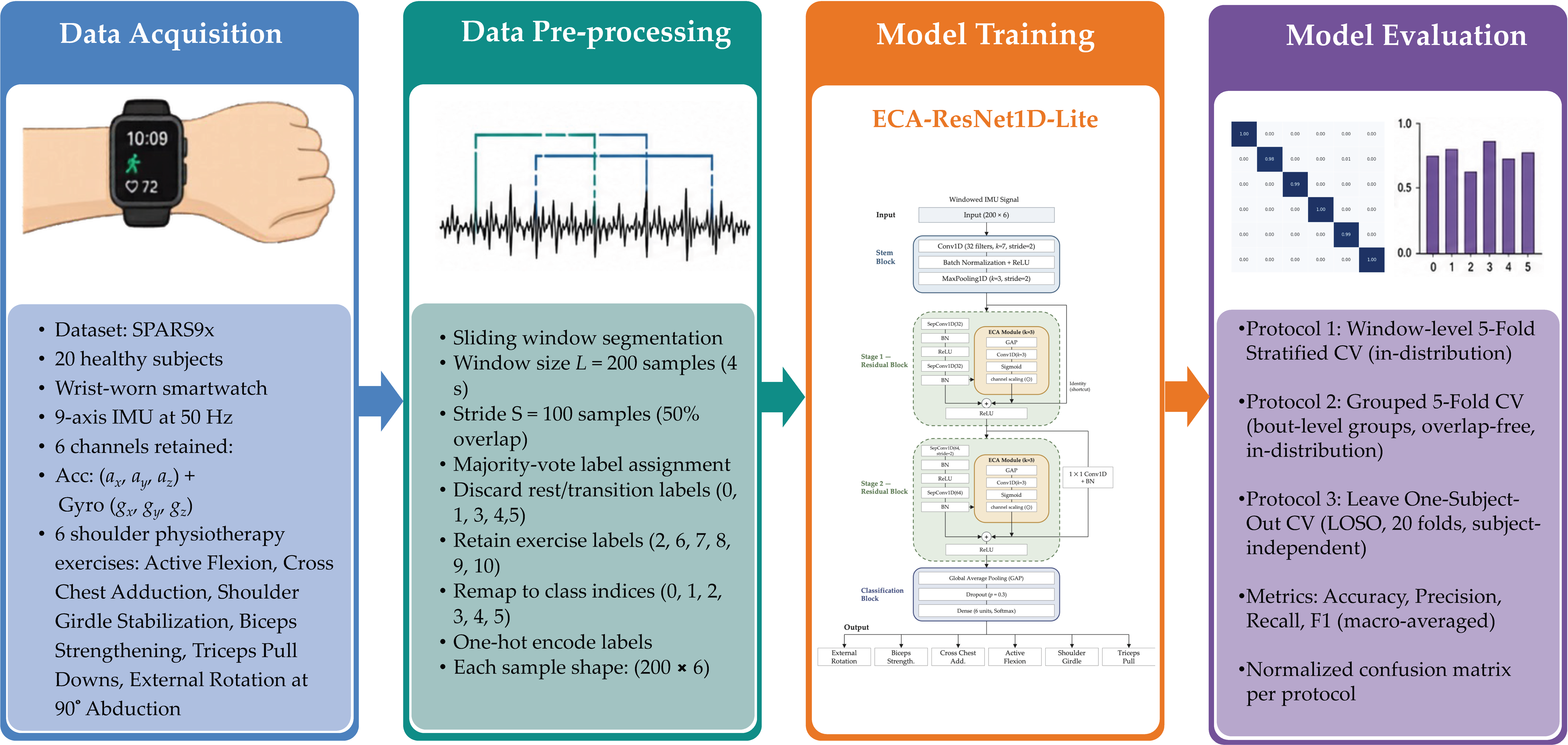
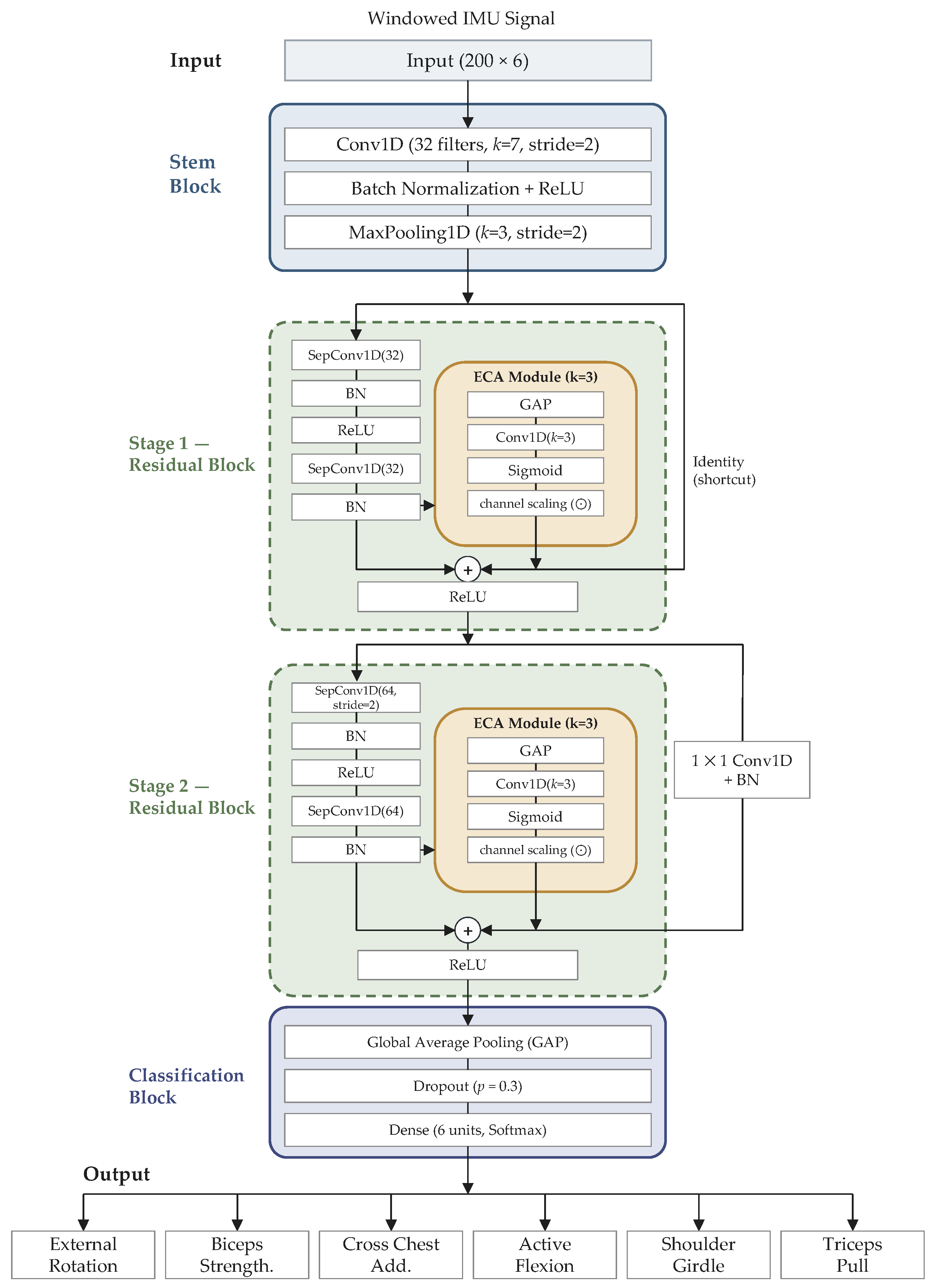
This section presents the experimental results of the proposed ECA-ResNet1D-Lite model, evaluated on the SPARS9x dataset and compared with four state-of-the-art deep learning architectures commonly used for sensor-based HAR. Two complementary evaluation protocols are used: five-fold stratified cross-validation (5-Fold CV) to assess in-distribution classification performance, and leave-one-subject-out cross-validation (LOSO CV) to measure cross-subject generalization.

4.1. Experimental Setup

All experiments were implemented in Python 3.10 using TensorFlow 2.x with the Keras high-level API and executed on Google Colab with an NVIDIA GPU accelerator. A fixed random seed of 42 was applied to both NumPy and TensorFlow to ensure reproducibility. The same training configuration was applied uniformly to all models to ensure a fair comparison: the Adam optimizer [25] with an initial learning rate of $\eta =0.001$, a mini-batch size of 256 windows, and a maximum of 200 training epochs. Two adaptive callbacks were employed: EarlyStopping (patience = 50 epochs, monitoring validation accuracy, with best-weight restoration) and ReduceLROnPlateau (reduction factor = 0.5, patience = 10 epochs). The categorical cross-entropy loss and the two evaluation protocols described in Section 3.4 were applied consistently across all models.

Baseline hyperparameters were adopted from the architectural descriptions given in the original publications and were not tuned on SPARS9x. The only modifications were those required by the input and the task: we set the classification head of every model to six units and the input layer to (200 × 6). Filter counts, kernel sizes, dilation schedules, hidden dimensions, attention-head counts, and dropout rates follow the source papers. We held the optimizer, batch size, maximum epoch count, and callback settings identical across all models. The complete layer-level configuration of every evaluated model, together with its measured parameter and multiply–accumulate counts, is given in Appendix A.

We note explicitly that an identical training protocol does not guarantee an equally well-optimized configuration for every architecture. A per-model hyperparameter search would in principle favor the recurrent and Transformer baselines, whose published settings were developed for longer sequences, more sensor channels, and larger datasets than the six-channel, 200-sample, 5276-window regime used here. Because this paper compares accuracy attainable at a given computational budget rather than the maximum attainable by each architecture, we treat the uniform protocol as the appropriate control and note the lack of per-model tuning as a limitation in Section 5.

4.2. Performance Comparison with State-of-the-Art Models

We evaluated the proposed ECA-ResNet1D-Lite against six competing architectures. Four of them are representative deep learning architectures for time-series HAR: TCN [7], DeepConvLSTM [6], InceptionTime [8], and a Transformer-based encoder [9]. These baselines cover the principal families of approaches applied to wearable sensor HAR: dilated temporal convolutions, convolutional–recurrent hybrids, multi-scale inception modules, and self-attention encoders. The remaining two, TinyHAR [21] and TinierHAR [22], are compact architectures designed under an explicit parameter-efficiency constraint and are therefore the most direct points of comparison for the present work. All competing models were trained and evaluated on SPARS9x under the same three protocols, windowing, training configuration, and random seed as the proposed model.

Table 6. Classification accuracy and model complexity on the SPARS9x dataset (the best result per column is shown in bold). Accuracy is reported to one decimal place; multiply–accumulate counts are given to three decimals because the two most efficient models differ by less than 0.05 M.

Model	Params	MACs (M)	Window 5-Fold Acc (%)	Grouped 5-Fold Acc (%)	LOSO Acc (%)
TCN [7]	88,518	17.511	99.2 ± 0.2	95.0 ± 2.8	97.5 ± 2.9
DeepConvLSTM [6]	286,598	55.279	98.8 ± 0.4	93.2 ± 2.6	96.3 ± 3.9
InceptionTime [8]	493,446	97.716	99.3 ± 0.3	96.4 ± 2.1	98.8 ± 1.4
Transformer [9]	147,526	46.772	98.4 ± 0.2	94.5 ± 2.1	96.7 ± 2.8
TinyHAR [21]	27,428	4.056	99.1 ± 0.4	97.1 ± 1.7	97.4 ± 2.5
TinierHAR [22]	7397	0.500	98.8 ± 0.3	95.4 ± 3.3	97.4 ± 2.1
ECA-ResNet1D-Lite *	13,612	0.459	99.4 ± 0.1	97.5 ± 1.9	99.1 ± 1.0

* the proposed model.

reports the model complexity and classification accuracy under all three evaluation protocols.

A caveat applies to the first four of these comparisons. TCN, DeepConvLSTM, InceptionTime, and the Transformer encoder were designed for general sequence modeling and multi-sensor activity recognition, on datasets with longer sequences, more channels, and larger activity vocabularies than SPARS9x. Parameter efficiency was not a design objective for any of them, and reporting that they use more parameters than a model designed to be small is not, by itself, meaningful. They are included because they represent the four principal architectural families applied to wearable HAR and because they establish the accuracy attainable on this dataset without a size constraint. The efficiency comparison is against models designed under the same constraint—TinyHAR and TinierHAR, introduced in Section 2.5 and evaluated here on SPARS9x under the identical protocol—and the attention ablation in Section 5.2, in which every variant shares an identical backbone.

Against the two parameter-efficient baselines, the proposed model retains an accuracy advantage under every protocol, although a narrower one than against the unconstrained architectures. TinyHAR reaches 99.1 ± 0.4% under the window-level five-fold protocol, 97.1 ± 1.7% under the grouped five-fold protocol, and 97.4 ± 2.5% under LOSO; TinierHAR reaches 98.8 ± 0.3%, 95.4 ± 3.3%, and 97.4 ± 2.1%, respectively. The efficiency comparison, however, is not one-directional, and it is worth stating precisely. TinierHAR is the smaller model by parameter count—7397 against 13,612, roughly half—yet it requires more arithmetic per window than the proposed model, 0.500 M against 0.459 M multiply–accumulate operations, because it maintains full-width feature maps for longer and adds a bidirectional recurrent stage. Parameter count and inference cost therefore do not rank the two architectures the same way. ECA-ResNet1D-Lite is the cheapest model in Table 6 to execute rather than the smallest to store, and it reaches that position without any recurrent stage, which is what makes the latency figures of Section 4.3 attainable; TinyHAR, by contrast, is both larger (27,428 parameters) and considerably more expensive (4.056 M MACs per window) than either of the other two.

As shown in Table 6, the proposed ECA-ResNet1D-Lite achieves the highest accuracy under all three evaluation protocols: 99.4 ± 0.1% under window-level 5-Fold CV, 97.5 ± 1.9% under grouped 5-Fold CV, and 99.1 ± 1.0% under LOSO CV, while requiring only 13.6K parameters—2.0×, 6.5×, 10.8×, 21.1×, and 36.3× fewer parameters than TinyHAR, TCN, Transformer, DeepConvLSTM, and InceptionTime, respectively. The consistency of the proposed model is further confirmed by the per-fold results in

Table 7. Per-fold accuracy (%) of ECA-ResNet1D-Lite under 5-fold stratified cross-validation.

Model	Fold 1	Fold 2	Fold 3	Fold 4	Fold 5	Mean ± Std
ECA-ResNet1D-Lite	99.5	99.4	99.4	99.5	99.2	99.4 ± 0.1

, which show a narrow accuracy range of 99.2–99.5% across all five folds, yielding the lowest 5-Fold standard deviation (0.1%) among all evaluated models.

Under the LOSO protocol, the performance gap between the proposed model and the baselines is more pronounced. InceptionTime records the second-highest LOSO accuracy (98.8 ± 1.4%) but at 36.3× the parameter count. TCN, DeepConvLSTM, and Transformer exhibit considerably higher LOSO standard deviations of 2.9%, 3.9%, and 2.8%, respectively, indicating inconsistent generalization across subjects—a critical limitation for deployment in real-world physiotherapy monitoring, where inter-subject variability is high. In contrast, the proposed ECA-ResNet1D-Lite achieves an LOSO standard deviation of only 1.0%, the lowest across all models, demonstrating robust and consistent cross-subject performance.

The combination of the highest accuracy, the lowest standard deviation under LOSO, and the lowest arithmetic cost of any model evaluated (0.459 M MACs per window) demonstrates that ECA-ResNet1D-Lite achieves a superior accuracy–efficiency trade-off for wrist-worn IMU-based shoulder physiotherapy exercise recognition. The ECA channel attention mechanism, adding only six parameters to the baseline lightweight residual network, enables the model to amplify exercise-discriminative channel responses and selectively suppress uninformative ones, thereby improving cross-subject generalization without sacrificing model compactness. These results confirm that ECA-ResNet1D-Lite is well suited for deployment on resource-constrained wearable devices in clinical or home-based physiotherapy monitoring scenarios.

4.3. Computational Complexity and Deployment Feasibility

Parameter count alone does not determine whether a model can run on a smartwatch. Execution time is governed by the number of arithmetic operations and by memory traffic, while feasibility is further constrained by the peak activation memory that must be resident during a forward pass and by the storage the model occupies on the device. Multiply–accumulate (MAC) operations were therefore counted by an analytic traversal of the layer graph for a batch-size-one forward pass, with floating-point operations reported as twice the MAC count; peak activation memory is the largest sum of simultaneously live tensors under a topological execution order, assuming 32-bit activations.

Table 8. Computational cost and measured on-device performance of ECA-ResNet1D-Lite.

Quantity	Value
Model complexity
Parameters (trainable/non-trainable/total)	13,036/576/13,612
Multiply–accumulate operations per window	459,072 (0.459 M)
Floating-point operations per window	0.918 M
Sustained arithmetic rate (one window per 2 s)	0.23 M MAC s−1
Peak activation memory (float32)	25.0 KiB
Model storage, TensorFlow Lite float32/int8	64.1/41.4 KiB
Model storage, Core ML float16 (deployed)	79.4 KiB
Measured on Apple Watch Ultra 2 (Apple S9 SiP, watchOS 26.6)
Latency, CPU only—mean/median/95th pct/min	0.240/0.207/0.388/0.142 ms
Latency, Neural Engine enabled—mean	0.178 ms
Duty cycle (CPU only, one window per 2 s)	0.012%
Real-time factor (CPU only)	≈8300×

reports these quantities together with latency measured on wearable hardware.

The network requires 0.459 M MAC operations per 4-s window, of which 46% occur in the second residual stage, whose pointwise convolutions operate on 64 channels, and a further 29% in the stem, the only layer applied at full temporal resolution. Peak activation memory is 25.0 KiB and occurs at the stem, where the ($100\times 32$) pre-pooling feature map and its input are simultaneously live; because the stride-2 stem and the pooling layer reduce the temporal dimension from 200 to 50 samples before any wide layer is applied, the widest stage of the network requires only 6.25 KiB. The two ECA modules together contribute six parameters and 288 MAC operations, with overheads of 0.04% and 0.06%, respectively.

To confirm that these analytic figures translate into practice, we converted the model to Core ML with float16 weights and benchmarked it on an Apple Watch Ultra 2, a current consumer smartwatch in the class targeted by this work. We verified numerical parity beforehand: across 520 probe windows, the converted model reproduced the original network’s predicted class in every case, with a maximum absolute deviation of $1.4\times {10}^{-3}$ in the softmax outputs. A single window is classified in 0.240 ms on average when Core ML is restricted to the CPU. Enabling the Neural Engine yields 0.178 ms, but the minimum latency is effectively identical across compute-unit policies (0.139–0.142 ms), and a repeat measurement on mains power produced results agreeing to within 0.002 ms; the difference is therefore attributed to scheduling variation rather than to accelerator use, and the conservative CPU-only figure is quoted throughout.

Against the 2-s interval at which windows arrive, this corresponds to a duty cycle of 0.012%, leaving the processor idle for more than 99.98% of each interval, and the deployed model occupies 79.4 KiB of storage. These measurements establish that continuous, real-time shoulder exercise recognition is computationally feasible on current smartwatch hardware without offloading to a paired smartphone. They do not establish that all-day monitoring is energy-viable, since total power draw is dominated by inertial sensor sampling, display activity, and radio use rather than by inference; a longitudinal power study under realistic duty cycles remains future work.

5. Discussion

5.1. Per-Class Performance Analysis

Table 9. Per-class precision, recall, and F1-score (%) of ECA-ResNet1D-Lite on the SPARS9x dataset (the best and worst F1-score per protocol are shown in bold and italics, respectively). Differences between protocols quoted in the text are computed from unrounded values.

Exercise Class	5F-P (%)	5F-R (%)	5F-F1 (%)	LOSO-P (%)	LOSO-R (%)	LOSO-F1 (%)
Ext. Rotation at 90° Abd.	99.6	99.4	99.5	98.3	99.2	98.6
Biceps Strengthening	98.9	99.1	99.0	98.9	97.7	98.2
Cross Chest Adduction	98.9	99.4	99.2	99.1	99.3	99.2
Active Flexion	99.4	99.2	99.3	99.3	99.4	99.3
Shoulder Girdle Stab.	98.8	98.6	98.7	98.0	95.9	96.4
Triceps Pull Downs	99.6	99.5	99.6	97.6	99.4	98.4
Macro average	99.2	99.2	99.2	98.5	98.5	98.4

presents the per-class precision, recall, and F1-score of ECA-ResNet1D-Lite for all six shoulder physiotherapy exercises under both the 5-Fold CV and LOSO CV protocols. Macro-averaged F1-scores of 99.2% (5-Fold) and 98.4% (LOSO) confirm that the model recognizes all exercise classes with high fidelity, while the 0.8 percentage-point reduction between protocols reflects the additional challenge of cross-subject generalization. The per-class breakdown reveals that recognition difficulty is not uniform across exercise types, and that the drop from 5-Fold to LOSO varies substantially by class—a pattern that the biomechanical distinctiveness and inter-subject variability of each exercise can explain.

Triceps Pull Downs achieves the highest 5-Fold F1-score (99.6%), followed by External Rotation at 90° Abduction (99.5%) and Active Flexion (99.3%). Under LOSO, Active Flexion records the best F1-score across all classes (99.3%), with Cross Chest Adduction a close second (99.2%). The strong recognition of Triceps Pull Downs under 5-Fold CV is attributable to its highly distinctive downward elbow-extension motion: the wrist-mounted accelerometer captures a consistent low-to-high axial deceleration signature as the forearm descends, producing a temporally compact and subject-invariant pattern. Similarly, Active Flexion—which involves raising the arm forward in the sagittal plane—generates a clean, monotonic acceleration arc along the anterior axis that is reliably detected across unseen subjects, explaining its strong LOSO retention (99.3%). Cross Chest Adduction, involving horizontal arm movement in the transverse plane, produces a laterally dominant acceleration pattern that contrasts sharply with all other exercises, enabling consistent recognition even when subject-specific amplitude and velocity vary.

Shoulder Girdle Stabilization presents the greatest recognition challenge across both protocols, recording the lowest F1-scores of 98.7% (5-Fold) and 96.4% (LOSO). Its LOSO recall of 95.9% is the lowest among classes in this study, indicating a notably higher rate of false negatives when generalizing to unseen subjects. This is consistent with the biomechanical nature of the exercise. Unlike the other five exercises, Shoulder Girdle Stabilization requires the subject to maintain a quasi-static isometric contraction of the scapular retractors and depressors against band resistance, with limited gross arm movement. The resulting IMU signal is characterized by low-amplitude fluctuations in all three accelerometer and gyroscope axes, with a temporal profile that varies considerably between subjects depending on posture, grip tightness, and the degree of compensatory trunk movement. This high inter-subject variability in a low-discriminability signal space explains both the absolute performance deficit and the larger 5-Fold-to-LOSO drop ($-2.3$ percentage points) observed for this class.

The largest reductions in F1-score between the 5-Fold and LOSO protocols are observed for Shoulder Girdle Stabilization ($-2.3$ pp), Triceps Pull Downs ($-1.2$ pp), and External Rotation at 90° Abduction ($-0.8$ pp); these differences are computed from unrounded values. For Triceps Pull Downs, LOSO precision falls to 97.6%. At the same time, recall remains high (99.4%), suggesting that window segments from other exercise classes are occasionally classified as Triceps Pull Downs in unseen subjects—possibly owing to inter-subject variation in the speed and range of elbow extension, which can produce downward acceleration profiles that partially resemble those of Active Flexion or Biceps Strengthening in certain individuals. Biceps Strengthening similarly exhibits a LOSO recall decrease to 97.7%, reflecting that the model occasionally misses Biceps instances in new subjects, likely because the elbow-flexion trajectory of a curl—involving upward wrist acceleration—overlaps kinematically with the ascending phase of Active Flexion when subjects deviate from standard form.

Active Flexion and Cross Chest Adduction maintain near-identical F1-scores between 5-Fold and LOSO (Active Flexion: 99.3% and 99.3%; Cross Chest Adduction: 99.2% and 99.2%; both unchanged at one decimal place), demonstrating that the motion patterns associated with these exercises are highly stable across subjects. This cross-subject stability is notable because it implies that the learned feature representations for these two classes capture intrinsic exercise kinematics rather than subject-specific movement styles. The ECA channel attention mechanism likely contributes to this generalization. By selectively weighting the most informative accelerometer and gyroscope channels for each exercise, the model suppresses subject-dependent nuisance variations in less discriminative channels and focuses on the exercise-defining axes of motion.

Under LOSO—the most demanding evaluation protocol—all classes except Shoulder Girdle Stabilization achieve per-class F1-scores of at least 98.2%, demonstrating clinically relevant recognition accuracy for each shoulder physiotherapy exercise. The only class falling below 97% recall under LOSO (Shoulder Girdle Stabilization, 95.9%) is the exercise with the most ambiguous IMU signature by design. These results suggest that future work should consider supplementary sensing modalities—such as surface electromyography or additional IMU placement proximal to the scapula—to better capture the subtle muscular activation patterns of stabilization exercises in a subject-independent manner.

5.2. Ablation Study: Attention Mechanism Integration

To isolate the contribution of the channel attention mechanism to the overall performance of ECA-ResNet1D-Lite, an ablation study was conducted in which four attention variants—SE [11], ECA [12], CBAM [26], and MHSA [27]—were each integrated into the ResNet1D-Lite backbone under identical training conditions. SE, ECA, and CBAM were inserted within each residual block before the shortcut addition, following canonical SE-ResNet and ECA-ResNet placement. MHSA was applied after each residual stage to operate over the full temporal sequence.

Table 10. Ablation study results for attention mechanism integration into ResNet1D-Lite on the SPARS9x dataset (ΔP: additional parameters relative to the baseline; best result per column in bold and worst in italics). Accuracy differences quoted in the text are computed from unrounded values.

Model	Params	ΔP	5-Fold Acc (%)	LOSO Acc (%)
ResNet1D-Lite (Baseline)	13.6 K	—	99.6 ± 0.1	98.9 ± 1.4
+SE	16.2 K	+2560	99.5 ± 0.2	99.0 ± 1.2
+CBAM	16.2 K	+2588	99.5 ± 0.3	98.4 ± 2.4
+MHSA	26.0 K	+12,368	98.9 ± 0.3	98.5 ± 1.4
+ECA (proposed)	13.6 K	+6	99.4 ± 0.1	99.1 ± 1.0

and

Table 11. Per-fold accuracy (%) of each attention variant under 5-fold stratified CV.

Model	Fold 1	Fold 2	Fold 3	Fold 4	Fold 5	Mean ± Std
Baseline	99.6	99.7	99.6	99.5	99.3	99.6 ± 0.1
+SE	99.6	99.6	99.6	99.5	99.2	99.5 ± 0.2
+CBAM	99.3	100.0	99.3	99.5	99.1	99.5 ± 0.3
+MHSA	99.0	99.1	98.9	99.2	98.4	98.9 ± 0.3
+ECA (proposed)	99.5	99.4	99.4	99.5	99.2	99.4 ± 0.1

summarize the results.

ECA-ResNet1D-Lite achieves the highest LOSO accuracy of 99.1 ± 1.0%—improving upon the non-augmented baseline by 0.2 percentage points—while introducing only six additional parameters, representing a parameter overhead of 0.04% relative to the 13.6 K baseline. This marginal cost arises from a single 1D convolution of kernel size k = 3 applied per ECA module (two modules in total, one per residual stage). The LOSO standard deviation simultaneously decreases from 1.4% (baseline) to 1.0%, the lowest recorded across all five variants. This dual improvement—higher mean accuracy and lower variance under subject-independent evaluation—provides strong evidence that ECA’s local inter-channel interaction selectively reinforces exercise-discriminative IMU channels in a subject-agnostic manner. Under 5-Fold CV, ECA records the lowest fold-to-fold standard deviation (0.1%), confirming the most stable in-distribution performance despite having a marginally lower 5-Fold mean (99.4%) than the baseline (99.6%). This pattern is consistent with the known regularization effect of channel attention. By suppressing uninformative channels, ECA reduces overreliance on subject-specific signal characteristics present in the training data but absent in unseen subjects.

The SE variant yields a negligible LOSO improvement over the baseline ($\mathsf{\Delta }$ = +0.01 pp computed before rounding; the two means round to 99.0% and 98.9%, respectively, in Table 10) while adding 2560 parameters (+18.8%). The SE module employs a fully connected bottleneck that compresses the C-dimensional channel descriptor to $C/r=C/4$ and re-expands it, introducing a dimensionality-reduction step that has been shown to discard inter-channel correlations relevant to fine-grained signal recalibration. In the context of IMU-based HAR, where the six input channels carry complementary yet tightly coupled motion information (accelerometer and gyroscope axes), this information bottleneck may limit the effectiveness of channel recalibration compared with ECA’s dimension-preserving approach. The SE variant does reduce the LOSO standard deviation compared with the baseline (1.2% vs. 1.4%), but this improvement is substantially smaller than that achieved by ECA (1.0%) at a 427× greater parameter overhead.

CBAM underperforms all other variants under LOSO (98.4 ± 2.4%), recording both the lowest LOSO mean and the highest LOSO standard deviation across the ablation. The 2.4% LOSO standard deviation—approximately 2.5× larger than that of ECA—indicates highly inconsistent cross-subject generalization, suggesting that CBAM’s spatial attention pathway introduces sensitivity to subject-specific temporal patterns rather than universally discriminative ones. CBAM applies a seven-sample 1D convolutional spatial attention map that reweights time steps based on the combination of average- and max-pooled channel features; for short (200-sample) wrist IMU windows, this temporal gating may overfit to within-subject exercise pacing and rhythm, which vary considerably between individuals. Under 5-Fold CV, CBAM exhibits the highest fold-to-fold variance (±0.3%), further reflecting its training instability. Notably, Fold 2 achieves 100.0% accuracy while Fold 5 drops to 99.1%, a spread of 1.0 percentage points (0.95 pp before rounding)—the largest among all variants—indicative of overfitting to specific data partitions.

MHSA yields the weakest overall performance: 98.9 ± 0.3% under 5-Fold CV and 98.5 ± 1.4% under LOSO, while requiring 26.0K parameters—the largest model in the ablation study and a 91% increase over the baseline. MHSA was placed after each residual stage to enable global temporal modeling over the full feature sequence. However, self-attention mechanisms are architecturally designed for long sequences with complex long-range dependencies (e.g., natural language or vision tokens), and their quadratic complexity with respect to sequence length yields diminishing returns for the comparatively short 50-sample and 25-sample feature maps produced by Stage 1 and Stage 2 of ResNet1D-Lite, respectively. Furthermore, the learnable query–key–value projections of MHSA introduce a large number of additional parameters that are at risk of overfitting to subject-specific temporal patterns under the limited per-subject data available in LOSO training sets.

Ranking the five variants by LOSO accuracy per unit of additional parameter overhead reveals a decisive advantage for ECA: a gain of 0.2 percentage points for 6 additional parameters, compared with $+0.01$ pp for 2560 parameters (SE), $-0.5$ pp for 2588 parameters (CBAM), and $-0.4$ pp for 12,368 parameters (MHSA); these differences are computed from unrounded values. This analysis confirms that ECA’s design philosophy—capturing local cross-channel interactions via a compact 1D convolution without dimensionality reduction—is uniquely well suited to the low-channel, short-window IMU setting of wearable physiotherapy monitoring. The results collectively support selecting ECA as the attention mechanism of choice for ECA-ResNet1D-Lite and demonstrate that neither increasing model capacity via SE or CBAM nor introducing global temporal reasoning via MHSA provides benefits commensurate with the additional computational cost for this task and dataset.

5.3. Exercise Identity Versus Subject Identity

The results of Section 4.2 rest on an implicit assumption: that the information distinguishing one exercise from another can be separated from the information distinguishing one person from another. Research on biometric style modeling suggests this separation is neither automatic nor complete. Huang et al. [28] show that a writer’s identity remains recoverable from handwriting even when the written content changes entirely, by abstracting style from content through dedicated channel- and trajectory-attention pathways. Their objective is the mirror image of the one pursued here: they suppress content to expose person-specific style, whereas this work suppresses person-specific style to expose exercise content. The comparison is instructive because the mechanism is shared—a channel attention pathway of the same family as the ECA module used here proves sufficient to isolate identity, suggesting that such modules do not remove person-specific information so much as reweight it.

The present results are consistent with that reading, though in a form worth stating precisely. Moving from the grouped protocol, in which folds are formed at recording level, to LOSO evaluation does not lower mean accuracy (97.5 ± 1.9% and 99.1 ± 1.0%, respectively; the two protocols differ in fold structure and in the amount of training data available per fold, and they are not directly paired), so subject identity is not, on this dataset, an obstacle to average recognition. Instead, its trace is visible in where the cross-subject cost falls. The macro F1-score declines from 99.2% under window-level five-fold evaluation to 98.4% under LOSO. That decline is unevenly distributed: Shoulder Girdle Stabilization loses 2.3 percentage points and Triceps Pull Downs 1.2, while Active Flexion and Cross Chest Adduction are unchanged at one decimal place (99.3% and 99.2% under both protocols). Residual dependence on the individual therefore concentrates in the classes whose signature is quasi-static or kinematically ambiguous rather than spreading evenly across the exercise vocabulary, and the standard deviation of 1.0% across the 20 held-out subjects—the lowest in Table 6, but not zero—indicates that how well the model transfers still varies from person to person. Channel recalibration is at best a weak, unsupervised form of the separation in question, since ECA reweights channels according to their global response and is never trained to be invariant to who is moving. Methods that address the residual dependence explicitly—subject-adversarial training, or content–style disentanglement in which an auxiliary objective penalizes recoverable subject information [28,29]—would target it directly.

A dataset-level limitation follows. SPARS9x provides exercise labels but no demographic, clinical, or movement-quality annotation, so the sources of the between-subject dispersion reported above cannot be attributed. Benchmark design in adjacent fields has moved toward finer person-level annotation: PersoMoni [30], for example, annotates fifteen validated trait dimensions rather than a coarse label set, permitting analysis of which person-level factors drive model behavior rather than merely establishing that such factors exist.

6. Conclusions and Future Directions

This paper presented ECA-ResNet1D-Lite, a lightweight one-dimensional residual network augmented with ECA, for recognizing six shoulder physiotherapy exercises from wrist-worn IMU data on the SPARS9x dataset. Under window-level five-fold stratified cross-validation, the proposed model achieved a classification accuracy of 99.4 ± 0.1%, and under the more stringent LOSO protocol—the standard benchmark for subject-independent wearable HAR—it attained 99.1 ± 1.0%, with the lowest cross-subject standard deviation (1.0%) among all evaluated models. These results surpass all six baseline architectures (TCN, DeepConvLSTM, InceptionTime, a Transformer encoder, TinyHAR, and TinierHAR) while requiring only 13,612 parameters and 0.459 M multiply–accumulate operations per window—up to 36.3× and 213× fewer, respectively, than the unconstrained baselines, and the lowest arithmetic cost of any model evaluated—demonstrating a superior accuracy–efficiency trade-off for deployment on resource-constrained wearable devices.

An ablation study comparing four attention variants (SE, ECA, CBAM, and MHSA) confirmed that ECA provides the best balance between representational power and computational cost among the variants evaluated. ECA achieved the best LOSO accuracy (99.1 ± 1.0%) while adding only six parameters—a 0.04% overhead relative to the baseline. SE offered no material LOSO improvement at the cost of 2560 additional parameters; CBAM degraded LOSO performance by 0.5 pp, with its spatial attention branch overfitting to subject-specific exercise pacing; and MHSA yielded the weakest overall results owing to quadratic complexity limitations on the short 50- and 25-sample temporal feature maps produced by the network. These findings support ECA as a well-suited attention mechanism for compact wearable HAR models.

Per-class analysis showed that five of the six exercise classes achieved LOSO F1-scores of at least 98.2%, with Active Flexion (99.3%) and Cross Chest Adduction (99.2%) exhibiting near-perfect, highly stable recognition on unseen subjects. Shoulder Girdle Stabilization remained the most challenging class (LOSO F1-score: 96.4%; LOSO recall: 95.9%), a result consistent with its quasi-static, low-amplitude IMU signature and high inter-subject postural variability—an inherent limitation of single-site wrist-mounted sensing for isometric exercises.

Several directions for future work are identified. First, supplementary sensing modalities—such as surface electromyography or an additional IMU placed proximal to the scapula—should be investigated to better capture the subtle muscular activation patterns of stabilization exercises in a subject-independent manner. Second, evaluation in larger, more clinically diverse cohorts, encompassing patients with shoulder pathologies across age groups, would strengthen the generalizability of the findings. Third, while Section 4.3 establishes that inference is computationally feasible on a commercial smartwatch, it does not establish energy viability; a longitudinal power-consumption study under realistic sensor duty cycles is required before claiming continuous all-day monitoring. Fourth, the between-subject dispersion reported in Section 5.3 motivates explicit invariance methods. Subject-adversarial training and content–style disentanglement, which have proven effective where person-specific style must be separated from task content [28,29], would target this dependence directly rather than relying on the incidental regularization provided by channel attention. Fifth, progress on subject independence is limited by what current rehabilitation benchmarks annotate. Datasets that record demographic attributes, impairment severity, execution quality, and compensatory movement patterns alongside exercise labels [30] would allow researchers to attribute sources of between-subject variation rather than merely observe them. Finally, extending the framework to longitudinal home-based physiotherapy monitoring—including exercise adherence tracking and movement quality scoring—represents a clinically meaningful avenue that could directly support remote rehabilitation programs.