Stable Discrimination Can Hide Reliability Failures in AI Decision Support Under Distribution Shift and Changing Target Definitions

Abstract

Stable discrimination can coexist with unreliable probabilities, abstention policies, and uncertainty sets under distribution shift. We evaluate this mismatch with CRIT-AID, an executable multi-domain reliability-audit framework that separates model fitting, probability calibration, operating-rule calibration, and testing and then transports source-derived rules unchanged to target domains. Across four public tabular domains, stable discrimination did not imply stable probability quality, selective operating points, or conformal uncertainty. On identical ACS 2024 records, changing the income target definition left AUROC nearly unchanged, while ECE differed by 0.083; prevalence-intercept alignment reduced this difference to −0.004, showing that target semantics can alter probability reliability without materially changing ranking. Across 27 primary 90% conformal conditions, label-conditional calibration improved worst-class coverage in 18 but worsened it in 9 and usually increased prediction-set size. LightGBM sensitivity changed absolute discrimination without removing the mismatch among reliability dimensions. These findings show that discrimination alone is insufficient evidence for reliable AI decision support: audits should test the transportability of probability mappings, operating rules, class-specific validity, and uncertainty informativeness when deployment conditions or target meanings change.

1. Introduction

Artificial intelligence (AI) decision support is increasingly evaluated in settings where a single performance score is an inadequate description of operational reliability. A deployed system may rank cases, output probabilities, trigger escalation, abstain, or return a prediction set. These outputs can fail differently under temporal, geographic, institutional, population, or measurement change. Reliability therefore concerns not only discrimination but also target meaning, probability quality, the transport of operating rules, and the validity and informativeness of uncertainty outputs. This broader view is consistent with risk-management approaches that treat validity and reliability as context-dependent properties that require measurement and monitoring [1].

In this article, reliability failure is used at the statistical-property level: a transported probability quantity, operating rule, or uncertainty output fails to preserve the source-domain property it is intended to represent. The term does not by itself denote an application-level pass/fail judgment, safety failure, clinical harm, or governance failure; those interpretations require domain-specific tolerances and downstream evidence.

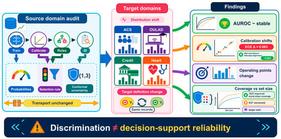
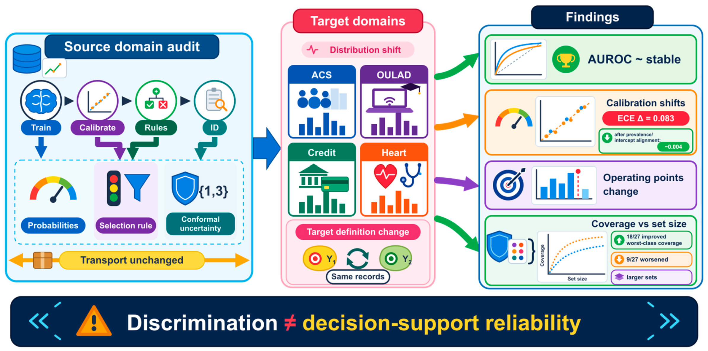
Stable discrimination and decision-support reliability are not interchangeable. AUROC can remain comparatively stable while prevalence, calibration intercept, proper scores, class-specific uncertainty, or the achieved operating point of a source-calibrated threshold changes. Conversely, a marginal uncertainty metric can appear acceptable while one outcome class is systematically undercovered. A model can therefore look almost unchanged by AUROC while becoming less reliable for decisions built on its probabilities, abstention rules, or uncertainty outputs. For consequential use, the relevant question is not only whether a model still discriminates but whether the quantities and rules built around its predictions retain the statistical meaning assumed by the deployment process.

Naturally occurring distribution shift is now a standard evaluation problem. WILDS, TableShift, Shifts, and Wild-Time provide benchmarks spanning temporal, geographic, institutional, and population change [2,3,4,5]. Folktables supports comparable ACS tasks across years and states [6]. The broader dataset-shift literature distinguishes covariate, label, and concept changes and cautions against treating them as one mechanism [7]. Distribution shift can change not only the distribution of inputs and outcomes but also the operational meaning of the prediction target itself. A nominal income threshold, diagnostic criterion, policy trigger, or eligibility rule can preserve a familiar label name while changing which cases count as positive. A model can therefore preserve discrimination while the probabilities and decisions attached to that ranking cease to represent the same operational quantities.

Probability calibration, selective prediction, and conformal prediction address complementary parts of this reliability problem. Calibration evaluates correspondence between probabilities and observed event rates and is supplemented by proper scores [8,9,10,11,12,13]. Selective prediction evaluates which cases are accepted at a confidence threshold and the risk among accepted cases [14,15]. Split-conformal classification offers finite-sample marginal coverage under exchangeability [16,17], but ordinary guarantees need not transport under shift [18,19,20]; marginal coverage can also conceal class-specific undercoverage or be achieved with uninformative sets.

Technical reliability is necessary but not sufficient for appropriate human reliance. Human–AI studies show that erroneous recommendations may still be followed and that explanations do not automatically prevent overreliance [21]. CRIT-AID therefore does not equate a passed technical audit with trustworthy human use. Instead, it defines a reproducible technical evidence layer that can be connected to later human-factors evaluation.

In this article, CRIT-AID denotes the overall empirical reliability-audit framework: its conceptual scope, required reliability dimensions, stress-test logic, common result interface, and reproducibility artifacts. The term CRIT-AID protocol is reserved for the mandatory seven-step operational procedure used to execute that framework. Neither term denotes a predictive model. This distinction is maintained throughout this revised manuscript.

The contribution is therefore not a new classifier, calibration algorithm, or conformal method. Its novelty lies in a reproducible data-partition, transport, stress-test, and reporting contract: model fitting, probability calibration, selection/conformal calibration, and testing are separated; source-derived operating rules are transported unchanged; target definitions can be varied on identical records; equal-budget evidence degradation distinguishes amount from informational relevance; and marginal reliability is reported together with class-specific and informativeness diagnostics. The individual statistical tools are established. The protocol contribution is not that AUROC, calibration, selective prediction, and conformal prediction are merely listed together; it is that they become outputs of the same source-to-target transport experiment under one pre-declared estimand. This common transport contract prevents a favorable discrimination metric from standing in for the decision-relevant quantities that the deployed system actually uses.

Four research questions were pre-specified. RQ1 asks how source-ID and target-OOD discrimination, probability quality, calibration, selective prediction, and conformal prediction differ. RQ2 asks whether equal-budget removal of decision-relevant features is more damaging than random removal. RQ3 asks whether source-fitted probability mappings, selection thresholds, and conformal quantiles preserve their intended operating properties in target domains and outcome classes. RQ4 asks how strongly an apparent temporal reliability difference depends on target definition, OULAD module/presentation composition, landmark estimand, or evidence-availability assumptions.

2. Related Work and Research Gap

2.1. Distribution Shift and Reliability Evaluation

Distribution shift occurs when deployment data differ from development data [7]. WILDS, TableShift, Shifts, and Wild-Time standardize naturally occurring shift evaluation [2,3,4,5]. These resources make source–target generalization measurable, but they are primarily model/benchmark infrastructures rather than prescriptive audits of probability calibration, abstention operating points, target semantics, and conformal informativeness. CRIT-AID uses the benchmark logic of fixed source and target domains while making these downstream decision-support quantities mandatory outputs. Group-robust and cost-sensitive learning address adjacent objectives, namely worst-group generalization and application-specific asymmetric error costs, rather than the same audit question [22,23].

Tabular model choice is also relevant to external validity. Tree ensembles remain strong reference models for typical medium-sized tabular tasks, and their inductive biases differ materially from linear and neural models [24]. Recent work on vision and language foundation models likewise treats calibration, selective prediction, and shift detection as distinct reliability objectives rather than consequences of average predictive performance [25]. Accordingly, logistic regression is used here as a low-capacity primary audit probe rather than as a claim about the best tabular architecture, and a fixed LightGBM specification is used to test whether the principal reliability patterns depend on that choice.

2.2. Calibration and Target Semantics

Post hoc probability calibration is well established [9,10,12,13]. Source-domain calibration improvements need not persist after shift [26], ECE depends on binning and finite-sample behavior [27], and label-shift calibration methods show that the assumed shift mechanism matters [28]. A separate issue arises when the operational definition of Y changes. A nominal income threshold, diagnostic criterion, policy trigger, or eligibility rule can preserve a familiar label name while changing which records are positive. The ACS experiment therefore keeps the records fixed while changing the target construction, allowing target semantics to be audited without conflating them with a different target sample.

2.3. Selective and Conformal Uncertainty Outputs

Selective prediction trades coverage/selection against conditional error [14,15]. Split conformal prediction supplies marginal coverage under exchangeability [16,17], while weighted, unlabeled-target, and generalized-shift methods address particular departures from exchangeability under additional assumptions [18,19,20,29]. Recent conformal work also emphasizes that class-conditional or covariate-conditional coverage is not the end of the conditional-validity problem [30]. Marginal and label-conditional conformal calibration solve different finite-sample objectives. Class conditioning may improve the worst-covered class, but its smaller class-specific calibration samples can produce coarser quantiles, larger sets, and, under shift, no universal improvement. Shift-aware methods attempt to repair uncertainty under specified assumptions; CRIT-AID asks a complementary transport question: whether a source-defined uncertainty procedure remains reliable when carried to the target without target-test tuning. Reliability therefore requires joint reporting of class-specific coverage and informativeness rather than a binary “conformal/non-conformal” label.

2.4. Relation to Existing Audit and Reporting Frameworks

CRIT-AID is complementary to governance, documentation, production-readiness, and benchmark frameworks. The NIST AI Risk Management Framework provides broad risk-management functions and explicitly places measurement and monitoring within a socio-technical context [1]. Model Cards standardize documentation of intended use and performance across relevant groups and conditions [31]. The ML Test Score organizes production-readiness tests and monitoring needs [32]. WILDS and TableShift standardize naturally occurring distribution-shift benchmarks [2,3].

Table 1. Scope comparison with adjacent audit, reporting, production-readiness, and distribution-shift frameworks. “Required” means the item is part of the CRIT-AID execution contract; “contextual” means the framework can accommodate it without prescribing the same empirical operation. The comparison is functional, not a quality ranking.

Framework	Primary Role	Explicit Source–Target Shift	Separate Probability-Calibration Transport	Target-Definition Sensitivity	Transported Selection/Conformal Rules	Governance/Human Scope
NIST AI RMF [1]	Risk-management framework	Contextual	Contextual	Contextual	Contextual	Broad
Model Cards [31]	Model documentation/reporting	Contextual	Not prescribed	Intended-use context	Not prescribed	Broad transparency
ML Test Score [32]	Production readiness/testing	Training–serving and monitoring focus	Not prescribed	Not prescribed	Not prescribed	Process/operations
WILDS/TableShift [2,3]	Shift benchmarking	Core	Not core	Not core	Not core	Not core
CRIT-AID	Executable technical reliability audit	Required	Required	Required where definitional alternatives exist	Required	Interface only

therefore compares scope rather than assigning a scalar “winner” to frameworks designed for different purposes.

The research gap is consequently not the absence of AUROC, calibration, abstention, conformal prediction, stress testing, or documentation in isolation. It is the absence of a compact executable protocol that forces these quantities to share the same target estimand, disjoint calibration/test structure, source-to-target transport rule, and machine-readable reporting surface. Within this narrower technical-audit scope, three distinguishing strengths follow. First, reliability dimensions are evaluated on one pre-declared estimand rather than in separate best-case analyses. Second, source-derived probability mappings, selection thresholds, and conformal rules are transported unchanged while target semantics or evidence conditions are deliberately stressed, making transportability itself an observable audit object. Third, deterministic cohort/split manifests and machine-readable outputs preserve an inspectable audit trail. This design also makes negative evidence reportable: a method that improves one reliability dimension but worsens another remains visible rather than being absorbed into a single score.

3. Materials and Methods

3.1. Operational Definition of the CRIT-AID Protocol

The CRIT-AID protocol is a seven-stage empirical procedure for testing whether a probabilistic AI decision-support pipeline preserves specified reliability properties when a source-defined estimand, probability mapping, operating rule, or evidence structure is transported to a target domain or controlled stress condition. A conforming execution prohibits target-test tuning, preserves disjoint fitting/calibration/test roles, and reports discrimination, probability quality, selective behavior, conformal validity, and informativeness through one common result interface. CRIT-AID is the broader framework containing this protocol together with the stress-test specifications, metric interface, interpretation rules, and reproducibility artifacts.

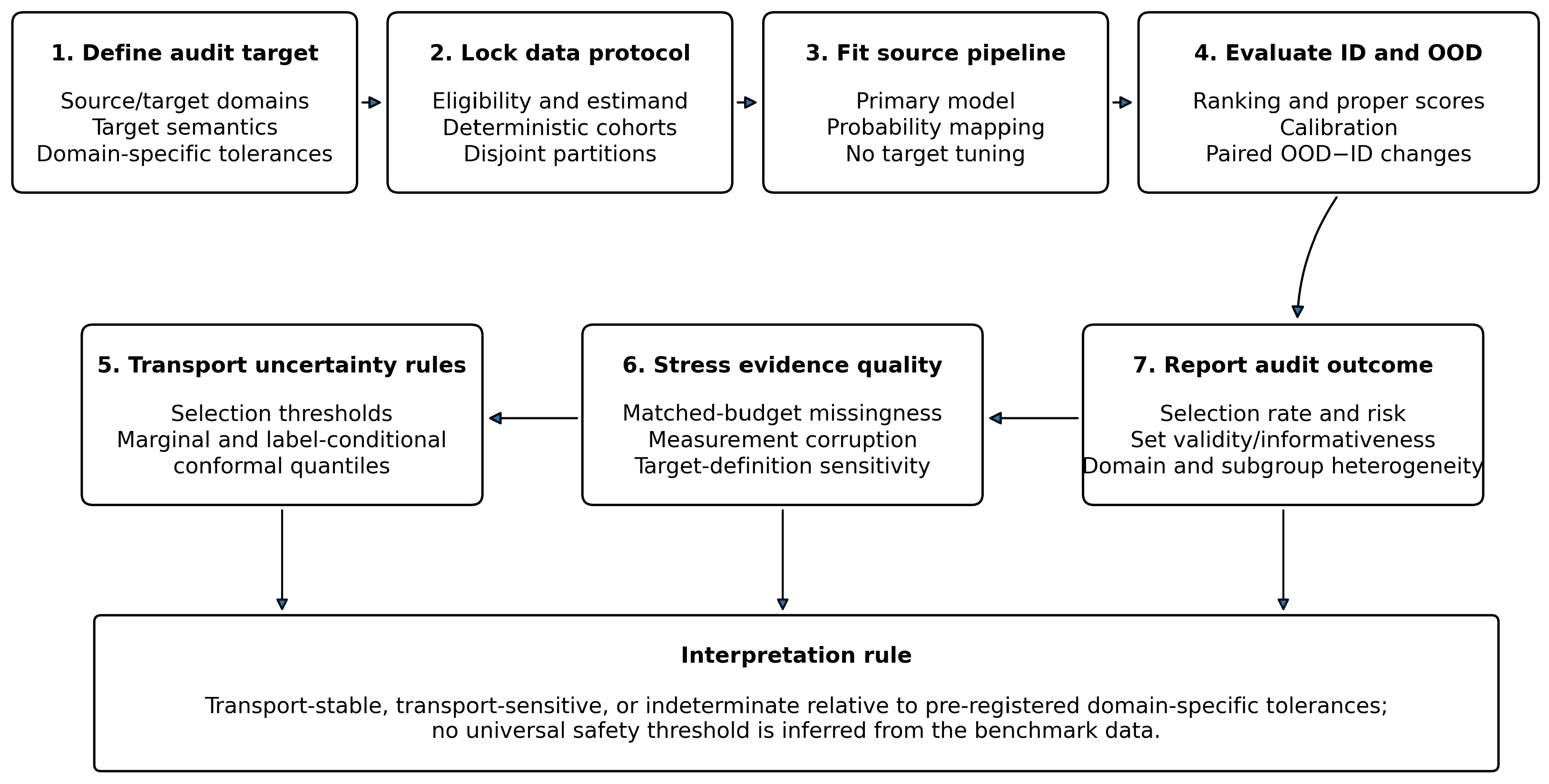
The CRIT-AID protocol receives a source domain, a target domain or controlled stress condition, a documented target variable, a probabilistic binary classifier, and domain-specific tolerances supplied before target evaluation. The mandatory workflow is shown in Figure 1. First, the target estimand, eligibility rule, source/target domains, and evidence-availability time are fixed. Second, deterministic cohorts and four disjoint source partitions are created. Third, a primary predictive pipeline and probability mapping are fitted without target tuning. Fourth, the same metrics are evaluated on source ID-test and target OOD-test data and paired OOD-minus-ID changes are calculated. Fifth, selection thresholds and conformal quantiles estimated in the source domain are transferred unchanged. Sixth, target semantics and matched-budget evidence degradation are audited where applicable. Seventh, domain, class, and subgroup heterogeneity are reported.

The protocol does not impose a universal safety threshold. For deployment use, the auditor must pre-register domain-specific tolerances ${\delta }_m$ for each metric or operating property. A result is classified as transport-sensitive when the paired target change exceeds its tolerance, transport-stable when it remains within tolerance, and indeterminate when the uncertainty range crosses the tolerance boundary. The present study reports empirical changes and variability without assigning application-specific pass/fail status. Throughout this manuscript, the phrase reliability failure therefore refers to loss of preservation of a stated statistical reliability property under transport or stress; it is not itself an application-level safety classification.

The primary endpoints were AUROC, Brier score, ECE, achieved selection rate and selective risk at a source-calibrated desired selection rate of 0.80, and empirical 90% marginal and label-conditional conformal coverage with average set size and singleton rate. Secondary endpoints were average precision (AP), PR skill, log loss, calibration intercept and slope, high-confidence error proportion (HCEP) at 0.80, 0.90, and 0.95, complete risk–selection curves, area under that curve (AURC), excess AURC, selection rates of 0.50, 0.70, 0.90, and 0.95, and conformal levels of 0.95 and 0.80. Complete machine-readable results for every declared combination are contained in the versioned reproducibility archive.

3.2. Analysis Matrix and Post Hoc Robustness Analyses

Table 2. Analysis matrix. LR: logistic regression; LC: label conditional. The final four rows are explicitly post hoc.

Analysis	Status	Model/Method	Mapping	Repetitions and Role
ACS target definitions	Primary	LR; marginal/LC	Platt	10 split refits; 5 independent computational cohorts
ACS model/mapping grid	Secondary	LR, LightGBM	Raw, Platt, isotonic	10 split refits; mapping sensitivity
OULAD exact-pair transfer	Primary	LR; marginal/LC	Platt	10 refits per pair and horizon
OULAD estimand/score sensitivity	Secondary	LR fixed effects	Platt	10 pooled refits per specification
Credit evidence degradation	Primary	LR; marginal/LC	Platt	20 refits; 20 random feature sets per refit
Heart site transfer	Primary	LR, no indicators	Platt	10 refits per held-out site
Heart missingness sensitivity	Secondary	LR with indicators	Raw, Platt, isotonic	10 refits per held-out site
ACS same-record metric decomposition	Post hoc	Fixed LR pipelines	Platt	75,000 target records; 300 stratified bootstraps for prevalence-aligned residuals
Cross-domain LC-vs-marginal comparison	Post hoc	Primary LR analyses	Platt	27 conditions; 290 repeated paired comparisons
Cross-domain model-family sensitivity	Post hoc	LR, LightGBM	Platt	Fixed LightGBM configuration in all four domains; no target tuning
Variance-component integration	Post hoc	Mixed-effects models	–	OOD-minus-ID changes; domain, condition, and refit components

distinguishes pre-specified primary/secondary analyses from post hoc robustness analyses added to interrogate target-definition, conformal-method, model-family, and cross-domain variability. Post hoc analyses were not used to redefine the primary estimands or select favorable target results.

3.3. Datasets, Cohort Formation, and Identifiers

Four public tabular datasets represented distinct decision-support contexts. They were methodological test beds rather than evidence of operational readiness. The temporal analyses were dataset-specific and independent. ACSIncome used the 2018 and 2024 ACS 1-Year PUMS person files for California, Florida, New York, and Texas [33,34]. OULAD used the Open University Learning Analytics Dataset public release [35,36], containing internal 2013B/J and 2014B/J module-presentation codes. The 2018 and 2024 files were ACS files and did not add further OULAD years.

Stable record keys were created before sampling. ACS keys combined year, state, SERIALNO, and SPORDER; OULAD keys combined module, presentation, student identifier, and horizon; credit records retained original row order; Heart Disease keys combined site and site-specific row number. The archive contains raw-file SHA-256 checksums, cohort manifests, split assignments, seed lists, feature dictionaries, and harmonization tables. Raw public datasets are not redistributed.

Table 3. Source data, eligible data, and computational cohorts.

Dataset	Public Source Content	Prepared or Computational Cohort	Primary Shift/Stress Design
ACSIncome	2018 and 2024 ACS 1-Year PUMS person files for California, Florida, New York, and Texas [33,34]	1,097,452 eligible records; deterministic 100,000-source and 75,000-target cohorts	2018 to 2024 temporal transfer and target-definition sensitivity
OULAD	32,593 registrations, 22 module presentations, 10,655,280 daily VLE summaries [35,36]	130,372 registration–horizon candidates over four horizons; primary analyses use days 14 and 56 and nine exact pairs	Within-release 2013 to 2014 matched module–period transfer
South German Credit	1000 cases and 20 predictors [37,38]	600/150/100/150 train/probability-calibration/selection-conformal/ID-test observations per refit	Equal-budget and measurement-corruption stress tests
Heart Disease	920 records assembled from the four UCI site databases (Cleveland, Hungary, Switzerland, and VA Long Beach) [39,40]	Four leave-one-site-out analyses	Institutional transfer and missingness-pattern sensitivity

summarizes the source data, eligible data, and computational cohorts used in the study.

3.4. Source Partitioning and Common Preprocessing

For each complete refit, the source domain was divided into model training (60%), probability calibration (15%), selection/conformal calibration (10%), and ID testing (15%). Splits were stratified by the target; ACS additionally used state, Heart Disease used source site and target, and OULAD splitting was grouped by student identifier. The target domain was never used for model fitting, probability mapping, selection-threshold selection, or conformal-quantile estimation.

Numeric variables were median imputed and standardized. Categorical variables were mode imputed and one-hot encoded with unknown-category handling. LightGBM received the same transformed matrix rather than native categorical variables. The primary classifier was $L_2$-regularized logistic regression with $C=1$. It was chosen as a deliberately low-capacity audit probe with stable optimization and directly inspectable probability behavior, not because it was assumed to be the strongest tabular predictor. Tree ensembles are strong tabular reference models [24]; therefore, model-family sensitivity used a fixed LightGBM specification with 200 trees, learning rate 0.05, 31 leaves, minimum child size 50, row and column subsampling 0.9, and $L_2$ regularization 1 [41]. No LightGBM hyperparameter was tuned on target data. ACS used L-BFGS with 1000 maximum iterations and tolerance ${10}^{-6}$; the other logistic models used liblinear with 2000 maximum iterations and tolerance ${10}^{-7}$. Implementations used scikit-learn and LightGBM [41,42]. Every declared run was retained; no result was selected by target-domain performance.

Raw probabilities were clipped to $[{10}^{-8},1-{10}^{-8}]$ before logits were calculated. Platt scaling fitted an effectively unpenalized logistic regression of the outcome on the source-calibration logit [9]; isotonic regression was the secondary nonparametric mapping [10]. Calibration intercept a and slope b were estimated without material regularization from

$$logitPr(Y=1)=a+blogit\left(\widehat{p}\right),$$

(1)

using survey weights for ACS. Ideal calibration has $a=0$ and $b=1$.

3.5. ACS Harmonization, Sampling, Weights, and Target Constructions

The Folktables adult eligibility rule required age greater than 16 years, reported person income greater than USD 100, positive usual weekly work hours, and positive person weight [6]. Within each year, deterministic stratified sampling without replacement preserved the joint state-by-unadjusted-target proportions. The primary cohort seed was 20260728. Five additional independently sampled 100,000/75,000 computational cohorts used separate documented seeds.

The predictors were age, usual weekly work hours, class of worker, education, marital status, occupation, place of birth, relationship, sex, and single-race code. Variable definitions and category codes were taken from the year-specific ACS PUMS data dictionaries [43,44]. The 2018 RELP and 2024 RELSHIPP variables were harmonized using a study-specific mapping provided in the reproducibility archive and based on the corresponding Census category definitions. Same- and different-sex spouse categories were collapsed to the 2018 spouse code; partner categories were similarly collapsed. Original codes were retained.

Three target constructions were evaluated on identical records and split indices. First, an unadjusted reported-income threshold applied USD 50,000 directly to PINCP; this omits the within-year ADJINC correction. Second, a survey-year-adjusted threshold multiplied income by ADJINC/1,000,000 and applied USD 50,000 in each survey year’s dollar scale, consistent with the year-specific Census PUMS documentation [43,44,45,46]. Third, a CPI-constant 2018-dollar target first applied ADJINC and then used a 2024 threshold equivalent to USD 50,000 in 2018 purchasing power. With annual CPI-U values 251.107 and 313.689 [47], the 2024 threshold was

$$\mathrm{50,000}\times {\displaystyle \frac{313.689}{251.107}}=\mathrm{USD}\mathrm{62,461.22}.$$

(2)

PUMS person weights were normalized to the mean one for model fitting and probability calibration. AUROC, AP, proper scores, ECE, calibration regressions, selection rate, and selective risk were survey weighted. The source confidence threshold used a weighted midpoint empirical quantile. Classical split-conformal ranks were unweighted; both sample-level unweighted and survey-weighted empirical target coverage were reported. Replicate weights and full complex-survey design variance estimation were not used, so the results are not design-based population uncertainty statements.

3.6. OULAD Estimands, Temporal Matching, and Hierarchical Structure

The outcome was eventual unsuccessful completion, defined as Fail or Withdrawn, versus Pass or Distinction. The primary day-t landmark estimand was the probability of eventual unsuccessful completion among students registered and not yet withdrawn at day t. Consequently, day 14 and day 56 concern different at-risk populations and are not interpreted as the same estimand measured later. A secondary all-registered-by-horizon estimand retained early withdrawals and treated them as unsuccessful outcomes. Multiple registrations were retained as separate decision episodes, while all registrations belonging to the same student were assigned to one source partition. Students appearing in both source and target years were removed from the target cohort.

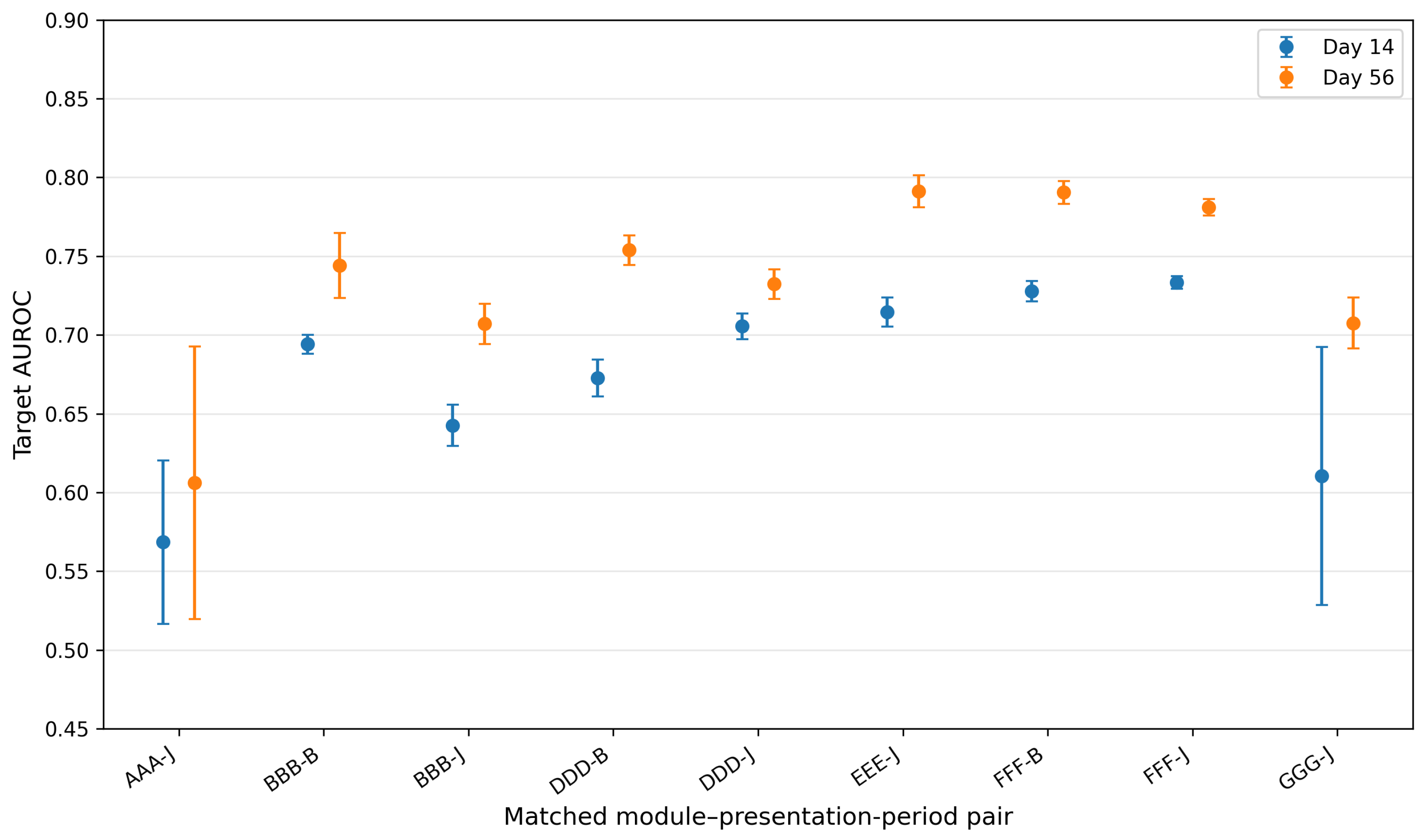
The OULAD release contains presentation labels 2013B, 2013J, 2014B, and 2014J; B presentations begin in February and J presentations begin in October [36]. Exact temporal matching used nine same-module, same-period pairs: AAA–J; BBB–B and BBB–J; DDD–B and DDD–J; EEE–J; FFF–B and FFF–J; and GGG–J. CCC lacked a 2013 match. Separate models were fitted for each pair at days 14 and 56. Results were aggregated both with equal pair weights and with target sample-size weights. A pooled sensitivity model added module and B/J presentation fixed effects. Module-mix change was quantified by total-variation and Jensen–Shannon distance.

The primary representation was score-free. It included baseline characteristics, previous attempts, studied credits, registration lead time, cumulative clicks, VLE record counts, active-day fraction, recency, activity rates, and resource-type shares. Assessment score was excluded because OULAD records date_submitted and score but not the time when a score became visible to a real decision-support system. A secondary day-56 sensitivity added assessment availability, submission, missed-assessment, and score summaries under the explicit assumption that recorded scores were available by the landmark.

3.7. South German Credit Evidence-Degradation Protocol

The adverse-credit target was the unfavorable credit-risk code. A total of 3 numeric variables (duration, amount, and age) and 17 categorical variables were perturbed in the original feature space before imputation and one-hot encoding. The fixed-count missingness condition set exactly three randomly selected features per test record to missing, independently of values and labels. Because the row-wise missing count was fixed, it is termed fixed-count MCAR-like rather than independent Bernoulli MCAR [48]. Random-feature-set deletion removed the same three features from every test case; 20 independently sampled three-feature sets were retained separately within each of 20 refits. Targeted deletion removed the three training-derived predictors with the highest mutual information. Mutual information used median-filled numeric values and integer-coded categorical values, with categorical variables declared discrete.

Measurement corruption independently affected 20% of values per feature. Numeric noise had a standard deviation 0.2 times the training standard deviation, was clipped to the observed training range, and duration and age were rounded. Categorical replacement sampled from the empirical training distribution after excluding the original category. A label-informed oracle/adversarial stress test replaced the three selected features in 30% of test cases with values from a training donor in the opposite class. It is reported separately and is not interpreted as a natural deployment error.

3.8. Heart Disease Source and Target Construction

The exact UCI files were processed.cleveland.data, processed.hungarian.data, processed.switzerland.data, and processed.va.data. Question marks were parsed as missing; no records were excluded. The multi-level disease variable was binarized as disease present when severity was greater than zero. The 13 predictors were age, sex, chest-pain type, resting blood pressure, cholesterol, fasting blood sugar, resting ECG, maximum heart rate, exercise-induced angina, oldpeak, slope, number of major vessels, and thal.

For each held-out site, the other three sites were pooled as the source domain. Source splits were stratified jointly by site and target. The primary logistic model used median/mode imputation without missingness indicators. The secondary model added imputation indicators, which may encode site-specific acquisition practice. Site sample sizes and positive/negative counts were Cleveland 303 (139/164), Hungary 294 (106/188), Switzerland 123 (115/8), and VA Long Beach 200 (149/51). The extreme Swiss imbalance makes negative-class estimates intrinsically imprecise.

3.9. Selective Prediction, Conformal Prediction, and Metrics

For confidence $c_i=max({\widehat{p}}_i,1-{\widehat{p}}_i)$, a source-calibrated threshold $\tau$ selected cases with $c_i\ge \tau$. Selection rate and selective risk were reported jointly. HCEP is the full-population high-confidence error burden and is not independent:

$$HCEP\left(\tau \right)=SelectionRate\left(\tau \right)\times SelectiveRisk\left(\tau \right).$$

(3)

For split-conformal classification, the nonconformity score was $s_i=1-{\widehat{p}}_{i,y_i}$. With n calibration scores and error level $\alpha$,

$$k=min\{n,\lceil (n+1)(1-\alpha )\rceil \},\widehat{q}=s_{\left(k\right)}.$$

(4)

A class was included when its score did not exceed $\widehat{q}$; ties were included, and no randomization was used. Marginal conformal prediction used one quantile. Label-conditional conformal prediction estimated separate class-0 and class-1 quantiles using the same finite-sample rank within each class. Outcomes were coverage, class-specific coverage, class-specific singleton accuracy, average set size, singleton rate, two-class ambiguity, and empty-set rate. OOD coverage is an empirical diagnostic, not a transported theoretical guarantee.

AP was computed with scikit-learn’s stepwise average-precision implementation rather than trapezoidal PR-AUC [42,49]. With prevalence $\pi$, PR skill was

$$PRSkill={\displaystyle \frac{AP-\pi }{1-\pi }},$$

(5)

so zero corresponds to the prevalence-only baseline and one to perfect ranking. ECE used 15 equal-width bins. Risk–selection curves sorted cases by descending confidence using a stable mergesort, retained all tied cases in input order, and integrated cumulative weighted risk over the attained selection-rate grid by the trapezoidal rule. Excess AURC subtracted the empirical correct-first ordering. Raw AURC is task-error-dependent and was interpreted only within task.

3.10. Variability, Paired Contrasts, and Reproducibility

Repeated refits were summarized by mean, standard deviation, median, and empirical range. Standard deviations describe split/fitting dispersion, not confidence intervals. Paired OOD-minus-ID changes used the same refit. ACS target-definition contrasts used 500 state-and-label-stratified weighted record bootstraps on one fixed target pipeline; this is not a replicate-weight survey analysis. OULAD used 500 two-stage resamples that sampled module–period pairs and then students within selected pairs on fixed primary predictions. South German Credit retained the complete random-feature-set distribution rather than averaging it away. Heart Disease class-specific coverage was accompanied in the machine-readable archive by exact Clopper–Pearson intervals for each refit.

Three post hoc diagnostic analyses were added without altering the primary analysis. First, the ACS unadjusted and CPI-constant targets were compared on the same 75,000 2024 records with two fixed primary prediction pipelines. For metric $M(y,p)$, four cells were evaluated: $M_{UU}$, $M_{UC}$, $M_{CU}$, and $M_{CC}$, where the first subscript is the unadjusted/CPI label definition and the second is the prediction pipeline. The symmetric target-label component was

$$D_Y=\frac{1}{2}[(M_{UU}-M_{CU})+(M_{UC}-M_{CC})],$$

(6)

and the prediction-pipeline component was

$$D_P=\frac{1}{2}[(M_{UU}-M_{UC})+(M_{CU}-M_{CC})],$$

(7)

so $D_Y+D_P=M_{UU}-M_{CC}$. This is an algebraic factor decomposition, not causal identification. As a second diagnostic, an intercept-only shift on the prediction logit aligned each pipeline’s weighted mean prediction to its corresponding target prevalence; 300 state-and-joint-label-stratified bootstraps quantified the residual difference after this prevalence/intercept alignment.

Second, marginal and label-conditional 90% conformal prediction were paired across 27 primary OOD/stress conditions: 3 ACS target definitions, 18 exact OULAD pair–horizon conditions, clean and targeted South German Credit, and 4 Heart Disease sites. This yielded 290 repeated paired comparisons. The main contrast was the change in worst-class coverage; average set size and singleton rate quantified the informativeness trade-off.

Third, a fixed LightGBM model was run under the same Platt-calibrated source-to-target protocol in all four domains. OOD-minus-ID changes in AUROC, ECE, and Brier score were then integrated with descriptive mixed-effects models. For the primary logistic model, random intercepts represented domain and condition-within-domain heterogeneity, with refit-level residual variation. A second model added model family as a fixed effect. With only four high-level domains, these models summarize observed variability and are not population-level meta-analyses.

The versioned reproducibility package contains executable preparation and analysis scripts, environment specifications, deterministic cohort and split manifests, feature dictionaries, harmonization tables, raw-input SHA-256 checksums, complete refit-level results, the added diagnostic-analysis outputs, and figure/table regeneration scripts. A result registry supplies manuscript values. Raw public datasets are not redistributed and must be placed in the documented input directory.

Only public, de-identified secondary data were used. No participants were recruited, and no clinical, educational, financial, or other deployment validity is claimed.

4. Results

4.1. Execution Completeness and Model Specification

Every pre-specified primary and secondary combination was retained in the machine-readable result matrix. The ACS matrix contains both model families and all three probability mappings for three target definitions, two domains, three conformal levels, two conformal methods, two weighting conventions, and five selection rates. OULAD contains 10 refits for each exact pair/horizon and each pooled sensitivity. Credit results retain 20 random feature sets within each of 20 refits. Heart Disease contains all four held-out sites, two missingness-indicator specifications, three probability mappings, two conformal methods, three conformal levels, and five selection rates. No result shown below was selected by target-domain performance.

4.2. ACS Target-Definition Sensitivity and Source-to-Target Transport

Table 4. Primary ACS results. Values are survey-weighted mean ± split/fitting SD across ten refits. AP is average precision.

Target Definition	Domain	Prevalence	AUROC	AP	Brier	Log Loss	ECE
Unadjusted reported	id test	0.356 ± 0.002	0.883 ± 0.002	0.797 ± 0.005	0.132 ± 0.001	0.408 ± 0.004	0.013 ± 0.003
Unadjusted reported	ood test	0.479 ± 0.000	0.873 ± 0.000	0.852 ± 0.000	0.158 ± 0.001	0.483 ± 0.002	0.099 ± 0.002
Survey-year adjusted	id test	0.384 ± 0.002	0.883 ± 0.003	0.815 ± 0.006	0.134 ± 0.002	0.417 ± 0.006	0.013 ± 0.003
Survey-year adjusted	ood test	0.510 ± 0.000	0.872 ± 0.000	0.865 ± 0.000	0.158 ± 0.001	0.485 ± 0.002	0.102 ± 0.002
CPI-constant 2018 USD	id test	0.384 ± 0.002	0.883 ± 0.003	0.815 ± 0.006	0.134 ± 0.002	0.417 ± 0.006	0.013 ± 0.003
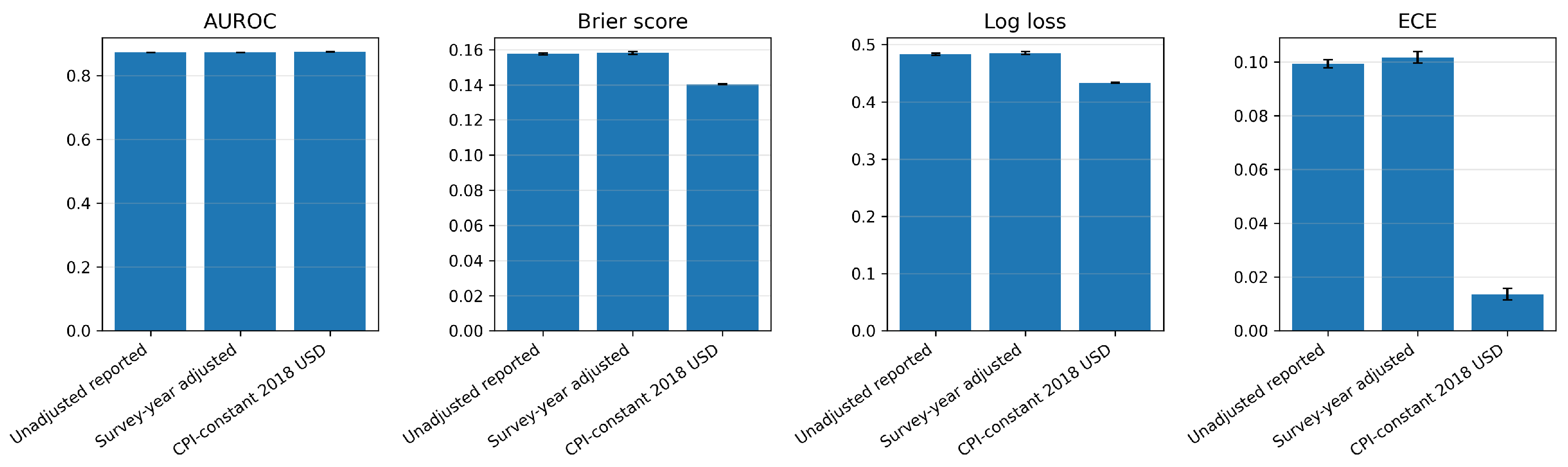
CPI-constant 2018 USD	ood test	0.396 ± 0.000	0.875 ± 0.000	0.807 ± 0.001	0.140 ± 0.000	0.434 ± 0.001	0.014 ± 0.002

uses the primary logistic–Platt pipeline. The source target is identical for the survey-year-adjusted and CPI-constant definitions in 2018, whereas the 2024 labels differ. Target AUROC changed little across definitions, but probability quality differed materially. The unadjusted construction had target ECE 0.099 and Brier score 0.158; the CPI-constant construction had ECE 0.014 and Brier score 0.140. The paired weighted bootstrap difference, unadjusted minus CPI-constant, was 0.082 [0.077, 0.087] for ECE, 0.017 [0.016, 0.019] for Brier score, and 0.047 [0.043, 0.051] for log loss. The AUROC difference was only −0.003 [−0.005, −0.000]. These results show target-definition sensitivity on identical records; they do not isolate one causal shift mechanism. The pattern is mechanistically plausible because AUROC depends on relative score ordering, whereas calibration and proper scores depend on the absolute relationship between scores and event frequencies. Relabeling a subset of otherwise identical records through a changed outcome threshold can therefore leave ordering nearly intact while changing the probability interpretation of those scores.

The same-record diagnostic sharpened that interpretation. The weighted prevalence was 0.47945 under the unadjusted target and 0.39581 under the CPI-constant target. The weighted label-change rate was 8.36%, entirely from unadjusted-positive to CPI-negative records; it therefore exactly matched the 8.36 percentage-point prevalence difference in this nested threshold construction.

Table 5. ACS same-record diagnostic decomposition, unadjusted minus CPI-constant target. Components are symmetric algebraic factor contributions on one fixed pair of primary pipelines. The final column is after intercept-only prevalence alignment and is not a causal estimand.

Metric	Total Difference	Target-Label Component	Prediction-Pipeline Component	Aligned Residual [95% Interval]
ECE	0.0826	0.0692	0.0133	−0.0039 [−0.0063, 0.0007]
Brier score	0.0169	0.0140	0.0030	0.0047 [0.0033, 0.0063]
Log loss	0.0467	0.0389	0.0078	0.0143 [0.0103, 0.0184]

separates the target-label and prediction-pipeline factors algebraically and then reports the residual after intercept-only prevalence alignment. For ECE, the target-label factor accounted for 0.0692 of the total 0.0826 contrast, while the prediction-pipeline factor accounted for 0.0133. Prevalence/intercept alignment reduced the ECE contrast to $-0.0039$ with a diagnostic 95% bootstrap interval spanning zero. Brier score and log loss retained smaller positive residual differences. Thus, the large ECE contrast is predominantly consistent with changed prevalence/calibration intercept, while proper-score differences show that prevalence alignment does not erase all target-definition sensitivity. Neither decomposition identifies a causal concept-shift effect. The broader implication is that target semantics and probability semantics are coupled: changing what the target operationally means can substantially change probability reliability without materially changing discrimination.

Figure 2 summarizes the corresponding target-domain results for the primary logistic–Platt pipeline.

For the CPI-constant target, transferring the source threshold intended to select 80% of cases yielded target selection rate 0.791 and selective risk 0.144, compared with source values 0.800 and 0.135. Marginal 90% empirical target coverage was 0.896 with average set size 1.237; label-conditional coverage was 0.895, with class-0/class-1 coverage 0.898/0.891. Under the unadjusted target, marginal class-1 coverage fell to 0.784.

Five independently sampled computational cohorts reproduced the substantive pattern. For the CPI-constant target, target AUROC was 0.875 ± 0.002 and ECE was 0.012 ± 0.003; for the unadjusted target, target ECE was 0.103 ± 0.006. The secondary LightGBM and alternative mapping grid did not alter the conclusion that ranking was comparatively stable while the nominal target constructions produced poorer probability calibration. Raw, Platt, and isotonic target ECE for LightGBM under the CPI-constant target were 0.012, 0.015, and 0.016, respectively.

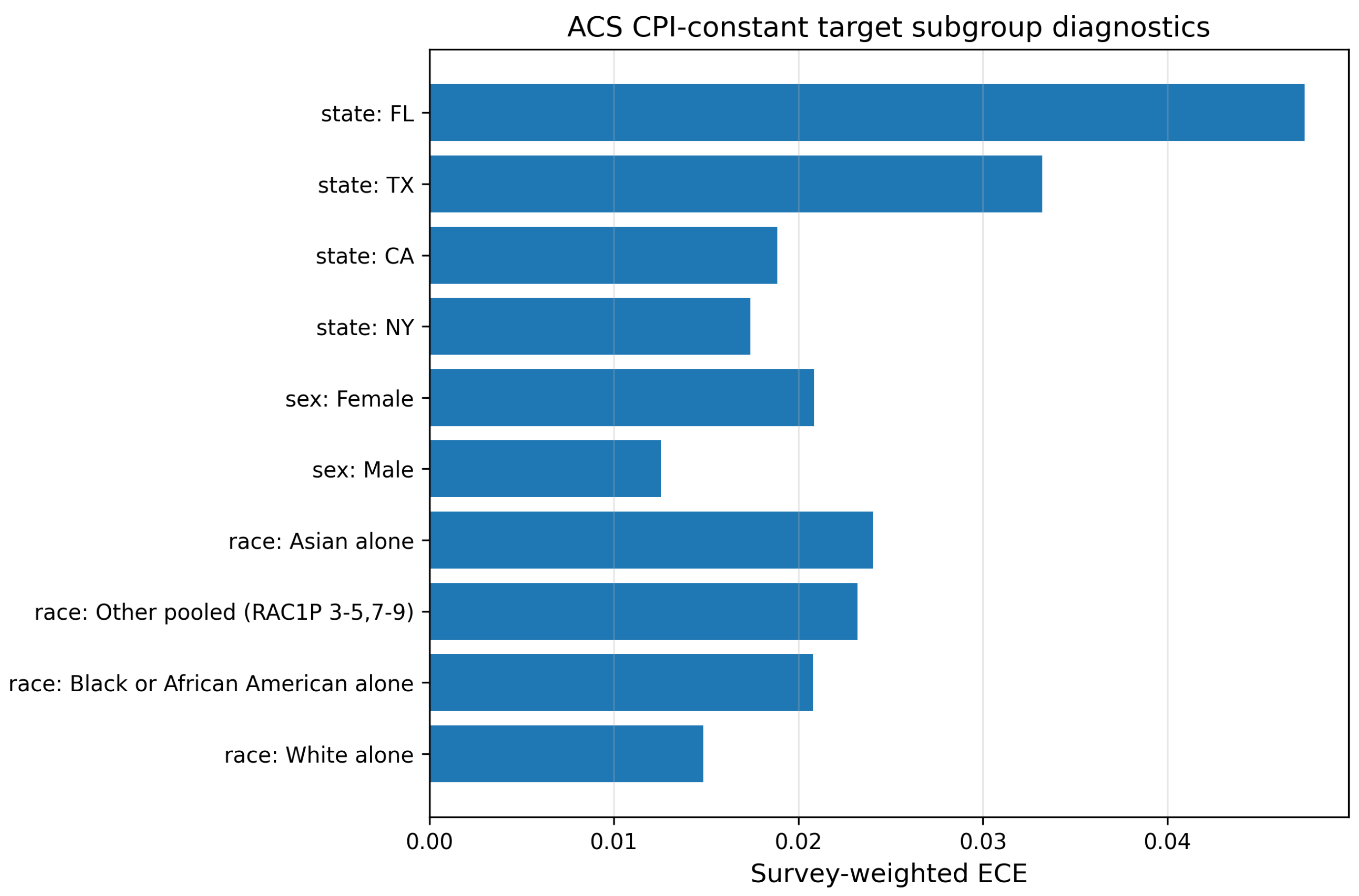
The fixed-refit subgroup diagnostic found survey-weighted ECE values from 0.013 to 0.047 across states and sexes and from 0.015 to 0.024 across the four reported race groups. These are descriptive subgroup diagnostics, not a fairness analysis. Figure 3 shows the complete fixed-refit values.

4.3. OULAD Exact Temporal Matching, Estimand Sensitivity, and Conformal Asymmetry

Table 6. OULAD exact-pair aggregate results. Values are mean ± split/fitting SD across ten refits. Marginal and LC columns report class-1 empirical coverage at nominal 90%.

Horizon/Aggregation	Domain	AUROC	AP	Brier	ECE	Marg. Cov.	Marg. Class 1	LC Class 1
Day 14, equal pair	id test	0.708 ± 0.019	0.662 ± 0.023	0.204 ± 0.004	0.081 ± 0.009	0.901 ± 0.009	0.823 ± 0.020	0.889 ± 0.019
Day 14, equal pair	ood test	0.674 ± 0.007	0.585 ± 0.006	0.213 ± 0.002	0.054 ± 0.009	0.889 ± 0.008	0.778 ± 0.023	0.845 ± 0.013
Day 14, size weighted	ood test	0.688 ± 0.005	0.608 ± 0.005	0.215 ± 0.002	0.056 ± 0.010	0.881 ± 0.009	0.770 ± 0.021	0.825 ± 0.021
Day 56, equal pair	id test	0.744 ± 0.018	0.695 ± 0.017	0.186 ± 0.003	0.084 ± 0.010	0.904 ± 0.012	0.801 ± 0.028	0.905 ± 0.021
Day 56, equal pair	ood test	0.735 ± 0.009	0.661 ± 0.008	0.191 ± 0.002	0.066 ± 0.007	0.905 ± 0.011	0.795 ± 0.029	0.885 ± 0.024
Day 56, size weighted	ood test	0.747 ± 0.003	0.683 ± 0.004	0.193 ± 0.003	0.070 ± 0.010	0.895 ± 0.012	0.777 ± 0.034	0.863 ± 0.034

separates equal-pair and sample-size-weighted summaries. Equal-pair target AUROC was 0.674 at day 14 and 0.735 at day 56. The corresponding size-weighted values were 0.688 and 0.747. OOD-minus-ID AUROC changes were −0.034 and −0.009 for equal-pair summaries. The target-sample two-stage bootstrap intervals were [0.636, 0.706] at day 14 and [0.706, 0.772] at day 56 for equal-pair AUROC. These intervals include pair and student resampling conditional on the fixed primary predictions.

Pair-level sample sizes, prevalences, and target results are shown in

Table 7. OULAD exact module–period pairs. $n_S/n_T$ and ${\pi }_S/{\pi }_T$ denote source/target sample size and prevalence. Coverage columns refer to target class 1 at day 14.

Pair	${\mathit{n}}_{\mathit{S}}/{\mathit{n}}_{\mathit{T}}$ D14	${\mathit{\pi }}_{\mathit{S}}/{\mathit{\pi }}_{\mathit{T}}$ D14	AUROC D14	Marg. C1	LC C1	${\mathit{n}}_{\mathit{S}}/{\mathit{n}}_{\mathit{T}}$ D56	${\mathit{\pi }}_{\mathit{S}}/{\mathit{\pi }}_{\mathit{T}}$ D56	AUROC D56
AAA-J	370/318	0.249/0.258	0.568 ± 0.052	0.701	0.890	365/315	0.238/0.248	0.606 ± 0.087
BBB-B	1606/1257	0.501/0.427	0.694 ± 0.006	0.860	0.863	1470/1216	0.454/0.406	0.744 ± 0.021
BBB-J	1851/1760	0.422/0.359	0.643 ± 0.013	0.443	0.544	1785/1723	0.399/0.338	0.707 ± 0.013
DDD-B	1197/1008	0.575/0.534	0.673 ± 0.012	0.908	0.843	1085/933	0.530/0.496	0.754 ± 0.009
DDD-J	1675/1381	0.507/0.445	0.705 ± 0.008	0.894	0.896	1574/1331	0.474/0.424	0.732 ± 0.009
EEE-J	933/1003	0.348/0.324	0.715 ± 0.009	0.737	0.878	906/974	0.328/0.304	0.791 ± 0.010
FFF-B	1520/1264	0.486/0.495	0.728 ± 0.006	0.874	0.896	1407/1214	0.444/0.473	0.790 ± 0.007
FFF-J	1998/1800	0.452/0.393	0.733 ± 0.004	0.810	0.884	1915/1714	0.428/0.361	0.781 ± 0.005
GGG-J	926/717	0.361/0.382	0.610 ± 0.082	0.777	0.908	919/696	0.356/0.364	0.708 ± 0.016

. Considerable heterogeneity remained after exact module–period matching. Exact matching controls observed module and presentation-period labels, but it cannot hold constant unrecorded year-specific changes in curriculum delivery, assessment design, learner support, or student composition within those cells. Fixed effects likewise adjust recorded strata rather than unmeasured time-varying mechanisms. Residual pair heterogeneity therefore cannot be interpreted as a pure temporal effect. Equal weighting answers the average-pair question, while sample-size weighting answers the average-observation question; neither is universally preferable.

Figure 4 shows target AUROC for each exact OULAD module–presentation-period pair.

The landmark and all-registered estimands yielded materially different results. In pooled fixed-effect models, day-14 target AUROC was 0.728 for the score-free landmark cohort but 0.796 when all students registered by the horizon, including early withdrawals, were retained. At day 56, the corresponding values were 0.776 and 0.856. These are different prediction targets rather than evidence that one model specification is intrinsically superior. The difference is inseparable from the risk-set estimand because landmark analysis conditions on still being registered and not yet withdrawn at day t, thereby excluding earlier withdrawals, whereas the all-registered analysis retains those learners and counts their later status in the outcome. Eligibility, prevalence, and case mix therefore change by construction when the estimand changes. Adding assessment/score summaries to the day-56 landmark model increased target AUROC from 0.776 to 0.819, but the availability time of scores is not verifiable in OULAD; this result remains secondary.

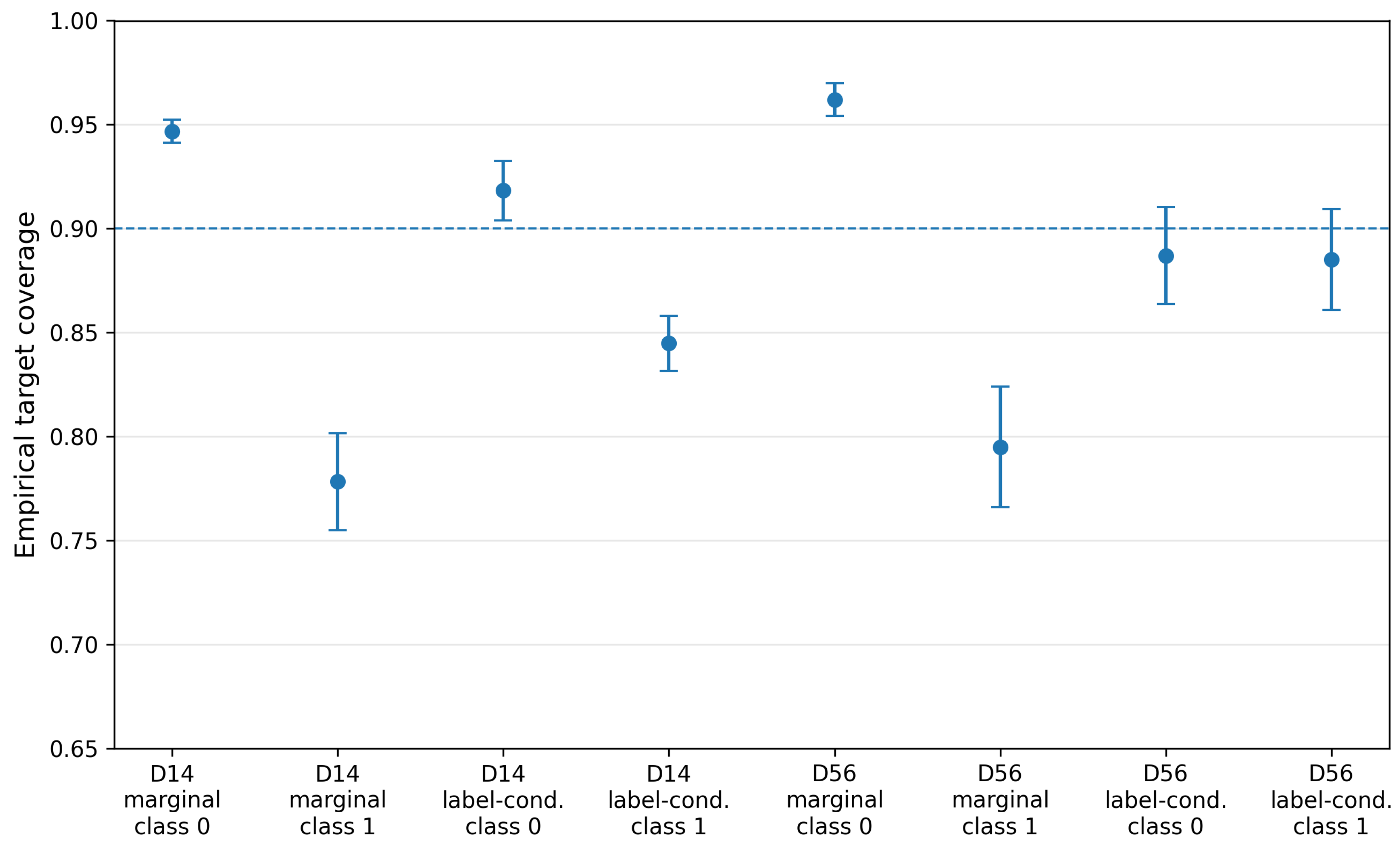
Marginal conformal coverage concealed asymmetric outcome coverage. At day 14, equal-pair target marginal coverage was 0.889, but class-1 coverage was 0.778. Label-conditional calibration raised class-1 coverage to 0.845 at average set size 1.596. At day 56, marginal and label-conditional class-1 coverage were 0.795 and 0.885. The gain was accompanied by lower singleton informativeness.

Figure 5 shows the class-specific target coverage under marginal and label-conditional conformal prediction.

4.4. Equal-Budget Credit Degradation

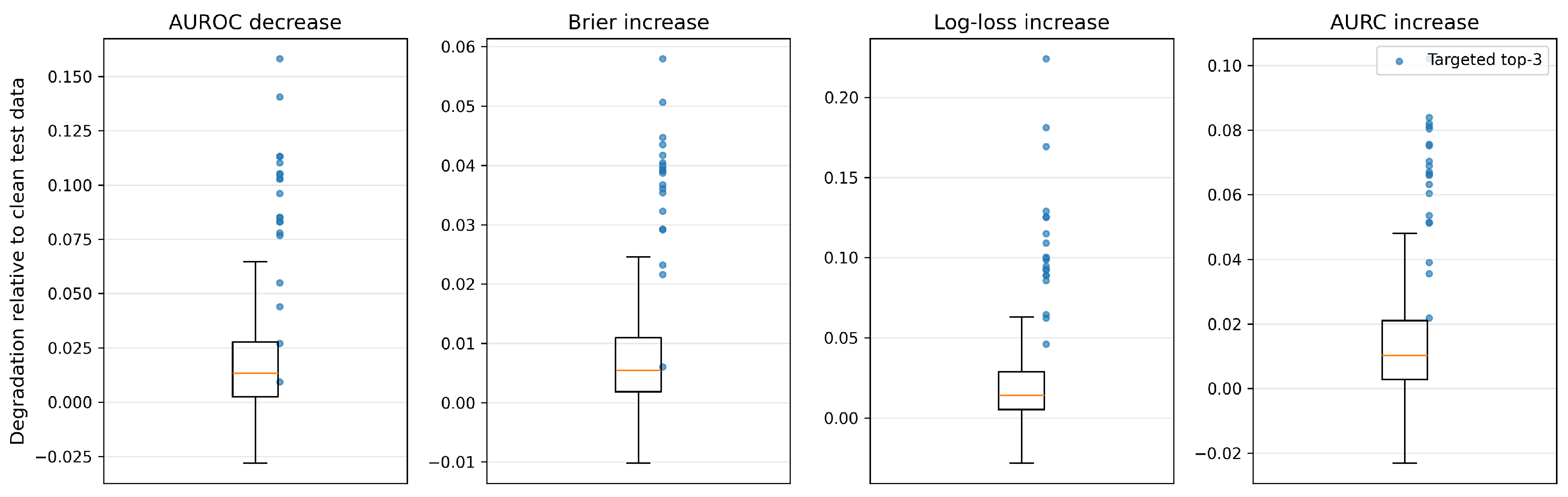
The primary clean credit AUROC was 0.784. Removing three random features produced mean AUROC 0.765, whereas removing the three highest-mutual-information features produced 0.695. Across refits, the targeted AUROC degradation was on average at the 94th percentile of the 20 random-set degradation distribution. Checking-account status appeared in the top three in all 20 refits, credit history in 14, and duration in 13; the selected set was not completely stable. The equal missing-feature count therefore does not imply equal informational loss: targeted deletion preferentially removes variables with stronger source-sample dependence on the outcome, while random deletion often removes more redundant or weakly informative variables. Because mutual information is associative rather than causal, this explains the stress-test construction without identifying those variables as causal determinants.

Table 8. South German Credit primary stress results. Values are mean ± dispersion across refits and, for random deletion, retained feature-set draws. LC: label conditional.

Condition	AUROC	AP	Brier	ECE	Marg. Cov.	Marg. C1	LC C1
Clean	0.784 ± 0.048	0.626 ± 0.071	0.166 ± 0.016	0.089 ± 0.021	0.900 ± 0.039	0.717 ± 0.111	0.892 ± 0.086
Fixed-count MCAR-like	0.767 ± 0.050	0.601 ± 0.071	0.171 ± 0.016	0.082 ± 0.021	0.887 ± 0.040	0.654 ± 0.124	0.871 ± 0.105
Random three-feature deletion	0.765 ± 0.049	0.598 ± 0.070	0.175 ± 0.018	0.102 ± 0.029	0.886 ± 0.053	0.653 ± 0.179	0.866 ± 0.117
Targeted top-three deletion	0.695 ± 0.055	0.531 ± 0.075	0.202 ± 0.014	0.126 ± 0.032	0.800 ± 0.049	0.332 ± 0.164	0.710 ± 0.180
Measurement/category corruption	0.707 ± 0.058	0.528 ± 0.067	0.191 ± 0.019	0.105 ± 0.033	0.859 ± 0.044	0.592 ± 0.120	0.822 ± 0.104

summarizes the primary South German Credit stress-test results.

Targeted deletion reduced marginal 90% coverage to 0.800, compared with 0.886 under random three-feature deletion. The main shortfall occurred in adverse-credit class 1, where marginal coverage was 0.332. Label-conditional conformal prediction raised that value to 0.710 but produced larger sets. The label-informed oracle/adversarial stress yielded AUROC 0.693 and is not compared as an equally realistic deployment process.

Figure 6 contrasts the degradation distributions for random and targeted three-feature deletion.

4.5. Heart Disease Institutional Transfer

Table 9. Heart Disease primary leave-one-site-out results. Positive/negative target counts are shown after the site name. Values are mean ± split/fitting SD. Marg.: marginal conformal; LC: label conditional.

Target Site (+/−)	ID AUROC	OOD AUROC	OOD ECE	Sel. Rate	Sel. Risk	Marg. Cov.	Marg. C0	Marg. C1	LC C0	LC C1
Cleveland (139/164)	0.894 ± 0.025	0.751 ± 0.141	0.176 ± 0.111	0.762 ± 0.108	0.275 ± 0.135	0.814 ± 0.126	0.834 ± 0.223	0.789 ± 0.131	0.903 ± 0.188	0.741 ± 0.169
Hungary (106/188)	0.873 ± 0.027	0.874 ± 0.009	0.111 ± 0.036	0.732 ± 0.089	0.128 ± 0.023	0.916 ± 0.023	0.929 ± 0.021	0.892 ± 0.050	0.990 ± 0.011	0.815 ± 0.067
Switzerland (115/8)	0.892 ± 0.034	0.742 ± 0.013	0.334 ± 0.046	0.678 ± 0.046	0.268 ± 0.068	0.829 ± 0.068	0.750 ± 0.059	0.835 ± 0.071	0.775 ± 0.053	0.823 ± 0.086
VA Long Beach (149/51)	0.908 ± 0.026	0.704 ± 0.014	0.139 ± 0.036	0.734 ± 0.096	0.216 ± 0.021	0.856 ± 0.053	0.686 ± 0.119	0.915 ± 0.036	0.733 ± 0.066	0.907 ± 0.045

reports the primary no-indicator logistic–Platt model. The other three sites formed the source domain in each row. Target AUROC ranged from 0.704 at VA Long Beach to 0.874 in Hungary. The Swiss ECE was 0.334, but the site contained only eight negative records. Source-calibrated 0.80 selection thresholds achieved target selection rates from 0.678 to 0.762, with target selective risk from 0.128 to 0.275. This institutional heterogeneity can arise from several coupled sources, including different prevalence, predictor distributions, measurement and missingness patterns, and small target samples. The leave-one-site-out design reveals that source operating properties need not transport, but it cannot attribute each site effect to one of these mechanisms.

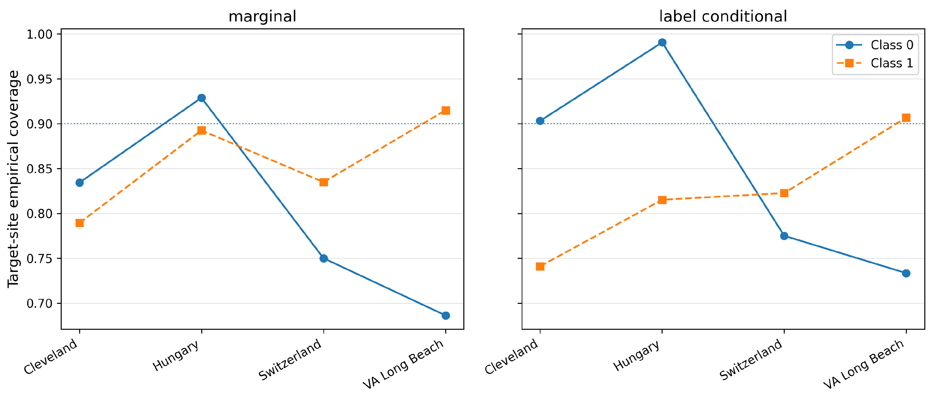
Marginal target coverage was lowest for Cleveland at 0.814. Class-specific results were more heterogeneous: marginal class-0 coverage was 0.686 at VA Long Beach and 0.750 in Switzerland. Label-conditional calibration increased some undercovered classes but did not restore nominal target coverage consistently. This is expected because class conditioning addresses source-domain class imbalance, not arbitrary institutional shift.

Figure 7 shows target-site class-specific empirical coverage for the two conformal calibration strategies.

Adding missingness indicators changed target AUROC by +0.053 for Cleveland, +0.011 for Hungary, −0.033 for Switzerland, and −0.019 for VA Long Beach on average. ECE changed in different directions. Missingness patterns can therefore carry site identity and predictive signal without being reliably transportable.

4.6. Label-Conditional Conformal Calibration Is a Trade-Off, Not a Universal Repair

Across the 27 primary 90% OOD/stress conditions, label-conditional calibration increased mean worst-class coverage in 18 conditions and decreased it in 9. At the repeated-comparison level, worst-class coverage improved in 205 of 290 comparisons, worsened in 70, and was unchanged in 15. Prediction sets became larger in 221 of 290 comparisons (76.2%). The trade-off was not confined to small datasets: the worst mean change occurred for Heart Disease Hungary ($-0.0679$), while OULAD BBB-B at day 56 changed by $-0.0569$. Conversely, targeted top-three credit deletion improved worst-class coverage by 0.3778 but increased average set size by 0.3417. Label conditioning therefore often protects a weak class, but it is not a distribution-shift correction and can worsen the minimum class coverage or reduce informativeness. The reason is structural: each class receives a source-calibrated quantile estimated from a smaller class-specific calibration subset, and arbitrary target shift may alter the class-specific nonconformity distributions differently. Separate source quantiles can therefore correct source imbalance while still being too liberal or too conservative for a shifted target class, with finite-sample quantile coarseness amplifying the effect in small classes.

4.7. Model-Family Sensitivity Across All Four Domains

LightGBM changed absolute discrimination and probability metrics, sometimes substantially, but did not remove the need for the multi-output audit.

Table 10. Representative post hoc model-family sensitivity. Values are mean target/stress metrics across refits. Worst cov. is worst-class marginal 90% conformal coverage.

Condition	LR AUROC	LGBM AUROC	LR ECE	LGBM ECE	LR Worst Cov.	LGBM Worst Cov.
ACS unadjusted target	0.873	0.876	0.099	0.101	0.784	0.780
ACS CPI-constant target	0.875	0.877	0.014	0.015	0.866	0.862
OULAD pooled day 56	0.776	0.759	0.027	0.042	0.806	0.828
Credit targeted top-three	0.695	0.660	0.126	0.108	0.332	0.360
Heart Cleveland	0.751	0.839	0.176	0.102	0.718	0.871
Heart VA Long Beach	0.704	0.677	0.139	0.202	0.686	0.706

gives representative OOD/stress conditions using the same Platt-calibrated transport protocol. Cleveland Heart Disease improved strongly with LightGBM, whereas OULAD day 56, targeted credit deletion, and VA Long Beach did not. In ACS, both model families retained the large calibration contrast between the unadjusted and CPI-constant targets despite similar AUROC. The model-family analysis therefore supports the use of logistic regression as an audit probe while showing that absolute results should not be treated as architecture-invariant.

4.8. Statistical Integration of Cross-Domain Variability

The descriptive mixed-effects integration separates domain, condition, and refit variation rather than pooling all observations as independent. For the primary logistic model, the estimated mean OOD-minus-ID shift was $-0.059$ for AUROC, +0.054 for ECE, and +0.032 for Brier score. For AUROC, 29.6% of the estimated variance was at the domain level, 43.0% at the condition-within-domain level, and 27.4% at the refit level. For ECE, the corresponding fractions were approximately 0.0%, 72.1%, and 27.9%; for Brier score, they were 29.3%, 29.9%, and 40.8%. In the model-family extension, the LightGBM-minus-logistic change in the OOD shift was $-0.001$ for AUROC, $-0.007$ for ECE, and $-0.002$ for Brier score. The concentration of ECE variability at the condition level is consistent with calibration being especially sensitive to the particular prevalence, target-definition, evidence, or site change imposed within a domain, whereas AUROC variability was distributed more broadly across domain and condition levels. This interpretation remains descriptive rather than mechanistic proof. These small average model-family shift differences coexist with large condition-specific absolute differences and should be read descriptively because only four domain families were observed.

4.9. What Is Cross-Domain Evidence and What Remains Case-Specific

The four datasets are separate empirical test beds, not interchangeable replications of one data-generating process. The bounded cross-domain result is that reliability conclusions changed when evaluation moved beyond ranking to probability quality, transported operating rules, or class-specific uncertainty; the size and mechanism of those changes were domain dependent. The target-definition/prevalence result is specific to ACS, the estimand and module-composition result to OULAD, the informational-relevance result to controlled credit degradation, and the site/missingness heterogeneity result to Heart Disease. CRIT-AID therefore supports a common audit logic across domains without claiming that one numerical effect has been universally proven.

5. Discussion

5.1. Distinguishing the CRIT-AID Framework from the CRIT-AID Protocol

The individual ingredients of this study are established statistical procedures. CRIT-AID names the overall empirical audit framework, whereas the CRIT-AID protocol names the mandatory execution contract that governs how those ingredients are combined. A conforming protocol execution must declare the target estimand and evidence-availability time, preserve disjoint fitting/calibration/test roles, compare source and target outputs under the same metric definitions, transport source-derived selection and conformal rules without target tuning, expose target-definition alternatives when substantively plausible, and report class-specific validity together with prediction-set informativeness. The broader CRIT-AID framework additionally includes the stress-test catalogue, interpretation logic, common result schema, and reproducibility record. This distinction makes clear why CRIT-AID is closer to a reproducible audit specification than to a new learning algorithm. The comparison with NIST AI RMF, Model Cards, the ML Test Score, and distribution-shift benchmarks also clarifies its boundary: CRIT-AID supplies a narrow empirical reliability layer and does not replace governance, documentation, or socio-technical risk management [1,2,3,31,32].

5.2. Stable Discrimination Is Insufficient Evidence of Reliable Decision Support

The main conceptual implication is that stable discrimination cannot certify the reliability of quantities downstream from ranking. A stable AUROC is not evidence that deployed probabilities, abstention thresholds, or uncertainty sets retain their source-domain interpretation. Calibration, proper scores, selection thresholds, and set-valued uncertainty depend on more than pairwise ordering. The ACS decomposition makes this distinction particularly concrete: changing a target threshold can preserve much of the ordering while changing prevalence and the calibration intercept enough to alter probability reliability. The appropriate response is not to discard AUROC but to prevent it from acting as a proxy for properties it does not measure.

5.3. Conditional Validity and Informativeness Must Be Evaluated Together

Label-conditional conformal calibration is useful when marginal coverage hides outcome asymmetry, but it should not be presented as a universal correction for deployment shift. Class-specific calibration samples are smaller, attainable quantiles are coarser, and target shift can affect the two classes differently. The 27-condition comparison demonstrates both directions of change: label-conditional calibration redistributed reliability rather than monotonically improving it. Improving conditional coverage can therefore trade reliability in one dimension for informativeness in another. A more defensible reporting rule is to show worst-class coverage, average set size, singleton rate, and relevant class sample sizes together. A method that raises coverage only by returning less informative sets has made a real trade-off rather than an unqualified reliability improvement.

5.4. Why Logistic Regression Remains Primary and What Model Complexity Changes

Logistic regression was retained as the primary audit probe because this study targets reliability transport rather than leaderboard prediction. The cross-domain LightGBM extension shows why model-family sensitivity still matters: a stronger nonlinear model can materially improve one site while worsening another, yet calibration and uncertainty failures can remain. This is compatible with evidence that tree ensembles are strong tabular baselines [24] and that calibration, selective prediction, and shift detection remain separate reliability objectives even for contemporary foundation-model fine-tuning [25]. The result does not establish invariance to deep tabular networks, foundation models, ensembles, or continually adapted systems; those remain external-validity questions.

5.5. A Lightweight Bridge from Technical Reliability to Human Factors

A technical audit should feed, rather than substitute for, human-factors evaluation. Five lightweight steps follow from the present framework. (1) Map every audited model output to the actual human action it can trigger, including escalation and abstention. (2) Present probability or set-valued uncertainty in the same interface format used in practice, because format can change reliance. (3) Oversample cases identified by the technical audit as high-confidence errors, class-specific undercoverage, or severe shift failures in user studies. (4) Measure behavior, such as override, verification, escalation, and error correction, rather than self-reported trust alone. (5) Monitor technical reliability and human reliance jointly after deployment, with predefined review triggers when either changes. These steps are consistent with the distinction between technical model validity and appropriate reliance emphasized in human–AI decision research and risk-management guidance [1,21].

5.6. Reproducibility as Part of Audit Validity

Multi-domain reliability claims are vulnerable to silent specification drift because results can change with the target definition, representation, calibration mapping, split, or aggregation rule. The release therefore treats machine-readable result matrices, deterministic manifests, explicit post hoc labels, citation metadata, and one bibliographic title as part of the audit record rather than supplementary decoration. This does not make the findings universally generalizable, but it makes the exact evidence and its boundaries independently inspectable.

6. Limitations

External validity is bounded by four public binary tabular test beds. The data are not uniformly small: ACS preparation contained 1,097,452 eligible records and OULAD preparation contained 130,372 registration–horizon candidates, but the South German Credit dataset has 1000 cases and the multi-site Heart Disease dataset has 920 historical records. Small-sample clinical prediction models can be unstable, and healthcare robustness comprises multiple distinct concepts beyond discrimination [50,51]. This study does not cover contemporary large-scale production logs, continuous monitoring streams, multi-class or regression decisions, multi-modal systems, large language models, AI agents, or systems that update online. The results should therefore motivate audit dimensions, not be extrapolated as effect sizes for modern operational AI.

Model-family sensitivity is limited to a fixed LightGBM specification in addition to logistic regression. No deep tabular architecture, foundation model, extensive ensemble, or target-tuned hyperparameter search was evaluated. The analysis shows that the central audit problem is not unique to one low-capacity classifier, but it cannot establish architecture-independent effect sizes.

The ACS same-record decomposition is diagnostic rather than causal. The CPI-constant threshold is nested within the unadjusted threshold on the analyzed 2024 records, so the observed 8.36% weighted label-change rate equals the prevalence difference and all changes occur in one direction. The two-factor metric decomposition and intercept-only prevalence alignment separate calculable components but do not identify covariate, label, prevalence, and concept shift as independent causal mechanisms. The survey-weighted bootstrap is not a replicate-weight analysis of the complete ACS complex survey design.

OULAD uses selected 2013B/J and 2014B/J module presentations rather than continuous longitudinal follow-up. Exact matching, fixed effects, and pair resampling reduce but do not eliminate curriculum, assessment, and composition confounding because these procedures condition only on recorded module/presentation structure and observed samples; they cannot hold constant unmeasured year-specific changes in teaching, assessment policy, learner support, or entrant composition. Fail and Withdrawn combine heterogeneous mechanisms. Later landmark estimates condition on remaining registered, so early withdrawal changes the eligible risk set by design, and score-inclusive results depend on an unverifiable score-availability assumption.

The cross-domain mixed-effects analysis includes only four high-level domain families and ten model-family sensitivity conditions. Variance components are therefore descriptive decompositions of this benchmark rather than estimates from a representative population of AI applications. Refit observations also share source datasets and should not be interpreted as independent studies.

Ordinary marginal and label-conditional split conformal prediction were used. Target coverage is empirical rather than theoretically guaranteed under arbitrary shift. Label conditioning can improve or worsen worst-class coverage and may increase set size. Small Heart Disease calibration classes produce coarse ranks and unstable class-specific estimates, especially for the eight Swiss negative records.

ECE uses 15 equal-width bins and is not a proper score [27]; for this reason, Brier score and log loss accompany it. Average precision is prevalence-sensitive, and AURC depends on underlying task error and implementation details. The fixed-count credit condition is MCAR-like rather than independent Bernoulli MCAR, while the label-informed oracle/adversarial condition is deliberately unrealistic and is reported only as a stress bound.

Finally, no human participants were studied. Technical reliability, appropriate reliance, trust, automation bias, verification behavior, and downstream harm are distinct constructs. The proposed human-factors bridge is a design recommendation for subsequent evaluation, not an empirically validated human-use result from this study.

7. Future Research Directions

The findings and limitations define a concrete extension program. First, the same audit contract should be prospectively replicated on contemporary large-scale operational data, including multi-class and regression decisions, streaming systems, multi-modal models, large language models, and tool-using agents. Such studies should preserve the central design principle of separating model fitting, calibration, operating-rule selection, and target evaluation rather than importing target-test tuning.

Second, architecture sensitivity should be expanded beyond one tree ensemble to deep tabular models, ensembles, foundation models, and systems that update online. The relevant question is not only whether a more complex model improves average prediction but whether it changes the transportability of calibration maps, abstention thresholds, and uncertainty sets; contemporary foundation-model work already demonstrates that calibration and shift-sensitive uncertainty require dedicated treatment [25]. Third, target-definition sensitivity should be studied in settings where policy, diagnostic, or eligibility definitions change prospectively, allowing richer decomposition of prevalence, relabeling, covariate, and mechanism changes than the diagnostic ACS contrast permits.

Fourth, conformal research should compare marginal and label-conditional procedures with shift-aware, generalized-shift, richer conditional-coverage, or risk-controlling alternatives while reporting coverage and informativeness jointly [20,29,30]. The present results make the coverage–set-size frontier, small-class quantile instability, and class-specific target shift natural primary outcomes rather than secondary diagnostics. Fifth, technical audit outputs should be carried into controlled and field-based human-factors studies that measure verification, override, escalation, and error correction on the specific high-confidence-error and undercoverage cases discovered by the audit. Finally, future benchmark expansion should increase the number of independent domains and pre-register application-specific tolerances so that variance components, failure frequencies, and pass/fail rules can be estimated with stronger external validity.

8. Conclusions

Stable discrimination is not sufficient evidence of reliable AI decision support. Across four heterogeneous tabular test beds, discrimination, probability calibration, selective operating points, and conformal uncertainty did not behave as interchangeable properties under target shift or evidence degradation. Probability calibration, selective operating points, and uncertainty sets can change materially even when ranking changes little. The strongest target-definition contrast was largely associated with prevalence/calibration-intercept change but retained smaller proper-score residuals after alignment, showing that target semantics can change probability reliability without materially changing discrimination. Label-conditional conformal calibration improved worst-class coverage in most primary conditions but worsened it in others and frequently enlarged prediction sets, demonstrating a coverage–informativeness trade-off rather than a universal repair. A fixed cross-domain LightGBM analysis changed absolute performance without eliminating the need to audit these separate reliability outputs.

The practical implication is a reporting principle rather than a new predictive algorithm: define the target before fitting; separate model, probability-calibration, selection/conformal-calibration, and test data; transfer operating rules without target tuning when transport is being audited; evaluate proper scores and calibration alongside discrimination; report achieved selection rate with selective risk; pair marginal conformal coverage with class-specific coverage and set informativeness; stress the informational relevance of missing evidence; and state clearly which conclusions are cross-domain patterns and which are case-specific.

CRIT-AID is intended as an executable technical reliability layer that can sit beneath broader governance and human-factors evaluation. Relative to adjacent frameworks, its comparative advantages are specific to this technical-audit task rather than universal superiority. Robustness is made directly testable by transporting source-derived probability mappings, selection thresholds, and conformal rules unchanged across natural or controlled shifts and by varying target semantics and evidence relevance. Reproducibility is strengthened by deterministic cohort and split manifests, versioned configurations, machine-readable result matrices, and regeneration scripts. Auditability is strengthened by explicit separation of fitting, calibration, selection/conformal calibration, and test roles, which makes leakage, target tuning, and metric-specific trade-offs inspectable. NIST AI RMF, Model Cards, and production-readiness frameworks retain broader governance, documentation, and socio-technical roles that CRIT-AID does not replace.

Its most general claim is deliberately narrow and testable: stable discrimination does not imply reliable probabilities, operating rules, or uncertainty under distribution shift. When AI decision support relies on probabilities, abstention rules, or uncertainty sets, stable discrimination alone cannot establish that those downstream quantities retain their source-domain interpretation after deployment conditions or target definitions change.