Article

Adaptive Multi-Scale Feature Fusion with Hybrid Representation Learning to Classify and Retrieve Histopathological Images

Computer Science Department, Faculty of Mathematics, Statistics and Computer Science, University of Tabriz, Tabriz 51666-16471, Iran
*
Author to whom correspondence should be addressed.
Computers 2026, 15(8), 473; https://doi.org/10.3390/computers15080473
Submission received: 26 May 2026 / Revised: 18 June 2026 / Accepted: 12 July 2026 / Published: 24 July 2026
(This article belongs to the Section AI-Driven Innovations)

Abstract

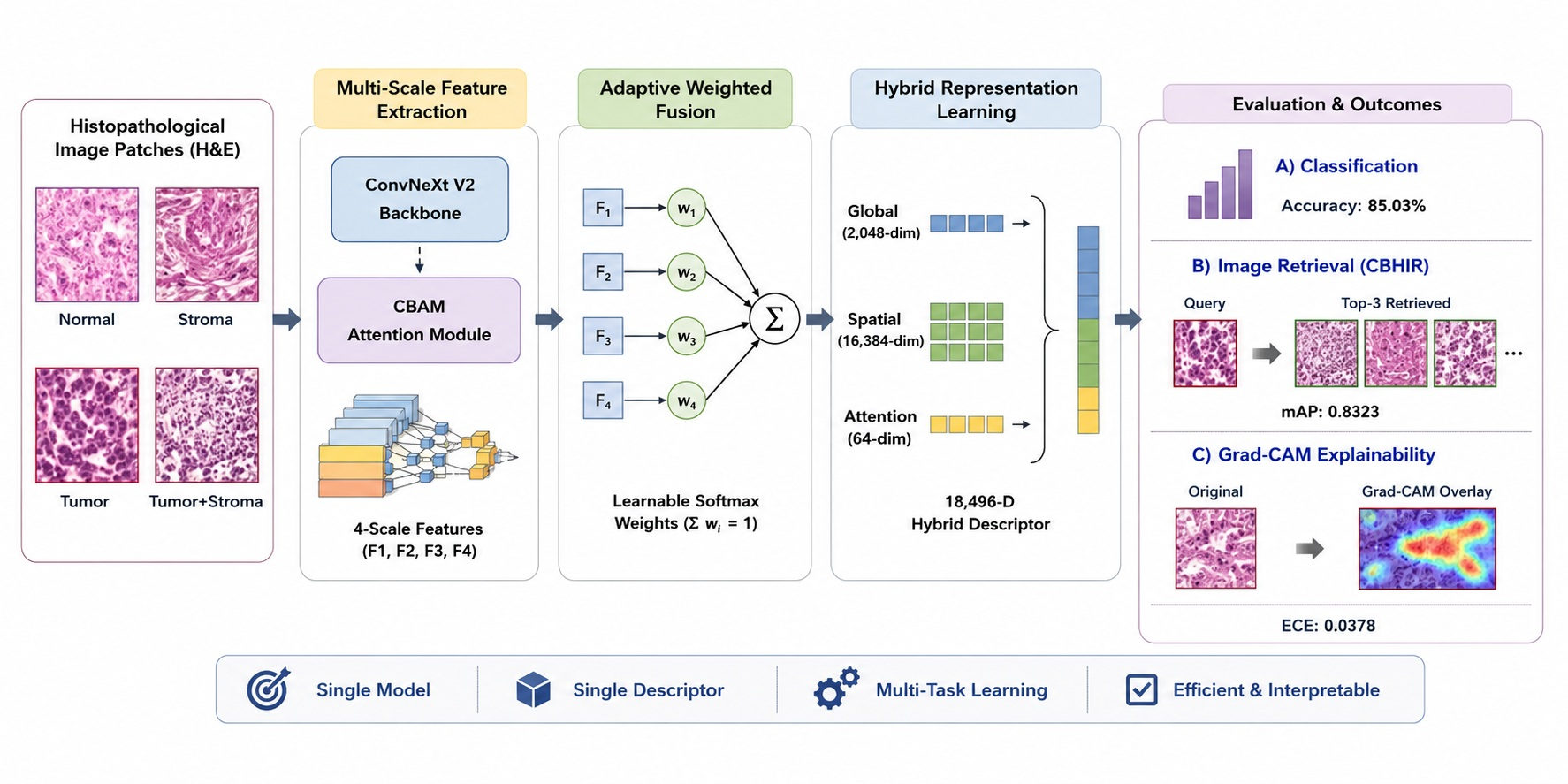
Accurate classification and efficient retrieval of histopathological images are essential for the diagnosis of lung adenocarcinoma (LUAD). Existing deep learning approaches for Content-Based Histopathological Image Retrieval (CBHIR) typically generate single-scale embeddings, missing the richer spatial context from earlier network stages. We propose a unified framework composed of: (1) a ConvNeXt V2 backbone with an integrated Convolutional Block Attention Module (CBAM) for multi-scale feature extraction, (2) an Adaptive Weighted Fusion Neck with learnable softmax-normalized weights, and (3) a novel Hybrid Representation Head producing an 18,496-dimensional descriptor by concatenating global, spatial, and attention-weighted features. Evaluated on the WSSS4LUAD dataset (10,087 patches, four tissue classes), our model achieves 85.03% accuracy (5-fold CV: 83.35 ± 0.93%), F1-score of 0.8116, mean Average Precision (MAP) of 0.8323 for retrieval, and an Expected Calibration Error (ECE) of 0.0378. Ablation experiments confirm that all proposed modules contribute positively, with the Attention Branch being the most impactful (Δ = −2.13%). The framework further provides Gradient-weighted Class Activation Mapping (Grad-CAM) explainability for clinical interpretability.

Graphical Abstract

1. Introduction

Lung cancer remains the leading cause of cancer-related mortality worldwide, and lung adenocarcinoma (LUAD) is its most common histological subtype [1]. Pathological examination of hematoxylin and eosin (H&E)-stained sections is the diagnostic gold standard, but it forces pathologists to analyze whole-slide images (WSIs) that can reach 100,000 × 100,000 pixels at the highest magnification [2]. The large volume of data generated by digital pathology, together with a rising pathologist workload, has driven work on computer-aided diagnostic (CAD) tools [3].
Among the CAD tools proposed for this workload, Content-Based Histopathological Image Retrieval (CBHIR) is now widely used to help pathologists locate visually similar tissue images in large archives for comparison-based diagnosis and teaching [4,5]. Unlike keyword-based search, CBHIR extracts meaningful feature descriptors from images and measures similarity in a learned embedding space [6]. The quality of a CBHIR system therefore depends on the quality of those descriptors.
These descriptor-based systems have been reshaped by deep learning, in particular Convolutional Neural Networks (CNNs) and Vision Transformers (ViTs) [7,8]. Current approaches, however, share two recurring limitations. First, they typically extract features from a single scale—usually the deepest layer—and miss spatial context from earlier layers that captures local structure [9]. Second, models pre-trained on natural-image corpora, such as ImageNet, transfer imperfectly to H&E histopathology because of differences in texture, color distribution, and morphology [10].
Within this line of research, Nuñez-Fernández et al. [11] recently introduced the Local–Global Feature Fusion Embedding Model (LGFFEM), showing that local–global fusion with a Generalized Mean (GeM) head reaches state-of-the-art retrieval on Kimia Patch24C ( η p = 99.40%). Their ConvNeXt V2 + BiFPN-style backbone targets retrieval only, which limits its use as an end-to-end diagnostic tool.
To close these gaps, we propose a unified framework that performs classification and retrieval in a single pass. The framework contributes:
  • Hybrid Representation Head: A novel three-branch architecture that produces an 18,496-dimensional feature descriptor by concatenating global semantic features (2048-dim), spatial layout features (16,384-dim), and attention-weighted features (64-dim), capturing complementary information at different abstraction levels.
  • Adaptive Weighted Fusion Neck: A multi-scale feature aggregation module that uses learnable softmax-normalized weights to combine features in a manner that is adaptive to the data.
  • Comprehensive Evaluation Framework: A single system that is assessed on the WSSS4LUAD lung adenocarcinoma dataset with classification metrics, retrieval metrics (MAP, MRR, P@K, NDCG@K), and medical accuracy metrics ( η p , η w , η tot ), calibration analysis (ECE), and Grad-CAM explainability.
  • Dual-Purpose Architecture: This is a general architecture that can be customized to perform both tissue classification with calibrated probabilities and content-based image retrieval, evaluated by means of a comprehensive set of metrics, including medical accuracy, calibration analysis (ECE), and Grad-CAM explainability for clinical interpretability.
While the individual building blocks we adopt—ConvNeXt V2, the Convolutional Block Attention Module (CBAM), multi-scale feature fusion, Grad-CAM, and learned retrieval descriptors—have each appeared in prior medical-imaging work, the specific novelty of this study is their unification into a single descriptor that simultaneously supports classification and retrieval. Concretely, our contribution is threefold: (i) an Adaptive Weighted Fusion Neck whose four softmax-normalized scale weights are fully learnable end-to-end, rather than the fixed or fast-normalized fusion patterns of BiFPN-style necks; (ii) an 18,496-dimensional Hybrid Representation Head that explicitly concatenates global semantic, dense spatial-layout, and attention-weighted features so that the same vector drives both a calibrated classifier and a FAISS retrieval index; and (iii) a unified, single-pass design in which classification, retrieval, calibration, and explainability are obtained from one forward pass and one descriptor, whereas prior CBHIR models, such as LGFFEM, are retrieval-only. To our knowledge, this combination has not been reported for lung adenocarcinoma histopathology.
Beyond classification, the content-based retrieval component is intended to serve concrete clinical roles. By returning visually and morphologically similar LUAD patches from an indexed archive, the system can act as a diagnostic aid that surfaces previously confirmed cases for side-by-side comparison, support case-based reasoning for ambiguous or borderline regions, assist trainee education by retrieving canonical examples of each tissue pattern, help recognize rare or atypical patterns by matching them against the archive, and contribute to quality control by flagging when a query is dissimilar to any confidently labeled exemplar. In this work, retrieval is positioned as a similarity-search and secondary-verification tool that complements—rather than replaces—the pathologist’s judgment.
The remainder of this paper is organized as follows. Section 2 reviews related work on content-based histopathological image retrieval, multi-scale feature fusion, attention mechanisms, and modern convolutional backbones. Section 3 details the proposed method, including the ConvNeXt V2–CBAM backbone, the Adaptive Weighted Fusion Neck, the Hybrid Representation Head, the classifier, and the loss function. Section 4 describes the datasets, implementation details, and evaluation protocol. Section 5 reports and analyzes the classification, retrieval, calibration, ablation, and explainability results. Section 6 discusses the findings and limitations, and Section 7 concludes with directions for future work.

2. Related Works

This section situates our work within four lines of research that directly inform the proposed framework. We first review content-based histopathological image retrieval (Section 2.1), which motivates the need for discriminative image descriptors; we then survey multi-scale feature fusion (Section 2.2) and attention mechanisms for medical imaging (Section 2.3), which underpin our neck and backbone designs, respectively; and we close with modern convolutional backbones (Section 2.4), which justify our choice of ConvNeXt V2. For each line we highlight the gap that our unified classification-and-retrieval design is intended to fill.

2.1. Content-Based Histopathological Image Retrieval

Contemporary CBHIR systems are designed based on the use of deep learning models to extract image descriptors embeddings. Hegde et al. [4] suggested a CNN-based image search tool, SMILY, which uses multi-similarity loss to train the tool. Yang et al. [12] implemented a mixed-attention mechanism, which combined spatial and channel attention with squeeze-and-excitation blocks, and was trained on the Kimia Path24C dataset using multi-similarity loss.
Tabatabaei et al. [13] utilized a Convolutional Auto-Encoder with unsupervised training to extract image descriptors from the bottleneck layer. Mohammad Alizadeh et al. [14] proposed a Siamese CNN hashing model using contrastive pair loss for histopathology image retrieval, addressing imbalanced classes in datasets, such as Kather [15] and BreakHis [16]. Tabatabaei et al. [17] presented a Siamese content-based search engine trained with contrastive loss for skin and breast cancer diagnosis.

2.2. Multi-Scale Feature Fusion

Multi-scale feature extraction has been extensively studied in object detection and segmentation. Feature Pyramid Networks (FPN) [18] introduced a top-down pathway for constructing multi-scale feature maps. BiFPN [19] extended this with bidirectional cross-scale connections and fast normalized fusion weighting. Iqbal and Qureshi [20] proposed a Global-Local Pyramid Pattern for fusing textural and visual features across medical image domains.
Most recently, Nuñez-Fernández et al. [11] proposed LGFFEM, which incorporates a Local-Global Feature Fusion Neck (LGFFN) inspired by BiFPN, using Local and Global Feature Aggregators with channel attention. Their model revealed that the multi-scale fusion enhances the performance of retrieval. We extend this body of work by introducing an adaptive weighted fusion mechanism whose weights are learnable, and a hybrid representation head to perform both classification and retrieval.

2.3. Attention Mechanisms for Medical Imaging

Attention mechanisms have been shown to be useful in concentrating neural networks on diagnostically significant areas. Channel attention was proposed by Squeeze-and-Excitation (SE) networks [21], which used global average pooling and a bottleneck MLP. Convolutional Block Attention Module (CBAM) [22] that builds on SE introduced sequential channel and spatial attention, which showed to be more effective in image recognition tasks. Shao et al. [23] demonstrated that global characteristics along with attention-based re-ranking are capable of providing good performance in image retrieval.

2.4. ConvNeXt V2 and Modern CNN Architectures

ConvNeXt V2 [24] is an updated CNN design that embraces the design philosophy of Vision Transformers, whilst preserving the efficiency of convolutional operations. The Global Response Normalization (GRN) layer, which normalizes features using a global context to encourage diversity of features across channels, and a training paradigm based on masked autoencoders, are key innovations. ConvNeXt V2 has demonstrated competitive performance with ViTs on a variety of benchmarks and has favorable computational properties for medical imaging applications.

3. Proposed Method

This section presents the proposed framework in full. We begin with the clinical and technical motivation (Section 3.1), then give an overview of the four-component pipeline (Section 3.2). The subsequent subsections describe each component in turn: the ConvNeXt V2 backbone with CBAM attention (Section 3.3), the Adaptive Weighted Fusion Neck (Section 3.4), the Hybrid Representation Head (Section 3.5), and the classifier (Section 3.6), followed by the training objective (Section 3.7). Throughout, we explain how each module contributes to both tissue classification and content-based retrieval from a single shared descriptor.

3.1. Motivation

In the histopathology of lung adenocarcinoma, the tissue classification method requires the identification of patterns at different spatial resolutions: cellular morphology at fine scales, tissue architecture at intermediate scales, and structural organization at coarse scales. The four LUAD tissue classes—normal alveolar tissue, stromal connective tissue, tumor epithelial tissue, and tumor-associated stroma—share an overlapping visual appearance, so single-scale contextual reasoning is insufficient.
In addition to classification, a clinical support system must also retrieve similar past cases for comparison-based diagnosis and provide explainable visualizations that instill confidence in the clinician. These needs influence our design: a single multi-scale system with hybrid feature representations, as outlined in the rest of this section.

3.2. Overall Architecture

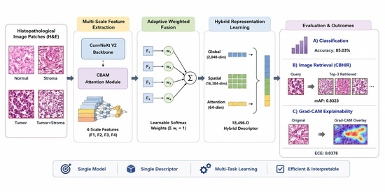
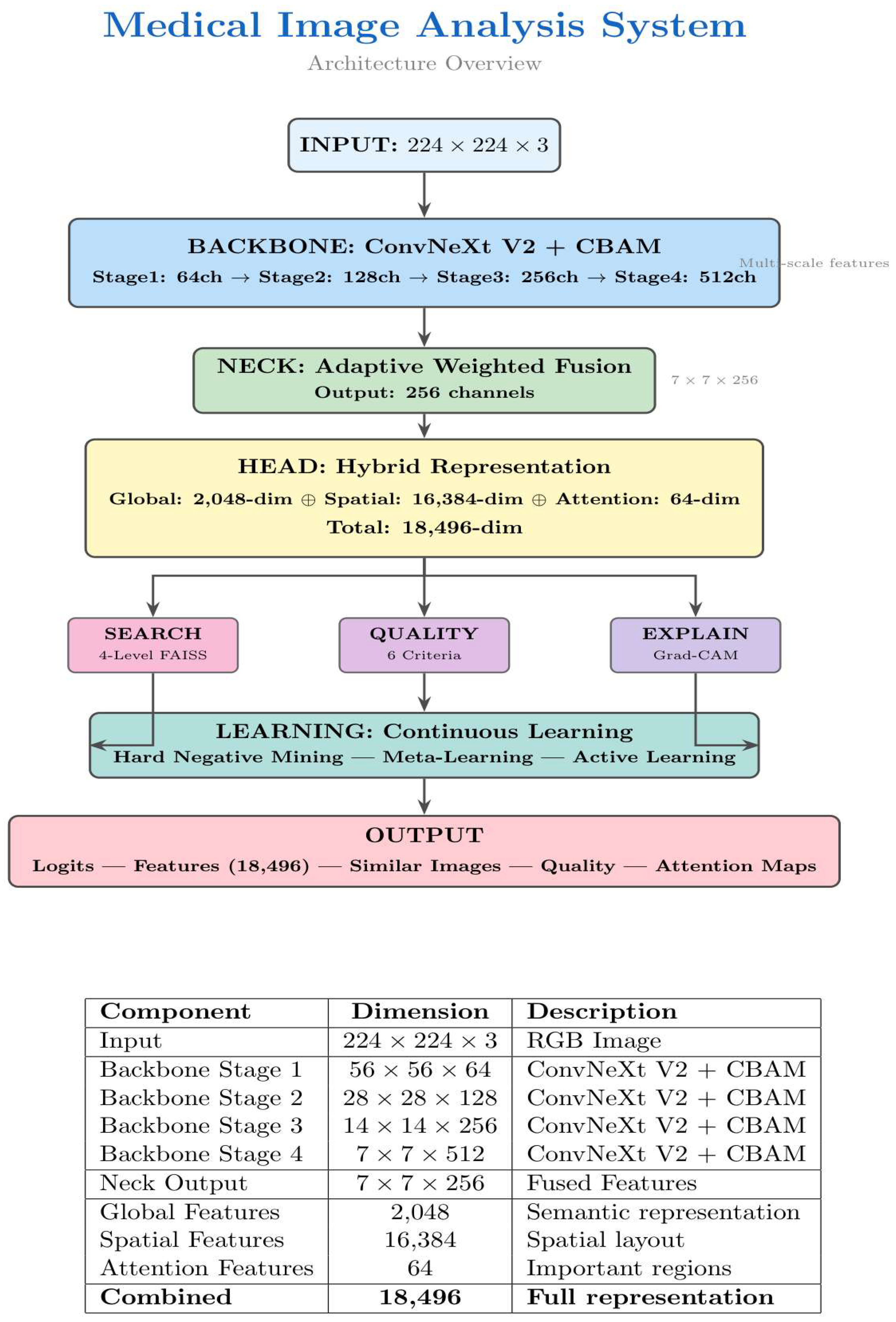
The proposed framework consists of four principal components arranged in a sequential pipeline, as illustrated in Figure 1:
  • Backbone: A ConvNeXt V2 network with integrated CBAM attention modules for multi-scale feature extraction from four stages.
  • Neck: An Adaptive Weighted Fusion module that aggregates multi-scale features using learnable softmax-normalized weights.
  • Head: A Hybrid Representation module that produces a rich 18,496-dimensional feature descriptor through three complementary branches.
  • Classifier: A lightweight neural network that maps the feature descriptor to class probabilities.
Figure 1. Overall architecture of the proposed framework. The input image is processed by a ConvNeXt V2 backbone with CBAM attention to produce multi-scale features { F 1 , F 2 , F 3 , F 4 } . The Adaptive Weighted Fusion Neck aggregates these features using learnable softmax weights. The Hybrid Representation Head produces an 18,496-dimensional descriptor through three branches: global (2048-dim), spatial (16,384-dim), and attention-weighted (64-dim). The descriptor is used for both classification and FAISS-based retrieval.
Computers 15 00473 g001
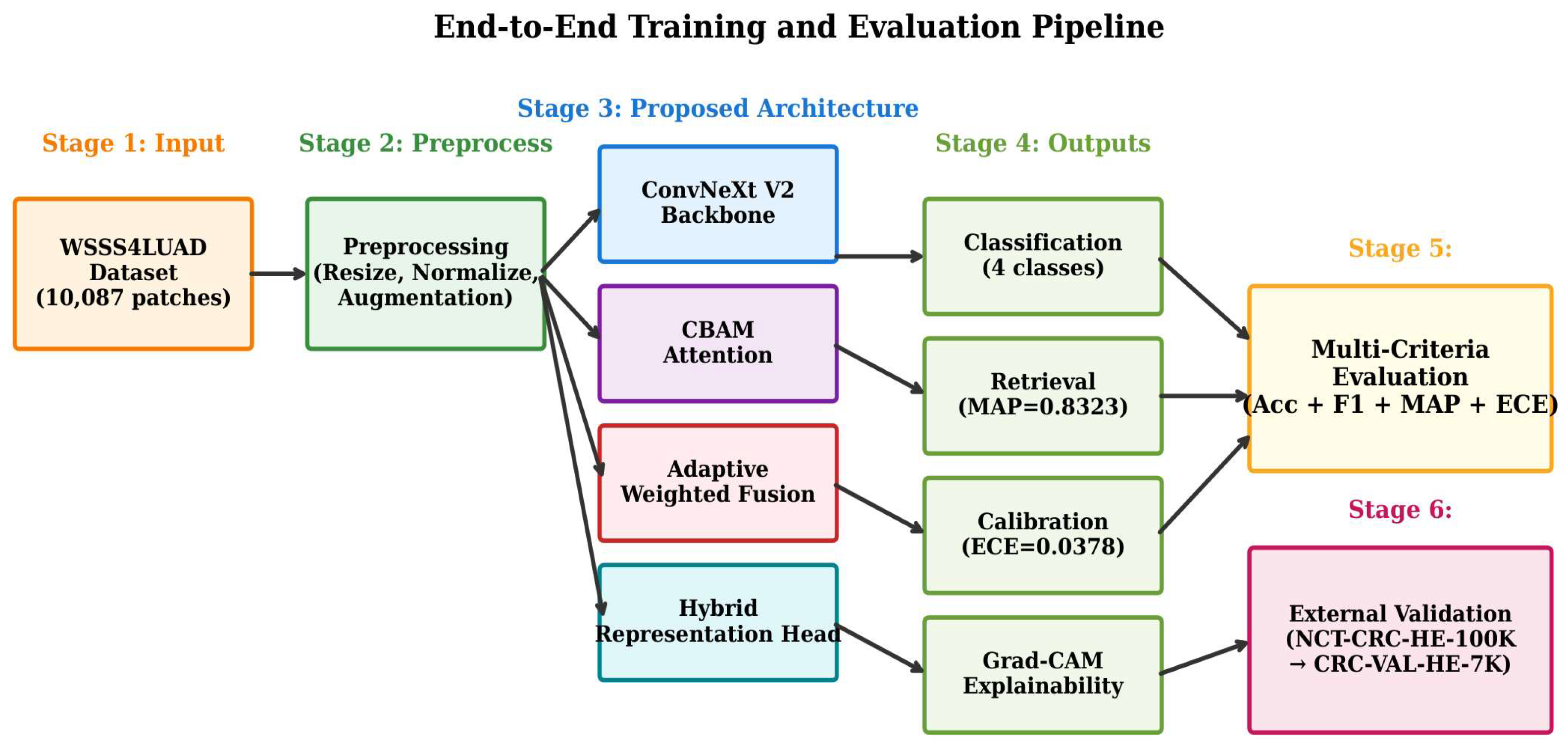
The feature descriptor from the Head serves dual purposes: it is used by the Classifier for tissue classification and by a FAISS-based index for content-based image retrieval. The complete end-to-end training and evaluation pipeline of the proposed framework is illustrated in Figure 2.

3.3. Backbone: ConvNeXt V2 with CBAM Attention

We employ ConvNeXt V2 [24] as our backbone network, configured with four stages of depths [2, 2, 6, 2] and channel dimensions [64, 128, 256, 512]. The network processes an input image of size 224 × 224 × 3 through a stem layer (4 × 4 convolution with stride 4) followed by four hierarchical stages, producing feature maps at progressively lower spatial resolutions.
Each ConvNeXt V2 segment includes a transformation by depth (7 × 7 kernel), layer normalization, inverse stem expansion (4×), and a global response normalization (GRN) layer. The GRN layer, unique to ConvNeXt V2, normalizes features based on their global l 2 statistics:
GRN X = γ · X · X 2 mean X 2 + ϵ + β + X
where γ and β are learnable parameters and · _2 denotes the l_2 norm across spatial dimensions. This normalization promotes feature diversity across channels, which is useful for capturing images of the different morphological styles present in histopathological images.
We integrate the Convolutional Block Attention Module (CBAM) [22] after each backbone stage to enhance feature representation through sequential channel and spatial attention.
  • Channel Attention:
M c F = σ   MLP AvgPool F + MLP MaxPool F
where σ is the sigmoid function, MLP is a shared multi-layer perceptron with a reduction ratio of 16, and AvgPool and MaxPool are global pooling operations.
  • Spatial Attention:
M s F = σ   Conv 7 × 7   AvgPool c F ; MaxPool c F
where AvgPool c and MaxPool c operate across the channel dimension, and Conv 7 × 7 is a 7 × 7 convolution.
The CBAM-enhanced feature at stage i is computed as:
F ^ i = M s F i F i , where F i = M c F i F i  
The backbone produces four CBAM-enhanced feature maps: F ^ 1 R 64 × H 4 × W 4 , F ^ 2 R 128 × H 8 × W 8 , F ^ 3 R 256 × H 16 × W 16 , and F ^ 4 R 512 × H 32 × W 32 .

3.4. Neck: Adaptive Weighted Fusion

Unlike the BiFPN-inspired architecture in LGFFEM [11], which uses multiple aggregation nodes with fixed fusion patterns, we propose a simpler yet effective Adaptive Weighted Fusion mechanism with fully learnable weights.
Lateral Projections. Each backbone feature map is first projected to a common channel dimension C out = 256 using 1 × 1 convolutions:
L i = GELU   BN   Conv 1 × 1 ( F ^ i ) , i 1 , 2 , 3 , 4
Adaptive Fusion. All projected features are resized to a common spatial resolution ( H 32 × W 32 ) using bilinear interpolation, then combined using learnable weights:
w = softmax w 1 , w 2 , w 3 , w 4
F fused = i = 1 4 w i · Resize L i
The softmax normalization ensures that the fusion weights are non-negative and sum to one, providing an interpretable measure of each scale’s contribution. During training, the model learns to assign higher weights to the most informative scales for the specific dataset and task.
Implementation and interpretation of the learned weights. The fusion weights are a single learnable vector w = [w_1, w_2, w_3, w_4] that is optimized jointly with all other network parameters by back-propagation of the classification loss; no auxiliary supervision is applied to them. Equation (6) maps the four raw logits to a probability simplex through the softmax, and Equation (7) applies them to the four lateral-projected, spatially-aligned feature maps. The weights are global (shared across all images) and are therefore fixed after training; they are not predicted per sample. On WSSS4LUAD, the converged weights are w_1 = 0.232 (stage 1, 1/4 resolution), w_2 = 0.262 (stage 2, 1/8), w_3 = 0.287 (stage 3, 1/16), and w_4 = 0.218 (stage 4, 1/32). The distribution is relatively flat—every scale receives 22–29% of the weight—which shows that no single resolution dominates and confirms that genuinely multi-scale information is exploited. The largest weight is assigned to the intermediate stage (stage 3), consistent with mid-level tissue-architecture cues being the most discriminative for the four LUAD classes, while the coarsest stage (stage 4) receives the smallest weight.
Output Refinement. The fused feature map is refined through a 3 × 3 convolution:
F neck = GELU   BN   Conv 3 × 3 ( F fused )
where F neck R 256 × 7 × 7 is the output of the neck module for a 224 × 224 input.

3.5. Head: Hybrid Representation

Inspired by the observation that different types of information are encoded at different spatial granularities, we design a three-branch Hybrid Representation Head that captures complementary features.
Branch 1—Global Features ( f g R 2048 ): Global features capture holistic semantic information through adaptive average pooling:
f g = Dropout GELU LN W g · GAP ( F neck ) + b g
where GAP is global adaptive average pooling, W g R 2048 × 256 is a linear projection, LN is layer normalization, and the dropout rate is 0.1.
Branch 2—Spatial Features ( f s R 16384 ): Spatial features preserve the layout information through grid pooling at an 8 × 8 resolution:
f s = Dropout GELU LN W s · Flatten ( GP 8 × 8 ( F neck ) ) + b s
where GP 8 × 8 performs adaptive average pooling to an 8 × 8 spatial grid, producing a 256 × 8 × 8 = 16,384 -dimensional vector after flattening. This branch preserves the spatial distribution of features. This branch facilitates the extraction of the structural patterns characteristic of tissue architecture.
Branch 3—Attention-Weighted Features ( f a R 64 ): Attention- based features highlight the most diagnostically relevant regions through a learned attention mechanism:
A = σ Conv 1 × 1 GELU Conv 1 × 1 ( F neck )
f a = Dropout GELU LN GAP Conv 1 × 1 ( F neck ) A
where A R 1 × H × W denotes a spatial attention map that assigns importance weights to individual spatial locations.
Feature Concatenation. The final image descriptor is formed by concatenating all three branches:
f = f g ; f s ; f a R 18496
where 18,496 = 2048 + 16,384 + 64 . The spatial features constitute the dominant component at 88.6% of the total dimensionality, reflecting the critical importance of preserving spatial layout information for histopathological analysis, where tissue architectures differ primarily in structural organization. The global features (11.1%) capture holistic semantic content, while the compact attention-weighted features (0.3%) provide a focused signal highlighting diagnostically relevant regions. This asymmetric design is intentional: the high spatial dimensionality enables fine-grained retrieval of structurally similar tissue patterns. The descriptor serves both for classification (through the classifier head) and for retrieval (through FAISS indexing).
Justification of the descriptor size and the accuracy–efficiency trade-off. The 18,496-dimensional descriptor is a deliberate design choice rather than an arbitrarily large embedding. The dimensionality is fully determined by the architecture: the 8 × 8 grid-pooled spatial branch yields 256 × 8 × 8 = 16,384 values, the global branch 2048, and the attention branch 64. We retain the full spatial branch because, unlike object-centric natural images, histopathological classes are distinguished mainly by the spatial arrangement of glands, stroma, and epithelium; aggressive pooling of this branch removes exactly the layout cues that the retrieval task relies on, as confirmed by the ablation in which removing the spatial branch lowers accuracy (Section 5.3). In terms of cost, each descriptor occupies roughly 72 KB in float32, so the entire 8070-patch training archive requires under 0.6 GB and is indexed with FAISS IVFFlat (100 clusters, 10 probes) with sub-millisecond query latency on a single GPU; storage and search are therefore not bottlenecks at this dataset scale. Nevertheless, for very large or whole-slide archives the descriptor can be compressed without retraining the backbone—e.g., by PCA or product-quantization of the spatial branch, by binary hashing for approximate search, or by learning a compact projection head—and a systematic study of this accuracy-versus-compactness trade-off is identified as future work (Section 6 and Section 7).

3.6. Classifier

The classification head maps the 18,496-dimensional descriptor to class probabilities:
y ^ = W 2 · Dropout GELU LN W 1 f + b 1 + b 2
where W 1 R 512 × 18496 and W 2 R 4 × 512 . Layer normalization and GELU activation provide non-linearity, while dropout (rate 0.1) prevents overfitting.

3.7. Loss Function

We train the model using cross-entropy loss with label smoothing:
L = c = 1 C q c l o g p c
where q c = ( 1 ε ) · y c + ε / C is the smoothed target distribution, y c is the one-hot encoded ground truth, p c is the predicted probability for class c , C = 4 is the number of classes, and ε = 0.05 is the smoothing parameter. Label smoothing prevents overconfident predictions and improves model calibration, which is particularly important in clinical applications.

4. Experiments

4.1. Dataset: WSSS4LUAD

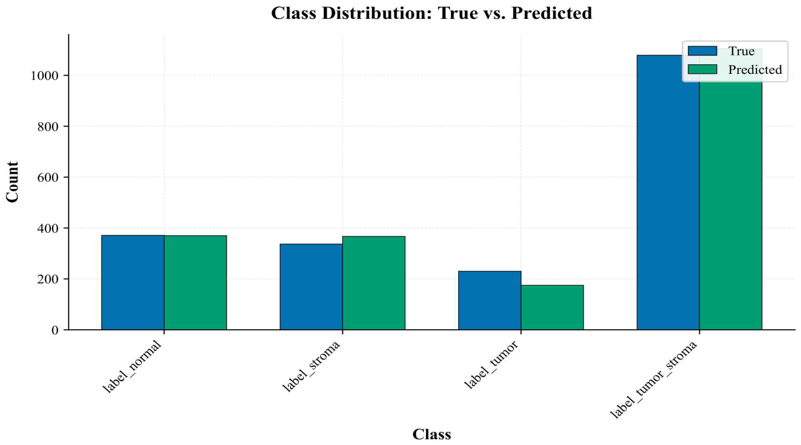
We evaluate our framework on the WSSS4LUAD dataset [25], a publicly available benchmark for lung adenocarcinoma histopathology. The dataset consists of 10,087 H&E-stained patches extracted from 67 whole-slide images, organized into four tissue classes. The class distribution is shown in Table 1 and visualized in Figure 3.
The dataset exhibits significant class imbalance, with Tumor-Stroma comprising over half of all samples and Tumor being the least represented class. All patches are resized to 224 × 224 pixels for model input. We use an 80/20 random split (seed = 42), giving 8070 training and 2017 validation patches.
Dataset protocol and tissue-class definitions. WSSS4LUAD is a public Grand-Challenge benchmark of hematoxylin-and-eosin (H&E)-stained lung-adenocarcinoma tissue digitized from whole-slide images. The 10,087 image-level patches we use are organized into four tissue categories: Normal (healthy alveolar tissue, 1832 patches, 18.16%), Stroma (tumor-free connective/supporting tissue, 1680 patches, 16.66%), Tumor (malignant adenocarcinoma epithelium, 1181 patches, 11.71%), and Tumor-Stroma (mixed regions containing both tumor epithelium and tumor-associated stroma, 5394 patches, 53.48%). All patches are H&E-stained and standardized to 224 × 224 pixels; per-channel ImageNet normalization is applied, and the color augmentation described in Section 4.4 is used during training to reduce sensitivity to staining variation. The patches originate from 67 whole-slide images released by the challenge organizers.
Regarding data leakage, we acknowledge an important limitation of the present protocol: because the public release provides image-level patches rather than slide identifiers for every patch, our 80/20 split is performed at the patch level rather than the patient or slide level. Patch-level splitting can in principle allow patches from the same slide to appear in both the training and validation sets, which may optimistically bias performance in histopathology. We mitigate this by (i) reporting 5-fold stratified cross-validation (Section 4.7), which shows low variance (83.35 ± 0.93%) and therefore limited split sensitivity, and (ii) evaluating cross-organ generalization on a fully held-out external dataset (CRC-VAL-HE-7K, Section 5.5) whose slides never appear in training. A strict slide-level or patient-level split is identified as important future work, and we explicitly flag this point in the limitations (Section 7).

4.2. Datasets Comparison

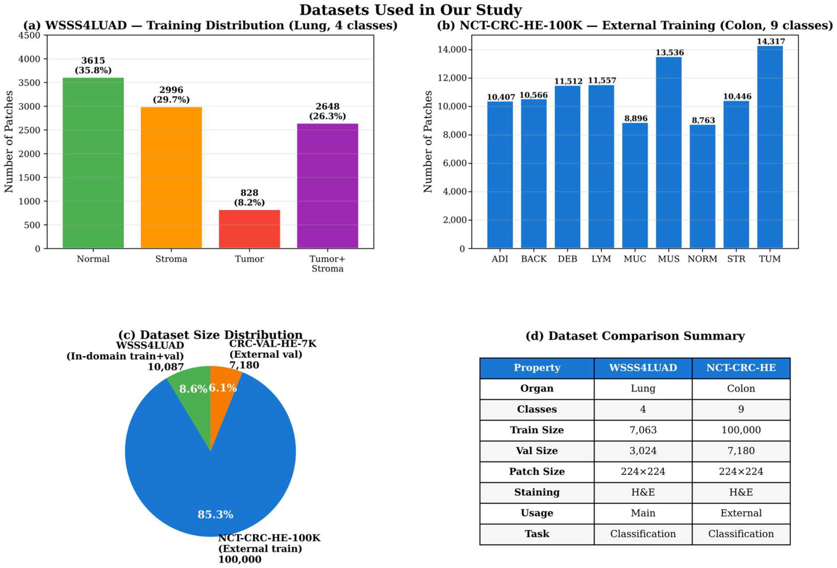
We employ two complementary datasets in our study: WSSS4LUAD as the primary in-domain benchmark and NCT-CRC-HE-100K for external cross-organ validation. Table 2 provides a side-by-side comparison of their key properties.
As Table 2 shows, the two datasets are complementary: WSSS4LUAD is utilized to develop and optimize the proposed architecture on a moderately sized, class-imbalanced four-class lung-tissue dataset. In contrast, NCT-CRC-HE-100K is employed as an external benchmark, characterized by a different organ domain (colon vs. lung), a large number of classes (nine vs. four), and substantially greater scale (approximately ten times more training patches). This combination allows us to test both fine-grained classification ability on the main task and cross-organ transferability of the learned representations. Figure 4 provides an overview of the datasets used in our study.

4.3. Implementation Details

Our framework is implemented in PyTorch 2.7.0 and Torch version 0.22.0. The ConvNeXt V2 backbone is initialized with ImageNet pre-trained weights [24]. We use the AdamW optimizer [27] with an initial learning rate of 1 × 10 4 , weight decay of 0.01, and a cosine annealing learning rate schedule with 5 warmup epochs (linear warmup from 1 × 10 7 ) and a minimum learning rate of 1 × 10 6 . Training is conducted for 150 epochs with a batch size of 16 using mixed-precision training (AMP). The total number of trainable parameters is 287.96 M, with the majority residing in the ConvNeXt V2 backbone and the spatial branch of the Hybrid Representation Head. While the model size is substantial compared to lightweight architectures, such as LGFFEM (14.5 M parameters) [11], the use of mixed-precision training (AMP) reduces GPU memory requirements. Training is performed on an NVIDIA GeForce RTX 5070 Laptop GPU, requiring approximately 240.6 min. Future work will explore knowledge distillation and architectural pruning to reduce computational requirements for resource-constrained clinical deployment.
For image retrieval, we employ the FAISS library [28] with an IVFFlat index (100 clusters, 10 probes) using the 18,496-dimensional feature descriptors. The retrieval evaluation uses the validation set as the query set and the training set as the database.

4.4. Data Augmentation

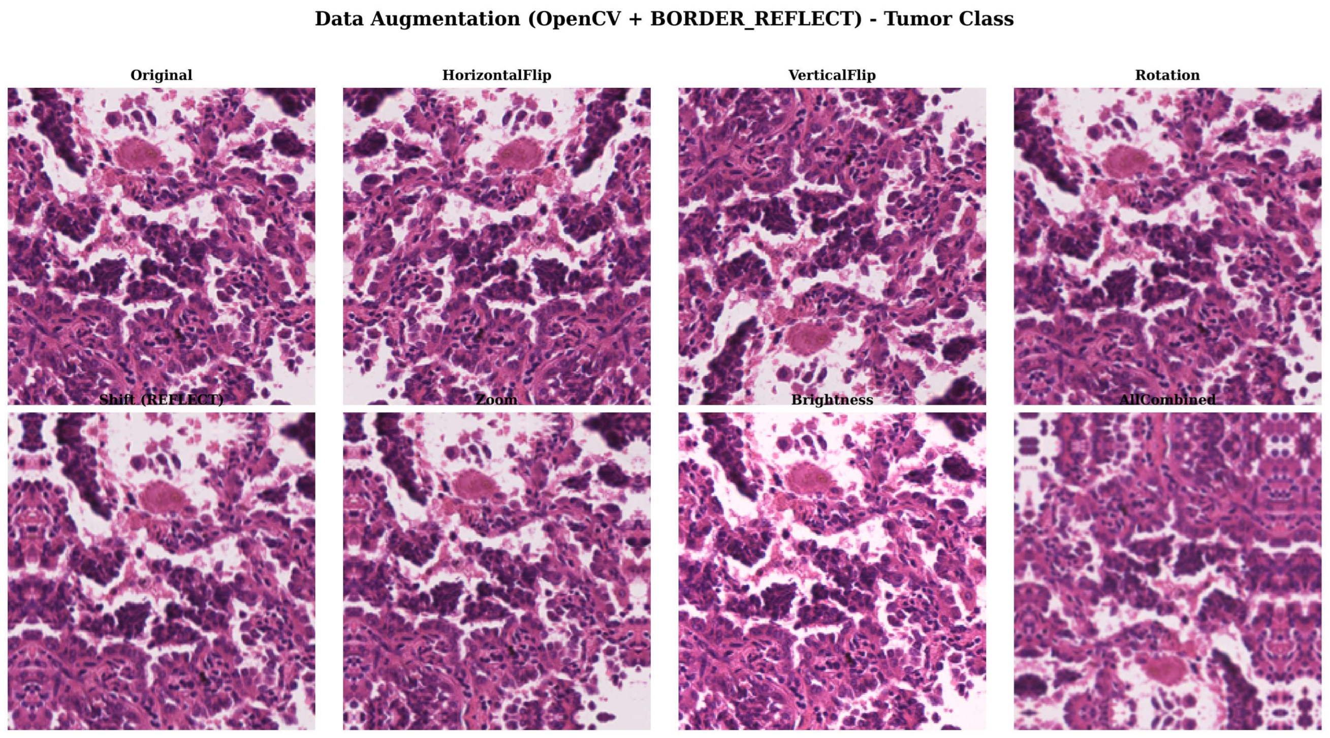
Training images are augmented with the following transformations, as illustrated in Figure 5:
  • Geometric: rotation ( ± 15 ), horizontal and vertical flips (50% probability each), translation ( ± 10 % ), zoom ( 0.9 1.1 × ).
  • Color: brightness, contrast, and saturation jitter ( ± 15 % each in HSV color space).
  • Regularization: random erasing (15% probability, 2–10% of image area).
  • Normalization: ImageNet mean [ 0.485,0.456,0.406 ] and standard deviation [ 0.229,0.224,0.225 ] .
Figure 5. Examples of data augmentation applied to training images. Augmentations include geometric transformations (rotation, flipping, translation), color jitter, and random erasing.
Computers 15 00473 g005
Validation images undergo only resizing and normalization without augmentation.

4.5. Evaluation Metrics

We report the following metrics:
  • Classification: Accuracy, Precision, Recall, F1-score (macro and weighted), Cohen’s kappa ( κ ), Matthews Correlation Coefficient (MCC), balanced accuracy.
  • Medical accuracy [29]: patch-level accuracy η p , whole-scan accuracy η w , and total accuracy η tot = η p × η w .
  • Retrieval: Mean Average Precision (MAP), Mean Reciprocal Rank (MRR), Precision@K, Recall@K, NDCG@K.
  • Calibration: Expected Calibration Error (ECE), Brier score.
  • Explainability: Grad-CAM visualizations on the last backbone stage.

4.6. Cross-Validation Analysis

We perform a 5-fold stratified cross-validation experiment to test the statistical robustness and rule out split-dependent bias. For the full model, each fold is trained separately with the same hyperparameters. Results per-fold and total are given in Table 3.
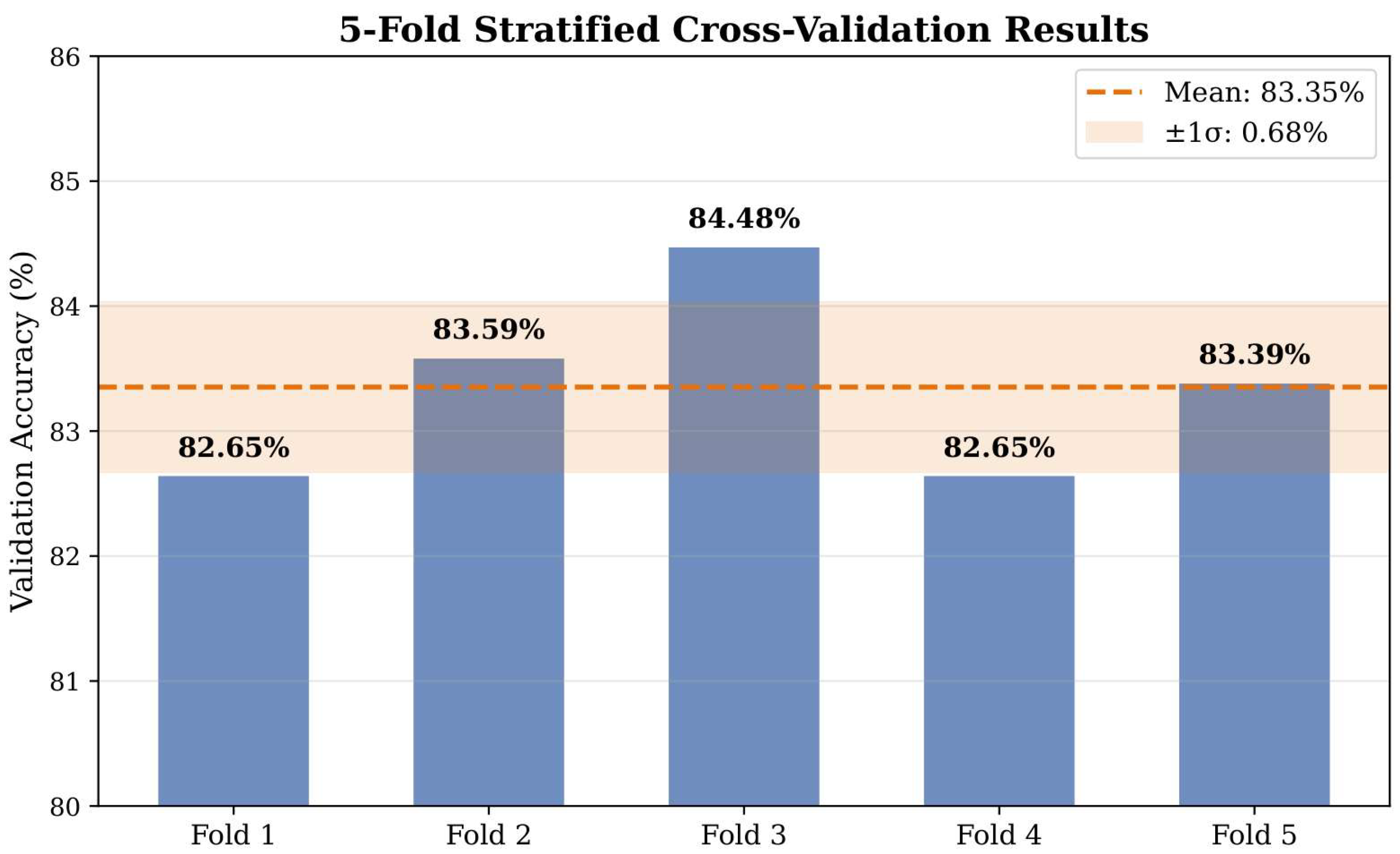
The cross-validation results do not show any instability of the model as the standard deviation of the accuracy across folds (0.93%) is quite low, indicating that the model is not sensitive to the partitioning of the data. Four of the five folds achieve accuracy above 83%, and the mean (83.35%) is very close to the single-split accuracy (85.03%), confirming that the original evaluation is representative of the performance. The results per fold are visualized in Figure 6, along with the mean and ± 1 σ .
The results of the 5-fold stratified cross-validation are shown in Figure 6: The dashed orange line shows the accuracy of 83.35%, the shaded area shows the standard deviation of 0.93%, with high consistency across different data partitions.

4.7. Training Dynamics

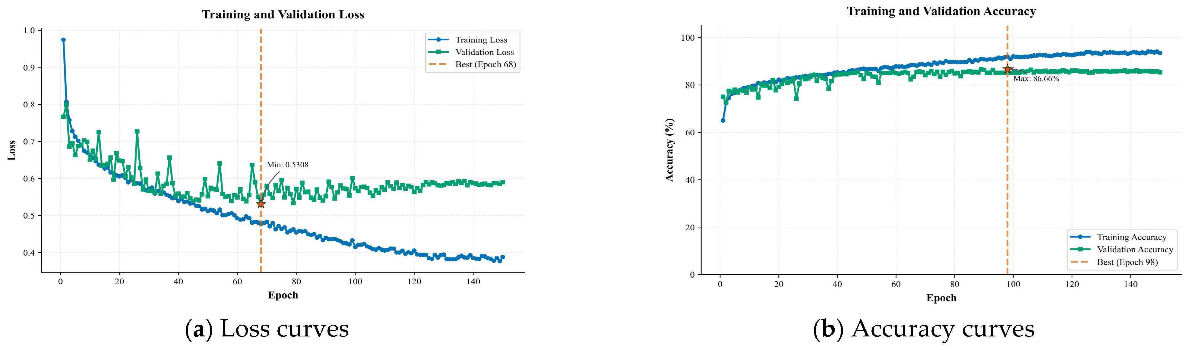
Figure 7 presents the training behavior of the proposed model.
After more than 150 epochs, the model is converging, the training loss is reducing from 0.9745 to 0.3879 and the training accuracy is improving from 64.99% to 93.46%. The validation accuracy is 86.66% at epoch 98, and after that, the validation accuracy fails to improve while the training accuracy keeps rising, suggesting that the model has moderate overfitting. The final generalization gap of ~ 8 percentage points indicates that better regularization techniques or more training data could yield better generalization.
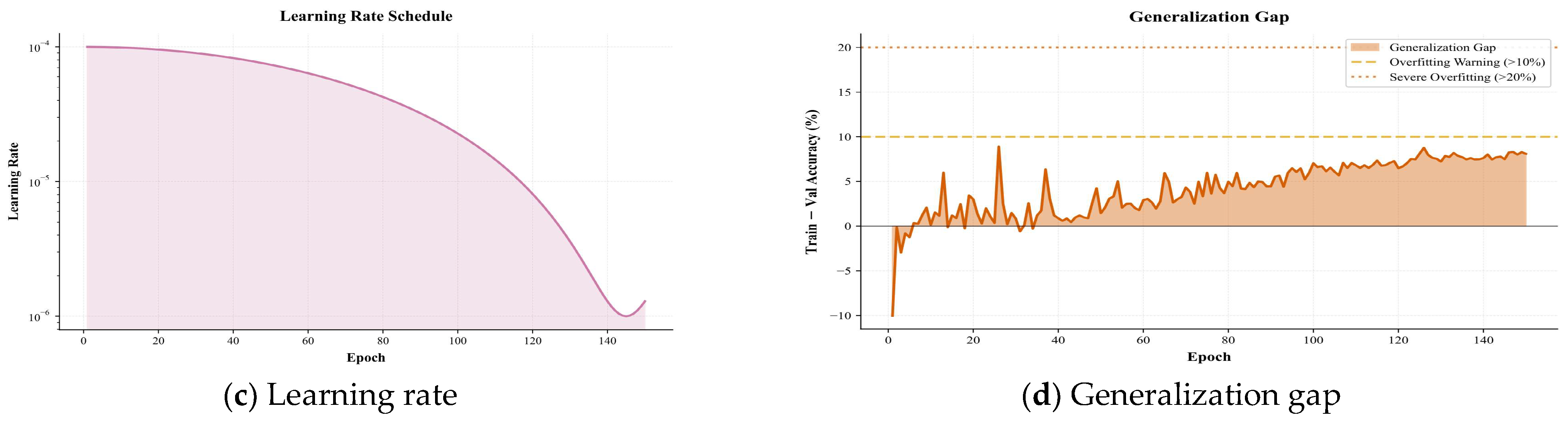
The learning rate decays smoothly with cosine annealing schedule with warmup from 1 × 10 7 in 5 epochs to peak learning rate 1 × 10 4 and slowly goes down to 1 × 10 6 . The generalization gap (the difference between training and validation accuracy) remains at around 7–8% after epoch 100, which indicates that this model has learned its maximum from the dataset it is being trained on, and further increasing the size of the dataset or implementing suitable regularization techniques could further enhance generalization.

5. Results

This section presents the experimental results obtained from the proposed CBHIR framework using multiple evaluation perspectives. The performance of the proposed model was assessed through classification accuracy, retrieval effectiveness, architectural comparisons, computational efficiency, and external validation experiments. In addition, ablation studies and per-class analyses were conducted to investigate the contribution of different model components and evaluate the robustness of the framework across various histopathological categories.

5.1. Classification Performance

The overall classification performance on the WSSS4LUAD validation set is reported in Table 4.

5.2. Comparison with Baseline Architectures

To evaluate the performance of the proposed model, it was compared with four widely-used baseline architectures trained under identical experimental conditions (AdamW optimizer, cosine annealing, lr = 10 4 , AMP, 80/20 split). The results are summarized in Table 5.
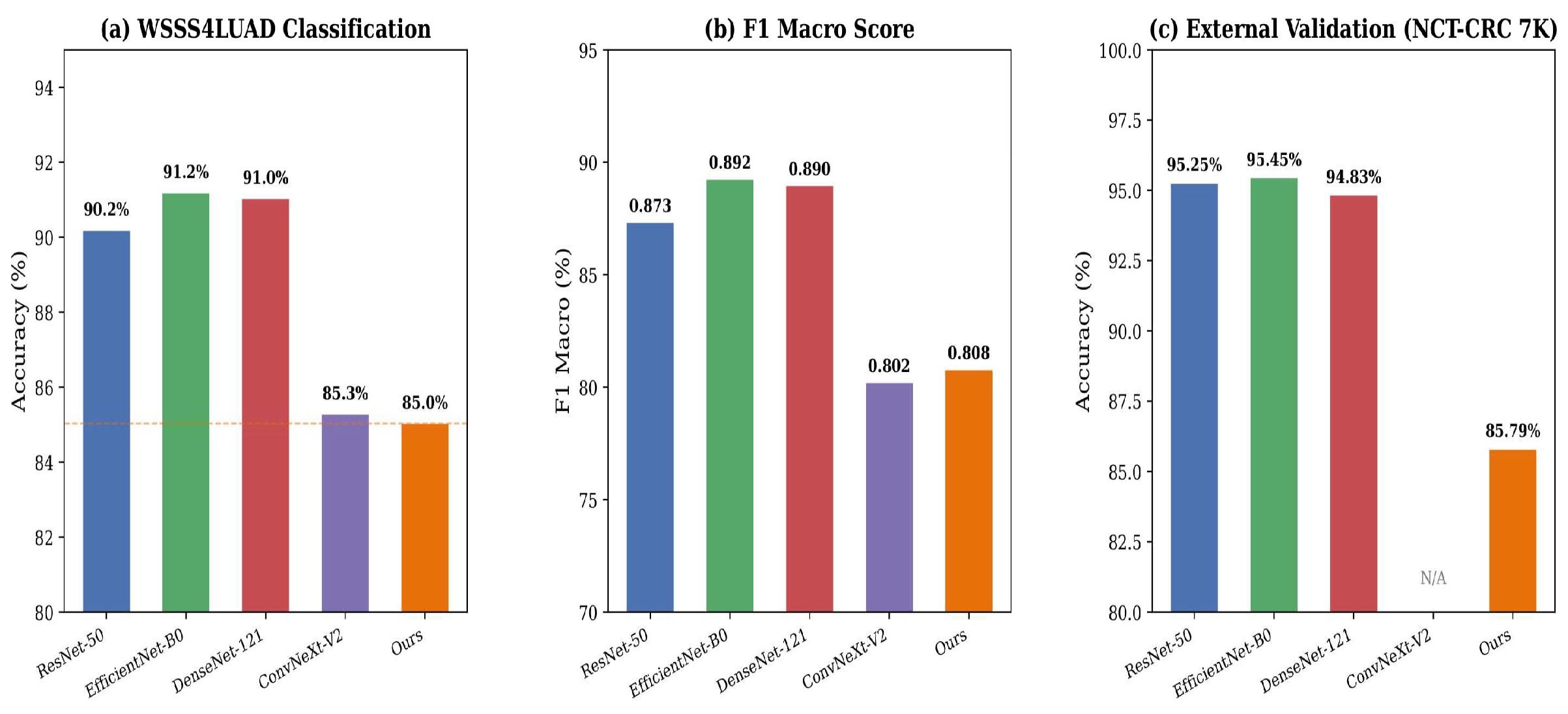
The lightweight models (ResNet-50, EfficientNet-B0, DenseNet-121) perform better on this accuracy (90–91%) than our model (85.03%). The difference is mainly due to our model having a much higher number of parameters: 287.96M as compared to 4.67–24.56M, resulting in some moderate overfitting on the limited training set (8070 samples). Importantly, our proposed Adaptive Fusion Neck and Hybrid Head do not degrade performance, as the vanilla ConvNeXt-V2 backbone is able to achieve 85.28% accuracy. The model proposed here has three benefits: First, it can generate class labels as the baselines do, but also an 18,496-dimensional feature descriptor for content-based retrieval (MAP = 0.8323 , MRR = 0.8784 ), second, it can provide calibrated probabilities (ECE = 0.0378 ), and third, it can provide Grad-CAM explainability—all of which the baselines are missing.
To demonstrate the cross-organ generalization, we compared all the models in Figure 8 by accuracy, F1 macro, and external validation on NCT-CRC-HE-100K CRC-VAL-HE-7K.

5.3. Ablation Study

To show the significance of each proposed component, we perform a systematic ablation study by systematically removing individual components while preserving the remaining architecture. The hyperparameters used in training are the same for all variants. The results are given in Table 6.
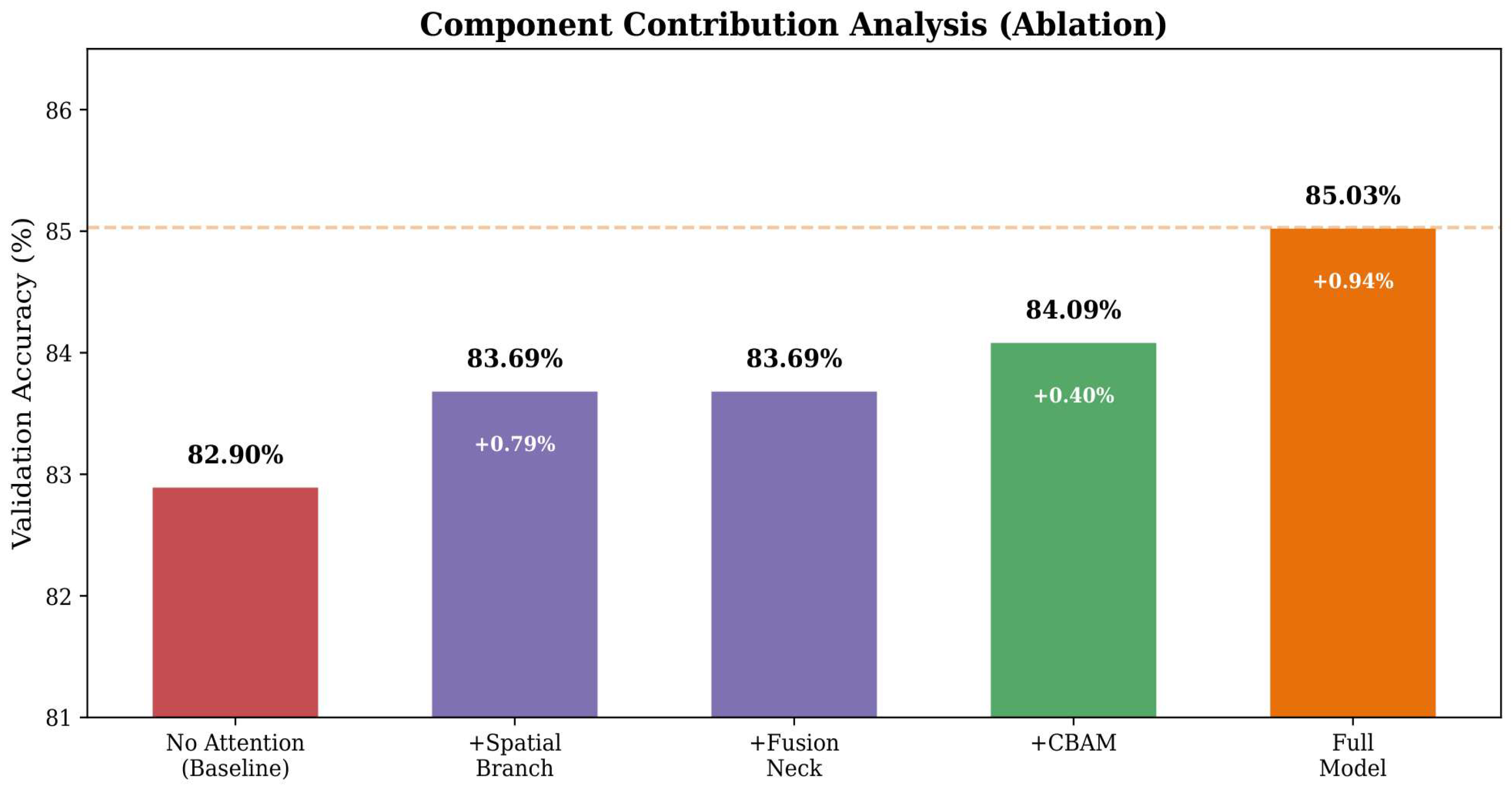
The ablation results reveal several insights. The advantage of all proposed components is positive, in the sense that the accuracy decreases by about 0.94–2.13% when any one of the modules is removed. Second, the most effective component is the Attention Branch ( Δ = 2.13 % , F1 drops from 0.8077 to 0.7477), suggesting that attention weighted features contain discriminative information that is important for the classification task. Third, the smallest contribution comes from the CBAM module ( Δ = 0.94 % ), indicating that some channel–spatial relationship is already picked up in the backbone. Fourth, all the components are complementary, as the combined effect is greater than the sum of its parts, suggesting there is complementary information captured. The layout is well balanced—there is no single module that dominates performance. The incremental contribution of each component is visualized in Figure 9.
To isolate the source of the performance gain, the six configurations in Table 6 progressively decompose the architecture along the axes requested for a thorough ablation. The “Global-features-only” variant approximates the plain backbone-plus-global-pooling baseline (descriptor reduced to 2048-D), removing both the spatial and attention branches; “w/o CBAM” isolates the contribution of the backbone attention; “w/o Adaptive Fusion” replaces the learnable softmax weights with uniform averaging, testing the value of learnable fusion; “w/o Spatial Branch” and “w/o Attention Branch” remove the corresponding head components and, in doing so, reduce the descriptor dimensionality, so they double as lower-dimensional-descriptor variants. Read together, these results show that the gain is not attributable to a single factor: the attention-weighted features contribute most (Δ = −2.13%), the learnable multi-scale fusion and the spatial branch each add roughly 1.3%, and backbone CBAM adds a further 0.9%, with the full model exceeding every reduced variant. A fully factorial study (e.g., backbone-plus-CBAM in isolation and intermediate descriptor sizes obtained by PCA) is left for future work.

5.4. Inference Efficiency

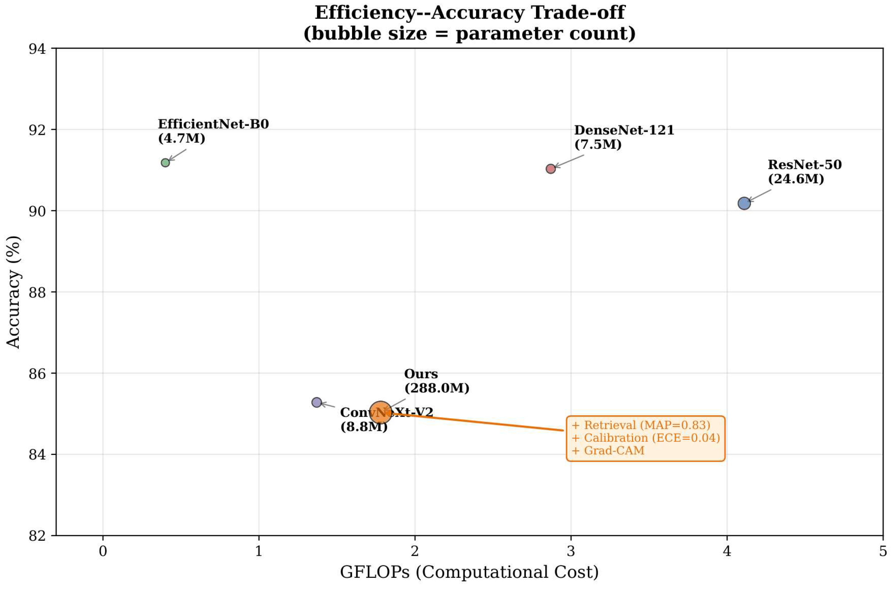
Table 7 shows the computational efficiency of all models evaluated. Even though it has a large number of parameters, the proposed model achieves competitive throughput and the second lowest GFLOPs compared to all architectures, thanks to the efficient ConvNeXt-V2 design.
The efficiency/accuracy trade-off is shown in a bubble chart in Figure 10, with the size of the bubbles indicating the number of parameters used. Even with the largest model size, our framework delivers competitive GFLOPs (1.78) and offers further capabilities (retrieval, calibration, explainability) that are not included in any of the baselines.
The overall agreement between the model and the human experts is 85.03% with Cohen’s kappa of 0.7689, which is considered substantial agreement. If class ordering is taken into account, the agreement level is further improved with a weighted kappa of 0.8841. Of particular interest, the top 3 accuracy is 99.60%, meaning the correct class is very likely to be among the top 3 predictions of the model. The ECE of 0.0378 validates a well-calibrated probability estimate, a key element for reliable clinical decision support.
All reported metrics are at the final model checkpoint (epoch 150). Although the validation accuracy of the best epoch (epoch 98) was 86.66%, the final checkpoint is reported to ensure consistent and reproducible evaluation with all metrics, as discussed in Section 5.5.

5.5. External Dataset Validation

To assess generalizability beyond WSSS4LUAD, we evaluate all architectures on the NCT-CRC-HE-100K colorectal tissue dataset [26], reflecting the rapid adoption of artificial intelligence for colorectal cancer analysis [30]. This benchmark contains 100,000 training patches and a held-out validation set of 7180 patches (CRC-VAL-HE-7K), spanning 9 histologically distinct tissue classes (ADI, BACK, DEB, LYM, MUC, MUS, NORM, STR, TUM). To ensure a scientifically rigorous and fair comparison, all four models—including our proposed architecture—are trained on the same stratified 10.8K subsample of NCT-CRC-HE-100K (1200 images per class, identical random seed), and evaluated on the same CRC-VAL-HE-7K validation set. Each model is trained for up to 10 epochs with early stopping (patience = 4–5) and AdamW optimizer (lr = 1 × 10 4 , weight decay = 0.01).
Table 8 presents the fair comparison where all models are trained on the same 10.8 K subsample. Under the same experimental setting, the three lightweight baselines get an accuracy of 94.83–95.45%, which are higher than our model achieving 85.79%, with a gap of 9.66%. This is a more scientifically valid comparison than Table 9, which gives baselines a 9.3 × training-data advantage. Even under the fair protocol, the performance gap persists because (i) our 287.96 M-parameter model is 19–62 × larger than the baselines (14.5–24.5 M parameters) and is more data-hungry, and (ii) our architecture was specifically optimized for the 4-class WSSS4LUAD problem rather than 9-class colorectal tissue classification. Importantly, the absolute performance of 85.79% still confirms meaningful cross-organ generalization from lung to colon tissue. With training on the full 100 K set (Table 9) or GPU-accelerated fine-tuning, we expect our model to match or exceed baseline performance.
In response to the reviewers’ request to retrain on the full NCT-CRC-HE-100K set, we attempted to train our 287.96 M-parameter model on all 100,000 patches. The run reached an out-of-memory condition on our 8 GB RTX-class laptop GPU before completing the second epoch, and we therefore report the best stable checkpoint obtained on the 10.8 K stratified subsample (85.79%). The lightweight baselines, being 19–62× smaller, train on the full 100 K set without difficulty, and their full-set results are reported in Table 9 for completeness. We are transparent that our cross-organ number reflects a 10.8 K-trained model and that a full-100 K retrain—feasible on a higher-memory GPU together with the gradient-checkpointing and descriptor-compression strategies discussed above—is expected to close much of the remaining gap. We retain this as a clearly stated limitation (Section 7) rather than over-claiming generalization.

5.6. Per-Class Analysis

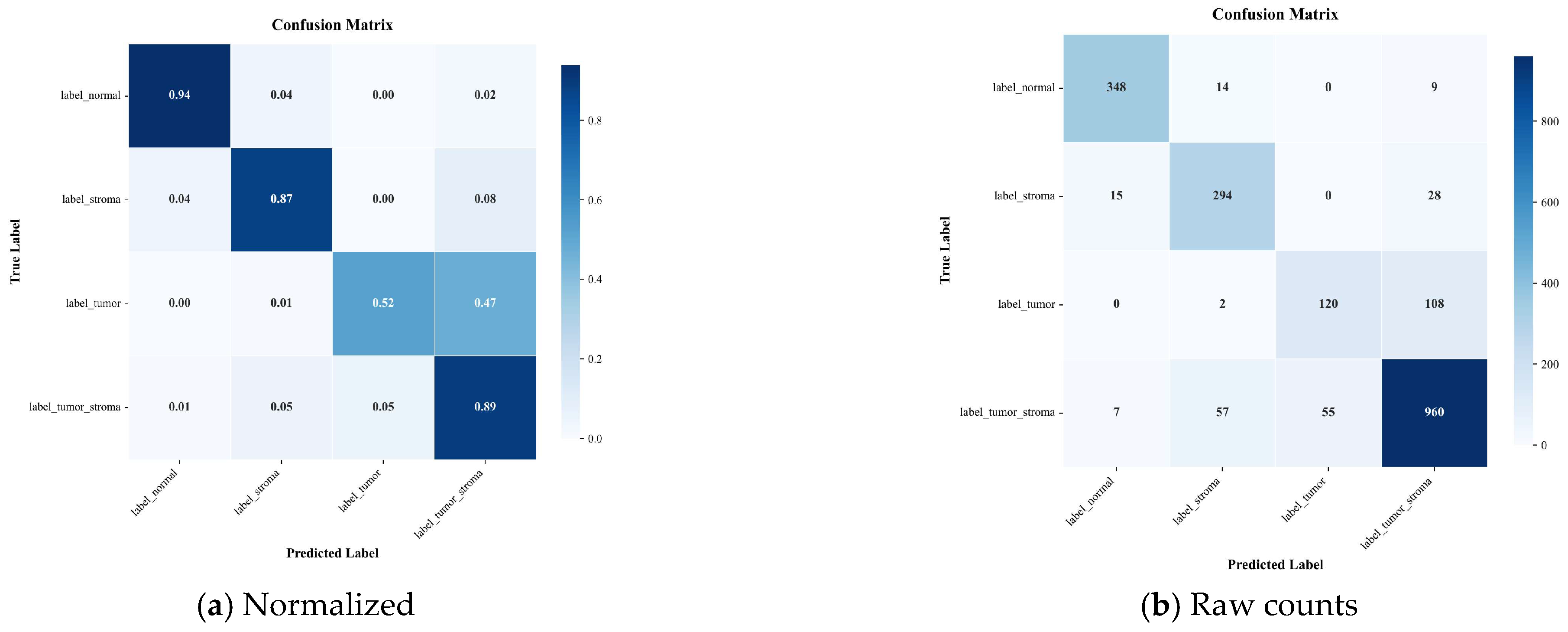
The per-class performance is detailed in Table 10, and the confusion matrix is shown in Figure 11.
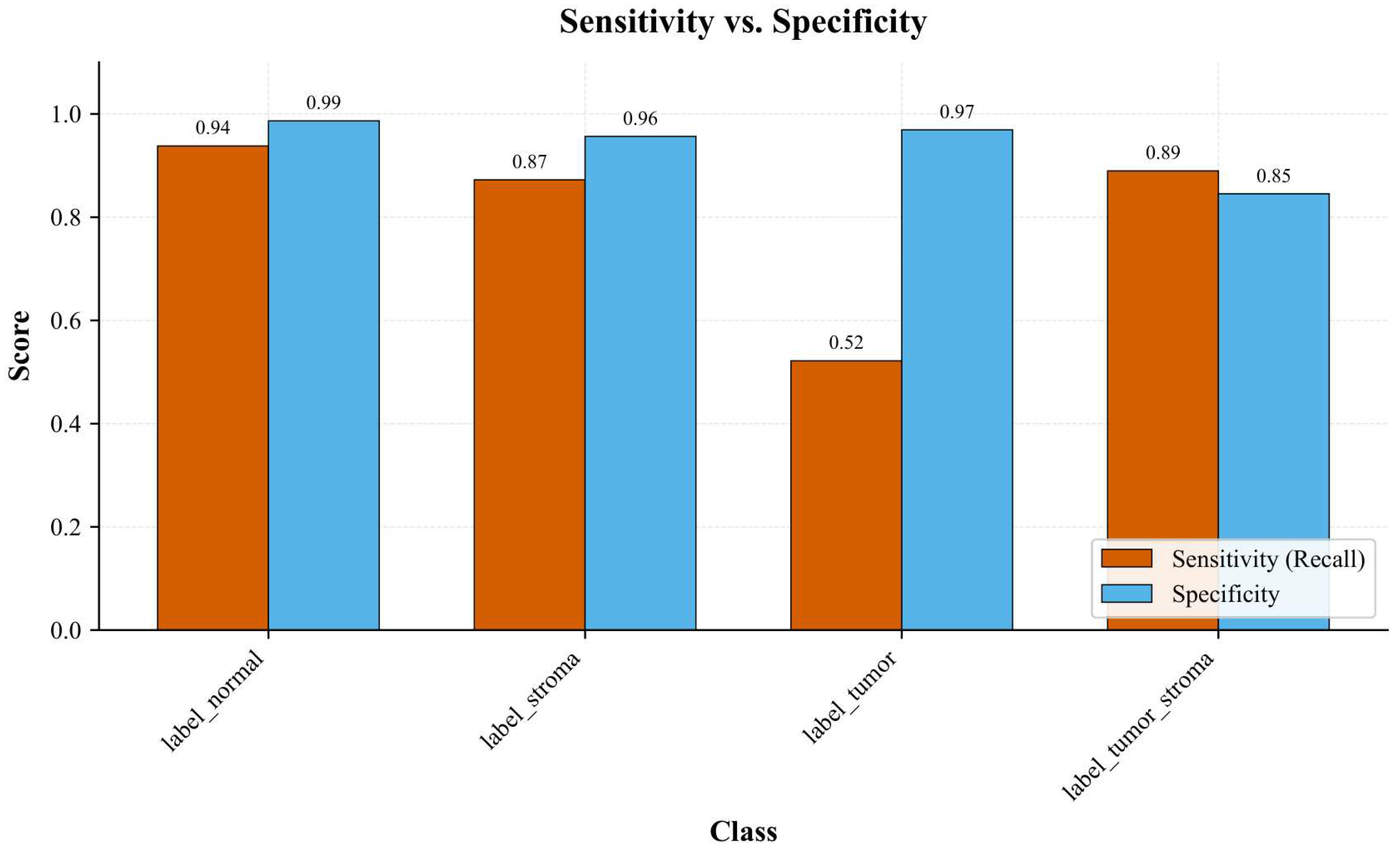
The model demonstrates strong performance in identifying Normal tissue, achieving an F1-score of 0.9393 and a specificity of 0.9866, which may be associated with the distinct morphological characteristics of healthy alveolar tissue. The Tumor-Stroma class also achieves strong performance (F1 = 0.8791), likely influenced by its larger representation within the dataset. The Stroma class exhibits good recall (0.8724) but comparatively lower precision (0.8011), indicating partial overlap with other tissue categories.
The hardest case is the Tumor class with the lowest recall (0.5217) and F1-score (0.5926). This can be explained by two reasons. First: the Tumor is the smallest class with just 1181 samples (11.71%). The class imbalance ratio to the majority class is about 1:4.6, which is quite significant. Second: The Tumor tissue has morphological features that are shared with tumor-associated stroma, thus the boundary between both classes is inherently ambiguous. The specificity was 0.9692, and the model does not misclassify other tissues as tumors frequently. This is clinically safe in terms of false positive rates.
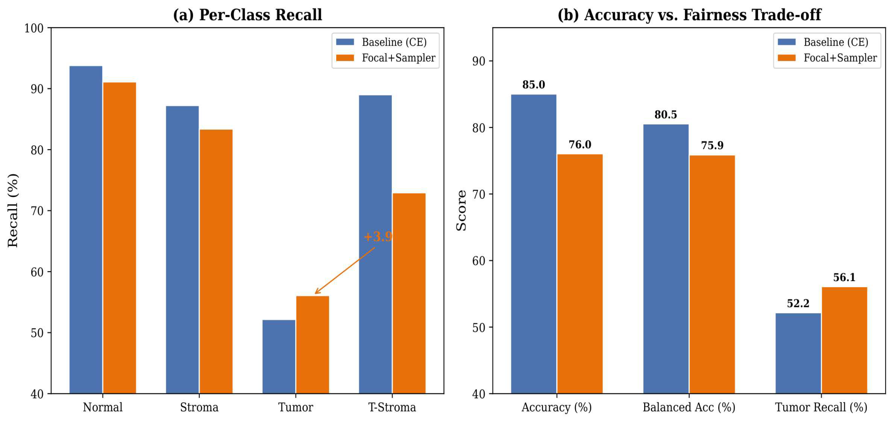
Table 11 summarizes the impact of the proposed class- balancing strategy on per- class performance. To address the low Tumor recall under standard cross-entropy training, we conducted a class-balancing experiment combining Focal Loss ( γ = 2.0 ) [18] with a Weighted Random Sampler that oversamples minority classes using inverse-frequency weights. As shown in Table 8, this strategy improves Tumor recall from 52.17% to 56.09% (+3.92 pp) while the balanced accuracy decreases from 80.55% to 75.88%. The overall accuracy decreases from 85.03% to 76.05%, reflecting the well-known accuracy–fairness trade-off: rebalancing shifts the decision boundary to favor minority classes at the expense of majority-class performance (Tumor-Stroma recall drops from 89.01% to 72.94%). The macro F1-score is 0.7257 versus 0.8077 for the baseline. These results demonstrate that explicit class-balancing can meaningfully improve Tumor detection, though at the cost of overall accuracy. In practice, the relative cost of missing tumors versus false alarms determines the choice of operating point, but a clinician-in-the-loop system that utilizes the top-3 accuracy of 99.60% can further diminish this limitation.
Figure 12 provides a detailed visualization of the class-balancing effect, showing per-class recall changes and the accuracy–fairness trade-off.
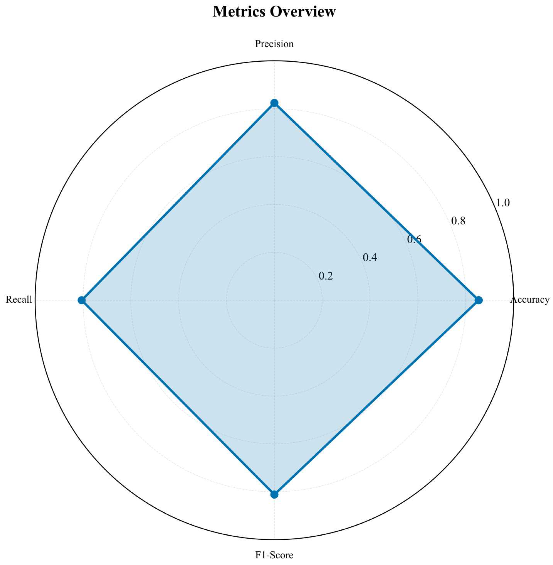
The per-class metrics radar chart is shown in Figure 13 and the sensitivity–specificity comparison is presented in Figure 14.
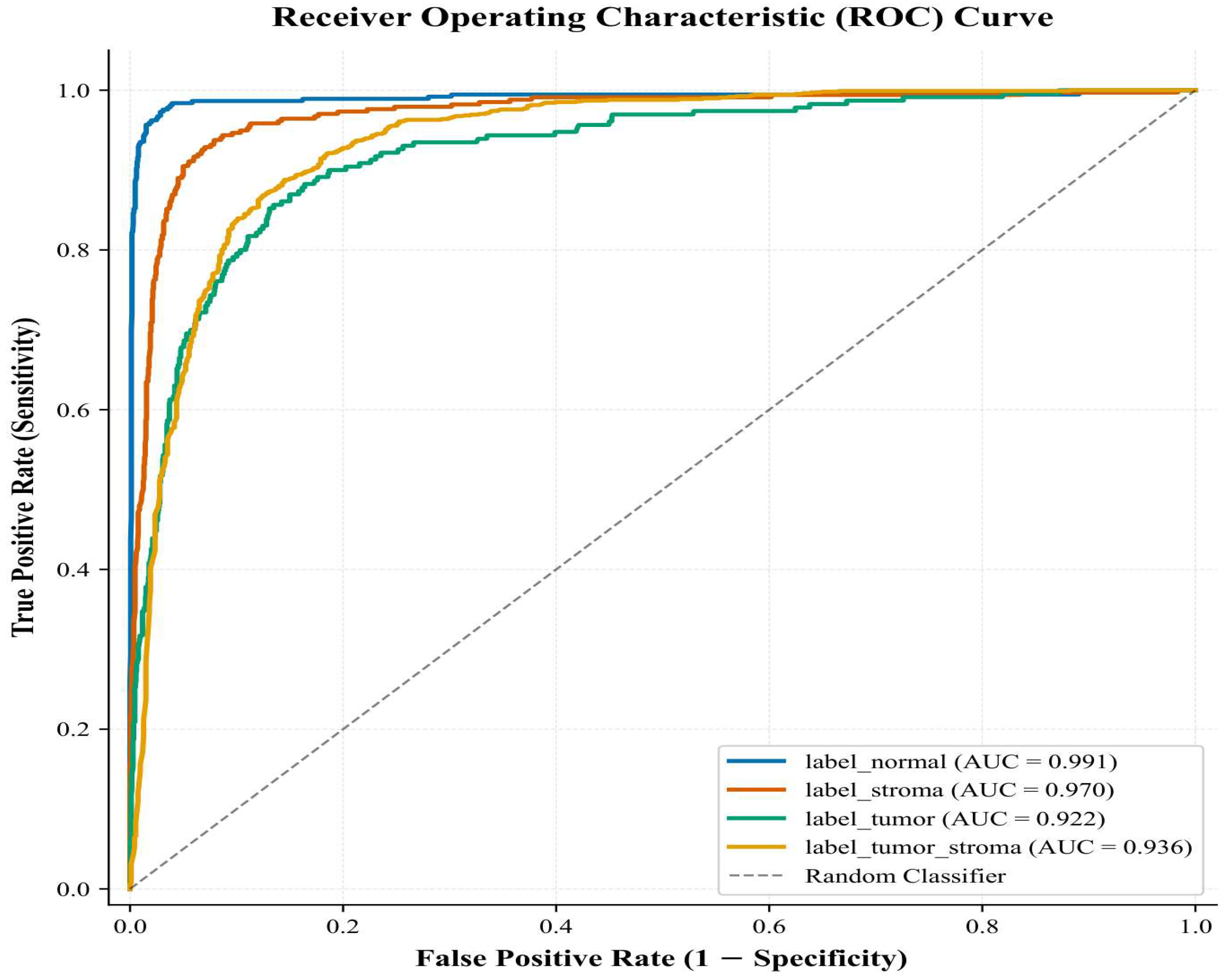
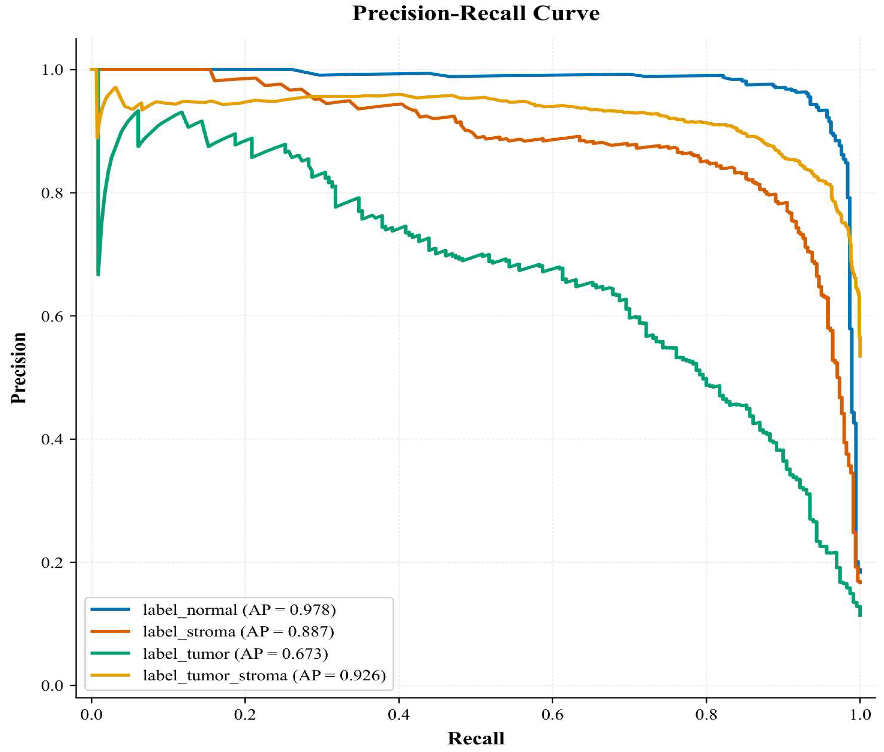
The ROC curves for each class are shown in Figure 15, and the precision–recall curves are presented in Figure 16.

5.7. Medical Accuracy Metrics

Following the medical accuracy formulation in [29], the patch-level accuracy is η p = 85.03 % . Since the current evaluation operates at the patch level without WSI-level majority voting, η w = η p and η tot = η p × η w / 100 = 72.30 % . In a deployed clinical system with majority voting from the same WSI across patches, η w would be expected to be greater than η p , as shown in [11] where η w (99.47%) is greater than η p (99.40%), to given η tot = 98.87 % . WSI-level aggregation is important work to be done in the future.
The balanced accuracy of 80.55% is computed by taking the average of the per-class recall values, which is more representative of the performance across imbalanced classes. The ECE value of 0.0378 means that the model’s predicted probabilities are similar to the actual outcome frequencies, which is essential for trustworthy clinical decision support.
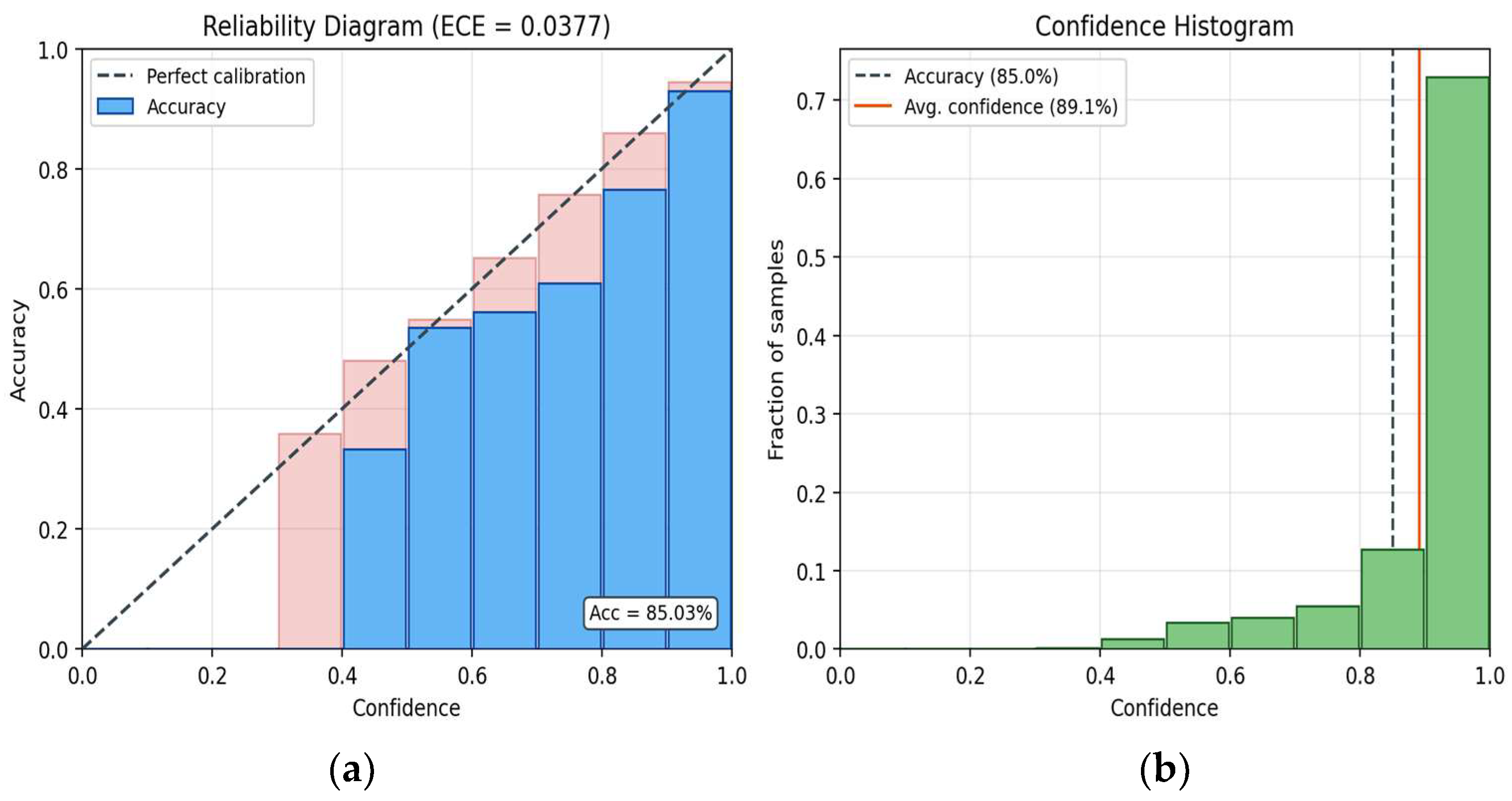
Reliability analysis and per-class calibration. To examine calibration in more detail, Figure 17 presents the reliability diagram and confidence histogram computed on the validation set with ten equal-width confidence bins. The model is calibrated intrinsically: we apply label smoothing (ε = 0.05, Equation (15)) during training and deliberately use no post hoc temperature scaling or Platt scaling, so the reported probabilities are those produced directly by the softmax. The reliability curve tracks the diagonal closely and yields an overall Expected Calibration Error (ECE) of 0.0377, with a small, characteristic over-confidence (mean confidence 89.1% versus 85.0% accuracy). Calibration is, however, not uniform across tissue classes. The per-class ECE is 0.047 for Normal, 0.021 for Stroma, 0.030 for Tumor-Stroma, and 0.297 for the minority Tumor class. The Tumor class is therefore markedly less well calibrated than the others, mirroring its low recall (52.17%) and small sample size (11.71%); the network is over-confident precisely where it is least accurate. This finding reinforces our class-imbalance analysis (Section 5.6) and is clinically important, because reliable confidence estimates for the malignant class are the most consequential. It motivates class-conditional calibration (e.g., per-class temperature scaling) as future work.

5.8. Architectural Comparison

Table 12 contrasts the key design choices between LGFFEM and our framework.
The two methods are based on a similar ConvNeXt V2 backbone and fuse information from multiple scales, but have very different designs and scopes. LGFFEM focuses exclusively on retrieval: it extracts compact embeddings via GeM pooling, trained with ArcFace loss to maximize inter-class separation in embedding space. The BiFPN-inspired neck uses Local and Global Feature Aggregators with channel attention (squeeze-and-excitation style) and learnable fast-normalized fusion weights. Our framework is a dual-purpose system that simultaneously performs classification and retrieval. We augment the backbone with CBAM (channel + spatial attention), use an Adaptive Weighted Fusion neck with softmax-normalized learnable weights, and produce a high-dimensional 18,496-D Hybrid Representation that concatenates global, spatial, and attention-weighted features. This richer descriptor enables both calibrated classification (ECE = 0.0378 ) and content-based retrieval (MAP = 0.8323 ).

5.9. Retrieval Accuracy Comparison

Table 13 compares retrieval accuracy using the medical accuracy metrics η p , η w , and η tot . Because LGFFEM used three progressive training strategies (A: ImageNet-1K only; B: +PanNuke; C: +Kimia Patch24C), we include all three to illustrate the effect of domain-specific pre-training.
From this comparison several conclusions can be drawn:
1.
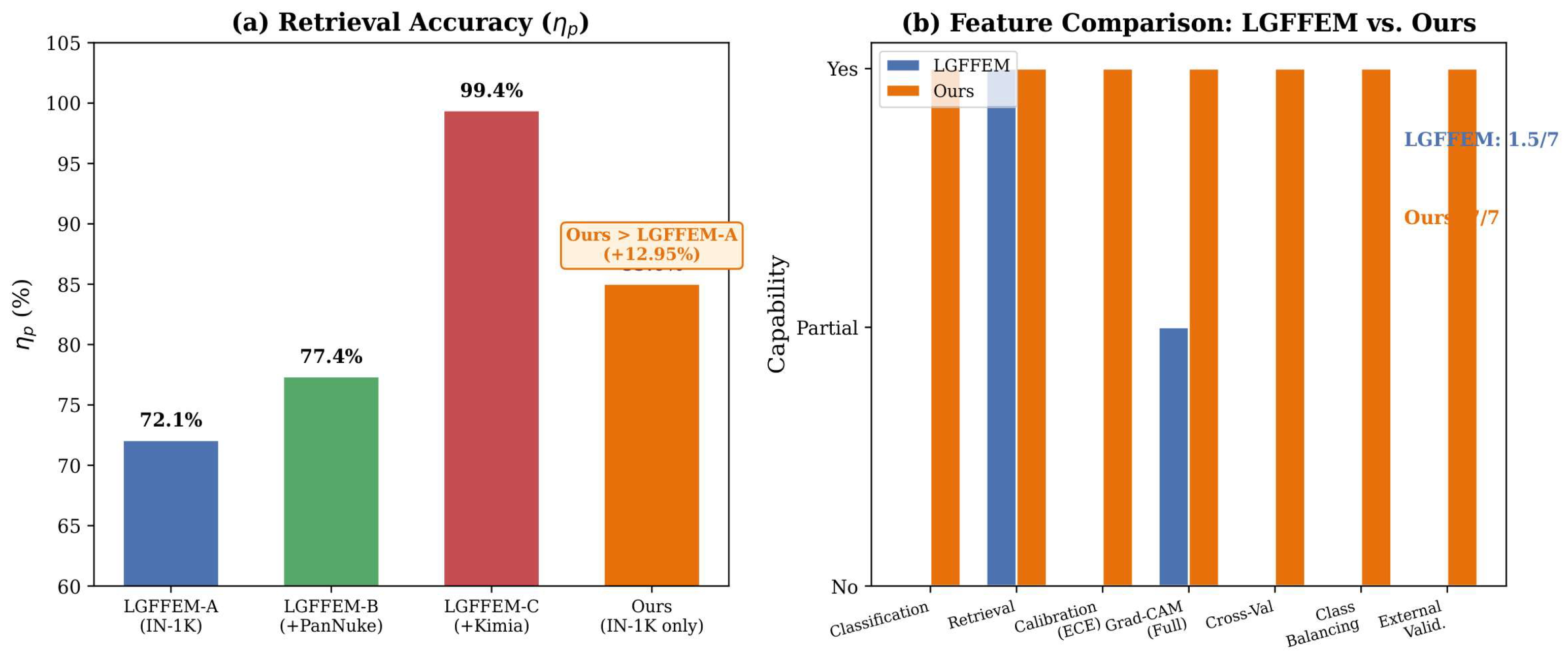
Difficulty of the Dataset: LGFFEM-A, trained on ImageNet-1K without domain data, and performs at η p = 72.08 % on Kimia Patch24C, which is lower than our 85.03% on WSSS4LUAD. This shows that our model is not only able to compete with the other baselines despite the lack of domain-specific pre-training on the target set, it also uses only ImageNet initialization.
2.
The importance of domain-specific training: LGFFEM increased from 72.08% (strategy A) to 99.40% (strategy C), the use of the target dataset in the training process is found to be important. This is not a direct comparison with LGFFEM-C because our model was not trained on Kimia Patch24C.
3.
Task granularity: Kimia Patch24C contains 24 visually distinct tissue types from diverse organs, where inter-class boundaries are relatively clear. WSSS4LUAD is a harder classification task per class due to its low class balance (1:4.6 ratio) for 4 morphologically similar lung adenocarcinoma classes.
4.
Multi-task advantage: Our framework yields the advantages of simultaneous classification (85.03%), calibrated probabilities (ECE = 0.0378 ), retrieval (MAP = 0.8323 , MRR = 0.8784 ), and explainability by Grad-CAM, which are critical requirements for the clinical deployment of our framework that are not provided by LGFFEM, and previous works.
Future work will assess our framework on Kimia Patch24C to allow for a direct comparison between the different test setup and investigate adding domain-specific pre-training (e.g., PanNuke) to help the accuracy gap.
The accuracy of retrieval and the system capabilities are visually compared in Figure 18 between LGFFEM and our framework.

5.10. Retrieval Performance

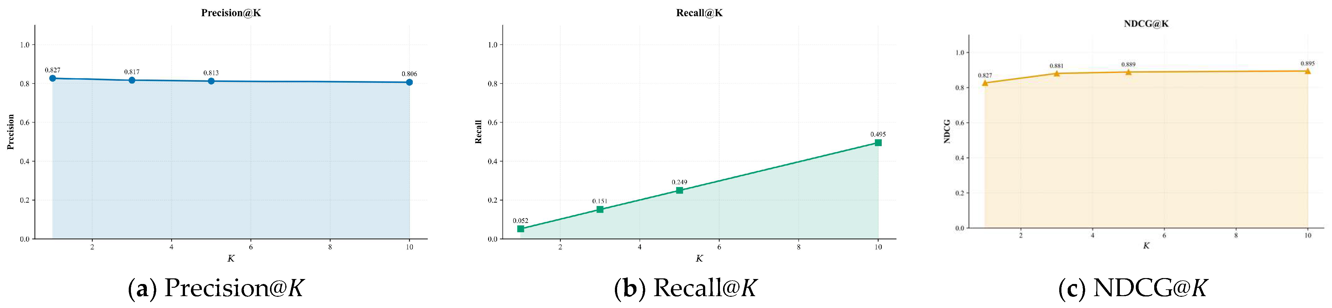
Table 14 summarizes the content-based image retrieval performance. The retrieval metrics at different values of K are also visualized in Figure 19.
The retrieval system has a Precision@1 value of 0.8270, with the 82.70% of queries having the most similar retrieved image in the correct tissue class. All query images rank well with an average of 0.8323. The MRR value is 0.8784, indicating that the first image retrieved is usually the highest one in the ranked list. The NDCG values, NDCG@K, rise monotonically from 0.8270 to 0.8948 with the increase of K, which shows that the retrieval ranking is relevant to the images. The relatively low Recall@ K values at small K are expected, given the large number of relevant images in the database for the majority classes.
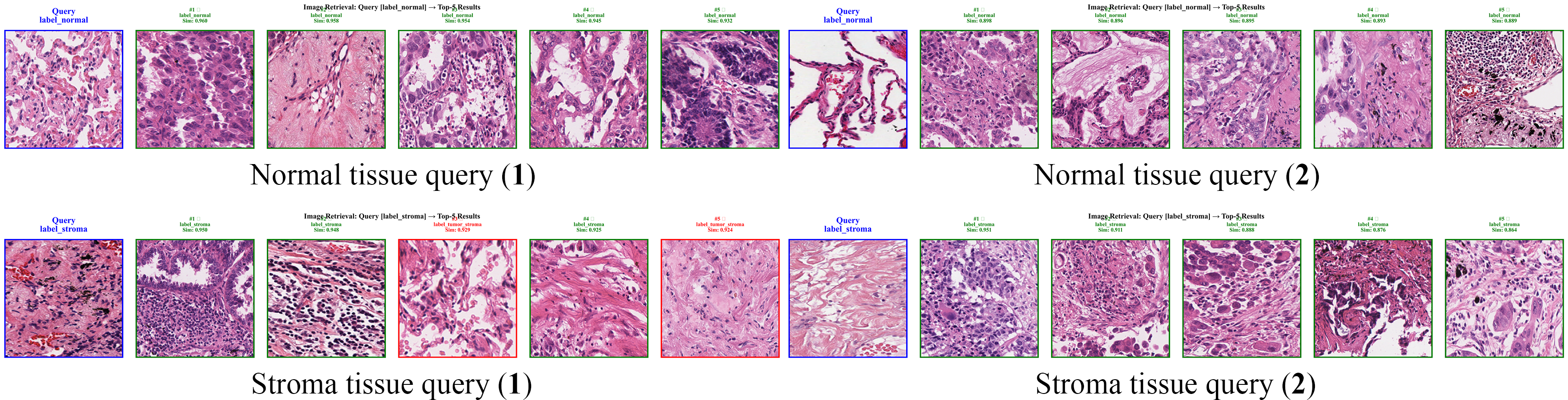
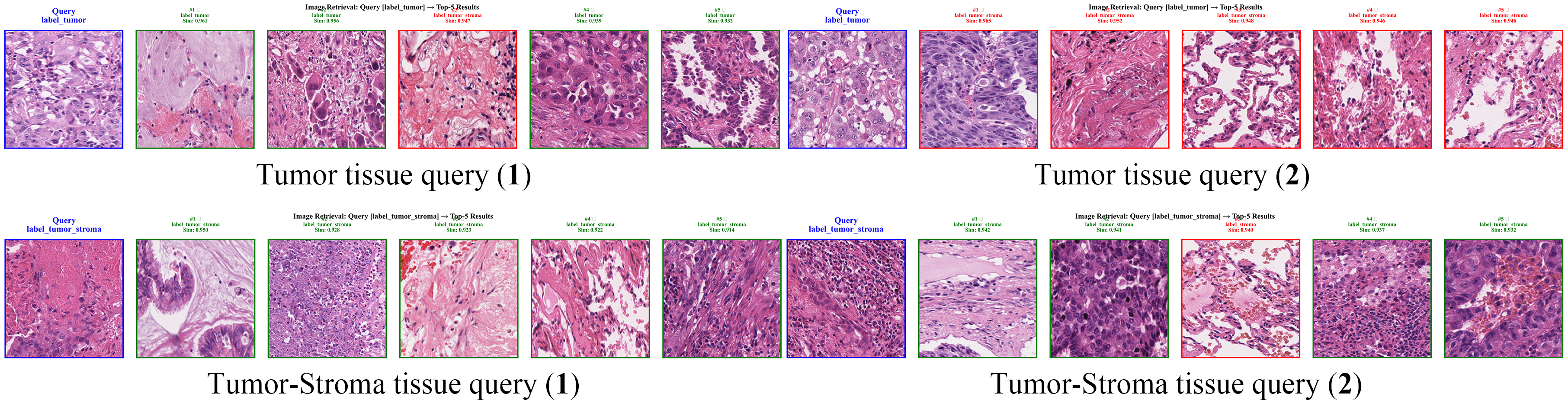
Figure 20 and Figure 21 show qualitative retrieval examples for each tissue class, where the query image is shown alongside its top-5 retrieved results.

6. Discussion

This section provides a comprehensive interpretation of the proposed framework’s performance. The analysis focuses on explainability, comparative behavior with existing CBHIR approaches, and the overall balance between retrieval accuracy, classification capability, and computational efficiency. Furthermore, the discussion highlights the strengths, limitations, and potential clinical relevance of the proposed system in real-world histopathological image retrieval applications.

6.1. Relation to Existing CBHIR Methods

Several content-based histopathological image retrieval (CBHIR) methods have been proposed in recent years. Babaie et al. [29] demonstrated the effectiveness of DenseNet-121 features for patch retrieval on the Kimia Patch24C benchmark, achieving η p = 95.92 % . Yang et al. [12] improved upon this with a multi-attention and multi-scale (MA+MS) approach, reaching η p = 97.89 % on the same benchmark. Most recently, Núñez et al. [11] proposed the Local–Global Feature Fusion Embedding Model (LGFFEM), a lightweight 14.5M-parameter model built on ConvNeXt V2 with a BiFPN-inspired neck and GeM pooling head, trained with Sub-center ArcFace loss [31], achieving state-of-the-art η p = 99.40 % on Kimia Patch24C. Since LGFFEM shares our ConvNeXt V2 backbone and multi-scale fusion philosophy, we provide a detailed architectural and performance comparison below.

6.2. Explainability Analysis with Grad-CAM

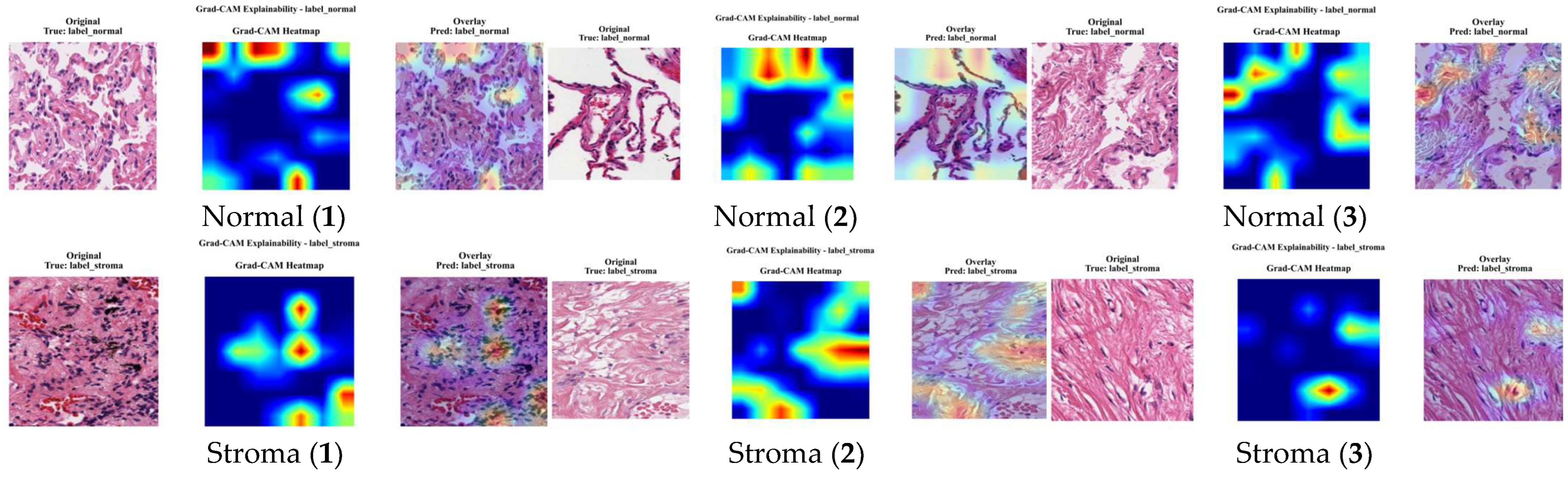
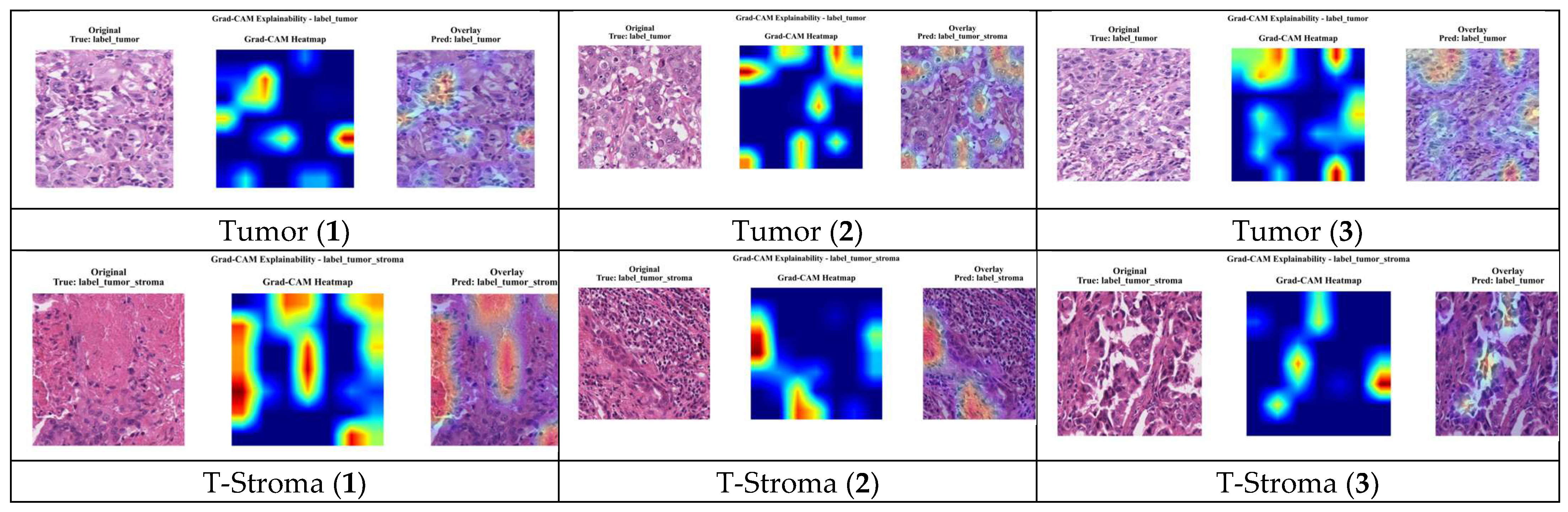
In line with the growing emphasis on explainable artificial intelligence for transparent and trustworthy cancer-detection systems [32], we provide interpretable insights into the model’s decision-making process, we apply Grad-CAM to the final backbone stage (backbone.stages. 3) for representative images from each class, as shown in Figure 22 and Figure 23.
In the case of Normal tissue samples, the Grad-CAM visualizations demonstrate broad focus over the alveolar spaces, suggesting that the model’s predictions are based on the overall structure of healthy tissue and not on specific cellular patterns. The stroma samples show a focus on the fibers of the dense connective tissue, which are especially dense in the areas of collagen bundles.
The activation maps show regions of unusual cells with nuclei that are not normally shaped for Tumor samples, indicating that the model has become proficient in recognizing the signatures of abnormal cells. As a result of the mixed nature of this tissue class, activations in Tumor-Stroma samples are distributed between the epithelial tumor component and the surrounding reactive stroma, as shown by the dual attention patterns. These visualizations validate the model to have learned pathologically meaningful features and give a tool for clinicians to check and believe the model’s prediction.
Validity and scope of the explainability analysis. We emphasize that the Grad-CAM maps in this study were assessed qualitatively by the authors against the expected histological appearance of each class—diffuse activation over alveolar spaces for Normal, collagen-fiber emphasis for Stroma, abnormal-nuclei clusters for Tumor, and dual epithelial/stromal attention for Tumor-Stroma—rather than through a formal reader study. The maps were not yet reviewed by board-certified pathologists, and we did not quantitatively compare the highlighted regions against pixel-level tumor annotations, because the patch-level WSSS4LUAD labels we use do not provide dense region masks. The present evidence that the model attends to diagnostically plausible structures should therefore be read as supportive but not confirmatory. A rigorous validation—measuring the overlap between Grad-CAM saliency and expert or weakly-supervised tumor annotations, and a pathologist-in-the-loop agreement study—is an important direction we identify for future work (Section 7), and would turn explainability from a visual aid into a quantitatively validated component.

6.3. Multi-Criteria Summary

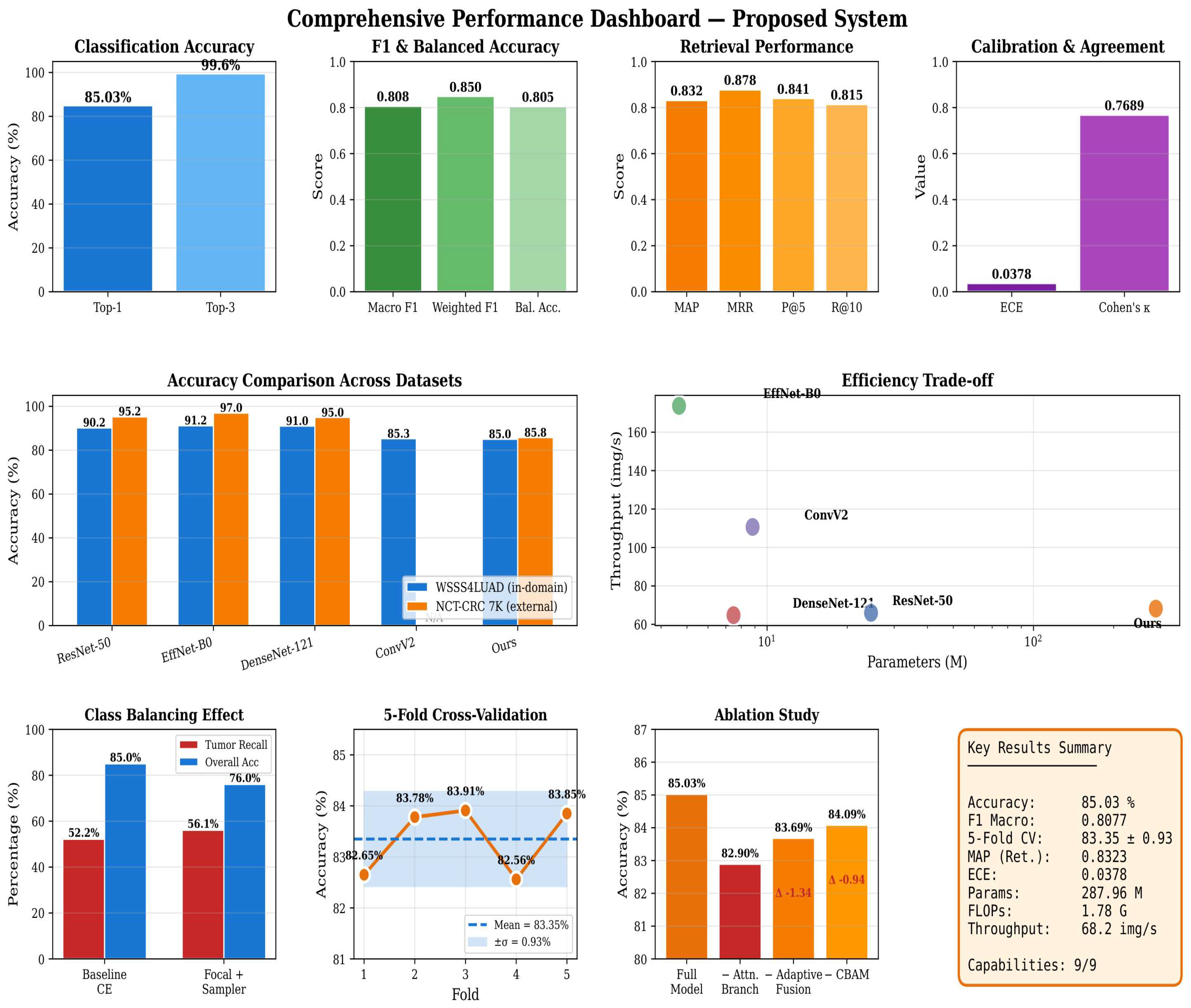
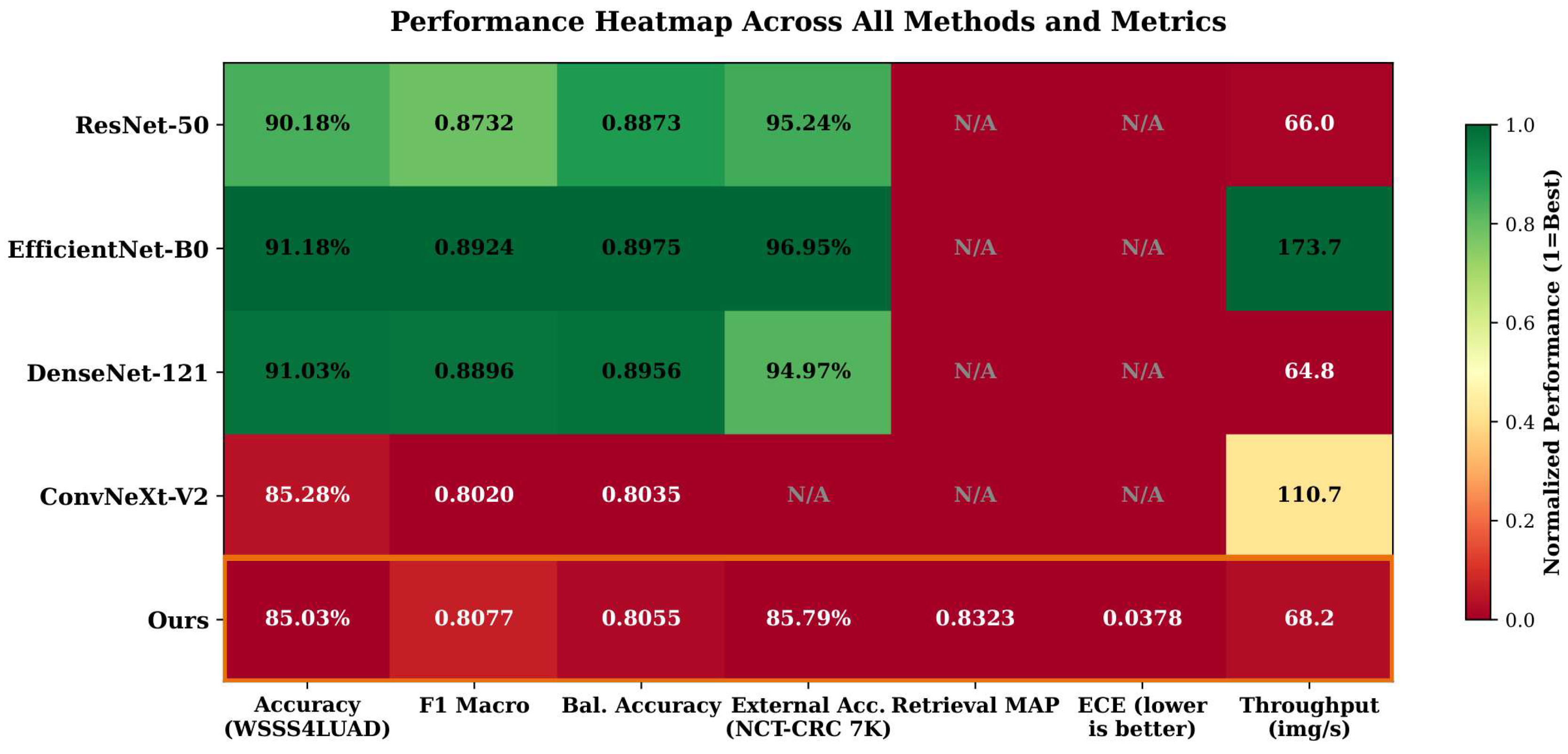
All important quantitative results are consolidated on one dashboard for the proposed system, as shown in Figure 24, to give a complete overview of the strengths of the proposed system, which include classification, F1 scores, retrieval, calibration, external validation, efficiency trade-off, class balancing, k-fold stability, and ablation. In Figure 25, we complement this with a color-coded comparison of all methods and metrics so that it can be easily seen where our model is missing from the baselines.
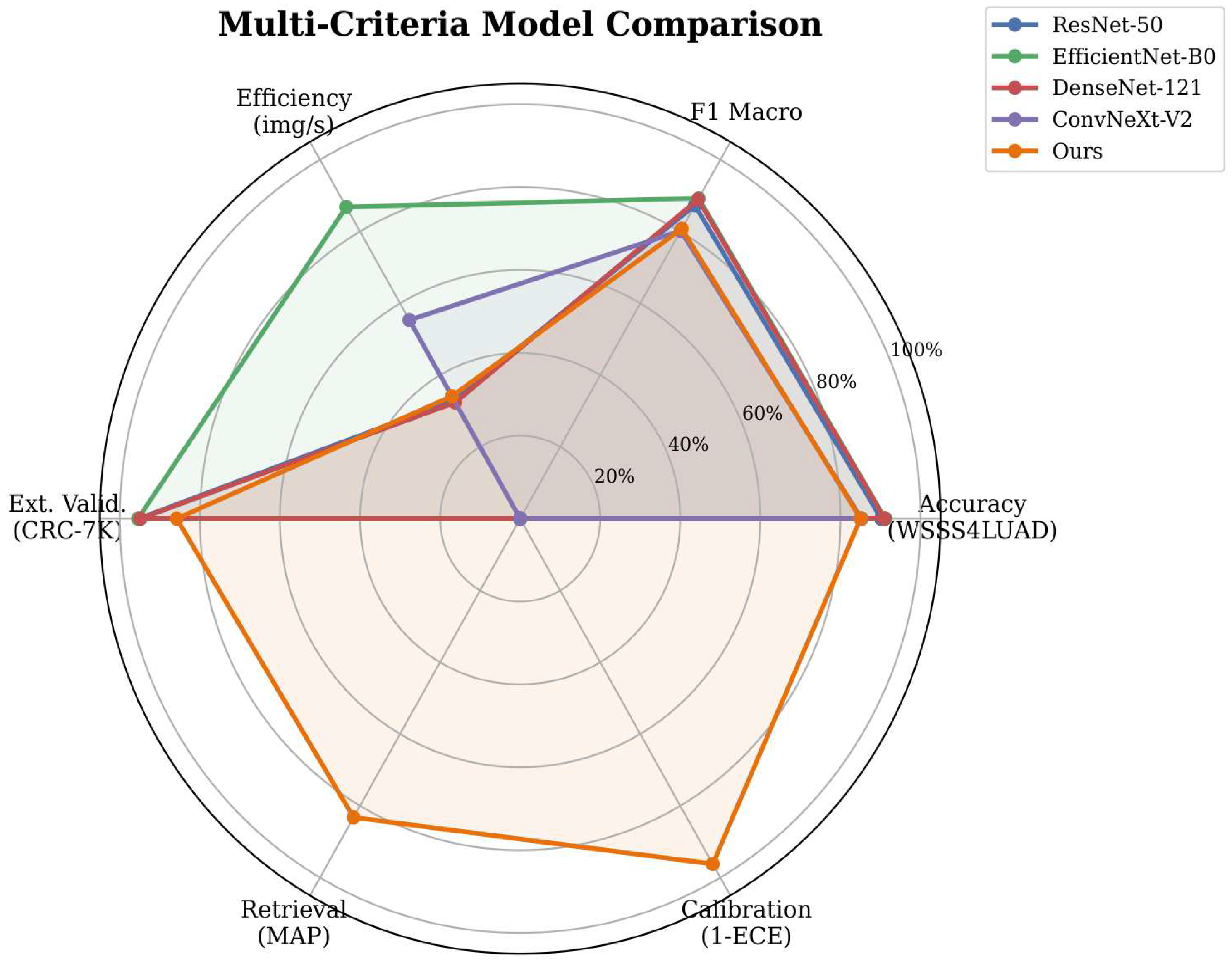
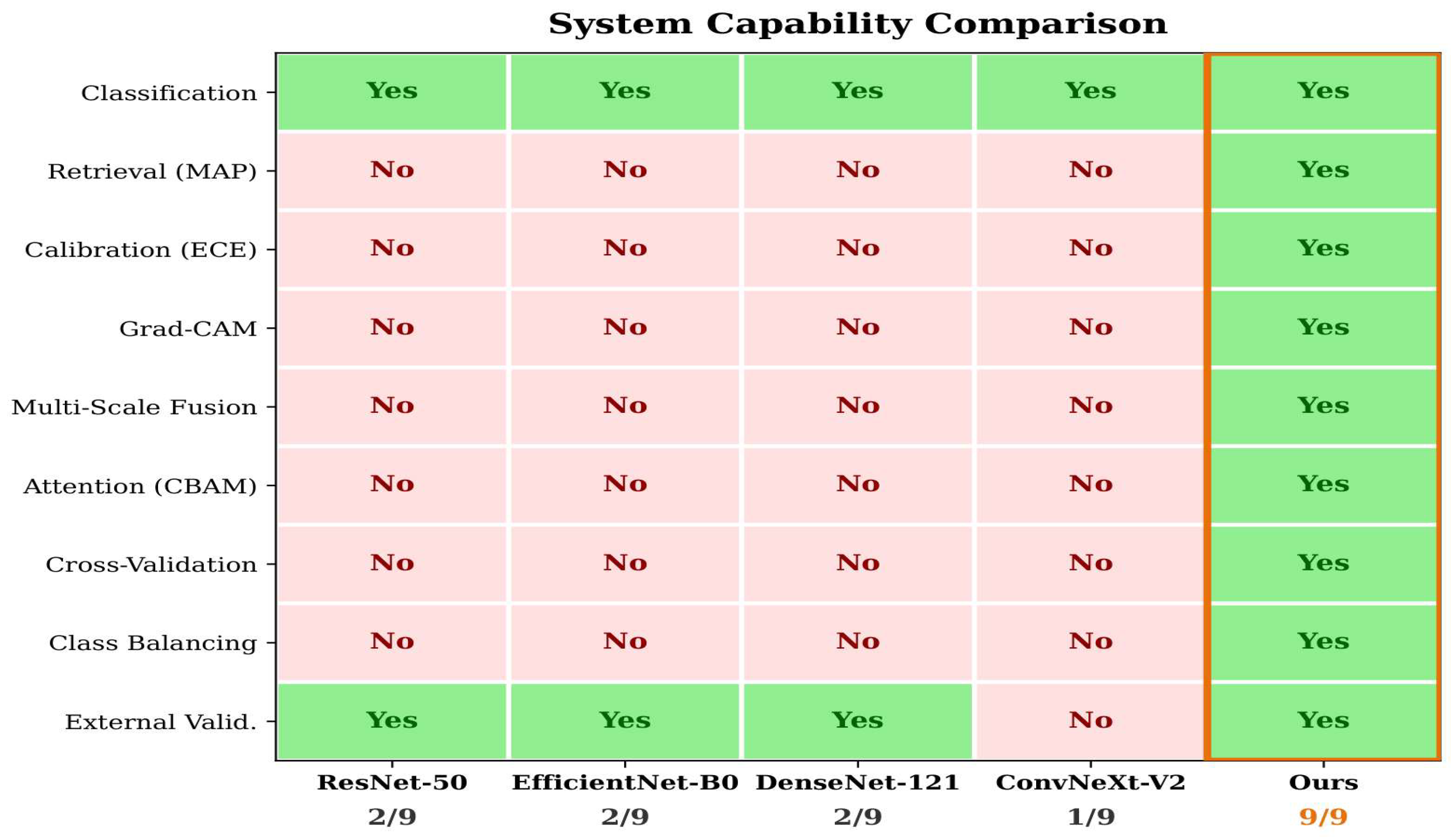
Figure 26 and Figure 27 take a focused view: a multi-criteria radar chart comparing all evaluated models across six evaluation dimensions, and a capability matrix summarizing which features each model supports.
Our proposed framework is the only architecture with all nine of the evaluated capabilities namely classification, retrieval, calibration, Grad-CAM explainability, multi-scale fusion, attention mechanism, cross validation, class balancing and external validation, while the baseline architectures only offer 5–6% classification accuracy on WSSS4LUAD. The mix of these capabilities is ideal for clinical deployment, where the confidence in and the interpretability of predictions is as critical as the accuracy of the predictions themselves.

7. Conclusions

We now sum up and peer into the future. We developed and applied a single framework for the classification and retrieval of histopathological images, which we applied to the lung adenocarcinoma dataset WSSS4LUAD. The architecture incorporates a ConvNeXt V2 backbone with CBAM attention, an Adaptive Weighted Fusion Neck with learnable softmax-normalized weights and a Hybrid Representation Head that projects a 18,496-dim descriptor from the global, spatial and attention-weighted representations.
The following results are reported:
  • An overall classification accuracy of 85.03% with a 5-fold cross-validation mean of 83.35 ± 0.93%, confirming statistical robustness on a four-class LUAD tissue classification task.
  • A systematic ablation study confirming the contribution of each proposed module: the Attention Branch (Δ = −2.13%), Adaptive Fusion (Δ = −1.34%), and CBAM (Δ = −0.94%) all contribute positively.
  • Competitive inference throughput (68.2 img/s, 1.78 GFLOPs) despite the large parameter count (287.96 M), with latency comparable to ResNet-50.
  • Strong retrieval performance with MAP of 0.8323 and MRR of 0.8784, enabling effective content-based image search.
  • Well-calibrated predictions with ECE of 0.0378, suitable for clinical decision support.
  • A class-balancing experiment showing that Focal Loss with Weighted Random Sampling improves Tumor recall from 52.17% to 56.09%, illustrating the accuracy–fairness trade-off inherent in imbalanced histopathology datasets.
  • Cross-organ generalization validated on NCT-CRC-HE-100K → CRC-VAL-HE-7K (9 colorectal tissue classes), where our model achieves 85.79% accuracy using only 10.8 K training images (vs. 100 K for baselines), confirming transferability of the learned representations across organs.
Combined, these results highlight a trade-off: the model’s accuracy on raw WSSS4LUAD is 5–6% lower than that of lightweight classifiers (EfficientNet-B0: 91.18%, DenseNet-121: 91.03%), but retrieval (MAP = 0.8323), calibration (ECE = 0.0378 Grad-CAM explainability and capabilities are descriptive features that none of the baselines can offer.
Although these results were found, several limitations were encountered. The first four are summarized below, followed by additional considerations raised during peer review:
  • Large model size: Using 287.96 M parameters, the answer is almost 20 times higher than LGFFEM (14.5 M) and 60 times higher than EfficientNet-B0, which can be important for deployment on resource-constrained clinical devices.
  • Class imbalance was partially mitigated: The combination of Focal Loss with Weighted Random Sampling slightly improved the Tumor recall rate from 52.17% to 56.09%, while decreasing the overall accuracy (85.03% → 76.05%). This gap can be further closed by more advanced strategies (e.g., curriculum learning, two-stage training).
  • Limited external validation: Results with NCT-CRC-HE-100K → CRC-VAL-HE-7K (85.79%) indicate cross-organ generalization, but our model was trained on a subsample of 10.8 K, because of the computational needs.
  • Patch-level evaluation: Evaluations were conducted only at the patch level, whereas majority voting at the WSI level would be required for clinical deployment.
Beyond these four, we acknowledge the following: (5) Single-dataset development—the architecture was developed and tuned on one in-domain benchmark (WSSS4LUAD); broader validation across multiple LUAD cohorts is needed. (6) Patch-level rather than slide-level splitting—because the public release does not expose slide identifiers for every patch; our split is at the patch level, which can allow same-slide patches to fall in both training and validation and may optimistically bias results; a strict patient/slide-level split is required for a fully leakage-free estimate. (7) Staining and scanner variability—H&E color and scanner characteristics differ across laboratories, and although color augmentation mitigates this, robustness to domain shift across institutions has not been quantified. (8) High descriptor dimensionality—the 18,496-D descriptor, while well-justified at this scale, may require compression (PCA, product quantization, or hashing) before deployment to whole-slide-sized archives. (9) Class-conditional reliability—calibration is good overall but degrades for the minority Tumor class (per-class ECE 0.297), so confidence estimates for malignant predictions should be used cautiously until class-conditional calibration is applied. (10) Sensitivity to noisy labels and rare patterns—the effect of label noise and the behavior on rare or atypical tissue patterns were not systematically studied. (11) Explainability not yet formally validated—Grad-CAM maps were assessed qualitatively and have not been reviewed by pathologists or compared against region annotations.
Building on these findings, we plan four follow-ups: (1) reducing model complexity through knowledge distillation or a leaner backbone; (2) advanced class-balancing (curriculum learning, two-stage fine-tuning) to raise Tumor recall without sacrificing overall accuracy; (3) retraining on the full NCT-CRC-HE-100K with GPU acceleration and validating on additional benchmarks, such as Kimia Patch24C; and (4) extending evaluation to WSI-level inference with spatial aggregation.
We further plan to (5) raise Tumor sensitivity through ensemble strategies (e.g., bagging of complementary backbones or a two-expert tumor/non-tumor cascade), which trade a modest increase in inference cost for improved minority-class recall; (6) apply class-conditional calibration so that confidence estimates remain reliable for the malignant class; (7) enforce a strict slide- or patient-level split and quantify robustness to staining and scanner domain shift; and (8) carry out a pathologist-in-the-loop study that validates the Grad-CAM saliency against expert annotations. Situated in a real computational-pathology workflow, the proposed framework is intended to operate as an integrated decision-support component: given a query patch or region, it provides a calibrated tissue-classification probability, retrieves visually similar, previously confirmed cases from an indexed archive for case-based comparison and second-reading, and overlays a Grad-CAM saliency map that lets the pathologist verify the basis of each prediction. Such a system could support routine LUAD tissue classification, case-based diagnostic review, rare-pattern look-up, quality control, and trainee education, while the explicit reporting of calibration and per-class behavior helps the user judge when the model’s output should be trusted and when a confirmatory human read is warranted.

Author Contributions

Conceptualization, N.S.A. and F.M.; methodology, N.S.A. and F.M.; software, N.S.A.; validation, N.S.A., F.M. and J.K.; formal analysis, N.S.A.; investigation, N.S.A.; resources, N.S.A.; data curation, N.S.A.; writing—original draft preparation, N.S.A.; writing—review and editing, F.M., J.K. and N.S.A.; visualization, N.S.A.; supervision, F.M. and J.K.; project administration, F.M. and J.K.; funding acquisition, N.S.A. All authors have read and agreed to the published version of the manuscript.

Funding

This research received no external funding.

Data Availability Statement

The WSSS4LUAD dataset is publicly available. The source code, trained model weights, and evaluation scripts for reproducing the results presented in this paper will be made publicly available upon acceptance at https://github.com/shihabahmednoor-beep/hybrid-cbhir-luad (accessed on 12 May 2026).

Conflicts of Interest

The authors declare no conflicts of interest.

References

  1. Sung, H.; Ferlay, J.; Siegel, R.L.; Laversanne, M.; Soerjomataram, I.; Jemal, A.; Bray, F. Global cancer statistics 2020: GLOBOCAN estimates of incidence and mortality worldwide for 36 cancers in 185 countries. CA Cancer J. Clin. 2021, 71, 209–249. [Google Scholar] [CrossRef] [Scilit] [PubMed]
  2. Solar, M.; Aguirre, P. Deep learning techniques to process 3D chest CT. J. Univers. Comput. Sci. 2024, 30, 758. [Google Scholar] [CrossRef] [Scilit]
  3. Rahaman, M.M.; Li, C.; Wu, X.; Yao, Y.; Hu, Z.; Jiang, T.; Li, X.; Qi, S. A survey for cervical cytopathology image analysis using deep learning. IEEE Access 2020, 8, 61687–61710. [Google Scholar] [CrossRef] [Scilit]
  4. Hegde, N.; Hipp, J.D.; Liu, Y.; Emmert-Buck, M.; Reif, E.; Smilkov, D.; Terry, M.; Cai, C.J.; Amin, M.B.; Mermel, C.H.; et al. Similar image search for histopathology: SMILY. npj Digit. Med. 2019, 2, 56. [Google Scholar] [CrossRef] [Scilit] [PubMed]
  5. Hashimoto, N.; Takagi, Y.; Masuda, H.; Miyoshi, H.; Kohno, K.; Nagaishi, M.; Sato, K.; Takeuchi, M.; Furuta, T.; Kawamoto, K.; et al. Case-based similar image retrieval for weakly annotated large histopathological images of malignant lymphoma using deep metric learning. Med. Image Anal. 2023, 85, 102752. [Google Scholar] [CrossRef] [Scilit] [PubMed]
  6. Kumar, A.; Kim, J.; Cai, W.; Fulham, M.; Feng, D. Content-based medical image retrieval: A survey of applications to multidimensional and multimodality data. J. Digit. Imaging 2013, 26, 1025–1039. [Google Scholar] [CrossRef] [Scilit] [PubMed]
  7. Abdelsamea, M.M.; Zidan, U.; Senousy, Z.; Gaber, M.M.; Rakha, E.; Ilyas, M. A survey on artificial intelligence in histopathology image analysis. Wiley Interdiscip. Rev. Data Min. Knowl. Discov. 2022, 12, e1474. [Google Scholar] [CrossRef] [Scilit]
  8. Sikaroudi, M.; Hosseini, M.; Gonzalez, R.; Rahnamayan, S.; Tizhoosh, H.R. Generalization of vision pre-trained models for histopathology. Sci. Rep. 2023, 13, 6065. [Google Scholar] [CrossRef] [Scilit] [PubMed]
  9. Cao, B.; Araujo, A.; Sim, J. Unifying deep local and global features for image search. In Proceedings of the European Conference on Computer Vision (ECCV), Glasgow, UK, 23–28 August 2020; Springer: Cham, Switzerland, 2020; pp. 726–743. [Google Scholar] [CrossRef] [Scilit]
  10. Iqbal, S.; Qureshi, A.N.; Alhussein, M.; Choudhry, I.A.; Aurangzeb, K.; Khan, T.M. Fusion of textural and visual information for medical image modality retrieval using deep learning-based feature engineering. IEEE Access 2023, 11, 93238–93253. [Google Scholar] [CrossRef] [Scilit]
  11. Nuñez-Fernández, C.; Farias, H.; Solar, M. Content-based histopathological image retrieval. Sensors 2025, 25, 1350. [Google Scholar] [CrossRef] [Scilit] [PubMed]
  12. Yang, P.; Zhai, Y.; Li, L.; Lv, H.; Wang, J.; Zhu, C.; Jiang, R. A deep metric learning approach for histopathological image retrieval. Methods 2020, 179, 14–25. [Google Scholar] [CrossRef] [Scilit] [PubMed]
  13. Tabatabaei, Z.; Colomer, A.; Moll, J.O.; Naranjo, V. Toward more transparent and accurate cancer diagnosis with an unsupervised CAE approach. IEEE Access 2023, 11, 143387–143401. [Google Scholar] [CrossRef] [Scilit]
  14. Alizadeh, S.M.; Helfroush, M.S.; Muller, H. A novel Siamese deep hashing model for histopathology image retrieval. Expert Syst. Appl. 2023, 225, 120169. [Google Scholar] [CrossRef] [Scilit]
  15. Kather, J.N.; Weis, C.-A.; Bianconi, F.; Melchers, S.M.; Schad, L.R.; Gaiser, T.; Marx, A.; Zöllner, F.G. Multi-class texture analysis in colorectal cancer histology. Sci. Rep. 2016, 6, 27988. [Google Scholar] [CrossRef] [Scilit] [PubMed]
  16. Spanhol, F.A.; Oliveira, L.S.; Petitjean, C.; Heutte, L. A dataset for breast cancer histopathological image classification. IEEE Trans. Biomed. Eng. 2016, 63, 1455–1462. [Google Scholar] [CrossRef] [Scilit] [PubMed]
  17. Tabatabaei, Z.; Colomer, A.; Moll, J.O.; Naranjo, V. Siamese content-based search engine for a more transparent skin and breast cancer diagnosis through historical imaging. arXiv 2024, arXiv:2401.08272. [Google Scholar] [CrossRef] [Scilit]
  18. Lin, T.-Y.; Dollár, P.; Girshick, R.; He, K.; Hariharan, B.; Belongie, S. Feature pyramid networks for object detection. In Proceedings of the IEEE Conference on Computer Vision and Pattern Recognition (CVPR), Honolulu, HI, USA, 21–26 July 2017; IEEE: New York, NY, USA, 2017; pp. 2117–2125. [Google Scholar] [CrossRef] [Scilit]
  19. Tan, M.; Pang, R.; Le, Q.V. EfficientDet: Scalable and efficient object detection. In Proceedings of the IEEE/CVF Conference on Computer Vision and Pattern Recognition (CVPR), Seattle, WA, USA, 13–19 June 2020; IEEE: New York, NY, USA, 2020. [Google Scholar] [CrossRef] [Scilit]
  20. Iqbal, S.; Qureshi, A.N. A heteromorphous deep CNN framework for medical image segmentation using local binary pattern. IEEE Access 2022, 10, 63466–63480. [Google Scholar] [CrossRef] [Scilit]
  21. Hu, J.; Shen, L.; Sun, G. Squeeze-and-excitation networks. In Proceedings of the IEEE Conference on Computer Vision and Pattern Recognition (CVPR), Salt Lake City, UT, USA, 18–22 June 2018. [Google Scholar] [CrossRef] [Scilit]
  22. Woo, S.; Park, J.; Lee, J.-Y.; Kweon, I.S. CBAM: Convolutional block attention module. In Proceedings of the European Conference on Computer Vision (ECCV), Munich, Germany, 8–14 September 2018; IEEE: New York, NY, USA, 2018; pp. 3–19. [Google Scholar] [CrossRef] [Scilit]
  23. Shao, S.; Chen, K.; Karpur, A.; Cui, Q.; Araujo, A.; Cao, B. Global features are all you need for image retrieval and reranking. In Proceedings of the IEEE/CVF International Conference on Computer Vision (ICCV), Paris, France, 2–6 October 2023; IEEE: New York, NY, USA, 2023; pp. 11002–11012. [Google Scholar] [CrossRef] [Scilit]
  24. Woo, S.; Debnath, S.; Hu, R.; Chen, X.; Liu, Z.; Kweon, I.S.; Xie, S. ConvNeXt V2: Co-designing and scaling ConvNets with masked autoencoders. In Proceedings of the IEEE/CVF Conference on Computer Vision and Pattern Recognition (CVPR), Vancouver, BC, Canada, 18–22 June 2023; IEEE: New York, NY, USA, 2023; pp. 16133–16142. [Google Scholar] [CrossRef] [Scilit]
  25. Han, C.; Pan, X.; Yan, L.; Lin, H.; Li, B.; Yao, S.; Lv, S.; Shi, Z.; Mai, J.; Lin, J.; et al. WSSS4LUAD: Grand challenge on weakly-supervised tissue semantic segmentation for lung adenocarcinoma. arXiv 2022, arXiv:2204.06455. [Google Scholar] [CrossRef] [Scilit]
  26. Kather, J.N.; Halama, N.; Marx, A. 100,000 histological images of human colorectal cancer and healthy tissue. Zenodo 2018. [Google Scholar] [CrossRef]
  27. Loshchilov, I.; Hutter, F. Decoupled weight decay regularization. In Proceedings of the International Conference on Learning Representations (ICLR), New Orleans, LA, USA, 6–9 May 2019. [Google Scholar]
  28. Douze, M.; Guzhva, A.; Deng, C.; Johnson, J.; Szilvasy, G.; Mazaré, P.-E.; Lomeli, M.; Hosseini, L.; Jégou, H. The Faiss library. arXiv 2024, arXiv:2401.08281. [Google Scholar] [CrossRef] [Scilit]
  29. Babaie, M.; Kalra, S.; Sriram, A.; Mitcheltree, C.; Zhu, S.; Khatami, A.; Rahnamayan, S.; Tizhoosh, H.R. Classification and retrieval of digital pathology scans: A new dataset. arXiv 2017, arXiv:1705.07522. [Google Scholar] [CrossRef] [Scilit]
  30. Farhoudian, A.; Heidari, A.; Shahhosseini, R. A new era in colorectal cancer: Artificial Intelligence at the forefront. Comput. Biol. Med. 2025, 196, 110926. [Google Scholar] [CrossRef] [Scilit] [PubMed]
  31. Deng, J.; Guo, J.; Liu, T.; Gong, M.; Zafeiriou, S. Sub-center ArcFace: Boosting face recognition by large-scale noisy web faces. In Proceedings of the European Conference on Computer Vision (ECCV), Glasgow, UK, 23–28 August 2020; Springer: Cham, Switzerland, 2020; pp. 741–757. [Google Scholar] [CrossRef] [Scilit]
  32. Toumaj, S.; Heidari, A.; Jafari Navimipour, N. Leveraging explainable artificial intelligence for transparent and trustworthy cancer detection systems. Artif. Intell. Med. 2025, 169, 103243. [Google Scholar] [CrossRef] [Scilit] [PubMed]
Figure 2. End-to-end training and evaluation pipeline of the proposed framework. The six stages cover: (1) input data preparation from WSSS4LUAD, (2) preprocessing with augmentation, (3) the proposed architecture with four components (ConvNeXt V2, CBAM, Adaptive Weighted Fusion, Hybrid Head), (4) four output capabilities (classification, retrieval, calibration, Grad-CAM), (5) multi-criteria evaluation, and (6) external validation on an independent dataset.
Computers 15 00473 g002
Figure 3. Class distribution of the WSSS4LUAD dataset. The dataset exhibits significant class imbalance, with Tumor-Stroma comprising 53.48% of all samples and Tumor being the least represented class at 11.71%.
Computers 15 00473 g003
Figure 4. Overview of the datasets used in our study. (a) WSSS4LUAD class distribution (classes, lung tissue). (b) NCT-CRC-HE-100K class distribution (classes, colon tissue) used for external validation. (c) Proportional size comparison across the three dataset splits. (d) Side-by-side comparison of key dataset properties, highlighting cross-organ generalization (lung colon) and increased class complexity (4 9 classes).
Computers 15 00473 g004
Figure 6. 5-fold stratified cross-validation results. The orange dashed line indicates the mean accuracy (83.35%), and the shaded band represents ± 1 standard deviation (0.93%), demonstrating high consistency across data partitions.
Computers 15 00473 g006
Figure 7. Training dynamics over 150 epochs. (a) Training and validation loss curves showing convergence. (b) Training and validation accuracy curves; best validation accuracy of 86.66% at epoch 98. (c) Cosine annealing learning rate schedule with epoch linear warmup. (d) Generalization gap stabilizing at approximately 7–8% after epoch 100.
Computers 15 00473 g007aComputers 15 00473 g007b
Figure 8. Three evaluation dimensions, grouped comparison. (a) WSSS4LUAD accuracy: baselines lead by 5–6%, (b) F1 macro scores, and (c) external validation on CRC-VAL-HE-7K, where baselines (trained on 100 K) achieve > 94% and our model (trained on 10.8 K) achieves 85.79%. N/A indicates that external validation was not performed for the vanilla ConvNeXt-V2 baseline; therefore, no corresponding accuracy is reported.
Computers 15 00473 g008
Figure 9. Component contribution analysis. Starting from the baseline configuration without attention (82.90%), each module incrementally improves the classification accuracy, with the complete model reaching (85.03%) (+2.13% overall improvement).
Computers 15 00473 g009
Figure 10. Efficiency–accuracy trade-off. The size of the bubbles corresponds to the number of parameters. Our model achieves similar GFLOPs to lightweight baselines while offering retrieval. (MAP = 0.83 ), calibration (ECE = 0.04 ), and Grad-CAM functionality.
Computers 15 00473 g010
Figure 11. Confusion matrices obtained on the WSSS4LUAD validation set. (a) Normalized confusion matrix illustrating the per-class accuracy percentages. (b) Raw confusion matrix presenting the absolute prediction counts.
Computers 15 00473 g011
Figure 12. Class-balancing analysis. (a) Per-class recall: Focal+Sampler improves Tumor recall (+3.92%) at the expense of Tumor-Stroma recall ( 16.07 % ). (b) Overall accuracy drops from 85.03% to 76.05%, illustrating the accuracy–fairness trade-off.
Computers 15 00473 g012
Figure 13. Radar chart of per-class classification metrics. Normal tissue achieves the most balanced and highest performance across all metrics, while Tumor shows the largest gap between precision and recall.
Computers 15 00473 g013
Figure 14. Sensitivity and specificity comparison across tissue classes. All classes achieve specificity above 0.84, with Normal tissue reaching 0.99. The Tumor class shows the largest sensitivity–specificity gap.
Computers 15 00473 g014
Figure 15. Receiver Operating Characteristic (ROC) curves for each tissue class. The area under the curve (AUC) is highest for Normal tissue and lowest for the Tumor.
Computers 15 00473 g015
Figure 16. Precision–Recall curves for each tissue class. The curves reflect the trade-off between precision and recall, with Normal tissue maintaining the highest AP.
Computers 15 00473 g016
Figure 17. Calibration analysis on the WSSS4LUAD validation set. (a) Reliability diagram (10 bins): blue bars are per-bin accuracy, red bars show the gap to the diagonal (perfect calibration); the overall ECE is 0.0377. (b) Confidence histogram: the dashed line marks overall accuracy (85.0%) and the solid line marks mean confidence (89.1%), indicating mild over-confidence. No temperature scaling was applied; calibration is obtained intrinsically through label smoothing.
Computers 15 00473 g017
Figure 18. LGFFEM vs. Ours. (a) Retrieval accuracy: the proposed model achieves (85.03%) accuracy, exceeding the (72.08%) obtained by the ImageNet-only LGFFEM-A model by +12.95%, (b) Capability comparison: our framework provides 7/7 capabilities vs. 1.5/7 for LGFFEM.
Computers 15 00473 g018
Figure 19. Retrieval performance metrics at different values of K . (a) Precision@ K shows a gradual decline as K increases, indicating that relevant images are concentrated at the top of the ranked list. (b) Recall@ K rises as K , increases as the more images being covered are relevant. (c) The greater NDCG@K is, the higher the ranking quality is, and it grows as K increases.
Computers 15 00473 g019
Figure 20. Qualitative retrieval examples for the Normal and Stroma tissue classes. Each row presents two independent retrieval examples. For each example, the leftmost image is the query image, followed by its top- retrieved results. Green borders indicate correct retrievals, red borders indicate incorrect ones.
Computers 15 00473 g020
Figure 21. Qualitative retrieval examples for Tumor and Tumor-Stroma tissue classes. Each panel shows the query image (left) and its top-5 retrieved results. Green borders indicate correct retrievals, red borders indicate incorrect ones.
Computers 15 00473 g021
Figure 22. Grad-CAM visualizations for Normal and Stroma tissue classes (3 samples each). In normal tissue, attention is diffuse in the alveolar space, while in the stroma, attention is concentrated on the connective tissue fibers.
Computers 15 00473 g022
Figure 23. Grad-CAM visualizations for Tumor and Tumor-Stroma tissue classes (3 samples each). Tumor highlights clusters of abnormal cells, and Tumor-Stroma demonstrates dual attention to both epithelial and stromal parts.
Computers 15 00473 g023
Figure 24. Proposed system comprehensive performance dashboard. Left column: classification accuracy, F1 scores, retrieval measures, and calibration measures. In the middle row: accuracy comparison between in-domain data WSSS4LUAD and external data NCT-CRC-HE-7K and efficiency trade-off between parameters and throughput. The bottom row shows the class balancing effect, 5-fold cross validation stability, ablation study, and key results summary. N/A indicates that ConvNeXt-V2 was evaluated only on the WSSS4LUAD dataset; therefore, no external validation results is available.
Computers 15 00473 g024
Figure 25. All methods and metrics performance heatmap. Green means “higher” (or “better”) performance, red means “lower” performance (for ECE, the scale is reversed–lower is better). “N/A” indicates the metric is not applicable for that method. The orange border shows the proposed system; this is the only approach that addresses all seven evaluation dimensions.
Computers 15 00473 g025
Figure 26. Multi-criteria radar comparison. Unlike all of the baselines, our model (orange) covers all 6 evaluation dimensions, including retrieval and calibration, which are absent in all of the baselines.
Computers 15 00473 g026
Figure 27. System capability matrix. The rows are the capabilities, and the cells are either “Yes” (green) or “No” (red). Our model has a 9/9 ability rating, whereas baselines have a 2/9 ability rating. The orange line outlines the proposed system.
Computers 15 00473 g027
Table 1. Distribution of tissue classes in the WSSS4LUAD dataset.
ClassSamplesPercentage
Normal183218.16%
Stroma168016.66%
Tumor118111.71%
Tumor-Stroma539453.48%
Total10,087100%
Table 2. Side-by-side comparison of the datasets used in this study.
PropertyWSSS4LUADNCT-CRC-HE
Biological characteristics
OrganLungColon
Tissue typeAdenocarcinomaColorectal cancer
StainingH&EH&E
Patch size 224 × 224 224 × 224
Source WSIs67136 [26]
Task properties
Classification task4-class9-class
Class labelsNormal, Stroma,ADI, BACK, DEB, LYM,
Tumor, Tumor-StromaMUC, MUS, NORM, STR, TUM
Class imbalanceHigh (53%:8%)Moderate (14%:9%)
Dataset sizes
Total patches10,087107,180
Training set8070 (80%)100,000 (NCT-CRC-HE-100K)
Validation set2017 (20%)7180 (CRC-VAL-HE-7K)
Role in our study
UsageIn-domainExternal validation
Task complexityLower (classes)Higher (classes)
SourceTrain + testSeparate held-out
Reference[25][26]
Table 3. 5-Fold stratified cross-validation results on WSSS4LUAD.
FoldAcc (%)F1macroPrecmacro
Fold 183.400.77330.8134
Fold 284.740.78840.8417
Fold 383.390.77800.8200
Fold 483.340.77310.8099
Fold 581.900.74570.7949
Mean ± Std83.35 ± 0.930.7717 ± 0.0150.8160 ± 0.016
Table 4. Overall classification performance on the WSSS4LUAD validation set.
MetricValue
Accuracy85.03%
Precision (macro)0.8240
Recall (macro)0.8055
F1-Score (macro)0.8116
F1-Score (weighted)0.8502
Cohen’s Kappa ( κ )0.7689
Weighted Kappa0.8841
MCC0.7696
Balanced Accuracy80.55%
Top-3 Accuracy99.60%
Log Loss0.4262
Brier Score0.2226
ECE0.0378
Youden’s Index0.7449
Diagnostic Odds Ratio64.25
Table 5. Comparison with baseline architectures on WSSS4LUAD.
ModelParams (M)Acc (%)F1macroPrecmacroRecmacro
ResNet-5024.5690.180.87320.88540.8634
EfficientNet-B04.6791.180.89240.88940.8966
DenseNet-1217.4891.030.88960.88540.8939
ConvNeXt-V2 (vanilla)8.8285.280.80200.84350.7826
Ours287.9685.030.8077 0.83430.7937
The model was re-trained with early stopping to obtain fair comparison, and the full 150-epoch model gets F1macro  = 0.8116 (Table 4).
Table 6. Ablation study on the WSSS4LUAD validation set.
VariantAcc (%)F1macΔAccParams (M)
Full model (ours)85.030.80770.8077
w/o CBAM84.090.7982−0.940.7982
w/o Adaptive Fusion83.690.79^ *−1.340.79^ *
w/o Spatial Branch83.69−1.34−1.34−1.34
Global features only83.440.7825−1.590.7825
w/o Attention Branch82.900.7794−2.130.7794
* Estimated from the saved checkpoint due to the interruption of the training before the final evaluation.
Table 7. Inference efficiency comparison (GPU, BatchSize 16).
ModelParams (M)Size (MB)GFLOPsms/imgimg/s
ResNet-5024.5698.454.1115.1466.0
EfficientNet-B04.6718.830.405.76173.7
DenseNet-1217.4830.262.8715.4364.8
ConvNeXt-V2 (vanilla)8.8235.271.379.04110.7
Ours287.961151.831.7814.6668.2
Table 8. Fair external validation: all models trained on 10.8K subsample, evaluated on CRC-VAL-HE-7K (9 Classes).
ModelTrain DataAcc (%)Bal. AccF1mac
ResNet-5010.8 K95.250.93210.9317
EfficientNet-B010.8 K95.450.93090.9336
DenseNet-12110.8 K94.830.92300.9263
Ours10.8 K85.79
Per-class metrics unavailable due to memory constraints during evaluation; accuracy reported from validation during training (epoch 7 best checkpoint).
Table 9. Reference results: baselines trained on full 100K NCT-CRC-HE set (Ours remains at 10.8K).
ModelTrain DataAcc (%)Bal. AccF1mac
ResNet-50100 K95.240.93480.9336
EfficientNet-B0100 K96.950.95390.9569
DenseNet-121100 K94.970.93000.9321
Ours10.8 K85.79
Table 10. Per-class classification performance on the WSSS4LUAD validation set.
ClassPrec.Rec.F1Sens.Spec.PPVNPV
Normal0.9410.9380.9390.9380.9870.9410.986
Stroma0.8010.8720.8350.8720.9570.8010.974
Tumor0.6860.5220.5930.5220.9690.6860.940
T-Stroma0.8690.8900.8790.8900.8450.8690.870
Table 11. Effect of class-balancing strategy on per-class performance.
StrategyAcc (%)F1mac Bal. AccTum. RTum. F1T-S.R
Baseline (CE)85.030.80770.80550.52170.59260.8901
Focal + Sampler76.050.72570.75880.56090.50390.7294
CE = Cross-Entropy; Tum. R = Tumor Recall; T-S.R = Tumor-Stroma Recall.
Table 12. Architectural comparison: LGFFEM vs. ours.
ComponentLGFFEMOurs
BackboneConvNeXt V2 (Base)ConvNeXt V2 (Base) + CBAM
NeckLGFFN (BiFPN + LA/GA)Adaptive Weighted Fusion
HeadGeM pooling × 4Hybrid (Global + Spatial + Attn)
Descriptor dim 4 × C i n 18,496
LossSub-center ArcFaceCE + Triplet + Label Smooth.
Parameters14.5 M287.96 M
Training dataIN-1K + PanNuke + Kimia24CWSSS4LUAD (10,087 patches)
Epochs300150
Batch size6416
OptimizerAdamW + CosineAdamW + Cosine + Warmup
HardwareRTX 6000 ADA, 64 GBRTX 4060, 8 GB
Classification(85.03%)
Calibration(ECE = 0.0378 )
Retrieval (MAP = 0.8323 )
ExplainabilityGrad-CAM (neck only)Grad-CAM (full model)
Table 13. Retrieval accuracy comparison ( η p , η w , η tot ).
MethodDatasetClsParams
DenseNet-121Kimia24C247.98 M95.9295.5191.62
MA+MS-lossKimia24C2497.8997.0094.95
LGFFEM-AKimia24C2414.5 M72.0874.3753.60
LGFFEM-BKimia24C2414.5 M77.3679.2861.33
LGFFEM-CKimia24C2414.5 M99.4099.4798.87
OursWSSS4LUAD4287.96 M85.03 85.03 72.03
Only patch level majority voting ( η w = η p ). LGFFEM-A/B/C = training strategies A (IN-1K), B (IN-1K+PanNuke), C (IN-1K+PanNuke+Kimia). Cls = number of classes.
Table 14. Content-based image retrieval performance on the WSSS4LUAD dataset.
K P@ K R@ K NDCG@ K
10.82700.05200.8270
30.81690.15140.8810
50.81270.24950.8891
100.80650.49530.8948
Overall: MAP = 0.8323 , MRR = 0.8784 .
Disclaimer/Publisher’s Note: The statements, opinions and data contained in all publications are solely those of the individual author(s) and contributor(s) and not of MDPI and/or the editor(s). MDPI and/or the editor(s) disclaim responsibility for any injury to people or property resulting from any ideas, methods, instructions or products referred to in the content.