Figure 2.
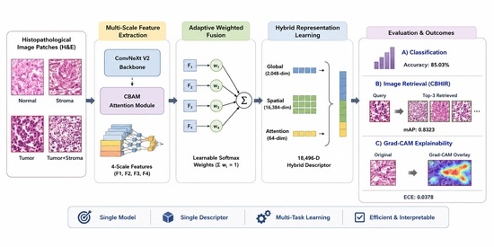
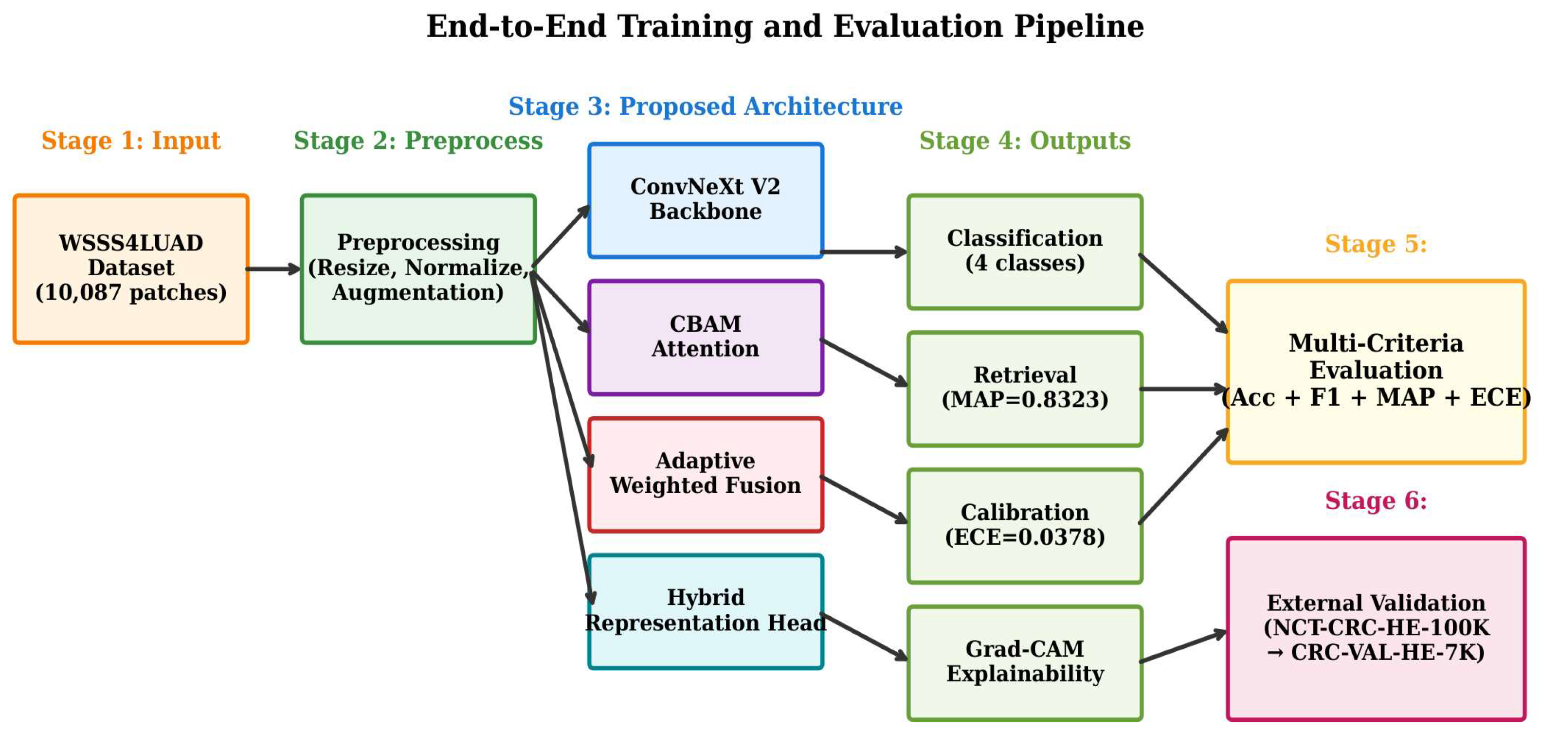
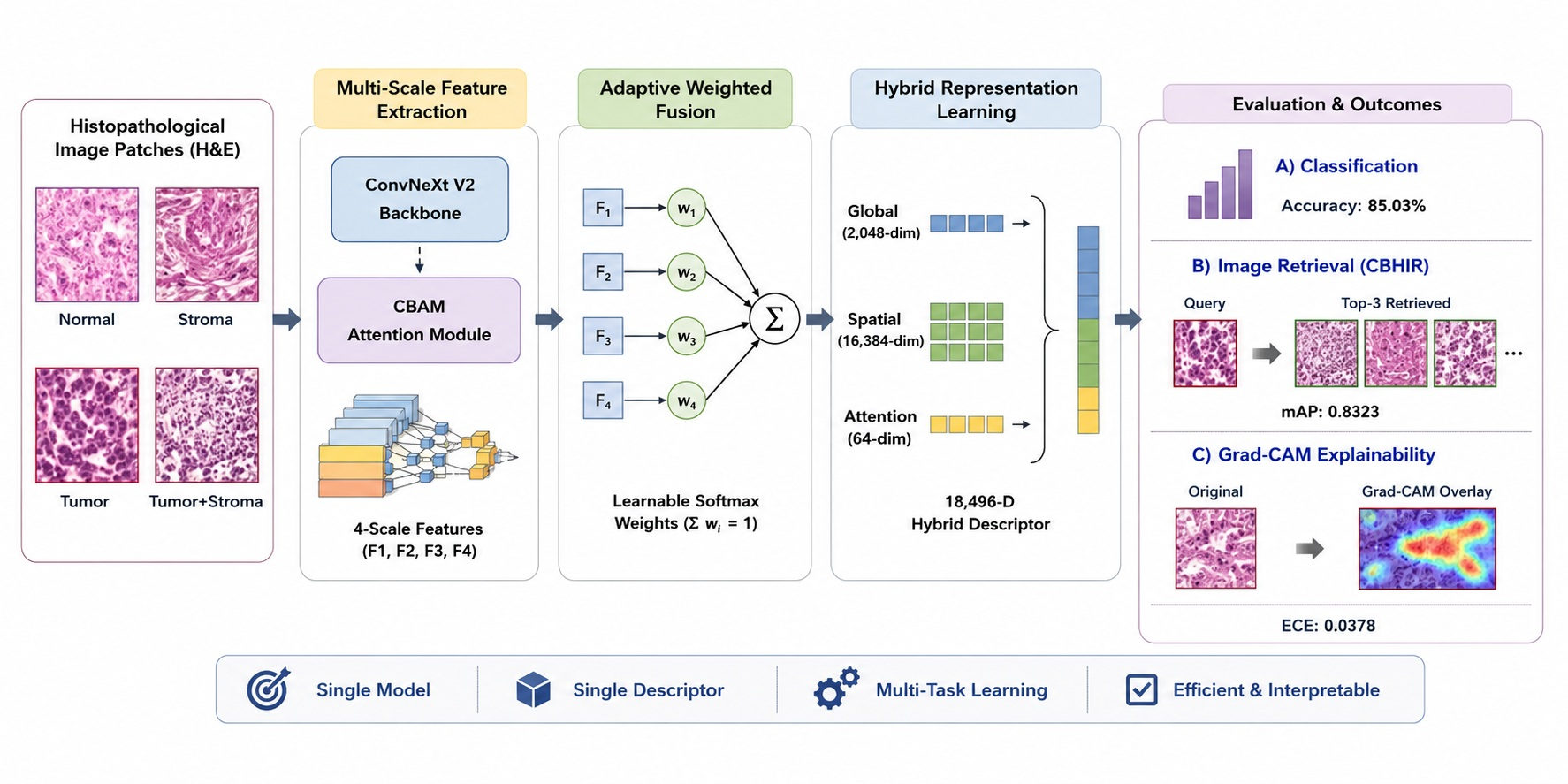
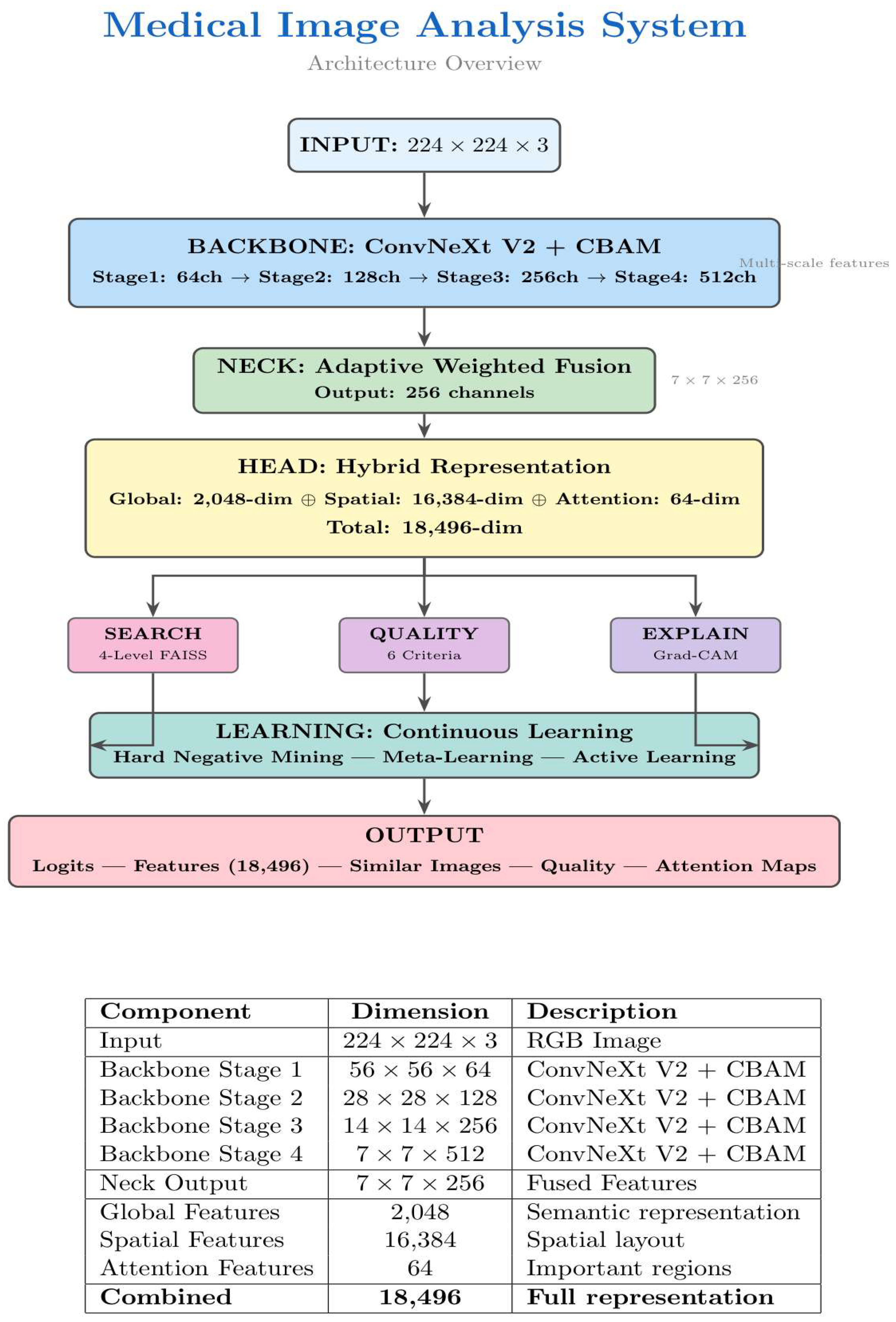
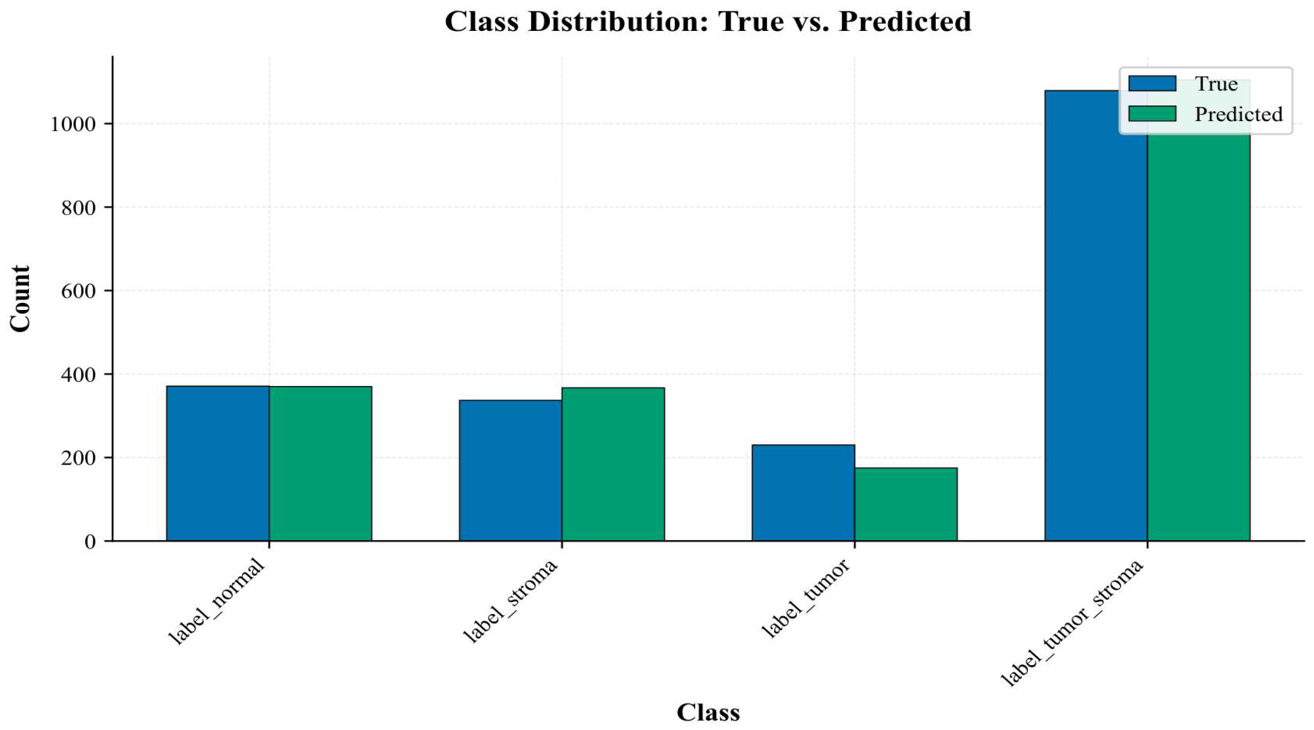
End-to-end training and evaluation pipeline of the proposed framework. The six stages cover: (1) input data preparation from WSSS4LUAD, (2) preprocessing with augmentation, (3) the proposed architecture with four components (ConvNeXt V2, CBAM, Adaptive Weighted Fusion, Hybrid Head), (4) four output capabilities (classification, retrieval, calibration, Grad-CAM), (5) multi-criteria evaluation, and (6) external validation on an independent dataset.
Figure 2.
End-to-end training and evaluation pipeline of the proposed framework. The six stages cover: (1) input data preparation from WSSS4LUAD, (2) preprocessing with augmentation, (3) the proposed architecture with four components (ConvNeXt V2, CBAM, Adaptive Weighted Fusion, Hybrid Head), (4) four output capabilities (classification, retrieval, calibration, Grad-CAM), (5) multi-criteria evaluation, and (6) external validation on an independent dataset.
Figure 3.
Class distribution of the WSSS4LUAD dataset. The dataset exhibits significant class imbalance, with Tumor-Stroma comprising 53.48% of all samples and Tumor being the least represented class at 11.71%.
Figure 3.
Class distribution of the WSSS4LUAD dataset. The dataset exhibits significant class imbalance, with Tumor-Stroma comprising 53.48% of all samples and Tumor being the least represented class at 11.71%.
Figure 4.
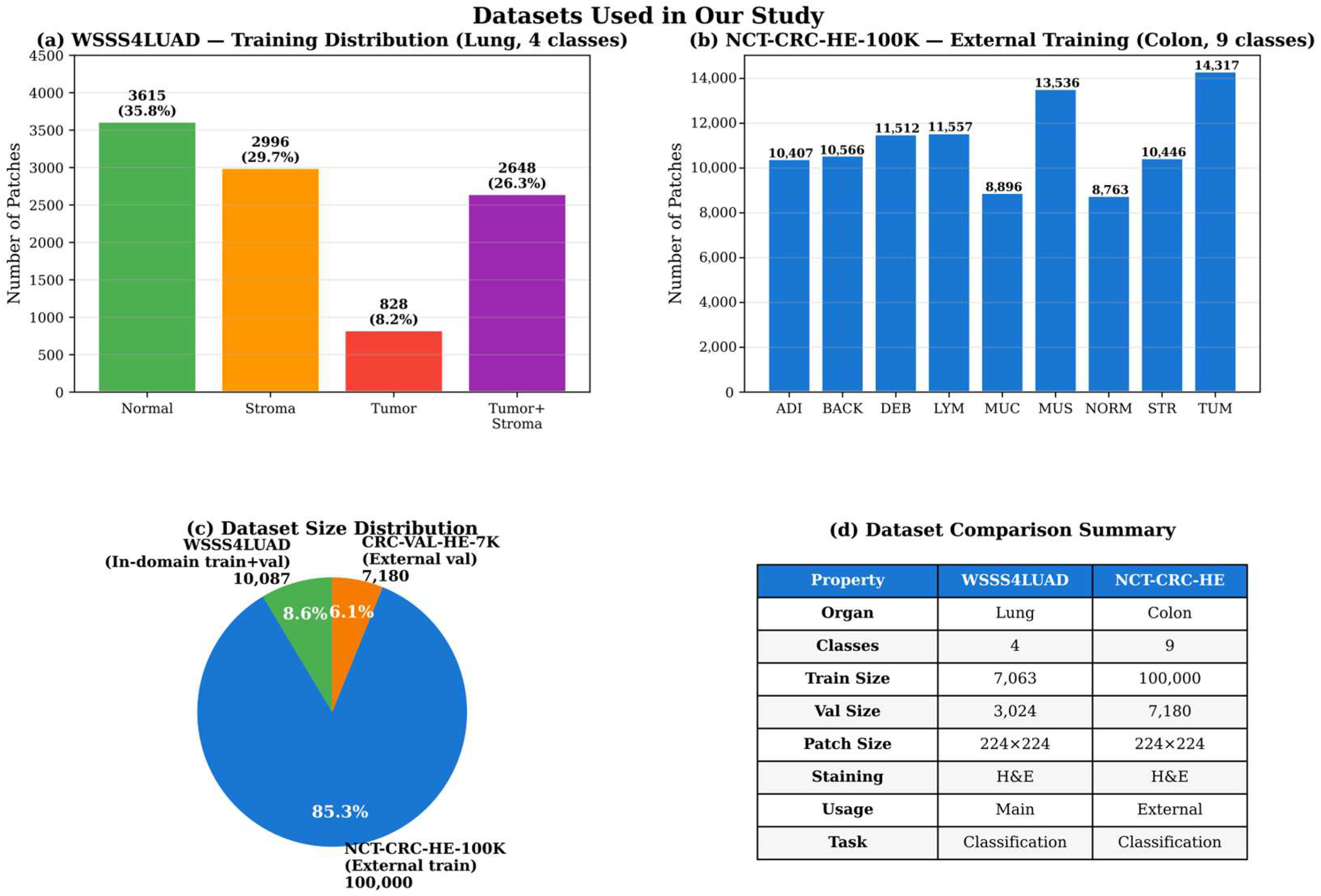
Overview of the datasets used in our study. (a) WSSS4LUAD class distribution (classes, lung tissue). (b) NCT-CRC-HE-100K class distribution (classes, colon tissue) used for external validation. (c) Proportional size comparison across the three dataset splits. (d) Side-by-side comparison of key dataset properties, highlighting cross-organ generalization (lung colon) and increased class complexity (4 9 classes).
Figure 4.
Overview of the datasets used in our study. (a) WSSS4LUAD class distribution (classes, lung tissue). (b) NCT-CRC-HE-100K class distribution (classes, colon tissue) used for external validation. (c) Proportional size comparison across the three dataset splits. (d) Side-by-side comparison of key dataset properties, highlighting cross-organ generalization (lung colon) and increased class complexity (4 9 classes).
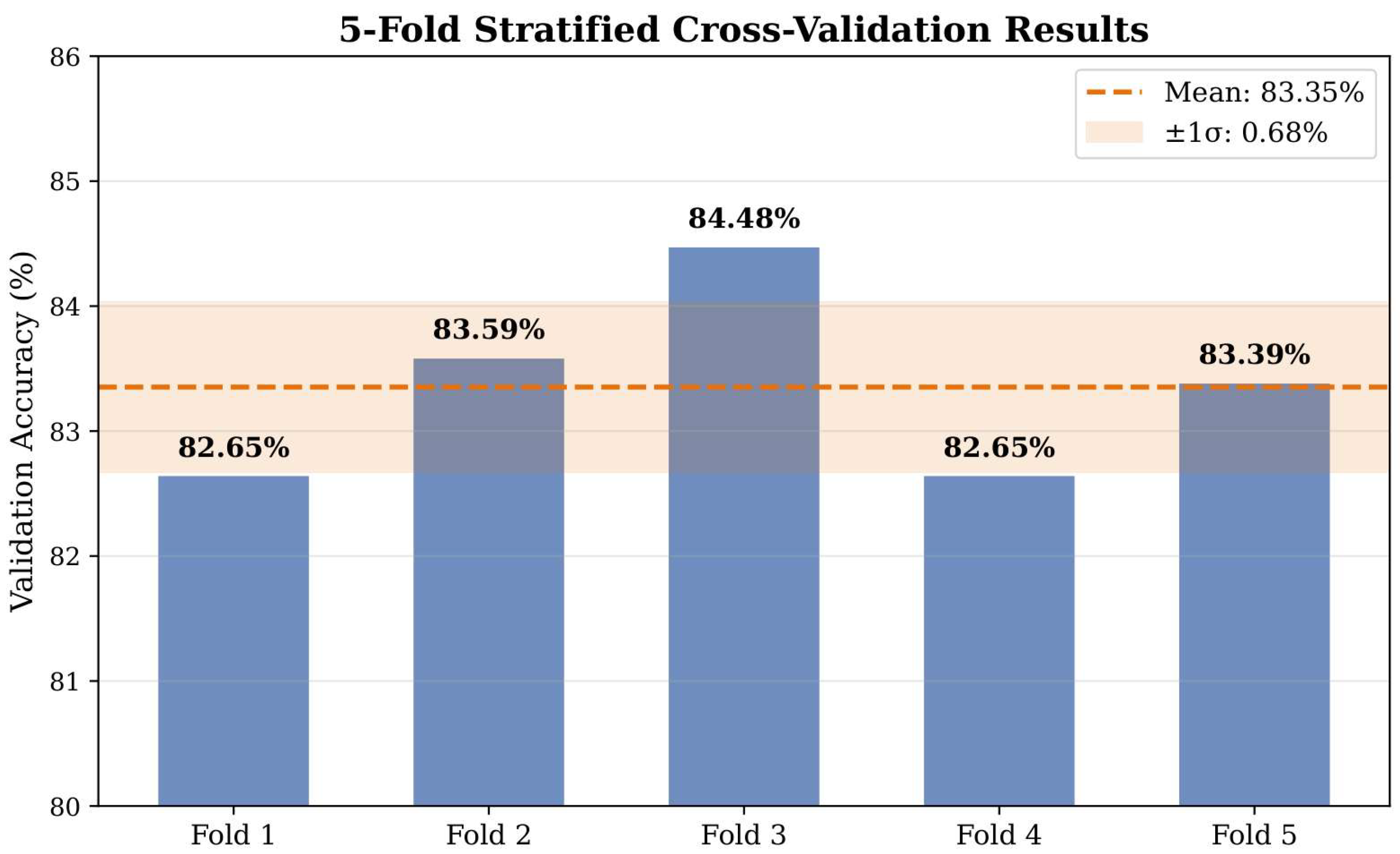
Figure 6.
5-fold stratified cross-validation results. The orange dashed line indicates the mean accuracy (83.35%), and the shaded band represents standard deviation (0.93%), demonstrating high consistency across data partitions.
Figure 6.
5-fold stratified cross-validation results. The orange dashed line indicates the mean accuracy (83.35%), and the shaded band represents standard deviation (0.93%), demonstrating high consistency across data partitions.
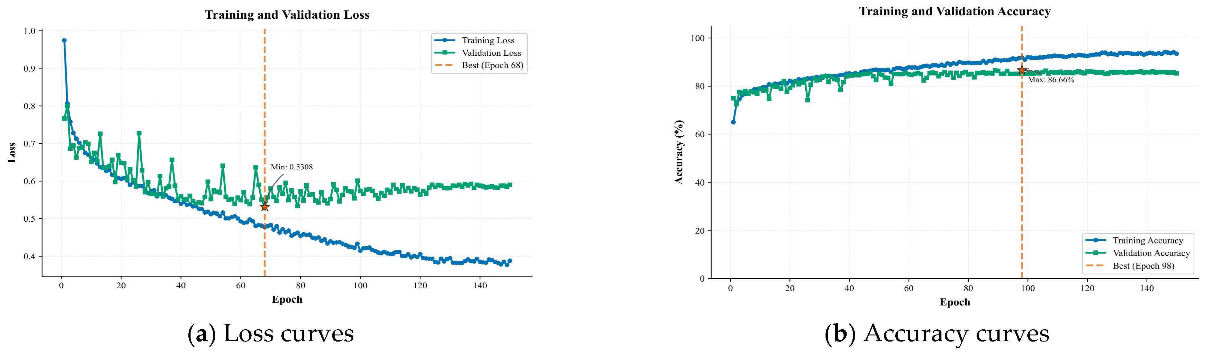
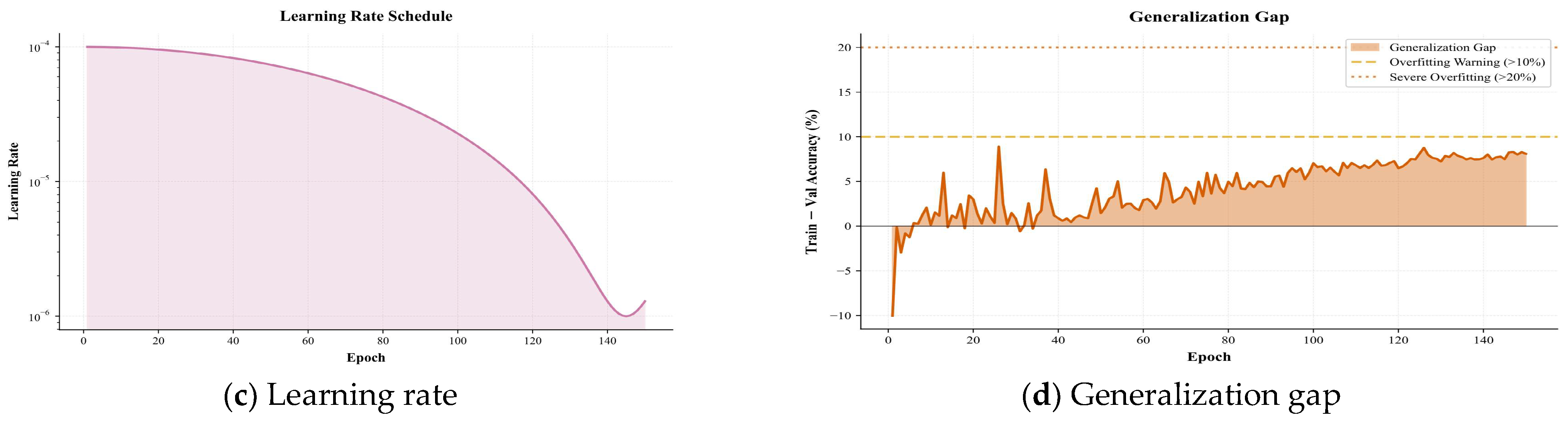
Figure 7.
Training dynamics over 150 epochs. (a) Training and validation loss curves showing convergence. (b) Training and validation accuracy curves; best validation accuracy of 86.66% at epoch 98. (c) Cosine annealing learning rate schedule with epoch linear warmup. (d) Generalization gap stabilizing at approximately 7–8% after epoch 100.
Figure 7.
Training dynamics over 150 epochs. (a) Training and validation loss curves showing convergence. (b) Training and validation accuracy curves; best validation accuracy of 86.66% at epoch 98. (c) Cosine annealing learning rate schedule with epoch linear warmup. (d) Generalization gap stabilizing at approximately 7–8% after epoch 100.
Figure 8.
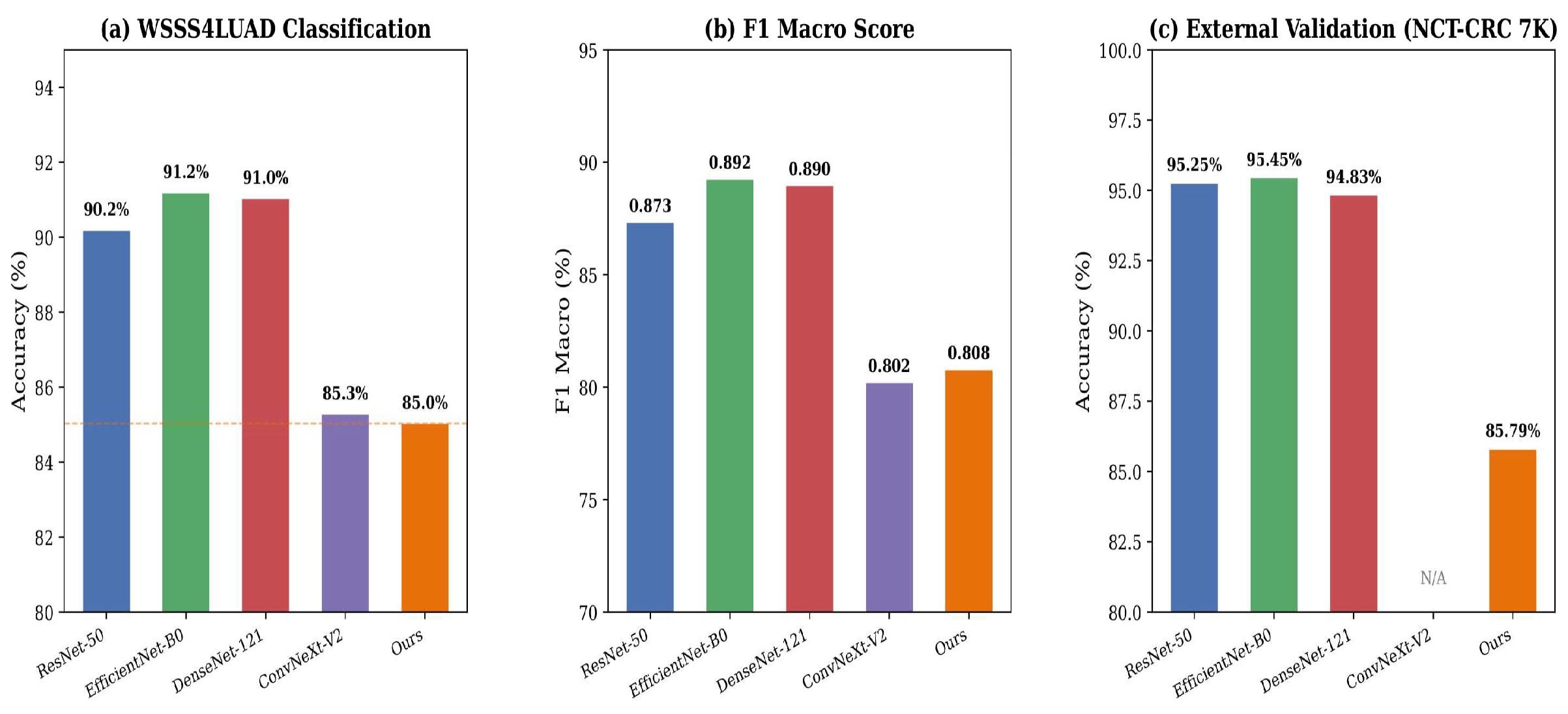
Three evaluation dimensions, grouped comparison. (a) WSSS4LUAD accuracy: baselines lead by 5–6%, (b) F1 macro scores, and (c) external validation on CRC-VAL-HE-7K, where baselines (trained on 100 K) achieve 94% and our model (trained on 10.8 K) achieves 85.79%. N/A indicates that external validation was not performed for the vanilla ConvNeXt-V2 baseline; therefore, no corresponding accuracy is reported.
Figure 8.
Three evaluation dimensions, grouped comparison. (a) WSSS4LUAD accuracy: baselines lead by 5–6%, (b) F1 macro scores, and (c) external validation on CRC-VAL-HE-7K, where baselines (trained on 100 K) achieve 94% and our model (trained on 10.8 K) achieves 85.79%. N/A indicates that external validation was not performed for the vanilla ConvNeXt-V2 baseline; therefore, no corresponding accuracy is reported.
Figure 9.
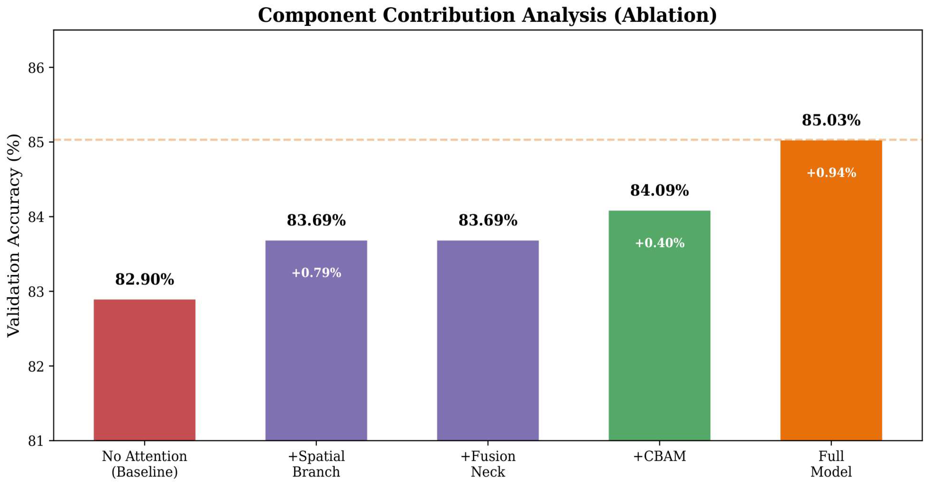
Component contribution analysis. Starting from the baseline configuration without attention (82.90%), each module incrementally improves the classification accuracy, with the complete model reaching (85.03%) (+2.13% overall improvement).
Figure 9.
Component contribution analysis. Starting from the baseline configuration without attention (82.90%), each module incrementally improves the classification accuracy, with the complete model reaching (85.03%) (+2.13% overall improvement).
Figure 10.
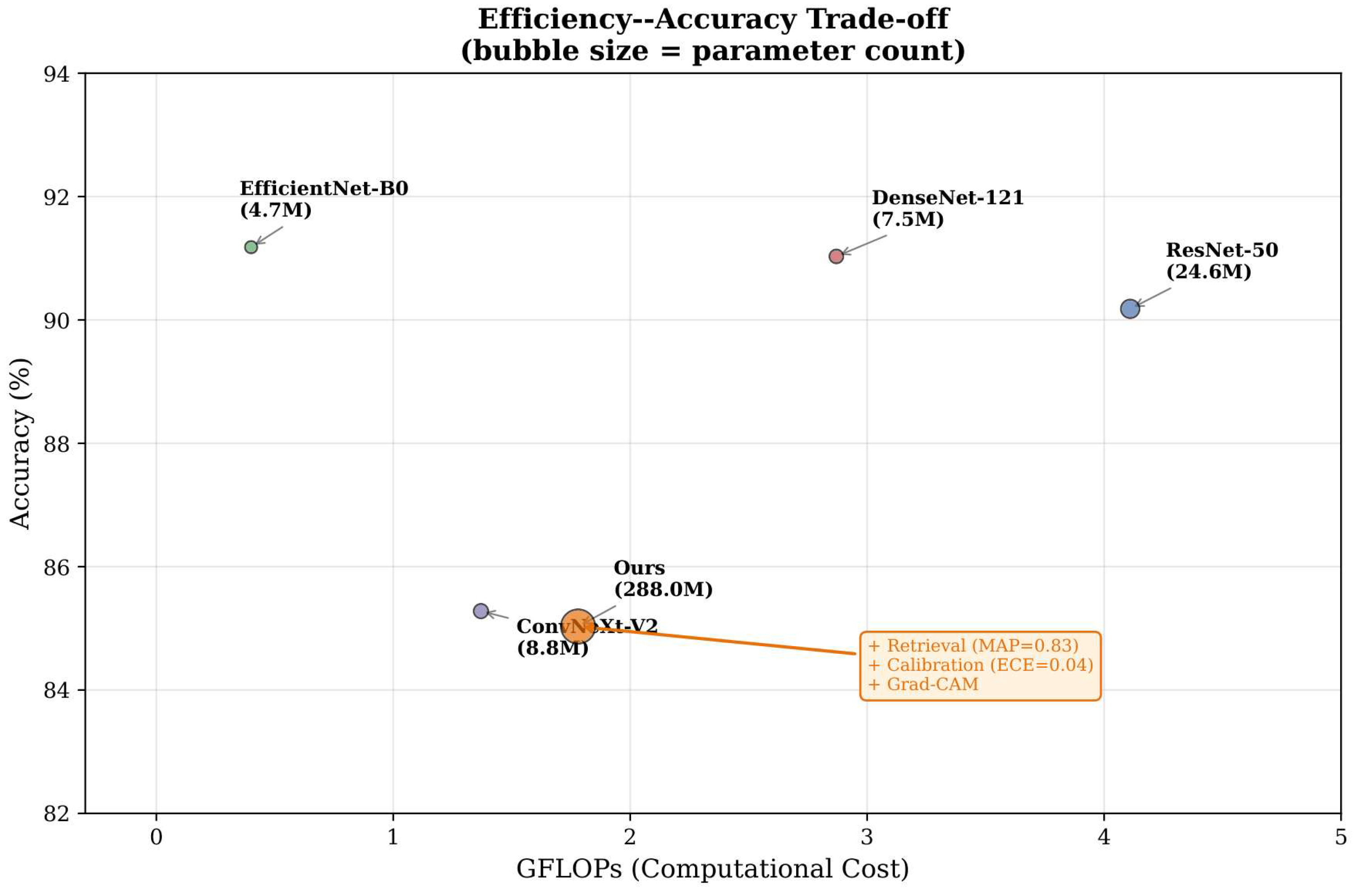
Efficiency–accuracy trade-off. The size of the bubbles corresponds to the number of parameters. Our model achieves similar GFLOPs to lightweight baselines while offering retrieval. (MAP ), calibration (ECE ), and Grad-CAM functionality.
Figure 10.
Efficiency–accuracy trade-off. The size of the bubbles corresponds to the number of parameters. Our model achieves similar GFLOPs to lightweight baselines while offering retrieval. (MAP ), calibration (ECE ), and Grad-CAM functionality.
Figure 11.
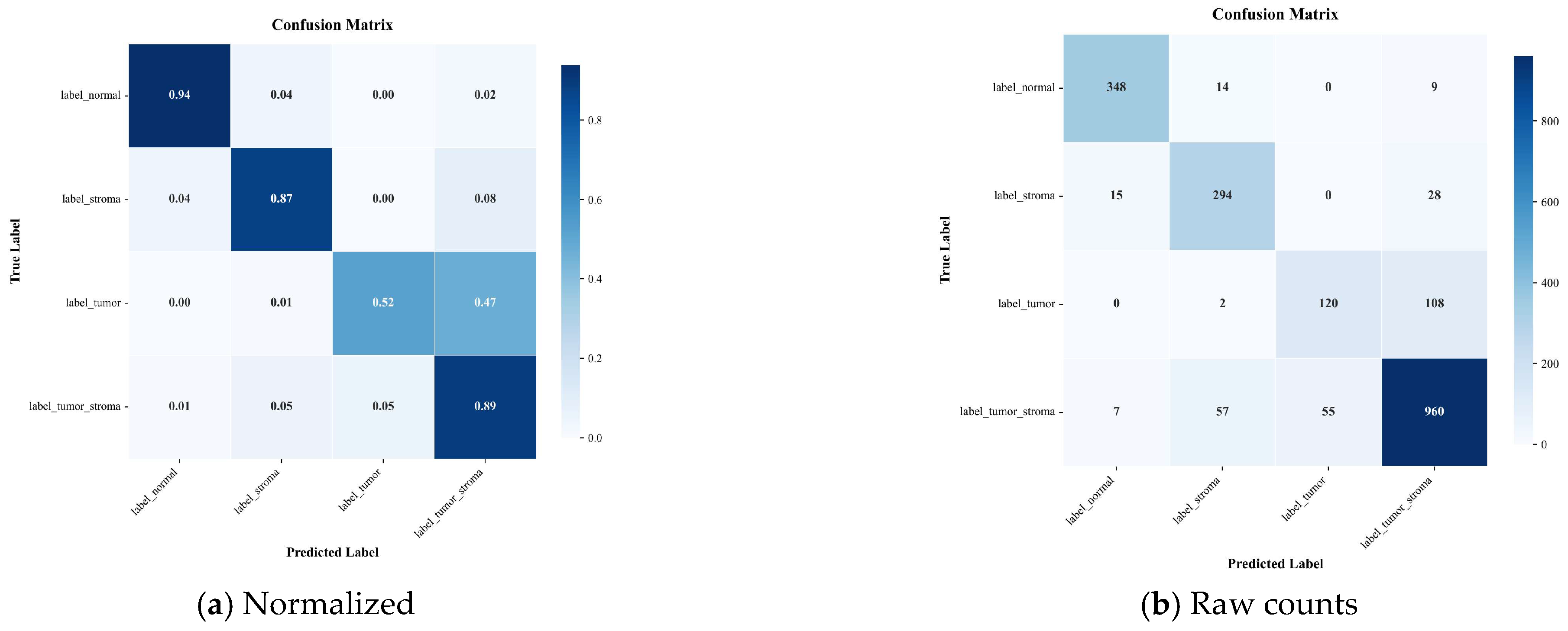
Confusion matrices obtained on the WSSS4LUAD validation set. (a) Normalized confusion matrix illustrating the per-class accuracy percentages. (b) Raw confusion matrix presenting the absolute prediction counts.
Figure 11.
Confusion matrices obtained on the WSSS4LUAD validation set. (a) Normalized confusion matrix illustrating the per-class accuracy percentages. (b) Raw confusion matrix presenting the absolute prediction counts.
Figure 12.
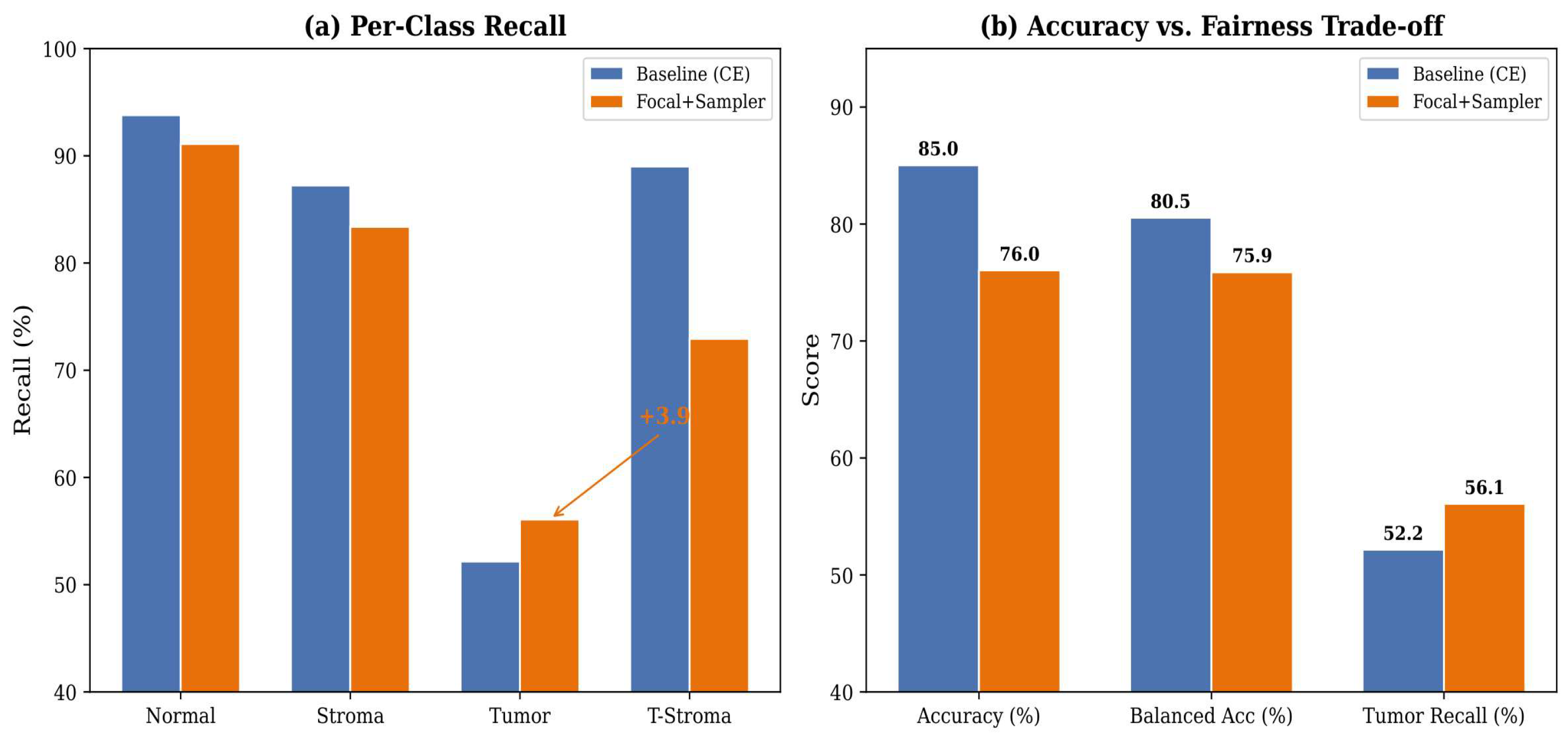
Class-balancing analysis. (a) Per-class recall: Focal+Sampler improves Tumor recall (+3.92%) at the expense of Tumor-Stroma recall (). (b) Overall accuracy drops from 85.03% to 76.05%, illustrating the accuracy–fairness trade-off.
Figure 12.
Class-balancing analysis. (a) Per-class recall: Focal+Sampler improves Tumor recall (+3.92%) at the expense of Tumor-Stroma recall (). (b) Overall accuracy drops from 85.03% to 76.05%, illustrating the accuracy–fairness trade-off.
Figure 13.
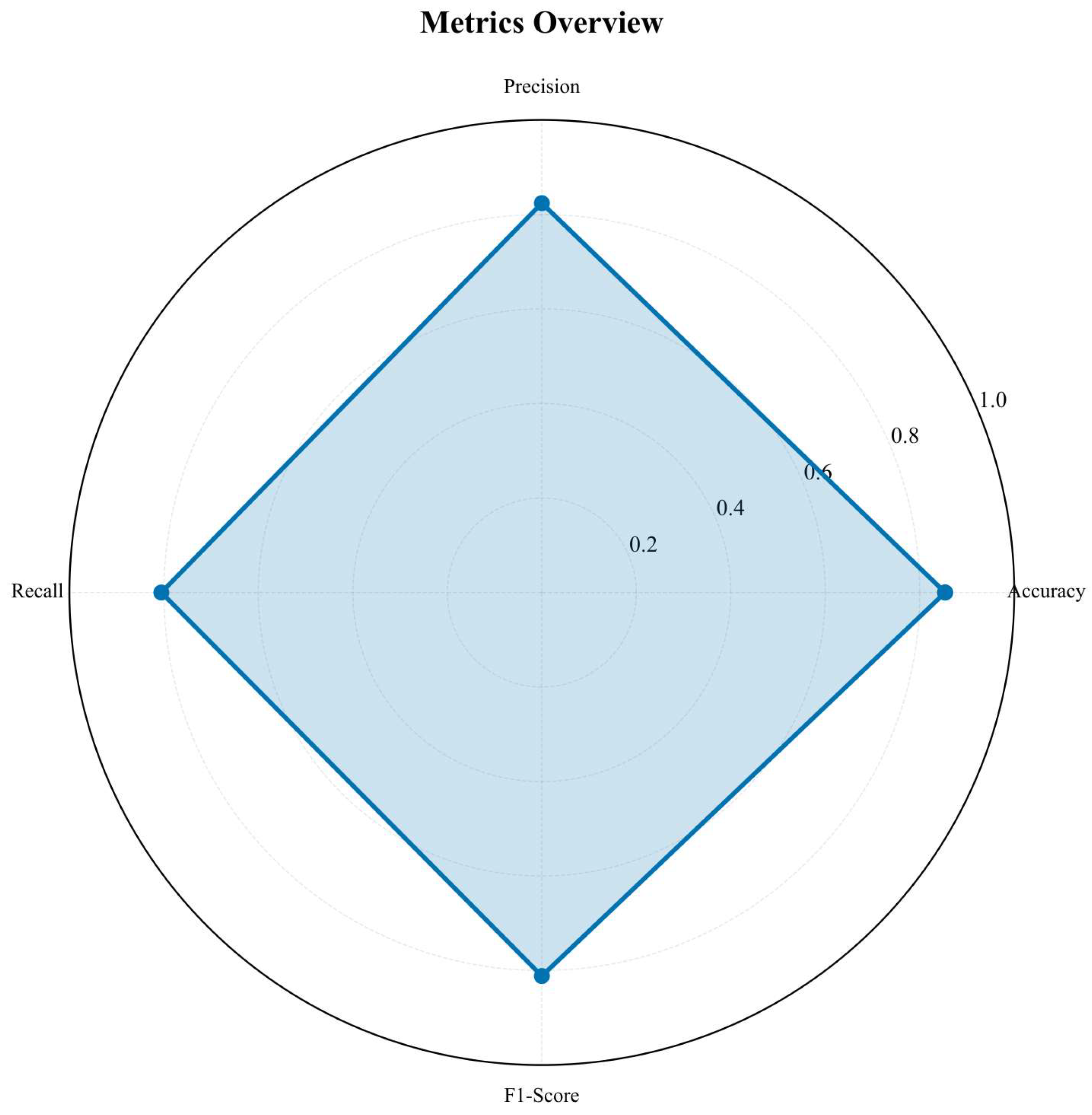
Radar chart of per-class classification metrics. Normal tissue achieves the most balanced and highest performance across all metrics, while Tumor shows the largest gap between precision and recall.
Figure 13.
Radar chart of per-class classification metrics. Normal tissue achieves the most balanced and highest performance across all metrics, while Tumor shows the largest gap between precision and recall.
Figure 14.
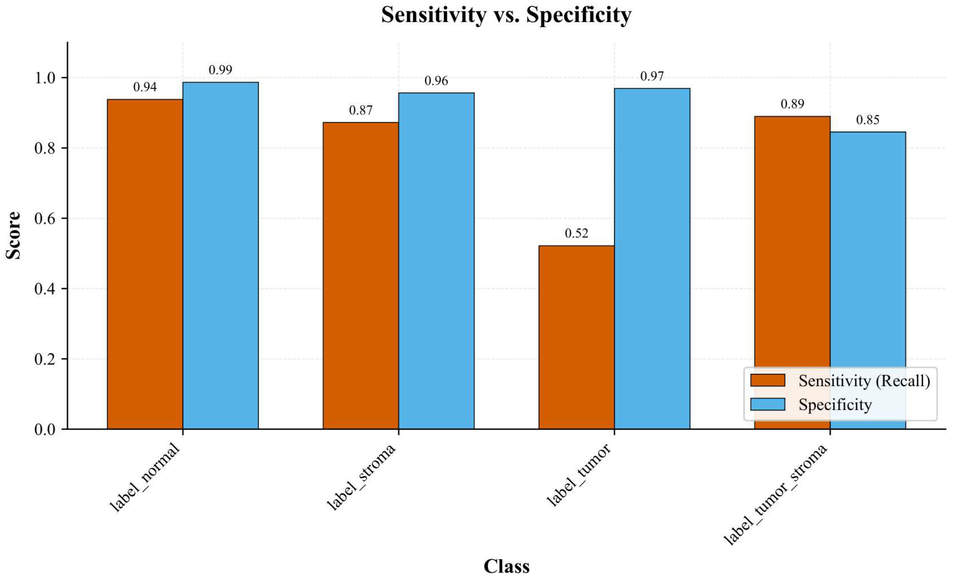
Sensitivity and specificity comparison across tissue classes. All classes achieve specificity above 0.84, with Normal tissue reaching 0.99. The Tumor class shows the largest sensitivity–specificity gap.
Figure 14.
Sensitivity and specificity comparison across tissue classes. All classes achieve specificity above 0.84, with Normal tissue reaching 0.99. The Tumor class shows the largest sensitivity–specificity gap.
Figure 15.
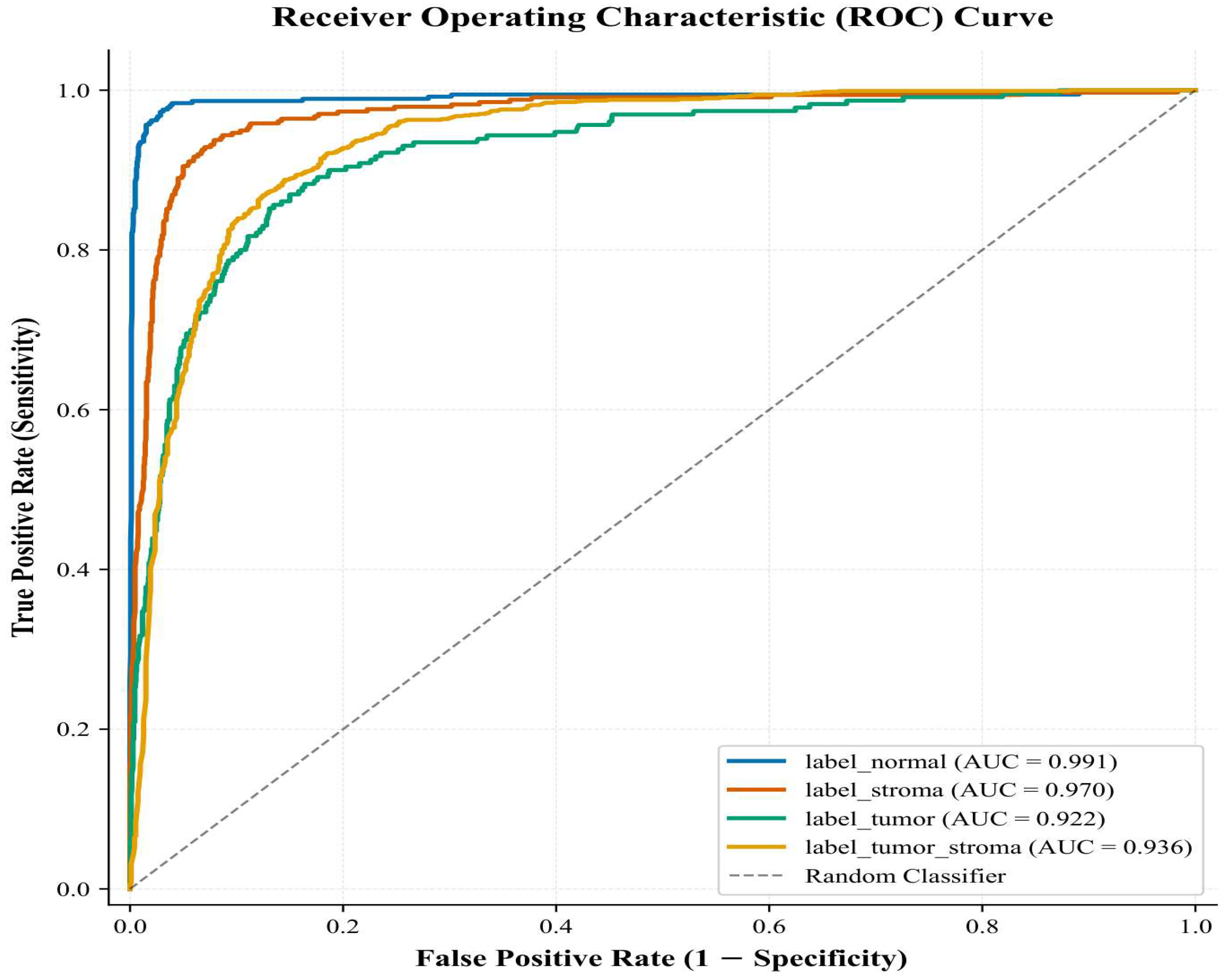
Receiver Operating Characteristic (ROC) curves for each tissue class. The area under the curve (AUC) is highest for Normal tissue and lowest for the Tumor.
Figure 15.
Receiver Operating Characteristic (ROC) curves for each tissue class. The area under the curve (AUC) is highest for Normal tissue and lowest for the Tumor.
Figure 16.
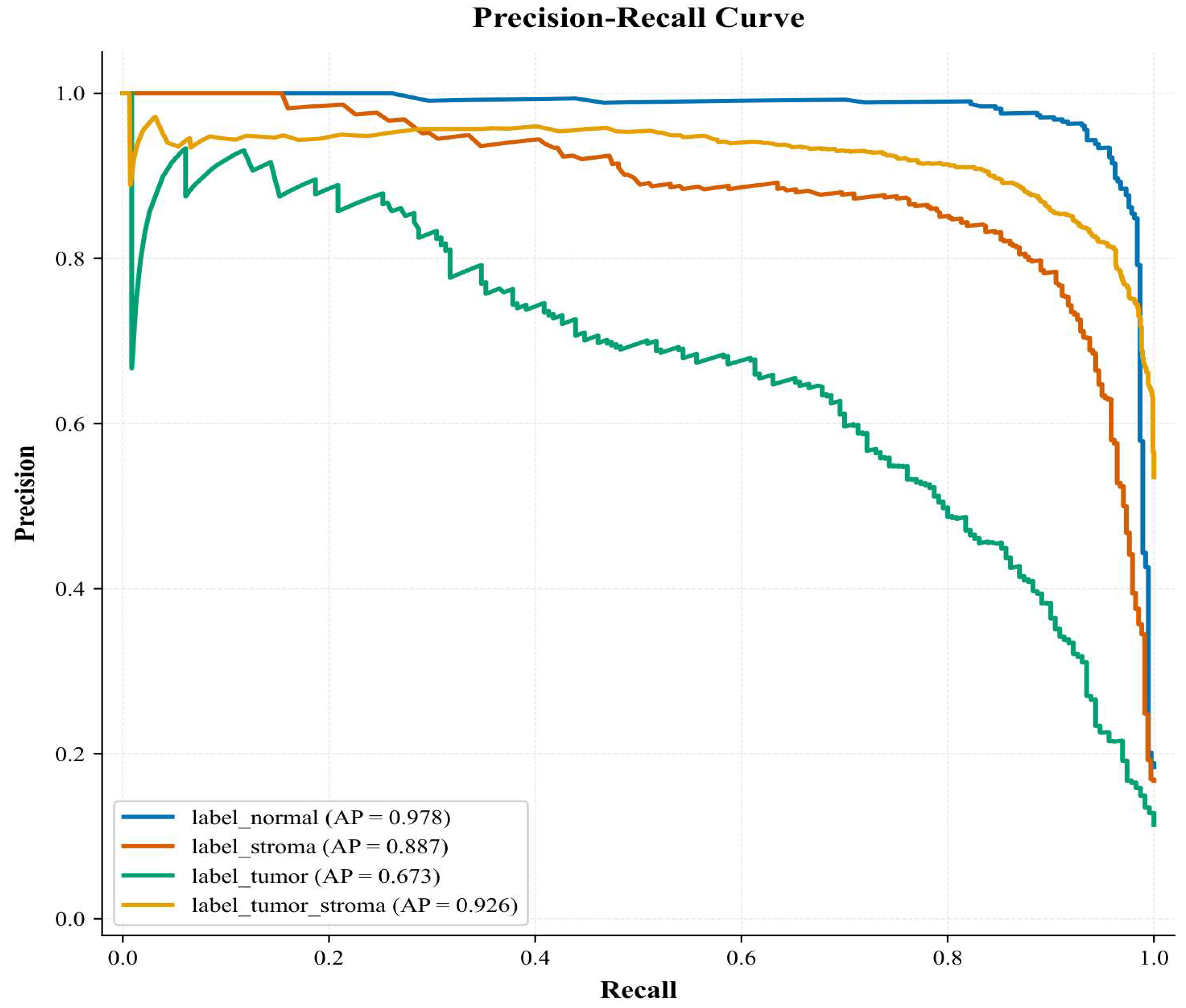
Precision–Recall curves for each tissue class. The curves reflect the trade-off between precision and recall, with Normal tissue maintaining the highest AP.
Figure 16.
Precision–Recall curves for each tissue class. The curves reflect the trade-off between precision and recall, with Normal tissue maintaining the highest AP.
Figure 17.
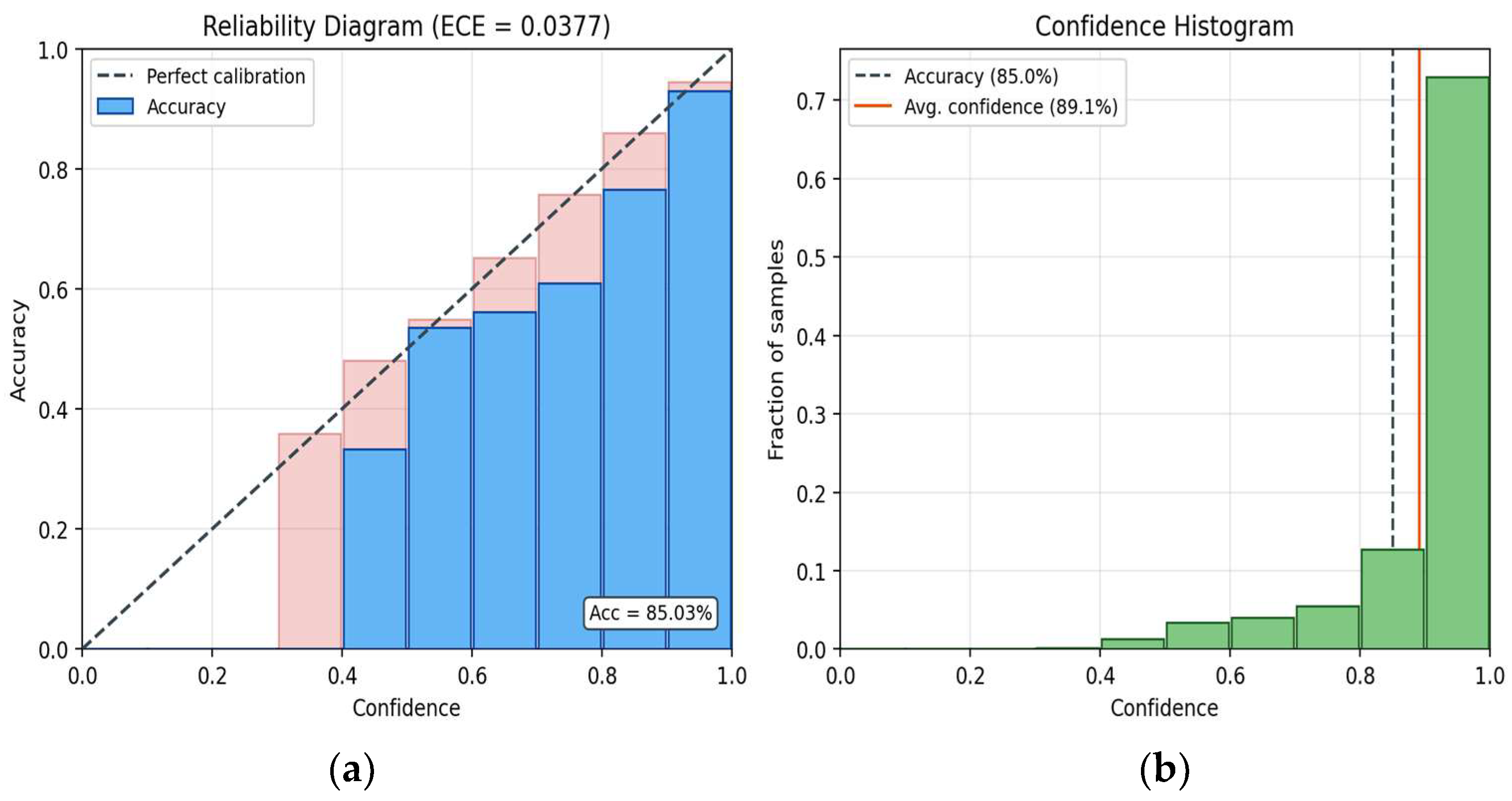
Calibration analysis on the WSSS4LUAD validation set. (a) Reliability diagram (10 bins): blue bars are per-bin accuracy, red bars show the gap to the diagonal (perfect calibration); the overall ECE is 0.0377. (b) Confidence histogram: the dashed line marks overall accuracy (85.0%) and the solid line marks mean confidence (89.1%), indicating mild over-confidence. No temperature scaling was applied; calibration is obtained intrinsically through label smoothing.
Figure 17.
Calibration analysis on the WSSS4LUAD validation set. (a) Reliability diagram (10 bins): blue bars are per-bin accuracy, red bars show the gap to the diagonal (perfect calibration); the overall ECE is 0.0377. (b) Confidence histogram: the dashed line marks overall accuracy (85.0%) and the solid line marks mean confidence (89.1%), indicating mild over-confidence. No temperature scaling was applied; calibration is obtained intrinsically through label smoothing.
Figure 18.
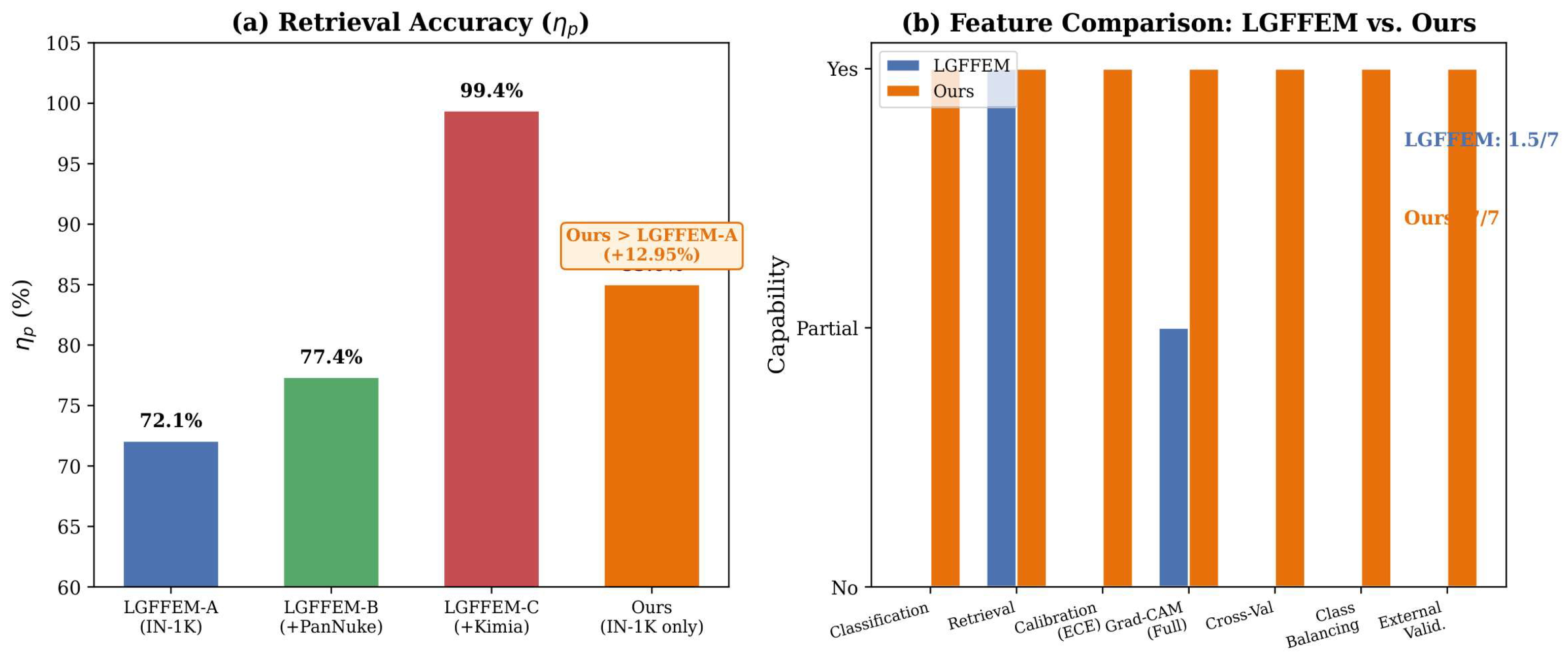
LGFFEM vs. Ours. (a) Retrieval accuracy: the proposed model achieves (85.03%) accuracy, exceeding the (72.08%) obtained by the ImageNet-only LGFFEM-A model by +12.95%, (b) Capability comparison: our framework provides 7/7 capabilities vs. 1.5/7 for LGFFEM.
Figure 18.
LGFFEM vs. Ours. (a) Retrieval accuracy: the proposed model achieves (85.03%) accuracy, exceeding the (72.08%) obtained by the ImageNet-only LGFFEM-A model by +12.95%, (b) Capability comparison: our framework provides 7/7 capabilities vs. 1.5/7 for LGFFEM.
Figure 19.
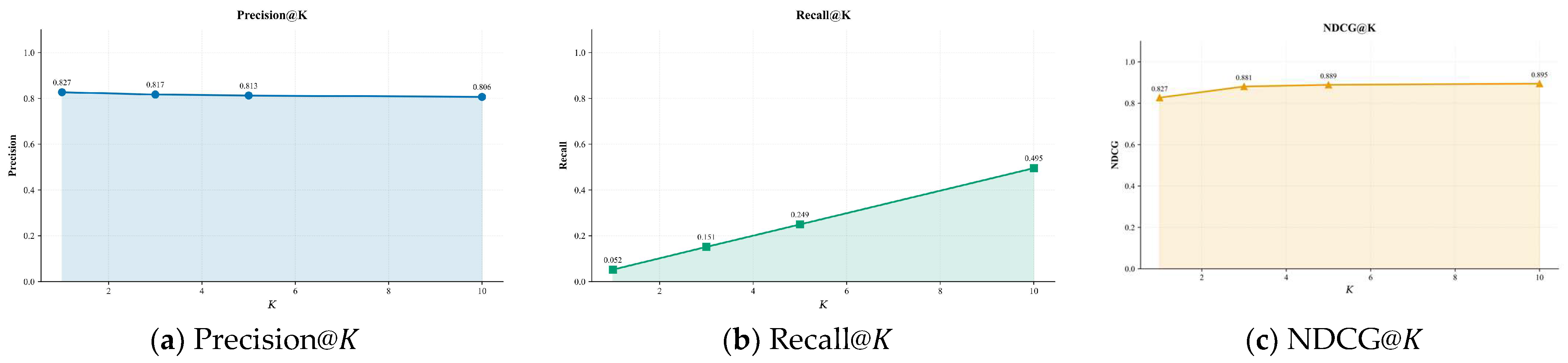
Retrieval performance metrics at different values of . (a) Precision@ shows a gradual decline as increases, indicating that relevant images are concentrated at the top of the ranked list. (b) Recall@ rises as , increases as the more images being covered are relevant. (c) The greater NDCG@K is, the higher the ranking quality is, and it grows as K increases.
Figure 19.
Retrieval performance metrics at different values of . (a) Precision@ shows a gradual decline as increases, indicating that relevant images are concentrated at the top of the ranked list. (b) Recall@ rises as , increases as the more images being covered are relevant. (c) The greater NDCG@K is, the higher the ranking quality is, and it grows as K increases.
Figure 20.
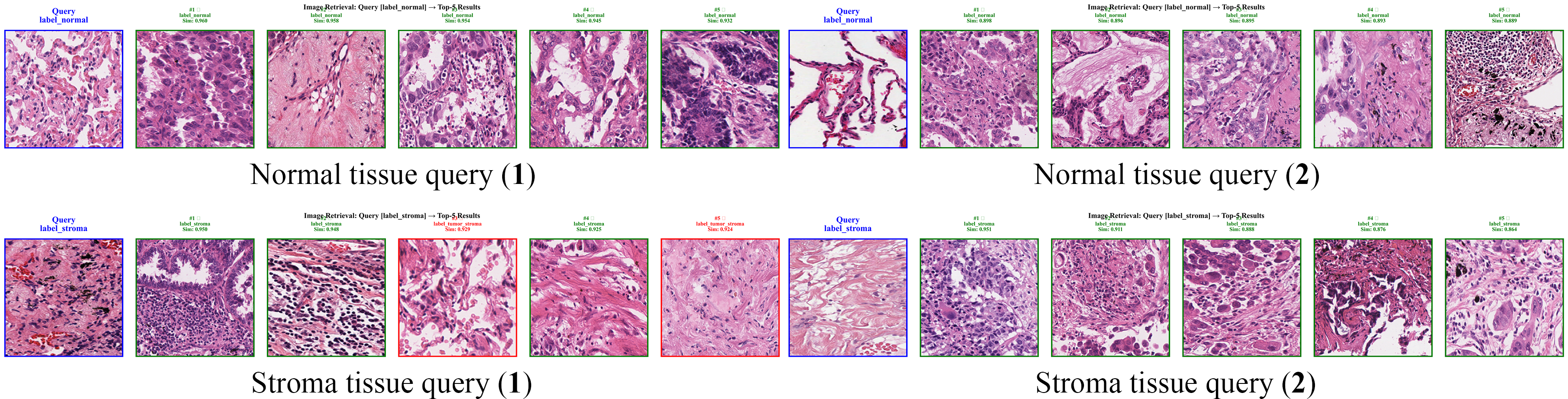
Qualitative retrieval examples for the Normal and Stroma tissue classes. Each row presents two independent retrieval examples. For each example, the leftmost image is the query image, followed by its top- retrieved results. Green borders indicate correct retrievals, red borders indicate incorrect ones.
Figure 20.
Qualitative retrieval examples for the Normal and Stroma tissue classes. Each row presents two independent retrieval examples. For each example, the leftmost image is the query image, followed by its top- retrieved results. Green borders indicate correct retrievals, red borders indicate incorrect ones.
Figure 21.
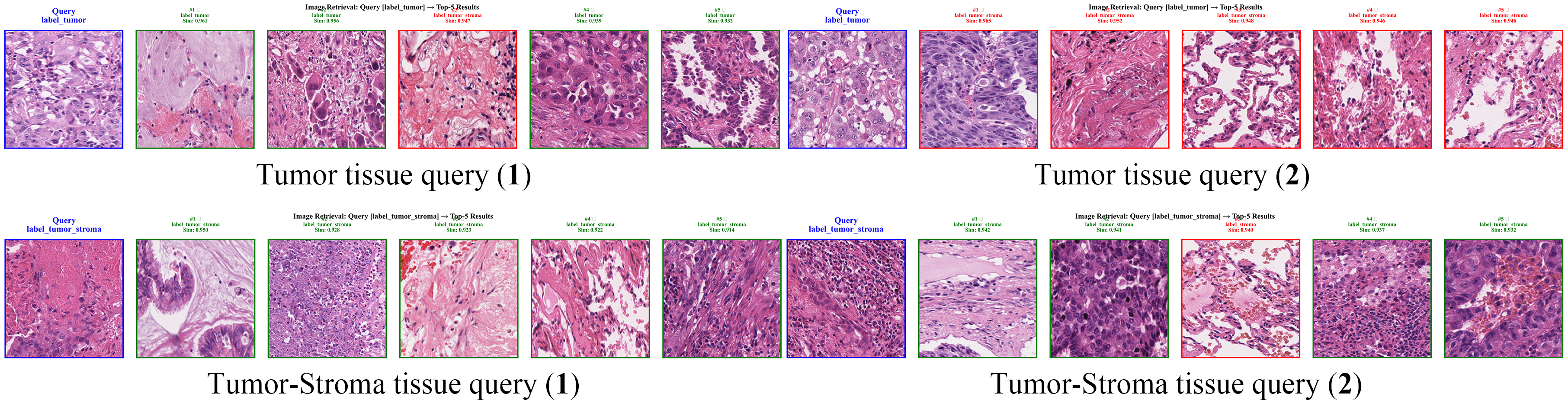
Qualitative retrieval examples for Tumor and Tumor-Stroma tissue classes. Each panel shows the query image (left) and its top-5 retrieved results. Green borders indicate correct retrievals, red borders indicate incorrect ones.
Figure 21.
Qualitative retrieval examples for Tumor and Tumor-Stroma tissue classes. Each panel shows the query image (left) and its top-5 retrieved results. Green borders indicate correct retrievals, red borders indicate incorrect ones.
Figure 22.
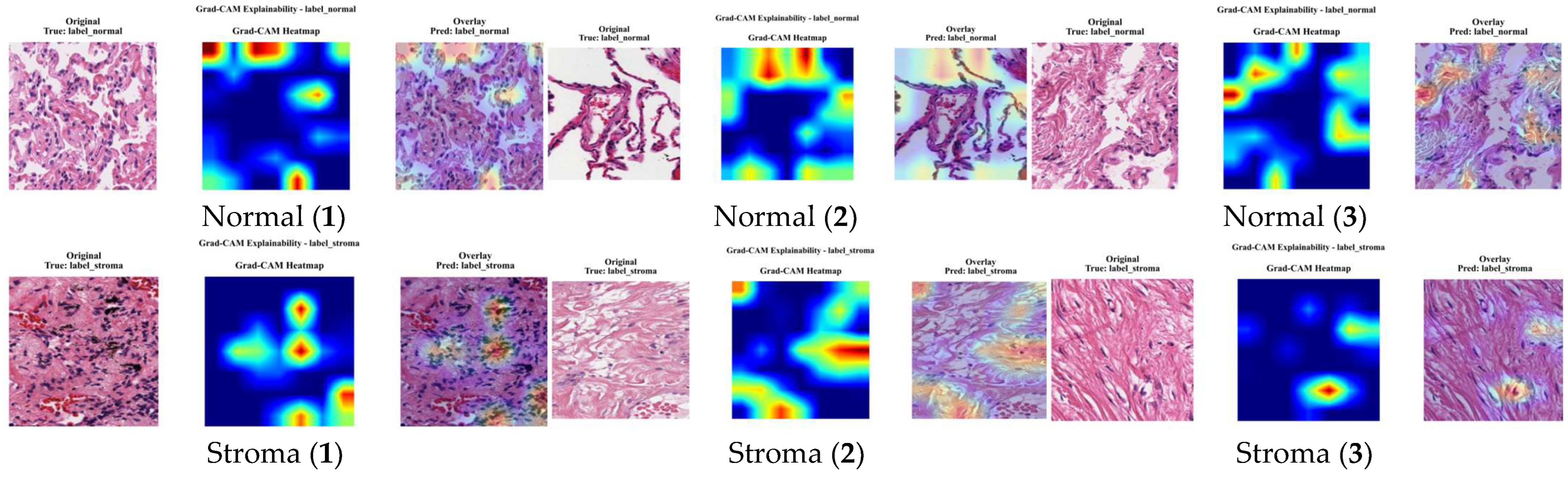
Grad-CAM visualizations for Normal and Stroma tissue classes (3 samples each). In normal tissue, attention is diffuse in the alveolar space, while in the stroma, attention is concentrated on the connective tissue fibers.
Figure 22.
Grad-CAM visualizations for Normal and Stroma tissue classes (3 samples each). In normal tissue, attention is diffuse in the alveolar space, while in the stroma, attention is concentrated on the connective tissue fibers.
Figure 23.
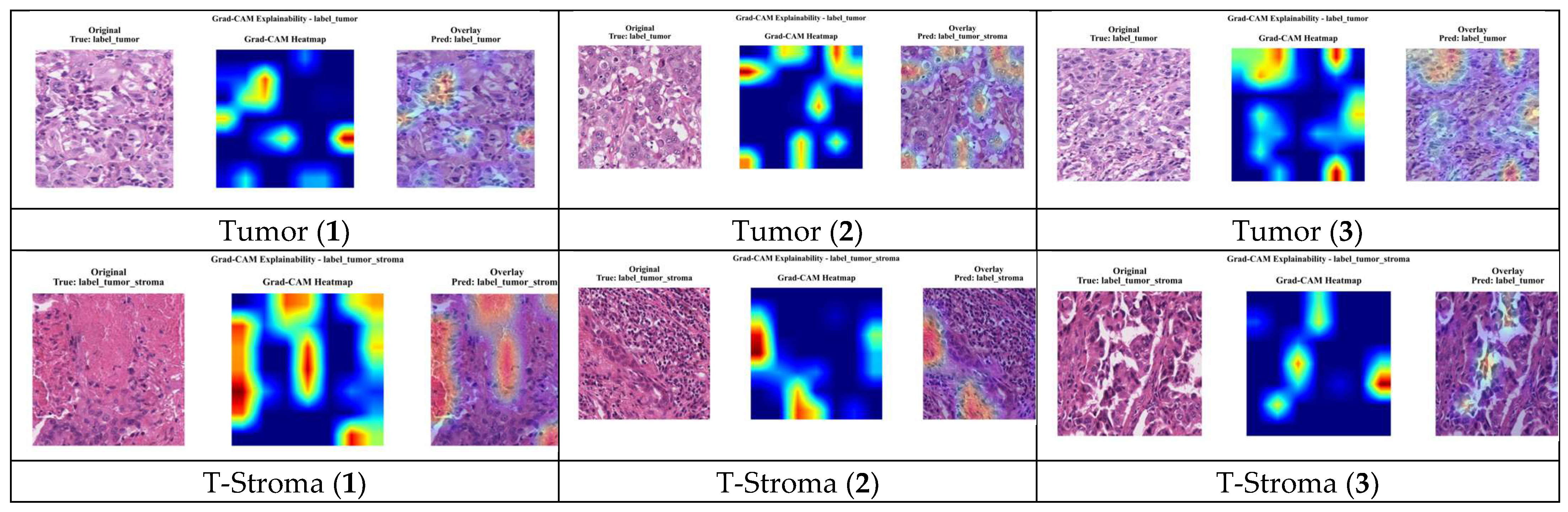
Grad-CAM visualizations for Tumor and Tumor-Stroma tissue classes (3 samples each). Tumor highlights clusters of abnormal cells, and Tumor-Stroma demonstrates dual attention to both epithelial and stromal parts.
Figure 23.
Grad-CAM visualizations for Tumor and Tumor-Stroma tissue classes (3 samples each). Tumor highlights clusters of abnormal cells, and Tumor-Stroma demonstrates dual attention to both epithelial and stromal parts.
Figure 24.
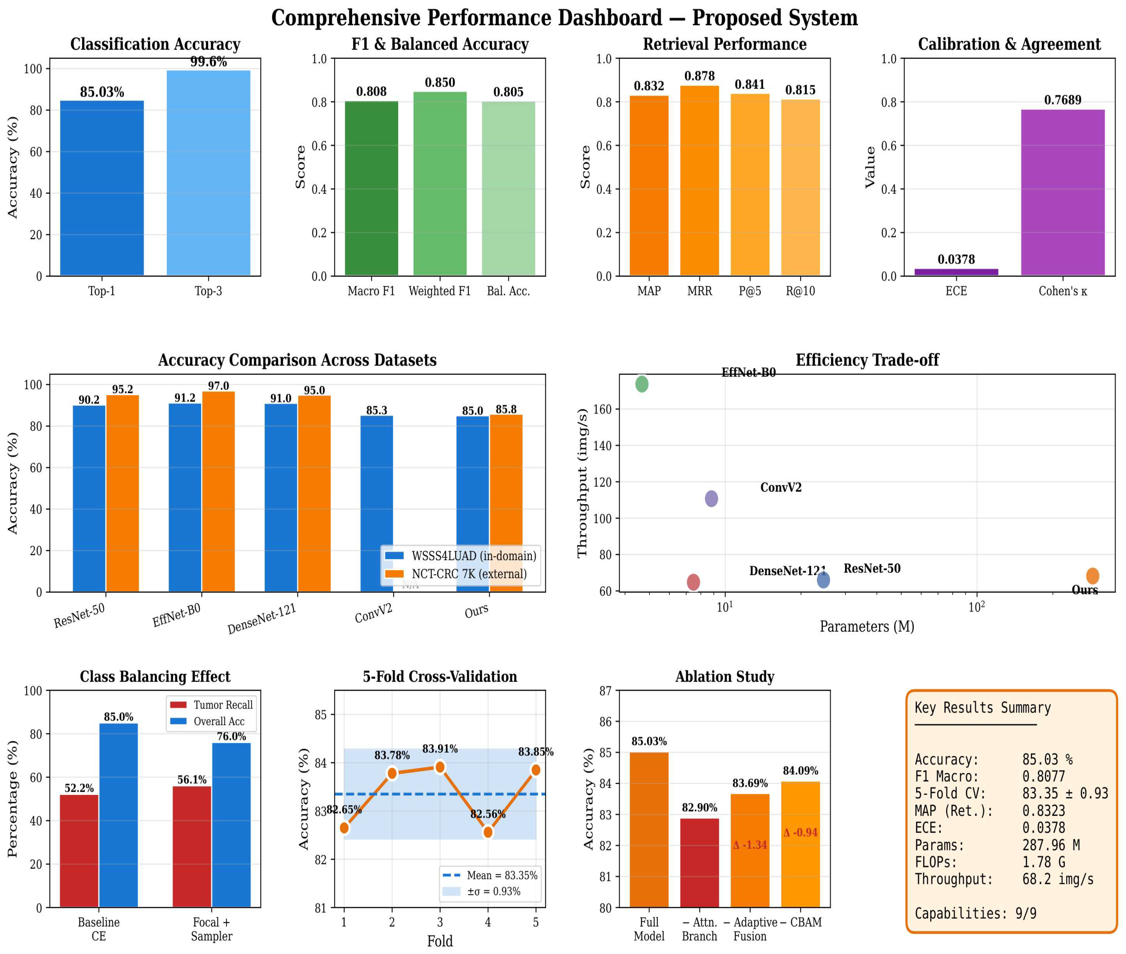
Proposed system comprehensive performance dashboard. Left column: classification accuracy, F1 scores, retrieval measures, and calibration measures. In the middle row: accuracy comparison between in-domain data WSSS4LUAD and external data NCT-CRC-HE-7K and efficiency trade-off between parameters and throughput. The bottom row shows the class balancing effect, 5-fold cross validation stability, ablation study, and key results summary. N/A indicates that ConvNeXt-V2 was evaluated only on the WSSS4LUAD dataset; therefore, no external validation results is available.
Figure 24.
Proposed system comprehensive performance dashboard. Left column: classification accuracy, F1 scores, retrieval measures, and calibration measures. In the middle row: accuracy comparison between in-domain data WSSS4LUAD and external data NCT-CRC-HE-7K and efficiency trade-off between parameters and throughput. The bottom row shows the class balancing effect, 5-fold cross validation stability, ablation study, and key results summary. N/A indicates that ConvNeXt-V2 was evaluated only on the WSSS4LUAD dataset; therefore, no external validation results is available.
Figure 25.
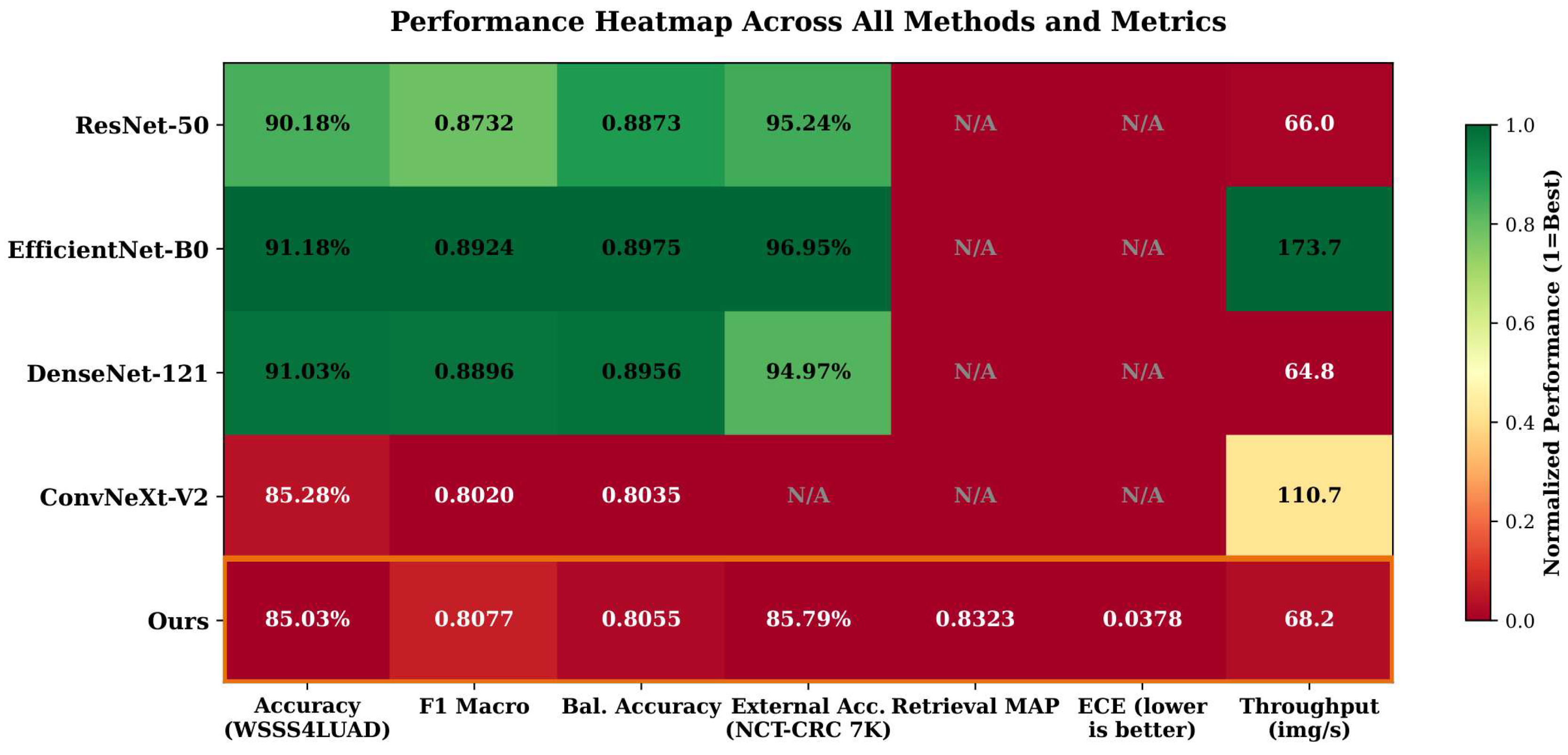
All methods and metrics performance heatmap. Green means “higher” (or “better”) performance, red means “lower” performance (for ECE, the scale is reversed–lower is better). “N/A” indicates the metric is not applicable for that method. The orange border shows the proposed system; this is the only approach that addresses all seven evaluation dimensions.
Figure 25.
All methods and metrics performance heatmap. Green means “higher” (or “better”) performance, red means “lower” performance (for ECE, the scale is reversed–lower is better). “N/A” indicates the metric is not applicable for that method. The orange border shows the proposed system; this is the only approach that addresses all seven evaluation dimensions.
Figure 26.
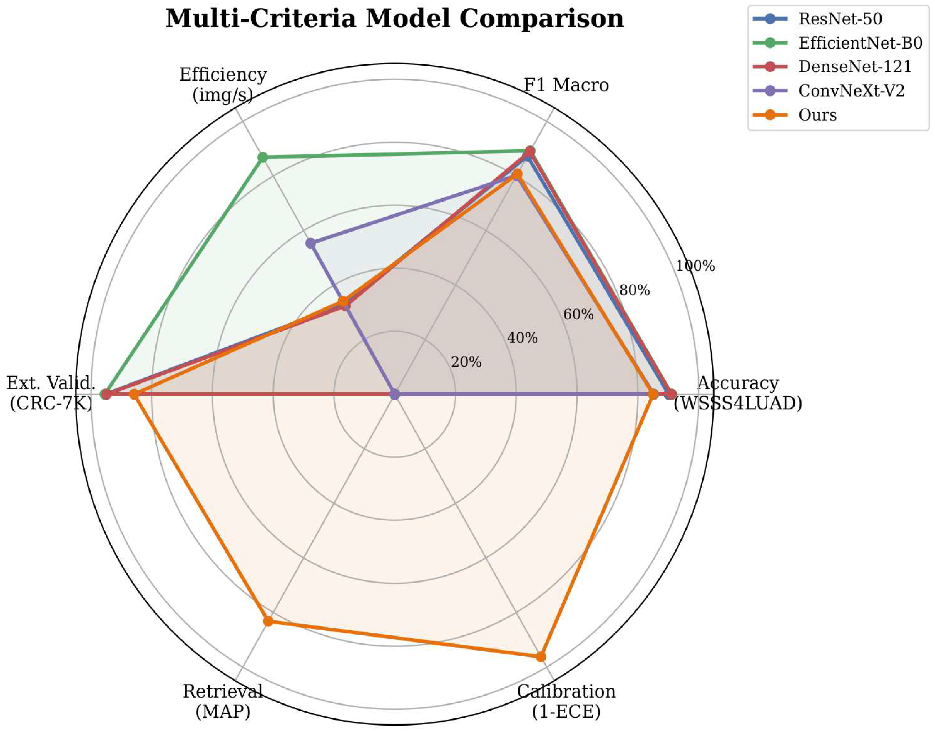
Multi-criteria radar comparison. Unlike all of the baselines, our model (orange) covers all 6 evaluation dimensions, including retrieval and calibration, which are absent in all of the baselines.
Figure 26.
Multi-criteria radar comparison. Unlike all of the baselines, our model (orange) covers all 6 evaluation dimensions, including retrieval and calibration, which are absent in all of the baselines.
Figure 27.
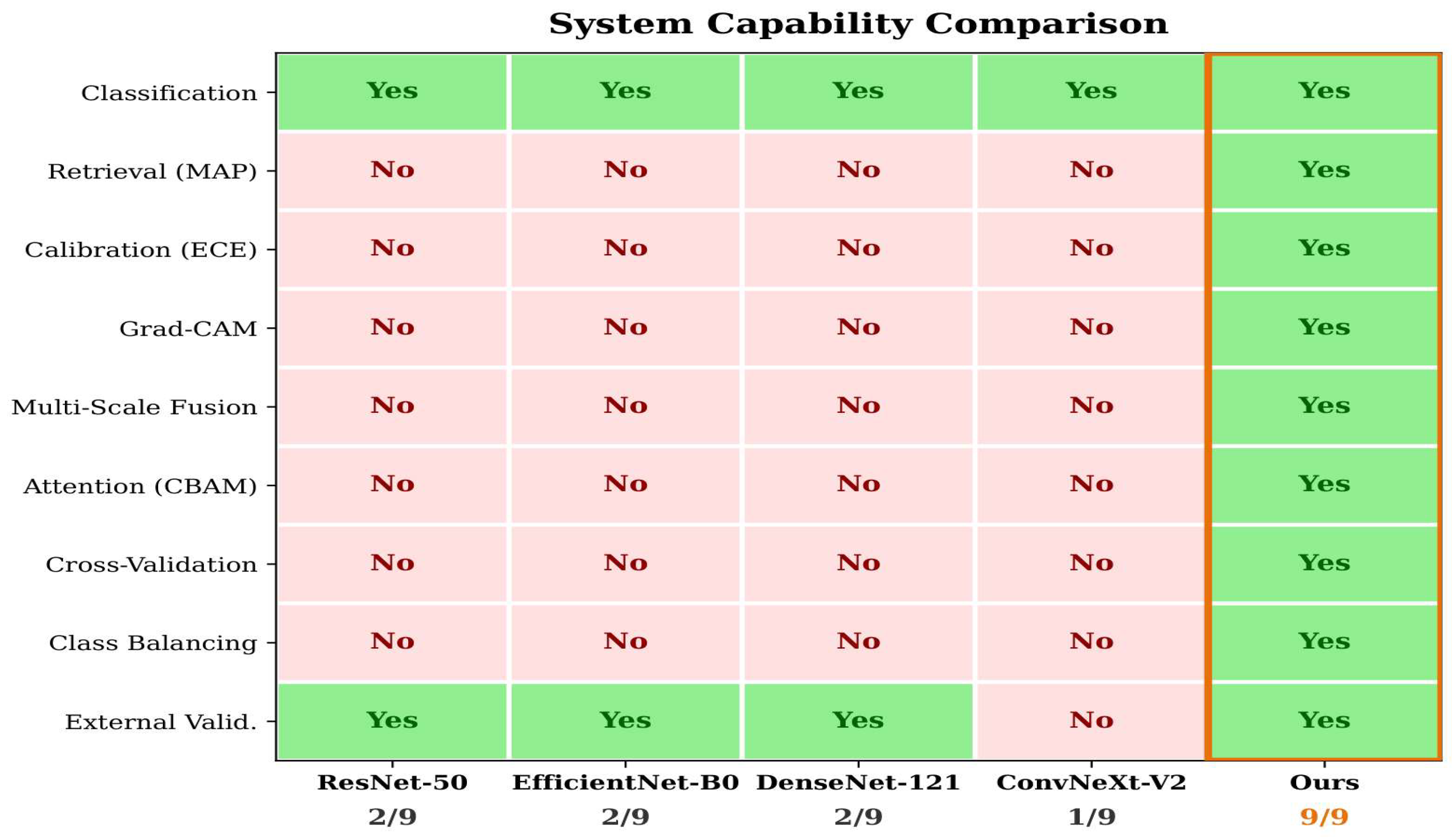
System capability matrix. The rows are the capabilities, and the cells are either “Yes” (green) or “No” (red). Our model has a 9/9 ability rating, whereas baselines have a 2/9 ability rating. The orange line outlines the proposed system.
Figure 27.
System capability matrix. The rows are the capabilities, and the cells are either “Yes” (green) or “No” (red). Our model has a 9/9 ability rating, whereas baselines have a 2/9 ability rating. The orange line outlines the proposed system.
Table 1.
Distribution of tissue classes in the WSSS4LUAD dataset.
Table 1.
Distribution of tissue classes in the WSSS4LUAD dataset.
| Class | Samples | Percentage |
|---|
| Normal | 1832 | 18.16% |
| Stroma | 1680 | 16.66% |
| Tumor | 1181 | 11.71% |
| Tumor-Stroma | 5394 | 53.48% |
| Total | 10,087 | 100% |
Table 2.
Side-by-side comparison of the datasets used in this study.
Table 2.
Side-by-side comparison of the datasets used in this study.
| Property | WSSS4LUAD | NCT-CRC-HE |
|---|
| Biological characteristics | | |
| Organ | Lung | Colon |
| Tissue type | Adenocarcinoma | Colorectal cancer |
| Staining | H&E | H&E |
| Patch size | | |
| Source WSIs | 67 | 136 [26] |
| Task properties | | |
| Classification task | 4-class | 9-class |
| Class labels | Normal, Stroma, | ADI, BACK, DEB, LYM, |
| | Tumor, Tumor-Stroma | MUC, MUS, NORM, STR, TUM |
| Class imbalance | High (53%:8%) | Moderate (14%:9%) |
| Dataset sizes | | |
| Total patches | 10,087 | 107,180 |
| Training set | 8070 (80%) | 100,000 (NCT-CRC-HE-100K) |
| Validation set | 2017 (20%) | 7180 (CRC-VAL-HE-7K) |
| Role in our study | | |
| Usage | In-domain | External validation |
| Task complexity | Lower (classes) | Higher (classes) |
| Source | Train + test | Separate held-out |
| Reference | [25] | [26] |
Table 3.
5-Fold stratified cross-validation results on WSSS4LUAD.
Table 3.
5-Fold stratified cross-validation results on WSSS4LUAD.
| Fold | Acc (%) | F1macro | Precmacro |
|---|
| Fold 1 | 83.40 | 0.7733 | 0.8134 |
| Fold 2 | 84.74 | 0.7884 | 0.8417 |
| Fold 3 | 83.39 | 0.7780 | 0.8200 |
| Fold 4 | 83.34 | 0.7731 | 0.8099 |
| Fold 5 | 81.90 | 0.7457 | 0.7949 |
| Mean ± Std | 83.35 ± 0.93 | 0.7717 ± 0.015 | 0.8160 ± 0.016 |
Table 4.
Overall classification performance on the WSSS4LUAD validation set.
Table 4.
Overall classification performance on the WSSS4LUAD validation set.
| Metric | Value |
|---|
| Accuracy | 85.03% |
| Precision (macro) | 0.8240 |
| Recall (macro) | 0.8055 |
| F1-Score (macro) | 0.8116 |
| F1-Score (weighted) | 0.8502 |
| Cohen’s Kappa () | 0.7689 |
| Weighted Kappa | 0.8841 |
| MCC | 0.7696 |
| Balanced Accuracy | 80.55% |
| Top-3 Accuracy | 99.60% |
| Log Loss | 0.4262 |
| Brier Score | 0.2226 |
| ECE | 0.0378 |
| Youden’s Index | 0.7449 |
| Diagnostic Odds Ratio | 64.25 |
Table 5.
Comparison with baseline architectures on WSSS4LUAD.
Table 5.
Comparison with baseline architectures on WSSS4LUAD.
| Model | Params (M) | Acc (%) | F1macro | Precmacro | Recmacro |
|---|
| ResNet-50 | 24.56 | 90.18 | 0.8732 | 0.8854 | 0.8634 |
| EfficientNet-B0 | 4.67 | 91.18 | 0.8924 | 0.8894 | 0.8966 |
| DenseNet-121 | 7.48 | 91.03 | 0.8896 | 0.8854 | 0.8939 |
| ConvNeXt-V2 (vanilla) | 8.82 | 85.28 | 0.8020 | 0.8435 | 0.7826 |
| Ours | 287.96 | 85.03 | 0.8077 † | 0.8343 | 0.7937 |
Table 6.
Ablation study on the WSSS4LUAD validation set.
Table 6.
Ablation study on the WSSS4LUAD validation set.
| Variant | Acc (%) | F1mac | ΔAcc | Params (M) |
|---|
| Full model (ours) | 85.03 | 0.8077 | — | 0.8077 |
| w/o CBAM | 84.09 | 0.7982 | −0.94 | 0.7982 |
| w/o Adaptive Fusion | 83.69 | 0.79^ * | −1.34 | 0.79^ * |
| w/o Spatial Branch | 83.69 | −1.34 | −1.34 | −1.34 |
| Global features only | 83.44 | 0.7825 | −1.59 | 0.7825 |
| w/o Attention Branch | 82.90 | 0.7794 | −2.13 | 0.7794 |
Table 7.
Inference efficiency comparison (GPU, BatchSize 16).
Table 7.
Inference efficiency comparison (GPU, BatchSize 16).
| Model | Params (M) | Size (MB) | GFLOPs | ms/img | img/s |
|---|
| ResNet-50 | 24.56 | 98.45 | 4.11 | 15.14 | 66.0 |
| EfficientNet-B0 | 4.67 | 18.83 | 0.40 | 5.76 | 173.7 |
| DenseNet-121 | 7.48 | 30.26 | 2.87 | 15.43 | 64.8 |
| ConvNeXt-V2 (vanilla) | 8.82 | 35.27 | 1.37 | 9.04 | 110.7 |
| Ours | 287.96 | 1151.83 | 1.78 | 14.66 | 68.2 |
Table 8.
Fair external validation: all models trained on 10.8K subsample, evaluated on CRC-VAL-HE-7K (9 Classes).
Table 8.
Fair external validation: all models trained on 10.8K subsample, evaluated on CRC-VAL-HE-7K (9 Classes).
| Model | Train Data | Acc (%) | Bal. Acc | F1mac |
|---|
| ResNet-50 | 10.8 K | 95.25 | 0.9321 | 0.9317 |
| EfficientNet-B0 | 10.8 K | 95.45 | 0.9309 | 0.9336 |
| DenseNet-121 | 10.8 K | 94.83 | 0.9230 | 0.9263 |
| Ours | 10.8 K | 85.79 | — | — |
Table 9.
Reference results: baselines trained on full 100K NCT-CRC-HE set (Ours remains at 10.8K).
Table 9.
Reference results: baselines trained on full 100K NCT-CRC-HE set (Ours remains at 10.8K).
| Model | Train Data | Acc (%) | Bal. Acc | F1mac |
|---|
| ResNet-50 | 100 K | 95.24 | 0.9348 | 0.9336 |
| EfficientNet-B0 | 100 K | 96.95 | 0.9539 | 0.9569 |
| DenseNet-121 | 100 K | 94.97 | 0.9300 | 0.9321 |
| Ours | 10.8 K | 85.79 | — | — |
Table 10.
Per-class classification performance on the WSSS4LUAD validation set.
Table 10.
Per-class classification performance on the WSSS4LUAD validation set.
| Class | Prec. | Rec. | F1 | Sens. | Spec. | PPV | NPV |
|---|
| Normal | 0.941 | 0.938 | 0.939 | 0.938 | 0.987 | 0.941 | 0.986 |
| Stroma | 0.801 | 0.872 | 0.835 | 0.872 | 0.957 | 0.801 | 0.974 |
| Tumor | 0.686 | 0.522 | 0.593 | 0.522 | 0.969 | 0.686 | 0.940 |
| T-Stroma | 0.869 | 0.890 | 0.879 | 0.890 | 0.845 | 0.869 | 0.870 |
Table 11.
Effect of class-balancing strategy on per-class performance.
Table 11.
Effect of class-balancing strategy on per-class performance.
| Strategy | Acc (%) | F1mac | Bal. Acc | Tum. R | Tum. F1 | T-S.R |
|---|
| Baseline (CE) | 85.03 | 0.8077 | 0.8055 | 0.5217 | 0.5926 | 0.8901 |
| Focal + Sampler | 76.05 | 0.7257 | 0.7588 | 0.5609 | 0.5039 | 0.7294 |
Table 12.
Architectural comparison: LGFFEM vs. ours.
Table 12.
Architectural comparison: LGFFEM vs. ours.
| Component | LGFFEM | Ours |
|---|
| Backbone | ConvNeXt V2 (Base) | ConvNeXt V2 (Base) + CBAM |
| Neck | LGFFN (BiFPN + LA/GA) | Adaptive Weighted Fusion |
| Head | GeM pooling 4 | Hybrid (Global + Spatial + Attn) |
| Descriptor dim | | 18,496 |
| Loss | Sub-center ArcFace | CE + Triplet + Label Smooth. |
| Parameters | 14.5 M | 287.96 M |
| Training data | IN-1K + PanNuke + Kimia24C | WSSS4LUAD (10,087 patches) |
| Epochs | 300 | 150 |
| Batch size | 64 | 16 |
| Optimizer | AdamW + Cosine | AdamW + Cosine + Warmup |
| Hardware | RTX 6000 ADA, 64 GB | RTX 4060, 8 GB |
| Classification | — | (85.03%) |
| Calibration | — | (ECE ) |
| Retrieval | | (MAP ) |
| Explainability | Grad-CAM (neck only) | Grad-CAM (full model) |
Table 13.
Retrieval accuracy comparison (, , ).
Table 13.
Retrieval accuracy comparison (, , ).
| Method | Dataset | Cls | Params | | | |
|---|
| DenseNet-121 | Kimia24C | 24 | 7.98 M | 95.92 | 95.51 | 91.62 |
| MA+MS-loss | Kimia24C | 24 | — | 97.89 | 97.00 | 94.95 |
| LGFFEM-A | Kimia24C | 24 | 14.5 M | 72.08 | 74.37 | 53.60 |
| LGFFEM-B | Kimia24C | 24 | 14.5 M | 77.36 | 79.28 | 61.33 |
| LGFFEM-C | Kimia24C | 24 | 14.5 M | 99.40 | 99.47 | 98.87 |
| Ours | WSSS4LUAD | 4 | 287.96 M | 85.03 † | 85.03 † | 72.03 † |
Table 14.
Content-based image retrieval performance on the WSSS4LUAD dataset.
Table 14.
Content-based image retrieval performance on the WSSS4LUAD dataset.
| P@ | R@ | NDCG@ |
|---|
| 1 | 0.8270 | 0.0520 | 0.8270 |
| 3 | 0.8169 | 0.1514 | 0.8810 |
| 5 | 0.8127 | 0.2495 | 0.8891 |
| 10 | 0.8065 | 0.4953 | 0.8948 |