Risk-Aware Cost-Constrained Scheduling for Resource- Constrained Dynamic Heterogeneous Redundancy Systems

Abstract

Resource-constrained dynamic heterogeneous redundancy (DHR) systems use executor diversity and runtime reconfiguration to reduce stable attack surfaces. However, effective scheduling cannot rely only on heterogeneity or movement frequency, because repeated exposure, shared vulnerability sources, service disturbance, and switching overhead jointly shape executor-subset selection. This paper proposes RACS, a risk-aware cost-constrained scheduling method for resource-constrained DHR systems. RACS evaluates candidate subsets by jointly considering heterogeneity, historical confidence, readiness, common-vulnerability risk, exposure memory, and switching cost. We evaluate RACS using a controlled simulation protocol covering multiple scheduling principles and attacker behaviors, including common-vulnerability pressure, burst-adaptive exploitation, and adaptive target selection based on observed scheduling patterns. The results show that RACS does not optimize a single metric in isolation, but maintains a consistent security–cost trade-off. It reduces common-vulnerability risk and switching cost in common-vulnerability settings, reduces burst-triggering high-risk states under adaptive pressure, and maintains competitive risk–cost behavior when attackers adapt to historical scheduling behavior. Robustness and scalability analyses clarify the effects of vulnerability-family estimation errors, parameter choices, and executor-pool size. These findings provide controlled simulation evidence for joint risk–cost modeling in DHR executor-subset scheduling, while testbed validation remains future work.

1. Introduction

Dynamic heterogeneous redundancy (DHR) is an important technical route in cyberspace mimic defense. Its basic idea is to improve service resilience through heterogeneous executors, redundant execution, adjudication, and dynamic scheduling. Similar to earlier ideas such as design diversity and N-version programming, DHR aims to use implementation diversity and runtime uncertainty to weaken the effects of common-mode failures and stable attack paths [1,2]. It is also closely related to the mimic-defense framework proposed for designed-in cybersecurity defense [3]. The core security rationale is that an attacker should not be able to rely on a fixed execution environment to continuously compromise a target system.

In DHR systems, the scheduling mechanism directly determines which executors are selected to participate in service execution at each round. Therefore, scheduling affects not only resource usage, but also the dynamic security state of the system. Existing scheduling designs usually emphasize executor heterogeneity, historical reliability, or scheduling variation frequency [4,5,6,7,8], but these signals alone cannot sufficiently characterize the security–cost trade-off in resource-constrained settings. Specifically, high historical confidence does not necessarily imply low future risk. Even if an executor has behaved reliably in the past, frequent selection may allow attackers to continuously observe and learn its behavioral patterns and interaction characteristics. This repeated visibility can cause exposure accumulation. Feature-level heterogeneity also does not necessarily imply vulnerability-family independence. Executors may differ in implementation, configuration, or runtime environment, but they may still share similar underlying components, dependencies, or vulnerability families, creating common-vulnerability overlap that can lead to correlated compromise [1,2,9]. In addition, dynamic movement itself incurs operational cost. Frequent executor switching can reduce stable exposure, but it may also increase switching overhead and service disturbance, weakening the practical cost-effectiveness of the defense strategy [10,11,12,13,14].

These issues indicate that DHR executor-subset scheduling should not be simplified as heterogeneity maximization, historical-confidence prioritization, or movement-frequency control. A more appropriate modeling view is to treat it as a subset-level risk–cost decision problem: the scheduler needs to jointly consider functional heterogeneity, historical behavior, common-vulnerability risk, exposure memory, and switching cost of candidate executor subsets, and then balance security benefit against operational cost [8,14,15]. From this view, historical reliability and repeated exposure, feature heterogeneity and vulnerability independence, and scheduling movement and security improvement should be treated as different types of scheduling signals rather than being simply substituted for or merged with one another.

Existing DHR and moving target defense scheduling studies have explored this problem from the perspectives of randomization, heterogeneity utilization, historical confidence, resource constraints, and cost control. Moving target defense surveys and early MTD studies provide the broader proactive-defense context and discuss adaptation, effectiveness, affordability, optimization, randomization, and game-theoretic strategy selection [10,11,12,13,16,17]. Entropy-weighted resource scheduling has been studied for CRCC-DHR under limited heterogeneous resources and memorization-based attacks [8]. Heterogeneity and historical confidence have been combined for mimic-defense executor scheduling [4]. Sliding-window, seed-scheduling, and service-function-chain scheduling studies consider feedback, timing, internal resource constraints, load, and security–cost balance [5,6,15]. Dynamic scheduling has also been considered in volunteer-computing mimic-defense architectures [7].

These studies provide important foundations for executor scheduling. However, their focus is usually placed on a single or local scheduling principle. For example, randomization and rotation strategies mainly rely on uncertainty introduced by movement; heterogeneity-driven methods emphasize executor differences; confidence-driven methods tend to prefer historically reliable executors; and resource- or entropy-weighted methods focus more on resource-use distribution. For resource-constrained DHR systems, relying on only one type of signal may lead to partial scheduling behavior: high-confidence executors may be repeatedly exposed, highly heterogeneous subsets may still contain common-vulnerability risk, and high-frequency movement may introduce excessive operational cost. Therefore, it is necessary to jointly characterize repeated exposure, common-vulnerability risk, and switching cost in subset-level scoring.

This paper proposes Risk-Aware Cost-Constrained Scheduling (RACS) for executor-subset selection in DHR systems. RACS treats each candidate executor subset as the scoring object and jointly models executor heterogeneity, historical confidence, common-vulnerability risk, exposure memory, and switching cost within a unified scoring rule. The core idea is to incorporate common-vulnerability risk, repeated visibility, and the operational cost caused by defensive movement into scheduling decisions, rather than relying only on heterogeneity, historical confidence, or movement frequency. This paper examines whether a risk-aware subset-level scoring method can produce consistent security–cost behavior compared with randomized, confidence-based, entropy-weighted, budget-constrained, cost-aware MDP-based, model-predictive, Pareto-based, and game-theoretic scheduling under controlled attacker stress settings.

The main contributions of this paper are summarized as follows:

• We propose RACS, a risk-aware and cost-constrained scheduling method for executor-subset selection in resource-constrained DHR systems. RACS treats candidate executor subsets as scoring objects and incorporates executor heterogeneity, historical confidence, common-vulnerability risk, exposure memory, and switching cost into a unified scoring rule, avoiding the simplification of scheduling decisions into single-indicator optimization.
• We explicitly distinguish three easily conflated scheduling signals: historical reliability and repeated exposure, feature heterogeneity and vulnerability independence, and movement frequency and actual security improvement. This modeling design allows the scheduler to jointly consider common-vulnerability risk, repeated exposure, switching cost, and service disturbance.
• We design a reproducible controlled risk–cost stress-testing protocol that covers common-vulnerability, burst-adaptive, and best-response adaptive attacker settings. The experiments compare RACS with representative scheduling principles and further analyze its ablation behavior, parameter sensitivity, vulnerability-estimation robustness, and scalability boundary.

2. Related Work

2.1. Cyber Mimic Defense and Dynamic Heterogeneous Redundancy

Cyber mimic defense and dynamic heterogeneous redundancy (DHR) provide the architectural background of this study. Their common rationale is to reduce the value of static attack knowledge through executor diversity, redundant execution, arbitration, and dynamic transformation [3]. This line of work is closely related to design-diverse redundant software and N-version programming, where common-mode failures, variant independence, and diversity effects have long been central concerns [1,2,9]. Intrusion-tolerance research also provides a related dependability-security perspective by studying how systems can continue to provide services in the presence of compromised components [18]. In the context of cyberspace mimic defense, DHR further emphasizes heterogeneous executors and dynamic scheduling as mechanisms for weakening stable attack paths.

In DHR systems, architectural executor diversity is only one prerequisite for security benefits, and runtime scheduling also affects the risk state of the system. Even when an executor pool is highly heterogeneous, a scheduler may repeatedly expose a small number of executors or executor combinations, giving attackers more stable observation targets. Conversely, overly frequent executor switching may reduce stable exposure, but it can also introduce additional operational cost and service disturbance. Therefore, DHR executor selection is not only a problem of using diversity but also a runtime trade-off among repeated exposure, common-vulnerability risk, and switching overhead.

2.2. Executor Scheduling in DHR Systems

Executor scheduling in DHR has moved beyond simple random or periodic replacement. Guo et al. studied scheduling sequence control using a sliding-window mechanism and considered internal resource constraints and external attack situations [5]. Chen et al. investigated seed scheduling for cyberspace mimic defense [6]. Li et al. proposed threshold and multi-level-queue scheduling for volunteer-computing cyber mimic defense [7]. Zhang et al. combined heterogeneity and historical confidence for mimic-defense executor scheduling, which is closely related to confidence-based executor selection [4]. These studies show that DHR scheduling has already incorporated timing control, resource constraints, feedback, historical reliability, and operating efficiency.

Existing scheduling studies provide an important basis for executor selection, but executor exposure, historical confidence, and heterogeneity are not the same type of state. A confidence-oriented scheduler usually tends to select executors that have behaved correctly in previous rounds. However, an executor may remain historically reliable while becoming a stable attack-observation surface due to repeated selection. In this case, high historical confidence does not necessarily imply low future risk.

Similarly, a highly heterogeneous executor subset does not necessarily imply vulnerability-family independence. If different executors share the same vulnerability family or depend on similar underlying components, the scheduler may still select a subset with high common-vulnerability risk, which can lead to correlated compromise. In addition, if a scheduler mainly relies on frequent switching to reduce exposure, it may introduce additional operational cost and service disturbance. Therefore, executor-subset scheduling should not only consider heterogeneity and historical confidence, but also characterize the effects of exposure accumulation, vulnerability-family overlap, and switching cost on scheduling behavior.

2.3. Cost-Aware and Uncertainty-Aware Dynamic Defense

Cost and uncertainty are also important issues in DHR and moving target defense. Wu et al. proposed an entropy-weighted resource scheduling method for CRCC-DHR under limited heterogeneous resources and memorization-based attacks [8]. This work is closely related to this study because it has already considered resource constraints and attacker memory in DHR scheduling. Compared with this type of method, the present study focuses more on subset-level risk–cost scoring, where repeated executor exposure, common-vulnerability risk, and switching cost are evaluated within the same candidate-subset selection rule. Therefore, an entropy-style scheduler is included as a related baseline in the experiments.

Beyond resource-constrained scheduling, recent DHR and mimic-defense studies have extended dynamic defense mechanisms from several adjacent perspectives. Differentially private DHR decision methods focus on privacy-preserving perturbation and decision strategies [19]. Output-difference feedback and system-benefit control methods study the trade-off among adjudication feedback, security benefit, and system overhead [20]. AI-enhanced mimic-defense methods and reinforcement-learning-based scheduling methods learn scheduling strategies through training objectives, reward definitions, and resource-utilization criteria [21,22]. Service-function-chain scheduling further considers abnormal-executor feedback, heterogeneity, system load, and security–cost balance [15]. These studies enrich the technical paths of DHR scheduling and dynamic defense, but their main focus is usually on privacy protection, adjudication feedback, learning-based decision making, service-chain management, or system-level control, rather than on constructing an explicit risk–cost scoring rule for DHR executor-subset selection.

The broader moving target defense literature also shows that dynamic movement does not automatically bring security benefits. Studies on attack-surface measurement, network and IP randomization, cyber-physical randomization, deception-based MTD, game-theoretic defense, and MDP-based strategy selection show that movement can increase attacker uncertainty, but it may also introduce reconfiguration cost, incomplete coverage, or predictable movement patterns [14,23,24,25,26,27,28,29,30,31,32]. These studies usually operate at the network, service-placement, system-configuration, or strategy-selection level. In contrast, this paper focuses on the more specific level of DHR executor-subset selection and studies whether risk–cost scoring can lead to more favorable security–cost behavior when executor historical reliability, runtime exposure, common-vulnerability risk, and switching cost coexist.

Decision-theoretic and game-theoretic MTD studies are also relevant to the scheduling problem considered here. Empirical game-theoretic methods have been used to generate MTD strategies in web-application settings, and spatial-temporal MTD has been formulated as a Markov Stackelberg game in which the defender considers configuration sequences and switching timing under migration costs [33,34]. More recent work further studies adversarial MTD decision making through multi-agent Markov games and reinforcement learning [35]. These studies motivate the inclusion of cost-aware MDP-style and game-theoretic baselines in this paper, but they generally operate at the MTD strategy-selection or configuration-management level rather than at the DHR executor-subset scoring level.

3. System and Threat Model

3.1. Resource-Constrained DHR System

This paper considers a resource-constrained dynamic heterogeneous redundancy system. The system contains a pool of n functionally equivalent executors $E=\{e_1,\dots ,e_n\}$. Each executor can provide the target service, but executors differ in implementation features, vulnerability-family membership, service latency, throughput capacity, historical confidence, exposure memory, switching cost, and cooldown state. At scheduling round t, the scheduler selects a fixed-size subset $S_t\subset E$ for redundant execution. The base experiments use $k=3$, which supports majority-style arbitration while keeping candidate-subset enumeration computationally tractable.

The service request is processed by all executors in $S_t$. If the attacker compromises a majority of the selected subset in the same round, the round is recorded as an attack success; otherwise, it is recorded as a defense success. When $k=3$, attack success means that at least two selected executors are compromised in that round. This abstraction preserves the basic redundant-execution and majority-arbitration rationale of DHR systems without binding the model to a specific production voter, output-comparison strategy, or recovery mechanism.

The resource-constrained aspect appears in two places. First, the system cannot activate all executors in every round, so the scheduler must select a subset under limited resources. Second, changing the selected executor subset incurs operational cost, including state transfer, warm-up, container replacement, service migration, reconfiguration, or other switching-related overhead. The simulator therefore treats security outcomes and operational costs as jointly observed quantities rather than optimizing attack success rate alone.

3.2. Executor Pool and Adjudication Model

Executor $e_i$ is represented at round t by the state tuple

$$x_i\left(t\right)=\{h_i,F_i,C_i\left(t\right),M_i\left(t\right),L_i,Q_i,{\kappa }_i,R_i\left(t\right)\},$$

(1)

where $h_i$ is the heterogeneity feature vector, $F_i$ is the vulnerability-family set, $C_i\left(t\right)$ is historical confidence, $M_i\left(t\right)$ is exposure memory, $L_i$ is service latency, $Q_i$ is throughput capacity, ${\kappa }_i$ is the executor-level switching-cost factor, and $R_i\left(t\right)$ denotes cooldown readiness.

These variables define the controlled experimental state used by the simulator. The model does not assume that all variables are fully, accurately, and immediately observable in a deployed system. Instead, the state representation is used to isolate and measure the effects of different scheduling mechanisms, so that heterogeneity, confidence, exposure, common-vulnerability risk, and switching cost can be recorded and compared within the same experimental environment.

Adjudication is modeled at the round level. If the attacker compromises fewer than a majority of selected executors, the service round is considered defended. If the attacker compromises a majority, the round is counted as an attack success and contributes to metrics such as mean time to compromise and continuous safe rounds. Application-specific output comparison, voter design, fault recovery, and state-cleaning mechanisms are outside the scope of this scheduling model.

3.3. Executor State Update

Exposure memory evolves as

$$M_i(t+1)=\rho M_i\left(t\right)+\alpha I(e_i\in S_t)+\beta A_i\left(t\right),$$

(2)

where $M_i\left(t\right)$ is the exposure memory of executor $e_i$ at round t, $I(e_i\in S_t)$ indicates whether the executor is selected, $A_i\left(t\right)$ denotes attack observation or abnormal behavior, $\rho$ is the exposure decay factor, and $\alpha$ and $\beta$ control the gains from routine service exposure and attack-related exposure, respectively.

Exposure memory is a defender-side repeated-visibility proxy. It captures the visibility accumulated by an executor through repeated service participation or attack-related observation. When an executor is not repeatedly selected or attacked, its exposure value decays over time. The term $\alpha I(e_i\in S_t)$ represents visibility introduced by routine service traffic, while $\beta A_i\left(t\right)$ represents additional visibility associated with attack observation or abnormal behavior. In the base configuration, the attack-related exposure gain is larger than the routine selection gain. This reflects the assumption that attack observation has stronger influence on future scheduling risk.

Historical confidence $C_i\left(t\right)$ is updated separately according to service outcomes, compromise outcomes, and recovery outcomes. It represents the scheduler’s estimate of executor reliability or trustworthiness based on observed behavior. Exposure memory $M_i\left(t\right)$, in contrast, is not a reliability estimate; it is a state variable associated with repeated selection and attack visibility. Thus, an executor may have both high historical confidence and high exposure: it may continue to produce correct outputs while also being visible to the attacker for many rounds. This distinction is an important basis for the scheduling score defined later.

3.4. Attacker Models

The simulator considers three main attacker settings: the common-vulnerability attacker, the burst-adaptive attacker, and the best-response adaptive attacker. They are designed to stress different scheduling-induced risks under the same DHR abstraction. In all settings, a round is counted as an attack success if a majority of the selected executor subset is compromised in that round. For the base setting with $k=3$, this means that at least two of the three selected executors are compromised.

The common-vulnerability attacker stresses correlated compromise caused by shared vulnerability families. It becomes more effective when the selected subset contains executors with overlapping vulnerability-family memberships. This setting examines whether a scheduler can avoid executor combinations that appear diverse at the feature level but still share common vulnerability sources.

The burst-adaptive attacker stresses the joint effect of repeated exposure and common-vulnerability risk. When the selected subset has both high mean exposure and high common-vulnerability risk, the attacker enters a short enhanced attack state. At the subset level, the compromise pressure is modeled as

$$p_{\mathrm{comp}}\left(S_t\right)=p_0+{\gamma }_e\overline{M}\left(S_t\right)+{\gamma }_{v}V\left(S_t\right)+{\gamma }_{ev}\overline{M}\left(S_t\right)V\left(S_t\right),$$

(3)

where $\overline{M}\left(S_t\right)$ is the mean exposure memory of the selected subset and $V\left(S_t\right)$ is the common-vulnerability risk. The interaction term $\overline{M}\left(S_t\right)V\left(S_t\right)$ captures the case where repeated visibility and common-vulnerability risk jointly increase attack pressure. This setting tests whether a scheduler can avoid states with both high exposure and high common-vulnerability risk.

The best-response adaptive attacker represents an informed adaptive setting. It observes historical scheduling behavior and maintains an attacker-side observation state $O_i\left(t\right)$ for each executor:

$$O_i(t+1)={\rho }_o{O}_i\left(t\right)+{\alpha }_o\mathbb{I}(e_i\in S_t),$$

(4)

where ${\rho }_o$ is the observation-memory decay factor and ${\alpha }_o$ is the observation gain when executor $e_i$ is selected. The attacker-side observation state $O_i\left(t\right)$ is different from the defender-side exposure memory $M_i\left(t\right)$: $O_i\left(t\right)$ represents the attacker’s inferred target interest from observed scheduling history, whereas $M_i\left(t\right)$ is maintained by the scheduler as a repeated-visibility proxy.

In each round, the best-response adaptive attacker assigns higher compromise pressure to selected executors that are frequently observed, have higher exposure, share more vulnerability families with the current subset, or have lower historical confidence. The attacker does not know the scheduler’s future random choices or internal random seed, but it can exploit scheduling tendencies that have already been observed. This setting evaluates whether RACS maintains interpretable risk–cost behavior when the attacker adapts to historical scheduling patterns.

4. Risk-Aware Cost-Constrained Scheduling

4.1. Design Motivation

DHR scheduling needs to handle security risk and operational cost together. Repeatedly selecting the same executor may create stable exposure even when that executor remains historically reliable. Selecting executors only for diversity may ignore common-vulnerability risk caused by shared vulnerability families. Frequent executor switching may reduce stable exposure, but it can also introduce additional operational overhead and service disturbance.

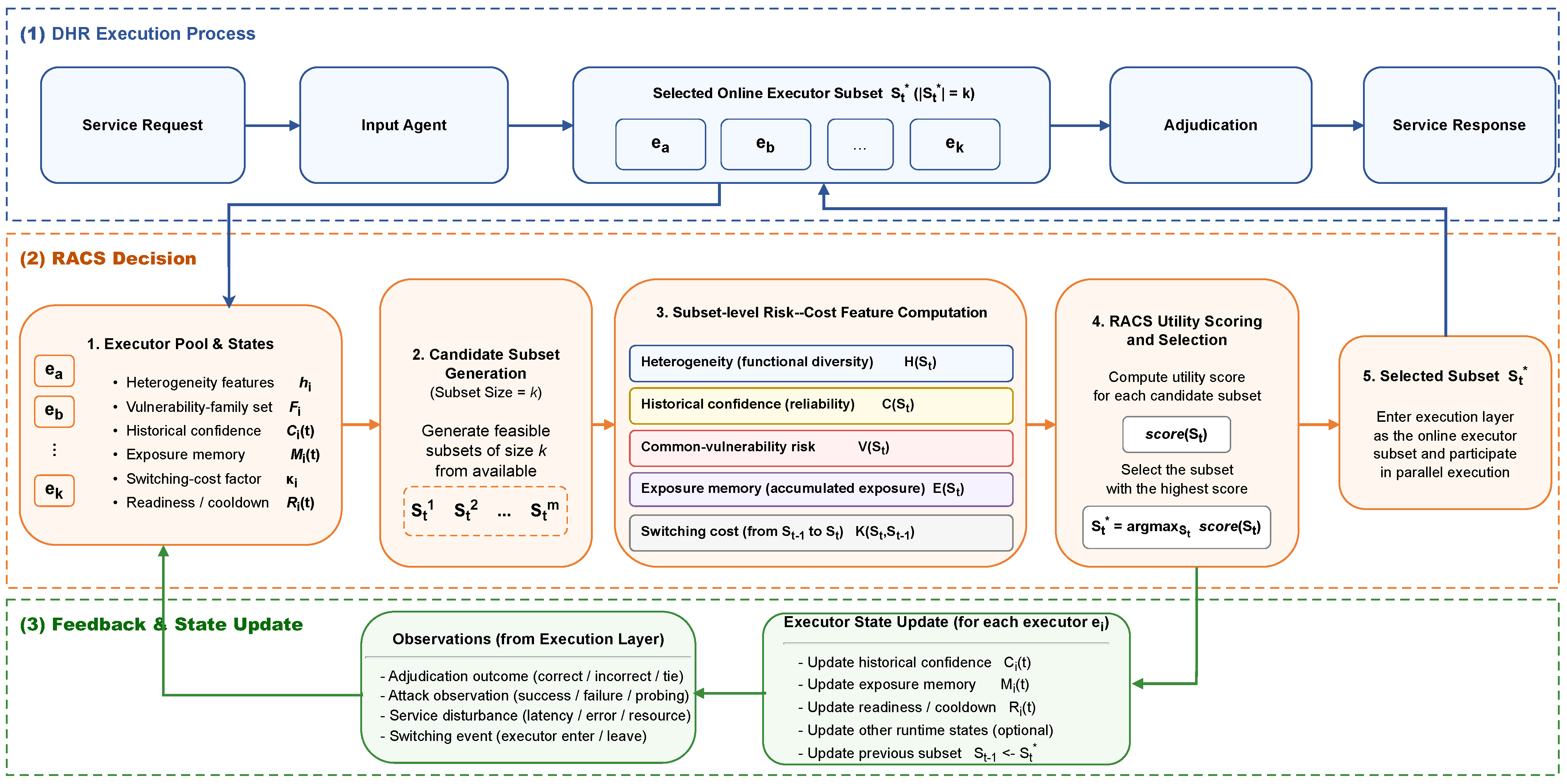
Figure 1 provides a workflow overview of the proposed RACS scheduler within a resource-constrained DHR system. It shows how service requests enter the DHR execution layer, how candidate executor subsets are generated and scored, and how adjudication outcomes, attack observations, service disturbance, and switching events are fed back to update executor states. The figure is used as a roadmap for the scheduling loop, while the following subsections define the subset-level features and scoring rule in detail.

Based on this consideration, this paper proposes RACS, a risk-aware and cost-constrained heuristic scheduler for DHR executor-subset selection. Here, risk-aware means that the scheduler explicitly considers repeated exposure and common-vulnerability risk; cost-constrained means that switching cost and service impact are evaluated together with security outcomes. RACS treats heterogeneity, historical confidence, common-vulnerability risk, exposure memory, and switching cost as the main scheduling signals, while cooldown readiness is retained as an auxiliary readiness state in the simulator.

RACS is designed as an interpretable subset-level scoring rule whose components correspond to observable mechanisms and can be individually removed in ablation studies. This design makes it possible to examine how different risk–cost factors influence scheduling behavior.

4.2. Exposure Is Not Historical Confidence

Historical confidence and exposure memory are explicitly separated in RACS. Historical confidence is updated according to an executor’s past service reliability, compromise outcomes, and recovery outcomes. It answers the question of which executors appear reliable based on historical behavior. Exposure memory answers a different question: which executors have become more visible due to repeated selection or attack observation?

This distinction affects scheduling behavior. A purely confidence-driven scheduler may repeatedly choose the same reliable executors, concentrating attacker observation and increasing memorization opportunities. A purely exposure-avoidant scheduler may rotate too aggressively and ignore reliability or operational cost. RACS uses both confidence and exposure memory, so that historical reliability remains useful while repeated visibility is penalized.

4.3. Executor-Subset Features

At each round, RACS reads the executor state tuple and computes subset-level features for each candidate subset. Heterogeneity $H\left(S_t\right)$ is computed from pairwise distances among the feature vectors of selected executors. Mean confidence $C\left(S_t\right)$ is the average historical confidence of selected executors. Cooldown readiness $R\left(S_t\right)$ indicates whether the selected executors are available and suitable for scheduling. Common-vulnerability risk $V\left(S_t\right)$ is computed from vulnerability-family overlap. Mean exposure $E\left(S_t\right)$ is the average exposure memory of selected executors. Switching cost $K(S_t,S_{t-1})$ is computed from the changes between the current subset and the previous subset.

The weights used in the experiments are fixed in the configuration files to ensure reproducibility. Different operational environments may have different latency, throughput, switching-overhead, and risk scales, so practical deployment would require system-specific weight calibration.

4.4. Exposure Memory and Cooldown Update

The exposure update is given by Equation (2). When an executor is selected, its exposure value increases due to service participation. When an executor is attacked or exhibits abnormal behavior, its exposure value further increases. The decay factor $\rho$ controls how quickly historical exposure loses influence. When $\rho$ is close to one, exposure memory is more persistent; when $\rho$ is smaller, old exposure has less influence on future scheduling.

The selection gain $\alpha$ captures the visibility introduced by routine service requests, while the attack gain $\beta$ captures additional visibility associated with attack observation or abnormal behavior. The base configuration sets $\beta >\alpha$. This setting gives attack-related exposure stronger influence on future scheduling risk.

Cooldown state is modeled as an auxiliary readiness variable after attack-related events, representing possible short-term recovery or cautious-use conditions. The experiments focus on the main scoring factors: common-vulnerability risk, exposure memory, and switching-cost control.

4.5. Common-Vulnerability Risk

Common-vulnerability risk characterizes vulnerability-family overlap among selected executors. Let $F_i$ denote the vulnerability-family set of executor $e_i$. For a candidate subset $S_t$, RACS computes pairwise vulnerability-family overlap among the selected executors and averages it over all executor pairs:

$$V\left(S_t\right)={\displaystyle \frac{2}{|S_t\left|\right(|S_t|-1)}}\sum _{i<j,e_i,e_j\in S_t}{\displaystyle \frac{|F_i\cap F_j|}{|F_i\cup F_j|+ϵ}},$$

(5)

where $ϵ$ avoids division by zero. A larger $V\left(S_t\right)$ indicates greater vulnerability-family overlap among selected executors and therefore higher common-vulnerability risk, which can increase the likelihood of correlated compromise.

Common-vulnerability risk is distinct from heterogeneity. Two executors may be far apart in feature space but still share a vulnerability family. Conversely, two executors may be similar in some implementation features while not sharing the modeled vulnerability family. Therefore, RACS retains both a heterogeneity reward and a common-vulnerability penalty, encouraging diverse executor subsets while avoiding subsets with high common-vulnerability risk.

4.6. Cost-Constrained Scheduling Utility

For a candidate subset $S_t$, RACS computes

$$\begin{array}{cc}\hfill score\left(S_t\right)=& {\lambda }_{h}H\left(S_t\right)+{\lambda }_{c}C\left(S_t\right)+{\lambda }_{r}R\left(S_t\right)\hfill \\ \hfill & -{\lambda }_{v}V\left(S_t\right)-{\lambda }_{e}E\left(S_t\right)-{\lambda }_{s}K(S_t,S_{t-1}),\hfill \end{array}$$

(6)

where H is heterogeneity, C is mean confidence, R is cooldown readiness, V is common-vulnerability risk, E is mean exposure, and K is switching cost relative to the previously selected subset. The scheduler enumerates all feasible candidate subsets and selects the subset with the highest score.

The positive terms reward desirable subset properties, including executor diversity, historical reliability, and short-term readiness. The negative terms penalize undesirable risk and cost, including vulnerability-family overlap, repeated exposure, and switching overhead. The switching term prevents the scheduler from reducing risk indicators through unrestricted movement without accounting for operational overhead. In this way, RACS places security risk, executor state, and operational cost in the same candidate-subset selection rule.

4.7. Theoretical Interpretation

RACS can be formulated as a penalty-based scalarized scoring rule for a constrained executor-subset selection problem. At each scheduling round, the scheduler selects a feasible executor subset with high heterogeneity, historical confidence, and readiness, while controlling common-vulnerability risk, accumulated exposure, and switching cost. This objective can be written as

$$\begin{array}{cc}\hfill \underset{S_t\subseteq E,\left|S_t\right|=k}{max}& U\left(S_t\right)=H\left(S_t\right)+C\left(S_t\right)+R\left(S_t\right),\hfill \\ \hfill \mathrm{s}.\mathrm{t}.& V\left(S_t\right)\le b_v,E\left(S_t\right)\le b_e,K(S_t,S_{t-1})\le b_k.\hfill \end{array}$$

(7)

Here, $b_v$, $b_e$, and $b_k$ denote the upper bounds on common-vulnerability risk, selected exposure, and switching cost, respectively. RACS incorporates these risk and cost factors into a penalty-based score and ranks candidate subsets at each scheduling round:

$$\begin{array}{cc}\hfill score\left(S_t\right)=& {\lambda }_{h}H\left(S_t\right)+{\lambda }_{c}C\left(S_t\right)+{\lambda }_{r}R\left(S_t\right)\hfill \\ \hfill & -{\lambda }_{v}V\left(S_t\right)-{\lambda }_{e}E\left(S_t\right)-{\lambda }_{s}K(S_t,S_{t-1}).\hfill \end{array}$$

(8)

In this score, H, C, and R are reward terms corresponding to heterogeneity, historical confidence, and readiness, respectively. The terms V, E, and K are penalty terms corresponding to common-vulnerability risk, accumulated exposure, and switching cost. The following analysis assumes that all score terms are finite scalars under the current executor pool and experimental configuration, and that all RACS weights are nonnegative:

$${\lambda }_h,{\lambda }_c,{\lambda }_r,{\lambda }_v,{\lambda }_e,{\lambda }_s\ge 0.$$

(9)

Proposition 1 

(Bounded exposure memory). If $0\le \rho <1$, $I(e_i\in S_t)\in [0,1]$, and $A_i\left(t\right)\in [0,1]$, then the exposure memory updated by

$$M_i(t+1)=\rho M_i\left(t\right)+\alpha I(e_i\in S_t)+\beta A_i\left(t\right)$$

(10)

satisfies

$$M_i\left(t\right)\le {\rho }^t{M}_i\left(0\right)+{\displaystyle \frac{\alpha +\beta }{1-\rho }}.$$

(11)

Proof. 

By unrolling the exposure-memory recurrence and using $I(e_i\in S_{\tau })\le 1$ and $A_i\left(\tau \right)\le 1$, we obtain

$$\begin{array}{cc}\hfill M_i\left(t\right)& ={\rho }^t{M}_i\left(0\right)+{\displaystyle \sum _{\tau =0}^{t-1}}{\rho }^{t-1-\tau }\left(\alpha I(e_i\in S_{\tau })+\beta A_i\left(\tau \right)\right)\hfill \\ \hfill & \le {\rho }^t{M}_i\left(0\right)+(\alpha +\beta ){\displaystyle \sum _{\tau =0}^{t-1}}{\rho }^{t-1-\tau }\hfill \\ \hfill & ={\rho }^t{M}_i\left(0\right)+(\alpha +\beta ){\displaystyle \frac{1-{\rho }^t}{1-\rho }}\hfill \\ \hfill & \le {\rho }^t{M}_i\left(0\right)+{\displaystyle \frac{\alpha +\beta }{1-\rho }}.\hfill \end{array}$$

(12)

Thus, exposure memory is a bounded exponentially decayed state. Since $E\left(S\right)$ is obtained by aggregating the exposure states of a finite number of selected executors, $E\left(S\right)$ is also finite under the given configuration.    □

Proposition 2 

(Monotonicity and switching-cost preference of the RACS score). Under nonnegative weights, when all other terms are fixed, increasing $H\left(S\right)$, $C\left(S\right)$, or $R\left(S\right)$ cannot decrease the RACS score. Increasing $V\left(S\right)$, $E\left(S\right)$, or $K(S,S_{t-1})$ cannot increase the RACS score.

Proof. 

The gradient of the RACS score with respect to $(H,C,R,V,E,K)$ is

$$\nabla score=({\lambda }_h,{\lambda }_c,{\lambda }_r,-{\lambda }_v,-{\lambda }_e,-{\lambda }_s).$$

(13)

Since all weights are nonnegative, $score\left(S\right)$ is nondecreasing in H, C, and R, and nonincreasing in V, E, and K. Therefore, increasing a reward term cannot decrease the score, and increasing a penalty term cannot increase the score.

Furthermore, let $U_0\left(S\right)$ collect all score terms except switching cost:

$$U_0\left(S\right)={\lambda }_{h}H\left(S\right)+{\lambda }_{c}C\left(S\right)+{\lambda }_{r}R\left(S\right)-{\lambda }_{v}V\left(S\right)-{\lambda }_{e}E\left(S\right).$$

(14)

Then

$$score\left(S\right)=U_0\left(S\right)-{\lambda }_{s}K(S,S_{t-1}).$$

(15)

For two candidate subsets $S_a$ and $S_b$, suppose that $U_0\left(S_a\right)=U_0\left(S_b\right)$ and

$$K(S_a,S_{t-1})<K(S_b,S_{t-1}).$$

(16)

Then $score\left(S_a\right)>score\left(S_b\right)$ when ${\lambda }_s>0$. Let $K_a=K(S_a,S_{t-1})$ and $K_b=K(S_b,S_{t-1})$. Since $U_0\left(S_a\right)=U_0\left(S_b\right)$ and $K_a<K_b$,

$$score\left(S_a\right)-score\left(S_b\right)=-{\lambda }_s(K_a-K_b)>0,{\lambda }_s>0.$$

(17)

In addition,

$${\displaystyle \frac{\partial (score\left(S_a\right)-score\left(S_b\right))}{\partial {\lambda }_s}}=K_b-K_a>0.$$

(18)

Thus, under identical non-switching utility, the lower-switching-cost subset receives a higher score, and increasing ${\lambda }_s$ increases its relative score advantage over the higher-switching-cost subset.    □

Proposition 3 

(Pareto consistency of the RACS score). Let $S_a,S_b\in {\mathcal{F}}_t$ be two feasible candidate subsets, where

$${\mathcal{F}}_t=\{S\subseteq E:|S|=k,S\mathit{is}\mathit{feasible}\mathit{at}\mathit{round}t\}.$$

(19)

Define the reward vector and the risk–cost vector as

$$r\left(S\right)=(H\left(S\right),C\left(S\right),R\left(S\right)),p\left(S\right)=(V\left(S\right),E\left(S\right),K(S,S_{t-1})).$$

(20)

If $r\left(S_a\right)⪰r\left(S_b\right)$ and $p\left(S_a\right)⪯p\left(S_b\right)$, with at least one strict inequality associated with a positive corresponding weight, then

$$score\left(S_a\right)>score\left(S_b\right).$$

(21)

Proof. 

Let

$${\lambda }^{+}=({\lambda }_h,{\lambda }_c,{\lambda }_r),{\lambda }^{-}=({\lambda }_v,{\lambda }_e,{\lambda }_s).$$

(22)

The score difference between the two candidate subsets can be written as

$$score\left(S_a\right)-score\left(S_b\right)={\lambda }^{+\top }[r\left(S_a\right)-r\left(S_b\right)]+{\lambda }^{-\top }[p\left(S_b\right)-p\left(S_a\right)].$$

(23)

By the stated conditions, both $r\left(S_a\right)-r\left(S_b\right)$ and $p\left(S_b\right)-p\left(S_a\right)$ are componentwise nonnegative. Since all elements of ${\lambda }^{+}$ and ${\lambda }^{-}$ are nonnegative, the right-hand side is nonnegative. If at least one inequality is strict and the corresponding weight is positive, the right-hand side is strictly positive. Therefore, $score\left(S_a\right)>score\left(S_b\right)$. This establishes the Pareto consistency of the RACS score with respect to the modeled reward and risk–cost dimensions.

These properties characterize the formal behavior of the RACS scoring rule in terms of exposure-state boundedness, score-direction monotonicity, switching-cost preference, and risk–cost Pareto consistency.    □

4.8. Algorithm and Complexity

RACS reads executor states, enumerates candidate subsets, computes subset-level features, and selects the subset with the highest score at each round.

Table 1. RACS subset-selection procedure at round t.

Step	Operation
1	Read executor pool E, subset size k, previous subset $S_{t-1}$, executor states $x_i\left(t\right)$, and weights $\lambda$.
2	Initialize $\mathrm{bestScore}=-\infty$ and $S_t=\varnothing$.
3	Enumerate each candidate subset $S\subset E$ with $\left|S\right|=k$.
4	Compute $H\left(S\right)$, $C\left(S\right)$, $R\left(S\right)$, $V\left(S\right)$, $E\left(S\right)$, and $K(S,S_{t-1})$.
5	Compute $\mathrm{score}\left(S\right)$ using the RACS scoring rule.
6	If $\mathrm{score}\left(S\right)>\mathrm{bestScore}$, update bestScore and set $S_t=S$.
7	Return the highest-scoring subset $S_t$.

summarizes the scheduling procedure.

For n executors and subset size k, enumeration considers $\left({\displaystyle \genfrac{}{}{0pt}{}{n}{k}}\right)$ candidate subsets. If pairwise heterogeneity and vulnerability overlap are computed directly, the per-subset cost is $O(k^{2}d+k^{2}f)$, where d is the heterogeneity-vector dimension and f is the cost of set-overlap computation. With precomputed pairwise distances and vulnerability overlaps, the per-subset cost becomes $O\left(k^2\right)$. The overall scheduling complexity is therefore $O\left(\left({\displaystyle \genfrac{}{}{0pt}{}{n}{k}}\right)k^2\right)$ after precomputation. For the small executor pools tested in this paper, this enumeration strategy is simple and reproducible; in larger-scale settings, candidate-subset search would need pruning or approximate strategies to control scheduling overhead.

5. Experiments

5.1. Experimental Setup

This section evaluates the security–cost behavior of RACS in resource-constrained DHR scheduling through a configuration-driven simulation protocol. The evaluation is intended as controlled mechanism validation under simulation settings, rather than deployment-level validation on a physical or virtualized DHR testbed. All experiments are conducted under unified parameter settings, and each run records round-level scheduling decisions, attack outcomes, executor-state updates, service indicators, and mechanism indicators. The main experiments use 20 random seeds and 120 scheduling rounds per run. The base executor pool contains ten functionally equivalent executors with different state attributes, and the scheduler selects three executors at each round to form the redundant execution subset. The exposure decay factor is set to 0.92, the exposure gain caused by routine service selection is set to 0.12, the attack-related exposure gain is set to 0.22, the base compromise probability is set to 0.20, and the cooldown period after an attack is set to two rounds. The RACS weights are fixed as reported in

Table 2. Main simulator parameters in the 20-seed risk–cost stress setting.

Parameter	Value
Rounds per run	120
Seeds per setting	20
Executor pool size in base setting	10
Selected subset size	3
Base compromise probability	0.20
Exposure decay $\rho$	0.92
Exposure selection gain $\alpha$	0.12
Exposure attack gain $\beta$	0.22
Cooldown rounds after attack	2
Latency SLO threshold	1.30
Throughput-degradation SLO threshold	0.03
RACS weights $({\lambda }_h,{\lambda }_c,{\lambda }_r,{\lambda }_v,{\lambda }_e,{\lambda }_s)$	(0.8, 0.7, 0.4, 1.5, 1.0, 0.45)

.

The executor pool is constructed with explicit differences in risk, performance, and cost. The first four executors have high historical confidence, low service latency, and high throughput, but they share the openssl vulnerability family and may therefore form common-vulnerability risk. The next three executors have medium confidence and medium service cost, while providing more diverse vulnerability-family memberships. The last three executors have higher service cost and lower throughput, but their vulnerability families are more dispersed. This executor-pool design creates direct conflicts among scheduling objectives: preferring high-confidence and low-latency executors may increase common-vulnerability risk; preferring vulnerability diversity may increase service cost; and frequent switching may reshape the exposure distribution but also increase operational overhead.

The experiments instantiate the three attacker settings defined in Section 3.4: common-vulnerability, burst-adaptive, and best-response adaptive attackers. These settings are used to test compromise pressure induced by common-vulnerability overlap, the joint effect of repeated exposure and common-vulnerability risk, and adaptation to observed scheduling patterns, respectively. All schedulers are evaluated under the same attacker-specific configurations, executor pool, seed list, and metric definitions. Detailed attacker parameters are reported in Appendix A.

The experiments are organized around seven questions. First, can RACS reduce common-vulnerability risk and correlated compromise under common-vulnerability pressure? Second, can RACS avoid the co-occurrence of high exposure and high common-vulnerability risk under burst-adaptive pressure? Third, does RACS remain competitive when the attacker adapts to observed scheduling behavior? Fourth, how does RACS compare with representative scheduling principles, including randomized, confidence-based, entropy-weighted, budget-constrained, cost-aware MDP-based, model-predictive, Pareto-based, and game-theoretic scheduling? Fifth, how do the main RACS scoring terms affect scheduling behavior in the ablation analysis? Sixth, how do vulnerability-family estimation noise and parameter choices affect the observed risk–cost behavior? Seventh, how does the exact subset-enumeration implementation scale as the executor-pool size increases?

Table 2 reports the main simulator parameters, and

Table 3. Executor pool used in the risk–cost stress experiments.

Executor	Group	Vulnerability Families	Confidence	Latency	Throughput	Switch Cost
e1	fast shared-risk	openssl, linux_a	0.94	0.86	0.98	0.65
e2	fast shared-risk	openssl, linux_b	0.93	0.90	0.96	0.70
e3	fast shared-risk	openssl, linux_c	0.91	0.94	0.95	0.75
e4	fast shared-risk	openssl, linux_d	0.90	0.98	0.93	0.80
e5	medium diverse	boringssl, freebsd	0.84	1.10	0.86	1.05
e6	medium diverse	libressl, windows	0.83	1.16	0.84	1.15
e7	medium diverse	mbedtls, linux_e	0.82	1.20	0.82	1.25
e8	high-cost diverse	wolfssl, rtos_a	0.77	1.42	0.72	1.45
e9	high-cost diverse	gnutls, rtos_b	0.76	1.50	0.70	1.55
e10	high-cost diverse	nss, rtos_c	0.75	1.58	0.68	1.65

reports the executor-pool configuration. The following experiments compare RACS with representative baselines under the same executor pool, evaluation metrics, and attacker-specific configurations.

5.2. Baselines

To evaluate RACS under different scheduling principles, we compare it with representative baseline schedulers covering randomized movement, confidence-based selection, entropy-oriented resource allocation, constrained risk minimization, cost-aware MDP-based expected-loss selection, predictive scheduling, Pareto-based multi-objective selection, and game-theoretic scheduling. All schedulers are evaluated under the same executor pool, attacker settings, seed lists, and metrics. The comparison therefore focuses on how different scheduling principles affect security outcomes, operational cost, and mechanism-level behavior under the same controlled risk–cost stress protocol.

Random Scheduling samples a feasible executor subset at each round without using executor-state information. It provides a stateless randomization reference and reflects the effect of unconstrained movement when vulnerability-family information, historical confidence, exposure memory, and switching cost are not used.

Historical-Confidence Scheduling prioritizes executors with higher historical confidence. This baseline represents reliability-oriented executor selection and is used to examine whether past service correctness alone is sufficient when reliable executors may still become repeatedly exposed.

Entropy-Weight Scheduling represents an entropy-oriented resource scheduling strategy under the present experimental protocol. It emphasizes resource-use distribution and is included because entropy-based scheduling is closely related to resource-constrained DHR scheduling and memorization-aware dynamic scheduling.

BudgetConstrainedRisk minimizes modeled risk under an explicit switching-cost budget. This baseline represents a constrained-optimization view of DHR scheduling, where attack-related risk is reduced only among candidates that satisfy a predefined cost constraint.

CostAwareMDP follows the cost-aware MDP view of moving-target-defense policy selection. It treats each feasible executor subset as a one-step action and selects the subset with the lowest immediate expected loss. The loss combines estimated risk-event probability, service disturbance, switching cost, common-vulnerability risk, and selected exposure. Unlike MPCScheduler, CostAwareMDP does not use multi-step rollout; unlike RACS, it minimizes an expected-loss objective rather than a reward–penalty subset score.

MPCScheduler applies a model-predictive scheduling principle. It evaluates candidate decisions with a short look-ahead horizon and selects the subset with favorable predicted risk–cost behavior. This baseline examines whether short-horizon predictive planning can provide similar trade-offs to the one-step RACS score.

Balanced-Pareto Scheduling represents a multi-objective selection principle. It searches for candidate subsets that balance security risk, service impact, and switching cost, and then selects a balanced solution from the resulting trade-off set. This baseline is used to compare RACS with a Pareto-style risk–cost balancing strategy.

Game-Theoretic Scheduling represents a Stackelberg-inspired expected-loss scheduling principle. It selects executor subsets according to a modeled interaction between defender choices and attacker pressure. This baseline is included to compare RACS with a strategy-selection view that explicitly considers adversarial response.

Together, these baselines provide comparisons against simple randomization, single-signal selection, constrained risk minimization, cost-aware expected-loss selection, predictive planning, multi-objective balancing, and adversarial strategy selection. This organization allows the experiments to examine whether RACS provides a stable risk–cost trade-off beyond any single scheduling principle.

5.3. Metric Definitions

The evaluation metrics are divided into three categories: security metrics, cost metrics, and mechanism metrics. The primary security metric is attack success rate, denoted as ASR, which is the fraction of scheduling rounds in which a majority of the selected executors are compromised in the same round. A lower ASR indicates that the scheduler is more effective in avoiding majority compromise under the current attacker model. Mean time to compromise and continuous safe rounds are also used to characterize when compromise occurs and how long the system can maintain uninterrupted defended operation.

Cost metrics measure the operational cost introduced by scheduling decisions. Switching cost, denoted as SW, is computed from the difference between the current executor subset and the subset selected in the previous round, together with the switching-cost factors of the changed executors. In this study, SW is used as a simulation-level reconfiguration-cost proxy. It abstracts the relative disturbance associated with executor replacement, state transfer, service migration, warm-up, configuration reload, and orchestration overhead, rather than directly measuring deployment-specific latency, energy consumption, monetary cost, or recovery overhead. SLO violation rate, denoted as SLO, is the fraction of rounds in which service latency exceeds 1.30 or throughput degradation exceeds 0.03, as reported in Table 2. Scheduling overhead records the runtime of the scheduling algorithm during candidate-subset selection.

Mechanism metrics are used to analyze why different schedulers lead to different security and cost outcomes. Common-vulnerability risk, denoted as CV, measures vulnerability-family overlap within the selected executor subset. For a selected subset $S_t$, CV is computed as the average pairwise vulnerability-family overlap:

$$\mathrm{CV}\left(S_t\right)={\displaystyle \frac{2}{|S_t\left|\right(|S_t|-1)}}\sum _{i<j,e_i,e_j\in S_t}{\displaystyle \frac{|F_i\cap F_j|}{|F_i\cup F_j|+ϵ}},$$

(24)

where $F_i$ and $F_j$ denote the vulnerability-family sets of executors $e_i$ and $e_j$, respectively, and $ϵ$ is a small constant used to avoid division by zero. CV is a dimensionless overlap ratio, and a larger value indicates higher common-vulnerability risk within the selected executor subset. Selected mean exposure, denoted as EXP, is computed as the mean of the exposure-memory states of the selected executors:

$$\mathrm{EXP}\left(S_t\right)={\displaystyle \frac{1}{|S_t|}}\sum _{e_i\in S_t}{M}_i\left(t\right),$$

(25)

where $M_i\left(t\right)$ is the decayed exposure-memory state of executor $e_i$. EXP is a dimensionless state variable generated by the exposure-memory recurrence. Its numerical scale is determined by the exposure-memory decay factor and gain parameters $\rho$, $\alpha$, and $\beta$. Therefore, under the same exposure-memory configuration, EXP can be used to compare the relative exposure levels produced by different schedulers. High-risk round rate, denoted as HR, is the fraction of rounds in which the selected subset simultaneously satisfies the high-exposure and high-common-vulnerability-risk conditions. Burst-active rate, denoted as BA, is the fraction of rounds in which the burst-adaptive attacker is in the enhanced attack state. BA is used only for the burst-adaptive attacker setting; for attacker settings without burst activation, this metric is marked as not applicable.

5.4. Main Risk–Cost Comparison

Table 4. Main 20-seed risk–cost comparison under three attacker settings. ASR, SW, and SLO are reported as mean ± standard deviation across 20 seeds; HR, CV, EXP, and BA are reported as means. SW: switching cost; SLO: SLO violation rate; HR: high-risk round rate; CV: common-vulnerability risk; EXP: selected mean exposure; BA: burst-active rate. CV is a dimensionless pairwise vulnerability-family overlap ratio. EXP is a dimensionless decayed exposure-memory state. BA is only applicable to the burst-adaptive attacker.

Attacker	Scheduler	ASR	SW	SLO	HR	CV	EXP	BA
Common-vulnerability	Random	$0.0138\pm 0.0084$	$2.5306\pm 0.0518$	$0.4813\pm 0.0371$	0.0063	0.0221	0.5176	–
Common-vulnerability	Historical-Confidence	$0.0092\pm 0.0079$	$1.3483\pm 0.1436$	$0.4838\pm 0.0946$	0.0187	0.0248	0.7274	–
Common-vulnerability	Entropy-Weight	$0.0429\pm 0.0306$	$1.9704\pm 0.0000$	$0.5917\pm 0.0000$	0.0000	0.0269	0.7972	–
Common-vulnerability	BudgetConstrainedRisk	$0.0075\pm 0.0069$	$1.0406\pm 0.0183$	$0.1754\pm 0.0163$	0.0000	0.0127	0.6814	–
Common-vulnerability	CostAwareMDP	$0.0000\pm 0.0000$	$0.7542\pm 0.0000$	$0.0000\pm 0.0000$	0.0000	0.0019	1.0866	–
Common-vulnerability	MPCScheduler	$0.0000\pm 0.0000$	$0.8609\pm 0.0050$	$0.0071\pm 0.0179$	0.0000	0.0000	0.7430	–
Common-vulnerability	Balanced-Pareto	$0.0008\pm 0.0036$	$1.9603\pm 0.0311$	$0.3792\pm 0.0249$	0.0000	0.0009	0.4788	–
Common-vulnerability	Game-Theoretic	$0.0021\pm 0.0036$	$0.8340\pm 0.0064$	$0.0046\pm 0.0100$	0.0000	0.0034	0.8816	–
Common-vulnerability	RACS	$0.0000\pm 0.0000$	$0.7895\pm 0.0073$	$0.1617\pm 0.0483$	0.0000	0.0000	0.8828	–
Burst-adaptive	Random	$0.0296\pm 0.0238$	$2.6235\pm 0.0772$	$0.4788\pm 0.0304$	0.0133	0.0253	0.5431	0.0400
Burst-adaptive	Historical-Confidence	$0.0200\pm 0.0145$	$1.7545\pm 0.0526$	$0.5342\pm 0.0477$	0.0112	0.0322	0.6706	0.0329
Burst-adaptive	Entropy-Weight	$0.1300\pm 0.0497$	$2.3837\pm 0.0674$	$0.5413\pm 0.0289$	0.0000	0.0278	0.7293	0.0000
Burst-adaptive	BudgetConstrainedRisk	$0.0688\pm 0.0418$	$1.3779\pm 0.0754$	$0.1717\pm 0.0245$	0.0163	0.0372	0.7137	0.0488
Burst-adaptive	CostAwareMDP	$0.0471\pm 0.0260$	$1.2198\pm 0.0481$	$0.0638\pm 0.0205$	0.0000	0.0217	0.6857	0.0000
Burst-adaptive	MPCScheduler	$0.0267\pm 0.0244$	$1.2199\pm 0.0512$	$0.2308\pm 0.0424$	0.0000	0.0070	0.5985	0.0000
Burst-adaptive	Balanced-Pareto	$0.0125\pm 0.0110$	$2.0274\pm 0.0255$	$0.4050\pm 0.0306$	0.0000	0.0016	0.5136	0.0000
Burst-adaptive	Game-Theoretic	$0.0658\pm 0.0360$	$1.2288\pm 0.0619$	$0.0992\pm 0.0470$	0.0029	0.0227	0.7315	0.0088
Burst-adaptive	RACS	$0.0158\pm 0.0137$	$1.2109\pm 0.0519$	$0.3050\pm 0.0321$	0.0000	0.0056	0.5877	0.0000
Best-response adaptive	Random	$0.0975\pm 0.0363$	$2.7691\pm 0.0515$	$0.3358\pm 0.0312$	0.0358	0.0450	0.5829	–
Best-response adaptive	Historical-Confidence	$0.0596\pm 0.0284$	$2.1178\pm 0.0615$	$0.3317\pm 0.0278$	0.0362	0.0490	0.6377	–
Best-response adaptive	Entropy-Weight	$0.2729\pm 0.0929$	$3.4245\pm 0.0037$	$0.6108\pm 0.1131$	0.0000	0.0370	0.6589	–
Best-response adaptive	BudgetConstrainedRisk	$0.1400\pm 0.0570$	$1.8242\pm 0.0082$	$0.0000\pm 0.0000$	0.1596	0.1082	0.8685	–
Best-response adaptive	CostAwareMDP	$0.1329\pm 0.0523$	$1.8516\pm 0.0103$	$0.1167\pm 0.0175$	0.0762	0.0735	0.7105	–
Best-response adaptive	MPCScheduler	$0.0958\pm 0.0415$	$1.9186\pm 0.0148$	$0.1796\pm 0.0256$	0.0000	0.0304	0.5980	–
Best-response adaptive	Balanced-Pareto	$0.0692\pm 0.0366$	$2.1433\pm 0.0169$	$0.2525\pm 0.0309$	0.0000	0.0236	0.5774	–
Best-response adaptive	Game-Theoretic	$0.1100\pm 0.0472$	$1.8545\pm 0.0091$	$0.1371\pm 0.0172$	0.0508	0.0622	0.6843	–
Best-response adaptive	RACS	$0.0779\pm 0.0336$	$1.9460\pm 0.0133$	$0.2267\pm 0.0270$	0.0000	0.0282	0.5946	–

reports the main 20-seed comparison results under the three attacker settings. The compared schedulers include randomized scheduling, historical-confidence scheduling, entropy-weight scheduling, budget-constrained risk scheduling, cost-aware MDP scheduling, model-predictive scheduling, Pareto-based multi-objective scheduling, game-theoretic scheduling, and RACS. This comparison is used to analyze how different scheduling principles affect security outcomes, operational cost, and mechanism-level behavior under the same executor pool, attacker configurations, and evaluation metrics.

Under the common-vulnerability attacker, the main pressure comes from vulnerability-family overlap within the selected executor subset. RACS achieves an ASR of $0.0000\pm 0.0000$, a CV of $0.0000$, and an SW of $0.7895\pm 0.0073$. Under this controlled setting, RACS selects subsets with zero measured common-vulnerability risk while maintaining a low switching cost. MPCScheduler also achieves an ASR of $0.0000\pm 0.0000$ and a CV of $0.0000$. CostAwareMDP obtains lower SW and SLO, but its EXP reaches $1.0866$ and its CV remains $0.0019$. These results show that several strong baselines can achieve low attack success under the common-vulnerability setting. Their differences are mainly reflected in mechanism metrics and cost-side preferences. The characteristic behavior of RACS is that it maintains zero measured common-vulnerability risk, zero observed attack success, and low switching cost at the same time.

Under the burst-adaptive attacker, attack pressure further depends on the co-occurrence of repeated exposure and common-vulnerability risk. RACS obtains an ASR of $0.0158\pm 0.0137$, an SW of $1.2109\pm 0.0519$, a CV of $0.0056$, an EXP of $0.5877$, and a BA of $0.0000$. Balanced-Pareto obtains a lower ASR of $0.0125\pm 0.0110$, with a higher SW of $2.0274\pm 0.0255$ than RACS. CostAwareMDP has a switching cost close to RACS and a lower SLO, but its ASR is $0.0471\pm 0.0260$, its CV is $0.0217$, and its EXP is $0.6857$, all higher than those of RACS. MPCScheduler also has a switching cost close to RACS, but its ASR and CV are higher. These results indicate that cost-aware MDP scheduling, short-horizon predictive scheduling, and Pareto-based selection all provide distinct trade-offs. Under burst-adaptive pressure, RACS keeps lower ASR and CV at a similar switching-cost level, which reflects stronger control over the joint high-risk state formed by exposure memory and common-vulnerability risk.

Because the best-response adaptive attacker adjusts target preference according to historical scheduling behavior, this setting is more sensitive to repeated selection patterns and observable scheduling tendencies. RACS obtains an ASR of $0.0779\pm 0.0336$, an SW of $1.9460\pm 0.0133$, an SLO of $0.2267\pm 0.0270$, a CV of $0.0282$, an EXP of $0.5946$, and an HR of $0.0000$. Historical-Confidence and Balanced-Pareto obtain ASR values of $0.0596\pm 0.0284$ and $0.0692\pm 0.0366$, respectively. However, Historical-Confidence has higher SW, SLO, CV, and EXP than RACS, and Balanced-Pareto has a higher SW than RACS. Compared with CostAwareMDP, RACS has lower ASR, CV, EXP, and HR. Compared with Game-Theoretic scheduling, RACS also has lower ASR, CV, and EXP. These results show that, under best-response adaptive pressure, the advantage of RACS lies in its joint control of attack success, common-vulnerability risk, repeated exposure, and switching cost.

The stronger baselines exhibit different preferences. CostAwareMDP is a cost-aware baseline and achieves low service-side cost in several settings, especially in terms of SLO. However, under adaptive stress settings, it retains higher common-vulnerability risk and exposure. BudgetConstrainedRisk explicitly controls the switching budget, but it produces high HR, CV, and EXP under the best-response adaptive setting. MPCScheduler obtains consistent operational cost through short-horizon prediction, but its ASR and CV remain higher than those of RACS under the burst-adaptive setting. Balanced-Pareto can obtain low ASR, but usually with higher SW. These results indicate that optimization-oriented baselines can be advantageous on specific local objectives. RACS instead places common-vulnerability risk, exposure memory, and switching cost into the same subset-level scoring process, yielding a more balanced risk–cost behavior.

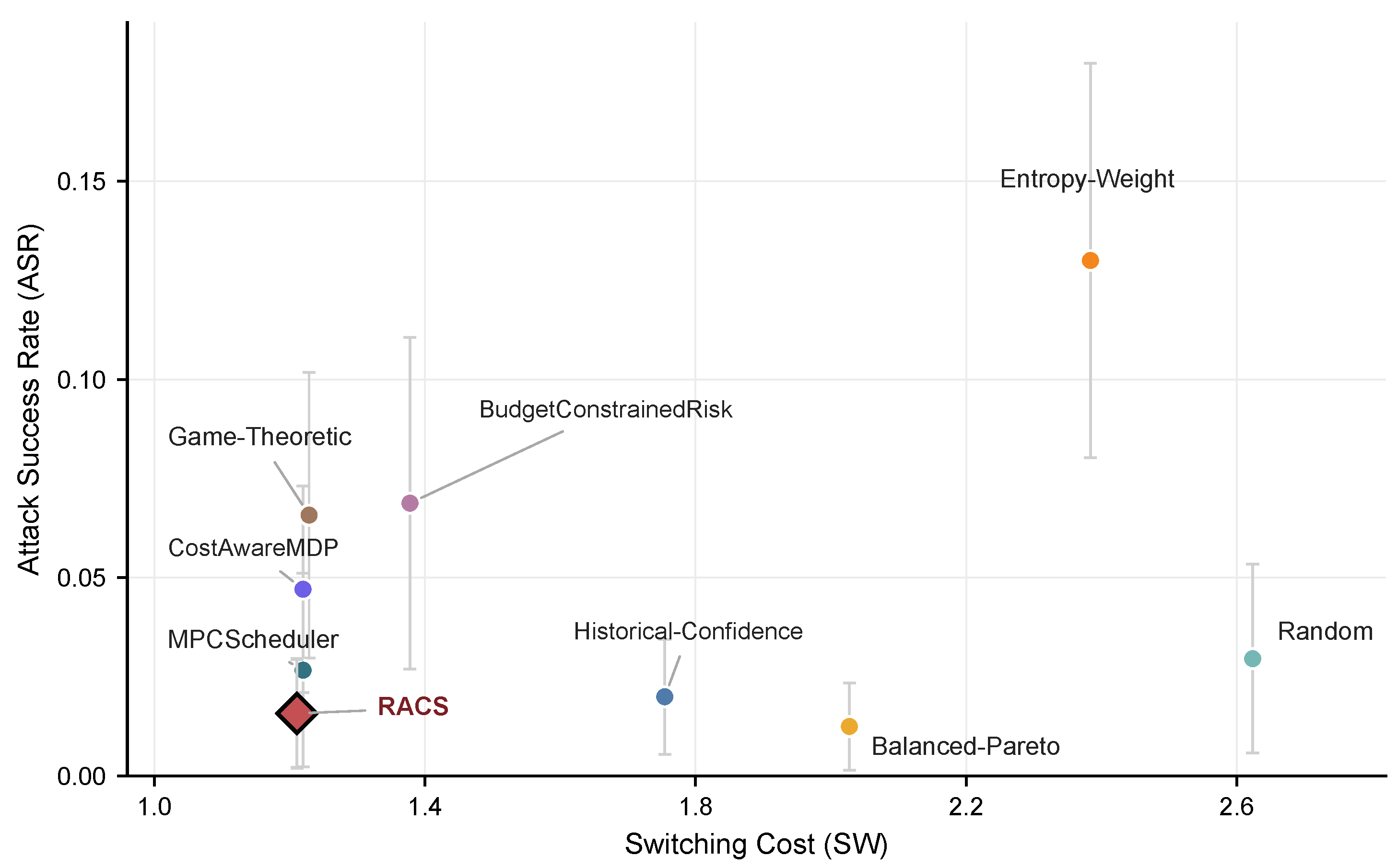
Figure 2 gives the risk–cost Pareto view under the burst-adaptive attacker. Points closer to the lower-left region correspond to lower attack success rate and lower switching cost. RACS is located in the low-ASR and low-SW region. Compared with CostAwareMDP, MPCScheduler, and Game-Theoretic scheduling, RACS achieves a lower ASR at a similar switching-cost level. Compared with Balanced-Pareto, RACS has a slightly higher ASR but a substantially lower switching cost. Therefore, Figure 2 visually illustrates the main role of RACS: it maintains a stable risk–cost trade-off under adaptive stress rather than minimizing only attack success or service-side cost.

The main comparison shows that RACS maintains consistent risk–cost behavior across the three attacker settings. Under the common-vulnerability setting, it suppresses common-vulnerability risk. Under the burst-adaptive setting, it avoids the joint triggering of high exposure and high common-vulnerability risk. Under the best-response adaptive setting, it maintains a balanced profile across ASR, SW, SLO, CV, and EXP. These results support the central claim of this paper: resource-constrained DHR executor-subset selection benefits from joint subset-level modeling of common-vulnerability risk, repeated exposure, and switching cost.

5.5. Parameter Sensitivity and Calibration Procedure

RACS involves two groups of parameters. The first group consists of the subset-scoring weights, including the heterogeneity weight ${\lambda }_h$, historical-confidence weight ${\lambda }_c$, cooldown-readiness weight ${\lambda }_r$, common-vulnerability-risk weight ${\lambda }_v$, exposure-penalty weight ${\lambda }_e$, and switching-cost weight ${\lambda }_s$. The second group consists of the exposure-memory update parameters, including the exposure decay factor $\rho$, the routine selection exposure gain $\alpha$, and the attack-related exposure gain $\beta$. These parameters jointly determine the scheduler’s preference among common-vulnerability risk, repeated visibility, and operational cost.

For a new deployment environment, RACS parameters can be selected using retained calibration traces or simulator-generated stress traces. Let

$$\theta =({\lambda }_h,{\lambda }_c,{\lambda }_r,{\lambda }_v,{\lambda }_e,{\lambda }_s,\rho ,\alpha ,\beta )$$

denote the complete RACS parameter vector, including both the subset-scoring weights and the exposure-memory update parameters. The operator first specifies system constraints, including an upper bound on switching cost $B_{\mathrm{sw}}$, an upper bound on SLO violation rate $B_{\mathrm{slo}}$, an upper bound on common-vulnerability risk $B_{\mathrm{cv}}$, and, when repeated visibility must be explicitly constrained, an upper bound on selected exposure $B_{\exp }$.

RACS is then evaluated over a finite candidate parameter set $\Theta$, and a fixed configuration is selected according to the risk–cost behavior observed on the calibration traces. A constrained calibration criterion can be written as

$${\theta }^{*}=arg\underset{\theta \in \Theta }{min}{\overline{\mathrm{ASR}}}_{\mathrm{cal}}\left(\theta \right),$$

(26)

subject to

$${\overline{\mathrm{SW}}}_{\mathrm{cal}}\left(\theta \right)\le B_{\mathrm{sw}},{\overline{\mathrm{SLO}}}_{\mathrm{cal}}\left(\theta \right)\le B_{\mathrm{slo}},{\overline{\mathrm{CV}}}_{\mathrm{cal}}\left(\theta \right)\le B_{\mathrm{cv}},{\overline{\mathrm{EXP}}}_{\mathrm{cal}}\left(\theta \right)\le B_{\exp }.$$

(27)

Here, ${\overline{\mathrm{ASR}}}_{\mathrm{cal}}$, ${\overline{\mathrm{SW}}}_{\mathrm{cal}}$, ${\overline{\mathrm{SLO}}}_{\mathrm{cal}}$, ${\overline{\mathrm{CV}}}_{\mathrm{cal}}$, and ${\overline{\mathrm{EXP}}}_{\mathrm{cal}}$ denote the mean attack success rate, switching cost, SLO violation rate, common-vulnerability risk, and selected exposure on the calibration traces, respectively. The exposure constraint is optional and is used when the deployment requires an explicit bound on repeated visibility. This procedure determines the operating parameters before deployment, and the selected configuration is kept fixed during test-time evaluation. The parameter sensitivity analysis characterizes the performance variation around the fixed configuration.

Table 5. One-factor parameter sensitivity summary under the burst-adaptive attacker. The complete sensitivity curves are reported in Appendix B.

Parameter	Swept Range	Default	Main Observation
${\lambda }_v$	0.50–2.50	1.50	CV decreases from 0.0148 to 0.0008, and ASR decreases from 0.0329 to about 0.0154–0.0175.
${\lambda }_e$	0.40–2.00	1.00	EXP decreases from 0.6646 to 0.5505, while SW and SLO increase.
${\lambda }_s$	0.05–0.75	0.45	At ${\lambda }_s=0.05$, SW reaches 2.0839; at ${\lambda }_s=0.75$, ASR increases to 0.0467.
$\rho$	0.80–0.97	0.92	EXP increases from 0.3047 to 1.2268; at $\rho =0.97$, ASR increases to 0.0333.
$\alpha$	0.06–0.24	0.12	EXP increases from 0.2775 to 1.1910, and ASR increases from 0.0179 to 0.0342.
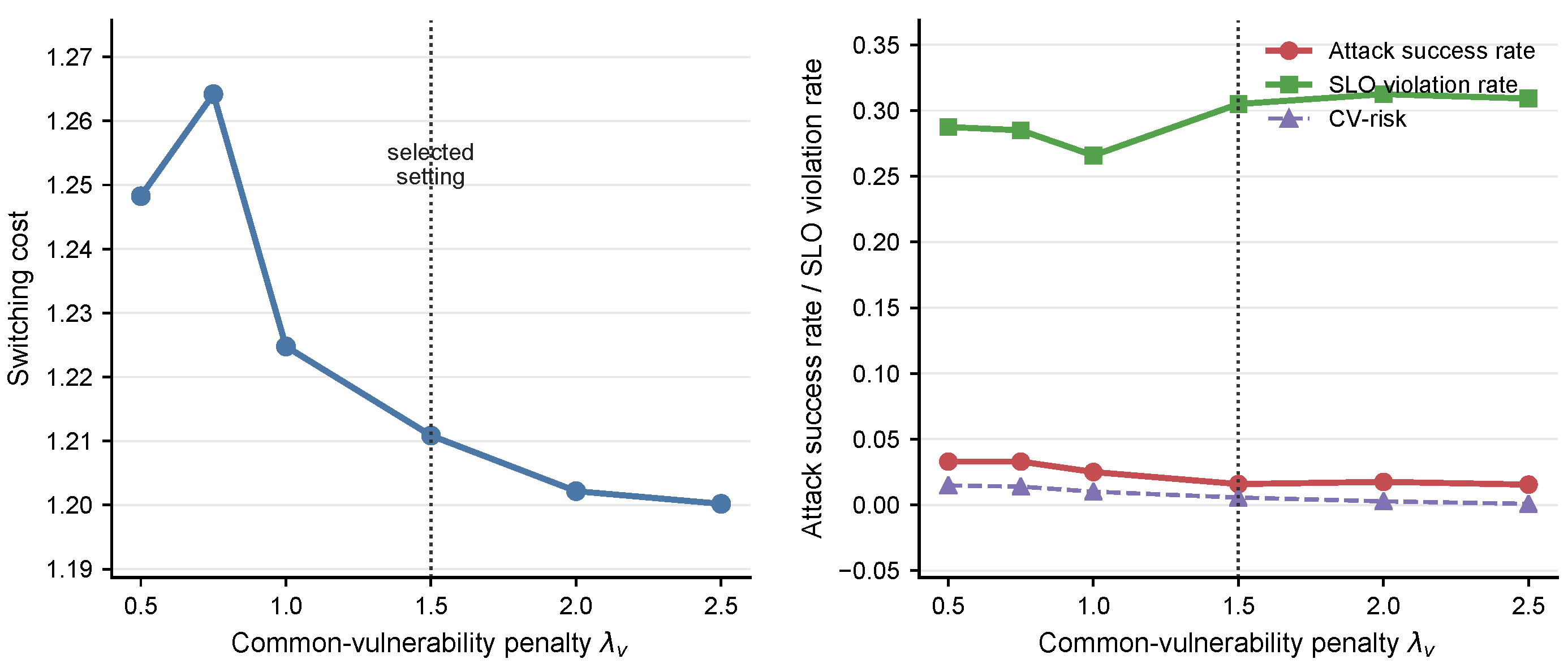
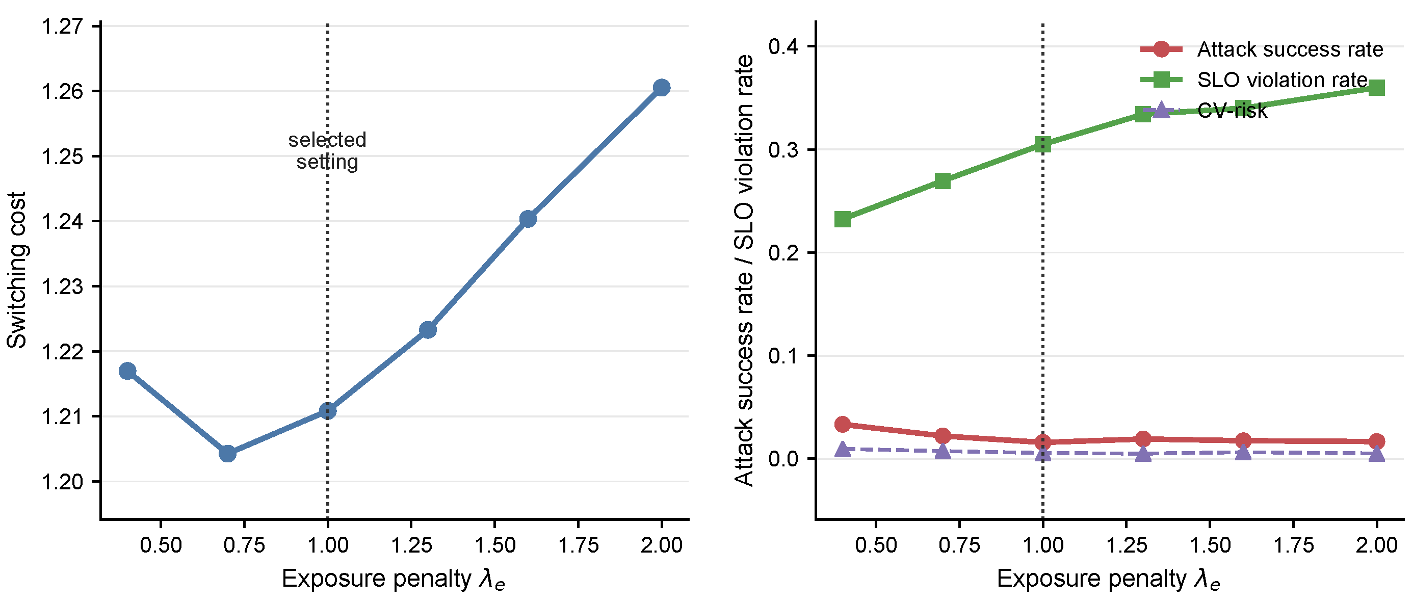
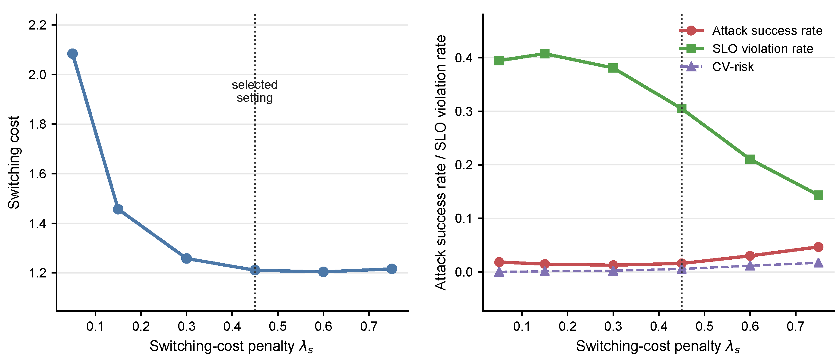
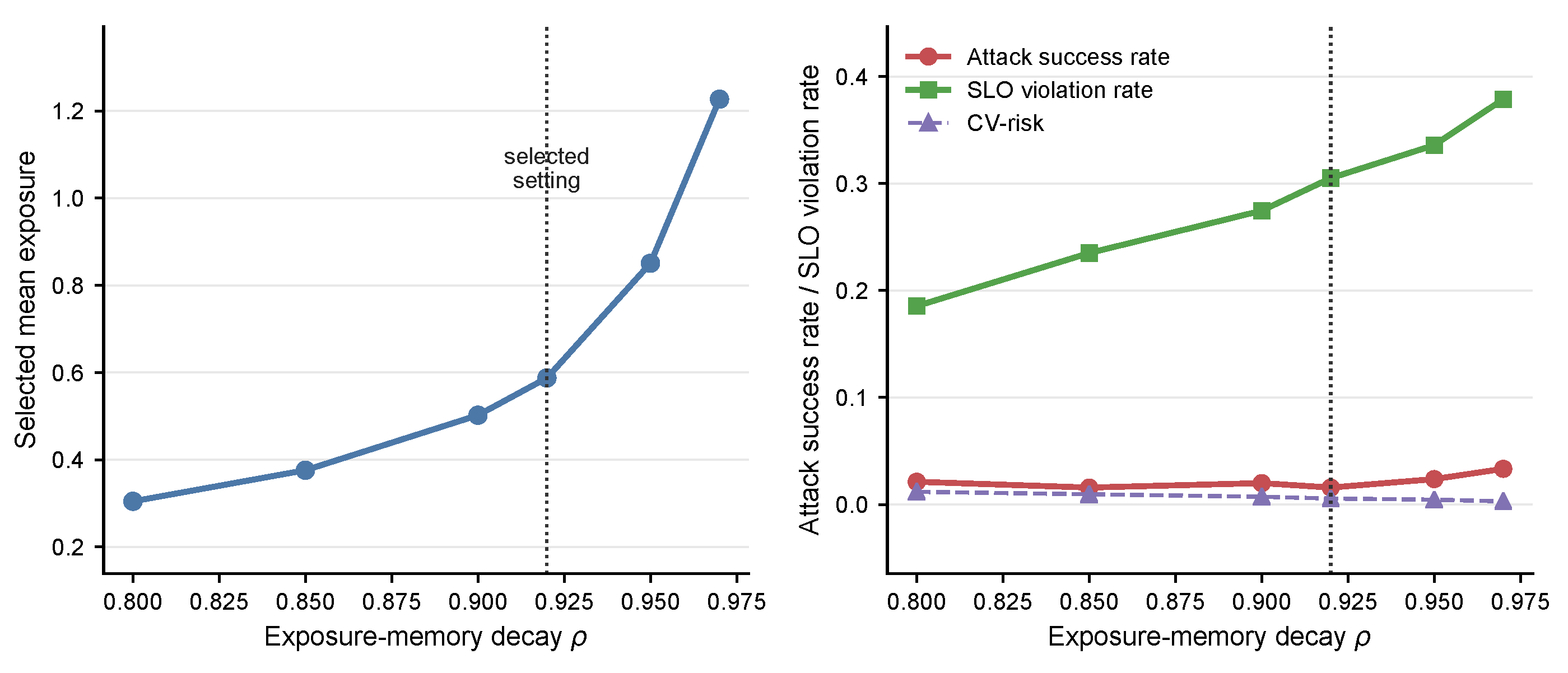
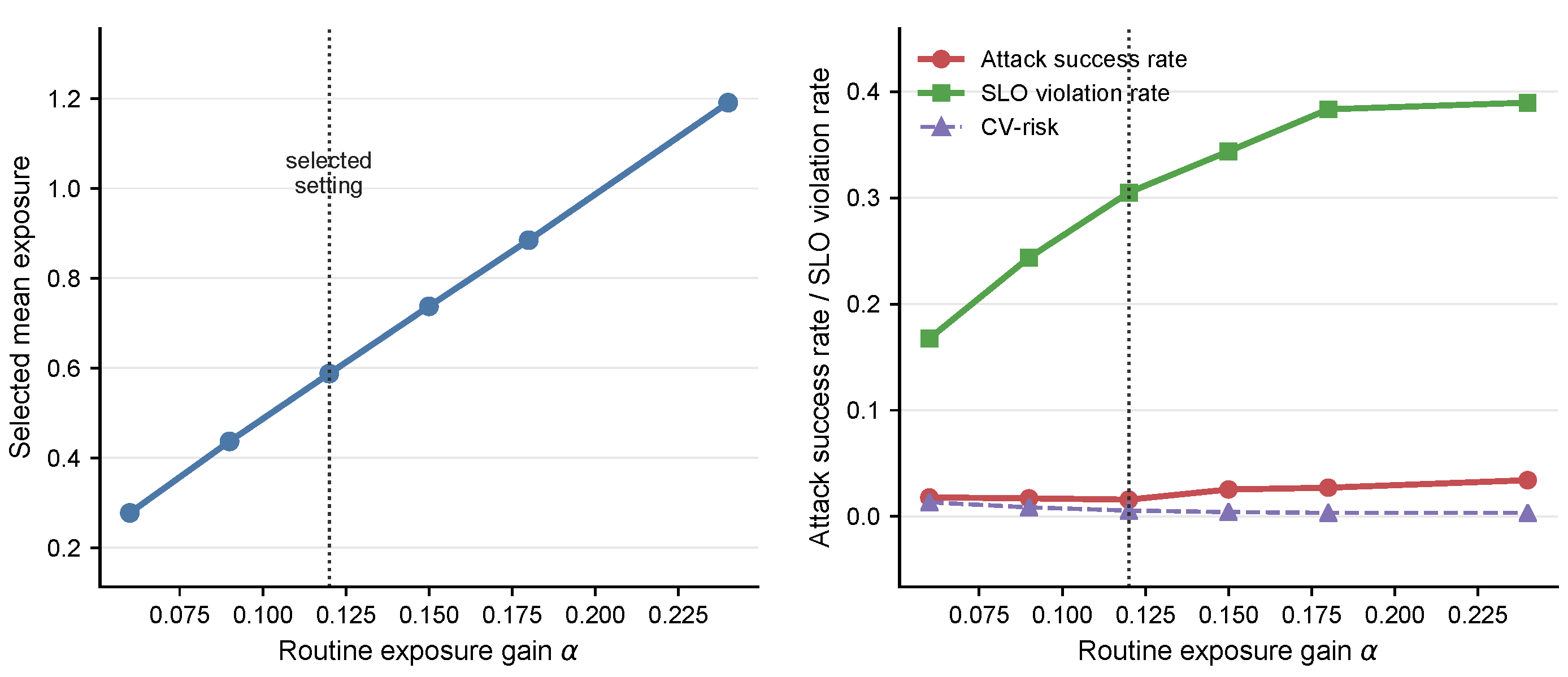
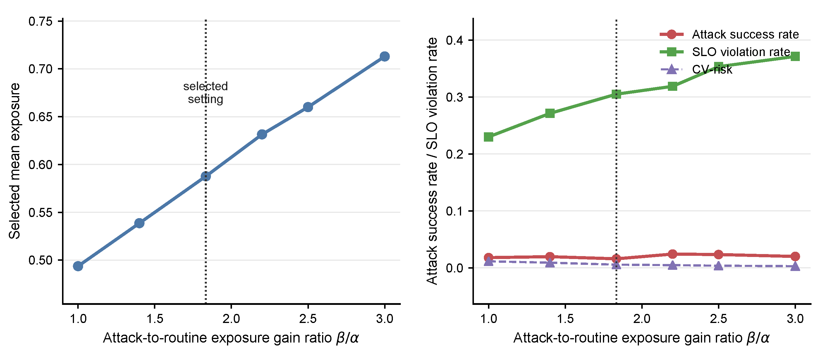
$\beta /\alpha$	1.00–3.00	1.83	CV decreases from 0.0114 to 0.0029, EXP increases from 0.4937 to 0.7130, and ASR remains lower near the default setting.

summarizes the six-point one-factor sensitivity results under the burst-adaptive attacker. In each experiment, only one parameter is varied, while the remaining parameters are kept at their default values. The results show that different parameters affect different aspects of the risk–cost trade-off. As ${\lambda }_v$ increases, CV decreases from 0.0148 to 0.0008, while ASR decreases from 0.0329 to approximately 0.0154–0.0175. The decrease in CV indicates that ${\lambda }_v$ primarily affects vulnerability-family overlap control. As ${\lambda }_e$ increases, EXP decreases from 0.6646 to 0.5505, while SW and SLO increase. The decrease in EXP indicates that ${\lambda }_e$ reduces repeated visibility, while the increases in SW and SLO show the accompanying switching and service disturbance. The parameter ${\lambda }_s$ has the most direct effect on the security–cost trade-off. When ${\lambda }_s=0.05$, SW reaches 2.0839; when ${\lambda }_s=0.75$, ASR increases to 0.0467. This result shows that a weaker switching penalty corresponds to higher switching cost, whereas a stronger switching penalty corresponds to higher attack success.

The results for the exposure-memory parameters $\rho$, $\alpha$, and $\beta$ should be interpreted together with the definition of EXP. EXP is a state variable generated by the exposure-memory recurrence, and its numerical scale is jointly determined by $\rho$, $\alpha$, and $\beta$. Under the same exposure-memory configuration, EXP can be used to compare the relative exposure levels produced by different schedulers. Across different exposure-memory parameter settings, EXP reflects changes in the scale and persistence of the defender-side repeated-visibility proxy. A larger $\rho$ extends the influence of historical exposure, a larger $\alpha$ amplifies visibility accumulation caused by routine selection, and a larger $\beta /\alpha$ increases the relative contribution of attack-related exposure in the state update.

Overall, the parameter sensitivity results characterize the risk–cost variation around the default configuration. The parameter ${\lambda }_v$ mainly affects common-vulnerability risk, ${\lambda }_e$ mainly affects repeated visibility and the resulting scheduling changes, and ${\lambda }_s$ mainly controls the trade-off between switching cost and risk avoidance. The parameters $\rho$, $\alpha$, and $\beta$ determine the persistence and gain scale of the exposure proxy state. The main experiments in this paper use a fixed default configuration. The complete one-factor sensitivity curves are reported in Appendix B.

5.6. Ablation Study

Table 6. The 20-seed stress ablation of the main RACS scoring terms under the burst-adaptive attacker. ASR, SW, and SLO are reported as mean ± standard deviation; CV and EXP are means.

Variant	ASR	SW	SLO	CV	EXP
RACS full	$0.0158\pm 0.0137$	$1.2109\pm 0.0519$	$0.3050\pm 0.0321$	0.0056	0.5877
Without common-vulnerability risk	$0.0496\pm 0.0227$	$1.2841\pm 0.0646$	$0.2817\pm 0.0336$	0.0217	0.6021
Without exposure	$0.0483\pm 0.0229$	$1.2069\pm 0.0602$	$0.1029\pm 0.0613$	0.0137	0.7792
Without switching cost	$0.0221\pm 0.0124$	$3.1936\pm 0.0463$	$0.4146\pm 0.0330$	0.0000	0.5289
Without confidence	$0.0221\pm 0.0157$	$1.2039\pm 0.0481$	$0.2704\pm 0.0406$	0.0060	0.5973

reports the ablation results under the burst-adaptive attacker. The full RACS obtains an ASR of $0.0158\pm 0.0137$, an SW of $1.2109\pm 0.0519$, an SLO violation rate of $0.3050\pm 0.0321$, a CV of 0.0056, and an EXP of 0.5877. Removing different scoring terms leads to different changes in security, cost, and mechanism metrics. The direction of these changes separates the effects of the common-vulnerability, exposure, switching-cost, and confidence terms.

After removing the common-vulnerability risk term, ASR increases from 0.0158 to 0.0496 and CV increases from 0.0056 to 0.0217. The paired seed-level interval supports a stable increase in ASR, with an ablation-minus-full difference of 0.0338 and a 95% interval of [0.0250, 0.0433]. It also supports a stable increase in CV, with a difference of 0.0161 and a 95% interval of [0.0144, 0.0178]. This result indicates that the common-vulnerability risk term directly contributes to avoiding shared vulnerability-family overlap. Without this term, vulnerability-family overlap within candidate subsets is no longer directly penalized. Selected subsets are then more likely to contain common-vulnerability overlap that can lead to correlated compromise.

After removing the exposure term, ASR increases from 0.0158 to 0.0483 and EXP increases from 0.5877 to 0.7792. The paired seed-level interval supports a stable increase in ASR, with a difference of 0.0325 and a 95% interval of [0.0242, 0.0417], and also supports a stable increase in EXP, with a difference of 0.1915 and a 95% interval of [0.1774, 0.2060]. At the same time, SLO decreases from 0.3050 to 0.1029, with a paired interval of [−0.2350, −0.1683]. This result reflects a trade-off between exposure control and service-side cost. Without the exposure penalty, the scheduler is more likely to repeatedly select low-latency and high-confidence executors, improving service-side indicators while increasing repeated visibility and attack success under burst-adaptive pressure.

After removing the switching-cost term, SW increases from 1.2109 to 3.1936 and the SLO violation rate increases from 0.3050 to 0.4146. The paired seed-level interval supports a stable increase in SW, with a difference of 1.9828 and a 95% interval of [1.9531, 2.0141], and also supports a stable increase in SLO, with a difference of 0.1096 and a 95% interval of [0.0892, 0.1275]. ASR also increases from 0.0158 to 0.0221, with a paired interval of [0.0017, 0.0108]. This result shows that additional movement does not automatically lead to better security outcomes. Without the switching-cost constraint, the scheduler changes executor subsets more frequently, substantially increasing operational disturbance while not improving attack success in this setting.

After removing the confidence term, ASR increases from 0.0158 to 0.0221. The paired seed-level interval supports a stable but smaller increase in ASR, with a difference of 0.0063 and a 95% interval of [0.0008, 0.0117]. SW, CV, and EXP change only moderately. This result suggests that historical confidence remains a useful complementary scheduling signal, but its marginal effect is smaller than those of the common-vulnerability risk and exposure terms in the current burst-adaptive stress setting.

The ablation study shows that the main RACS scoring terms act on different failure paths. The common-vulnerability risk term reduces majority compromise risk associated with shared vulnerability-family overlap; the exposure term controls the risk caused by repeated selection and repeated visibility; the switching-cost term constrains operational disturbance caused by scheduling movement; and the confidence term provides complementary historical reliability information. The advantage of the full RACS comes from the joint use of these signals rather than from any single metric alone.

5.7. Scalability and Resource-Budget Analysis

This section analyzes the cost behavior of RACS from two complementary perspectives. The first perspective is the scheduling overhead of the exact-enumeration implementation, namely the decision-time cost of evaluating candidate executor subsets at each round. The second perspective is switching-budget feasibility, namely whether a scheduler can maintain low attack success under explicit switching-cost constraints. The former characterizes the computational boundary of exact subset enumeration, while the latter characterizes the operational risk–cost behavior of RACS under resource budgets.

For an executor pool of size n and an active subset size k, the exact RACS implementation explicitly evaluates feasible candidate subsets. In the worst case, the number of candidates is $\left({\displaystyle \genfrac{}{}{0pt}{}{n}{k}}\right)$. Because heterogeneity and common-vulnerability overlap involve pairwise terms within each selected subset, the dominant scoring cost is approximately $O\left(\left({\displaystyle \genfrac{}{}{0pt}{}{n}{k}}\right)k^2\right)$ per scheduling round. This is the theoretical upper bound of the exact-enumeration implementation. In the simulator, cooldown and readiness constraints may reduce the number of available executors and therefore reduce the realized number of scored candidates.

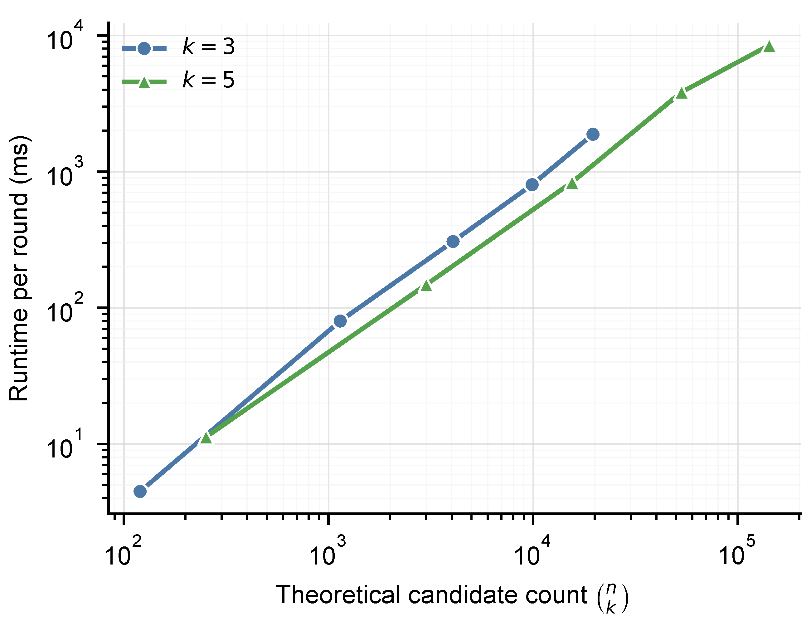
To characterize this computational boundary, we evaluate two subset-size settings. For $k=3$, the executor-pool size is set to $n=10,20,30,40,50$, with 20 seeds for each setting. For $k=5$, the executor-pool size is set to $n=10,15,20,25,30$, with 5 seeds for each setting. Each run contains 120 scheduling rounds. Figure 3 reports the representative per-round runtime from the same simulator implementation as a function of the theoretical number of candidate subsets.

Figure 3 shows that the runtime of exact RACS increases with the theoretical candidate count $\left({\displaystyle \genfrac{}{}{0pt}{}{n}{k}}\right)$. For $k=3$, the candidate count increases from $\left({\displaystyle \genfrac{}{}{0pt}{}{10}{3}}\right)=120$ to $\left({\displaystyle \genfrac{}{}{0pt}{}{50}{3}}\right)=19,600$, and the runtime increases from 4.4819 ms to 1882.3251 ms per round. For $k=5$, the candidate count increases from $\left({\displaystyle \genfrac{}{}{0pt}{}{10}{5}}\right)=252$ to $\left({\displaystyle \genfrac{}{}{0pt}{}{30}{5}}\right)=142,506$, and the runtime increases from 11.2673 ms to 8474.2124 ms per round. These results indicate that exact enumeration provides a transparent and executable implementation for small-to-medium DHR settings under the tested scheduling configuration. As the executor pool or active subset size further increases, scalable candidate-search mechanisms such as candidate pruning, cached pairwise feature matrices, greedy construction, beam search, stochastic candidate sampling, or parallel candidate scoring can be introduced.

In addition to scheduling overhead, resource constraints also appear through switching-cost budgets.

Table 7. Switching-cost budget feasibility under the burst-adaptive attacker. Feasibility is computed per seed according to whether the run-level mean switching cost is within the budget. Each cell reports feasible seeds out of 20, with the ASR averaged over feasible seeds in parentheses. CAMDP denotes CostAwareMDP, MPC denotes MPCScheduler, B-Pareto denotes Balanced-Pareto, and HistConf denotes Historical-Confidence.

Budget	RACS	CAMDP	MPC	B-Pareto	HistConf	Random
$B_{\mathrm{sw}}=1.25$	15/20 (0.0133)	15/20 (0.0400)	15/20 (0.0189)	0/20 (–)	0/20 (–)	0/20 (–)
$B_{\mathrm{sw}}=1.50$	20/20 (0.0158)	20/20 (0.0471)	20/20 (0.0267)	0/20 (–)	0/20 (–)	0/20 (–)
$B_{\mathrm{sw}}=2.00$	20/20 (0.0158)	20/20 (0.0471)	20/20 (0.0267)	3/20 (0.0139)	20/20 (0.0200)	0/20 (–)
$B_{\mathrm{sw}}=2.50$	20/20 (0.0158)	20/20 (0.0471)	20/20 (0.0267)	20/20 (0.0125)	20/20 (0.0200)	1/20 (0.0417)

reports a seed-level budget-feasibility check under the burst-adaptive attacker. A run is considered feasible when its run-level mean switching cost is no larger than the specified budget. At the strict budget $B_{\mathrm{sw}}=1.25$, RACS, CostAwareMDP, and MPCScheduler are feasible in 15 out of 20 seeds, while RACS has the lowest ASR among the feasible runs. When the budget is relaxed to $B_{\mathrm{sw}}=1.50$, all three methods are feasible in 20 out of 20 seeds, and RACS still achieves a lower ASR than CostAwareMDP and MPCScheduler. Balanced-Pareto becomes feasible in all seeds only when the budget is relaxed to $B_{\mathrm{sw}}=2.50$, where it obtains a lower ASR but requires a larger switching-cost budget. Historical-Confidence becomes feasible at $B_{\mathrm{sw}}=2.00$, but its ASR remains higher than that of RACS.

Overall, the runtime experiment characterizes the computational boundary of exact RACS, and the budget-feasibility experiment characterizes its behavior under explicit switching-cost constraints. Exact enumeration provides a transparent reference implementation for controlled evaluation and is executable for the tested small-to-medium settings. For larger deployments, the same RACS scoring rule can be paired with more scalable candidate-search procedures. The switching-budget results further show that RACS maintains low ASR under strict and moderate switching budgets, whereas several baselines either require relaxed budgets to become feasible or incur higher ASR at comparable budgets. These results support the role of RACS as an interpretable risk–cost scoring framework whose search component can be adapted to deployment scale.

5.8. Robustness to Vulnerability-Family Estimation Errors

RACS uses vulnerability-family overlap to estimate common-vulnerability risk. In practical deployments, these family labels may be inferred from SBOM records, dependency analysis, configuration similarity, or historical vulnerability reports, and such estimates can contain missing links or spurious links. To examine this source of uncertainty, we evaluate RACS under controlled vulnerability-family estimation errors and focus on the burst-adaptive attacker. Errors are injected only into the scheduler-side estimated pairwise vulnerability-family overlap relation used for computing the RACS common-vulnerability penalty. A noise rate q means that a fraction q of eligible pairwise relation entries is perturbed according to the corresponding error model: false-negative errors set sampled truly overlapping pairs to zero, while false-positive errors set sampled non-overlapping pairs to one. The attacker pressure, compromise simulation, and reported CV metric continue to use the ground-truth vulnerability-family structure, so the experiment isolates imperfect defender-side risk estimation from changes in the underlying attack model.

Table 8. Robustness of RACS to vulnerability-family estimation errors under the burst-adaptive attacker. Errors are injected into the scheduler-side estimated pairwise vulnerability-family overlap relation used by RACS; attacker pressure and the reported CV metric use the true vulnerability-family structure.

Error Model	Error Rate	ASR	SW	SLO	${\mathbf{CV}}_{\mathbf{true}}$	EXP	BA
clean	0.0	0.0158 ± 0.0137	1.2109 ± 0.0519	0.3050 ± 0.0321	0.0056	0.5877	0.0000
false-negative	0.1	0.0262 ± 0.0236	1.2309 ± 0.0720	0.2929 ± 0.0428	0.0095	0.5890	0.0000
	0.2	0.0238 ± 0.0138	1.2242 ± 0.0560	0.2833 ± 0.0411	0.0100	0.5928	0.0000
	0.3	0.0304 ± 0.0181	1.2550 ± 0.0441	0.2771 ± 0.0317	0.0136	0.5937	0.0025
false-positive	0.1	0.0212 ± 0.0166	1.2741 ± 0.0560	0.3596 ± 0.0414	0.0088	0.5847	0.0013
	0.2	0.0242 ± 0.0206	1.3794 ± 0.0798	0.3987 ± 0.0649	0.0151	0.5904	0.0063
	0.3	0.0279 ± 0.0213	1.5297 ± 0.1018	0.4429 ± 0.0702	0.0201	0.5764	0.0150
mixed	0.1	0.0279 ± 0.0140	1.2951 ± 0.0709	0.3346 ± 0.0757	0.0120	0.5872	0.0013
	0.2	0.0325 ± 0.0269	1.4089 ± 0.0975	0.3775 ± 0.0694	0.0172	0.5850	0.0100
	0.3	0.0350 ± 0.0234	1.5689 ± 0.0967	0.4179 ± 0.0805	0.0265	0.5816	0.0275

reports the clean setting and three representative error models. The clean row matches the current main RACS burst-adaptive row. Under false-negative errors, some true family overlaps are missed by the scheduler; ASR increases from 0.0158 to 0.0304 and true CV increases from 0.0056 to 0.0136 at error rate 0.3, while SW remains close to the clean setting. Under false-positive errors, the scheduler avoids spurious estimated overlaps, which increases switching and service disturbance; SW rises from 1.2109 to 1.5297 and SLO rises from 0.3050 to 0.4429 at error rate 0.3. However, because the estimated overlap no longer aligns well with the true common-vulnerability structure, true CV can still increase, reaching 0.0201 at error rate 0.3. Mixed errors combine both effects and produce the largest joint degradation in this table, with ASR 0.0350, true CV 0.0265, and BA 0.0275 at error rate 0.3. These results indicate limited degradation under mild-to-moderate vulnerability-family estimation errors. When the estimated family signal remains sufficiently aligned with the true common-vulnerability structure, the scheduler can still use the common-vulnerability penalty to avoid high-risk executor subsets. As the estimation noise increases, the results gradually reflect the expected boundary of this signal-dependent mechanism: the scheduling behavior becomes more conservative or less precisely aligned with the true vulnerability structure. In some cases, ASR, CV, or service-side cost increases.

6. Discussion

The main experimental results show that resource-constrained DHR scheduling is better understood as a problem of aligning scheduling signals with attacker-exploitable failure paths, rather than as a problem of simply maximizing movement frequency or heterogeneity. Different attacker settings correspond to different scheduling-induced risks. The common-vulnerability attacker exploits shared vulnerability-family structures among executors. The burst-adaptive attacker exploits the co-occurrence of repeated exposure and common-vulnerability risk. The best-response adaptive attacker further exploits historical scheduling tendencies that have already been observed. Together, these three stress settings show that a single scheduling signal cannot stably cover different sources of risk. Historical confidence, feature heterogeneity, exposure memory, common-vulnerability risk, and switching cost describe different aspects of the scheduling state, and their usefulness depends on whether they are aligned with attacker-exploitable failure paths.

The comparison with optimization-oriented baselines further clarifies the role of RACS. CostAwareMDP, MPCScheduler, Balanced-Pareto, and Game-Theoretic scheduling each reflect a reasonable defense principle, emphasizing service-side cost, short-horizon prediction, multi-objective balancing, or adversarial strategy selection, respectively. These methods can perform well on certain local objectives, such as reducing SLO violations, reducing local expected loss, or achieving lower attack success under a more relaxed switching-cost budget. The goal of RACS is not to dominate all baselines on every individual metric. Instead, RACS incorporates common-vulnerability risk, repeated exposure, and switching cost into the same candidate-subset scoring rule. The main value of RACS is to provide a transparent subset-level joint scoring method that keeps scheduling behavior aligned with the modeled failure paths under different attacker pressures.

The parameter analysis shows that the weights of RACS should not be interpreted as universal constants, but as an operating point selected before deployment according to system-specific risk–cost constraints. The calibration procedure in Section 5.5 formalizes this idea: parameters can be selected on retained calibration traces or simulator-generated stress traces under constraints on switching cost, SLO violation rate, and common-vulnerability risk, and the selected configuration is then kept fixed during testing or deployment. The sensitivity results show that different parameters correspond to different control directions in the risk–cost trade-off: ${\lambda }_v$ mainly affects vulnerability-family overlap control, ${\lambda }_e$ mainly affects repeated visibility and the resulting scheduling changes, and ${\lambda }_s$ controls the balance between switching cost and risk avoidance. Meanwhile, $\rho$, $\alpha$, and $\beta$ determine the persistence and gain scale of the defender-side exposure proxy state. This interpretation makes RACS configurable.

The ablation study further explains why the joint scoring structure is necessary. Removing the common-vulnerability term increases vulnerability-family overlap and attack success. The concurrent increases in vulnerability-family overlap and ASR indicate that feature diversity alone is insufficient when executors share exploitable vulnerability sources. Removing the exposure term increases the exposure level of selected executors and the attack success rate. The concurrent increases in selected exposure and ASR indicate that repeated visibility needs to be modeled separately from historical confidence. Removing the switching-cost term substantially increases switching cost and service disturbance, but does not automatically improve security. The resulting cost increase without an automatic security gain separates unconstrained movement from effective defense. Therefore, common-vulnerability overlap, repeated exposure, and switching-cost-induced service disturbance are three different failure paths and cannot be substituted by a single scheduling signal. The role of RACS is to map these failure paths to different scoring terms and jointly constrain them at the candidate-subset level.

The scalability and switching-budget analyses further clarify the implementation path of RACS. Exact enumeration provides a transparent and reproducible reference implementation and allows direct inspection of the risk–cost score for each candidate subset. It is therefore useful for validating the scheduling behavior induced by the scoring rule itself. Under the small-to-medium executor pools studied in this paper, this implementation covers the complete candidate space and clearly shows how executor-pool size, active subset size, and scheduling overhead are related. Larger-scale deployment does not change the RACS scoring principle, but requires pairing the same score with more efficient candidate-search mechanisms, such as candidate pruning, cached pairwise feature matrices, greedy construction, beam search, stochastic candidate sampling, or parallel scoring. The switching-budget analysis further shows that RACS does not rely on unconstrained high-frequency movement to obtain security benefits. Instead, it can maintain a low attack success rate under strict and moderate switching budgets. Thus, the core value of RACS lies in its interpretable subset-level risk–cost scoring rule, while the search strategy can be replaced or extended according to deployment scale.

The vulnerability-family estimation-error experiment further provides a deployment-level applicability boundary. In real systems, vulnerability-family relations usually need to be estimated from software bills of materials, dependency analysis, configuration similarity, runtime environments, or historical vulnerability records, and they are difficult to make perfectly accurate. The results show that limited false-negative, false-positive, and mixed estimation errors do not immediately destroy the risk–cost behavior of RACS, but they change its operating point in interpretable ways. False-negative errors hide true shared vulnerability relations and thus leave residual common-vulnerability risk. False-positive errors make the scheduler avoid spurious estimated overlaps and increase switching and service disturbance. Mixed errors combine both effects and lead to more pronounced degradation. This indicates that RACS does not require perfectly accurate vulnerability-family labels, but its common-vulnerability component depends on the estimated relations retaining useful alignment with the true common-vulnerability structure.

The results support a more general view of DHR scheduling: defensive movement is useful only when it changes attacker-relevant risk states at an acceptable operational cost. Executor diversity, historical reliability, repeated visibility, common-vulnerability risk, and switching overhead should be modeled as interacting but non-substitutable scheduling signals. The current study provides controlled simulation evidence, mainly for isolating and validating these mechanism effects. Future work should validate RACS on prototype DHR testbeds, measure deployment-level service disturbance and reconfiguration costs, and extend the threat model to attack-chain behaviors such as partial compromise, stealthy persistence, delayed exploitation, lateral movement, and attacks against the adjudication mechanism. It should also replace manually configured vulnerability-family sets with dependency-, configuration-, vulnerability-record-, or SBOM-derived relations, and integrate scalable candidate-search mechanisms for larger executor pools.

7. Conclusions

This paper presented RACS, a risk-aware and cost-constrained heuristic scheduling method for resource-constrained DHR systems. RACS scores candidate executor subsets by jointly considering heterogeneity, historical confidence, common-vulnerability risk, exposure memory, and switching cost. Together, these terms model DHR scheduling as a subset-level security–cost decision problem. We constructed a reproducible controlled simulation protocol and evaluated RACS through baseline comparison, parameter-sensitivity and calibration analysis, ablation study, scalability and switching-budget analysis, and vulnerability-family estimation-error robustness checks.

Across 20 random seeds, the results show that RACS provides consistent risk–cost behavior under common-vulnerability, burst-adaptive, and best-response adaptive stress settings. Under common-vulnerability pressure, RACS suppresses common-vulnerability risk while maintaining low switching cost. Under burst-adaptive pressure, it avoids the joint high-risk state formed by repeated exposure and common-vulnerability risk. Under best-response adaptive pressure, it remains competitive by jointly controlling attack success, common-vulnerability risk, repeated exposure, and switching cost. The ablation results further show that the common-vulnerability, exposure, and switching-cost terms constrain different failure paths, while the parameter and estimation-error analyses clarify the operating conditions and applicability boundary of the proposed scoring rule.

These findings support treating resource-constrained DHR scheduling as a joint decision problem over common-vulnerability risk, accumulated exposure, and operational cost, rather than relying only on heterogeneity maximization, historical confidence, periodic rotation, or movement-frequency control. Future work will validate the framework on prototype DHR testbeds, replace manually configured vulnerability-family sets with software-bill-of-materials, dependency, configuration-similarity, or vulnerability-record data, and develop scalable candidate-search strategies for larger executor pools.