Quantifying the Impact of Signal Simplification, Data Quantity, and Task Difficulty on Vision Transformer Performance for ECG Rhythm Classification

Abstract

Vision transformers (ViTs) have demonstrated considerable promise for classifying electrocardiogram (ECG) rhythms. However, much of the existing research is conducted in highly controlled, data-sterile settings that fail to reflect the substantial variability present in real-world ECG signals. This paper seeks to address this gap by examining how signal simplification, data quantity, and task difficulty influence the performance of the SwinV2 ViT model in ECG rhythm classification. Through systematic analysis, we highlight that classifying highly abstracted signals yields only a limited impact on model performance, with all models achieving over 95% accuracy, while the amount of training data plays a crucial role with an almost 15% accuracy difference between the models trained on the most data and the least data. Finally, our analysis shows the model’s ability to effectively adapt to an increased class count, which is essential due to the varying nature of ECG diagnosis. In summary, these results highlight the importance of carefully balancing data clarity, dataset size, and diagnostic variety when designing ECG classification systems. Achieving this balance is crucial for building reliable and scalable AI solutions for cardiac assessment.

1. Introduction

ECG signals present a unique challenge in both clinical and computational contexts due to their complexity and the wealth of information they contain. Although there have been extensive studies looking at the classification of ECG signals, these often lack data consistency and rarely reflect the unique challenges contained within this complex classification task. Although achieving high accuracy is crucial, it is equally important to recognize and account for the limitations inherent in real-world data. Understanding how these constraints affect model performance is essential for developing a robust and reliable diagnostic system.

1.1. Electrocardiograms

ECGs are graphical representations of the electrical activity of the heart and are essential tools in both clinical settings and medical research. However, the signals captured by ECG devices are complex and intricate, and therefore require considerable expertise to interpret accurately. For human readability, simplification techniques such as noise reduction and artifact removal are employed to enhance clarity [1].

The ECG recording process begins with the placement of electrodes on the skin at specific points on the chest and limbs to capture the heart’s electrical signals [2]. These electrodes detect the tiny electrical changes on the skin that arise from the heart during each heartbeat. The signals are then transmitted to an ECG machine, where they are amplified and filtered to remove any external electrical interference.

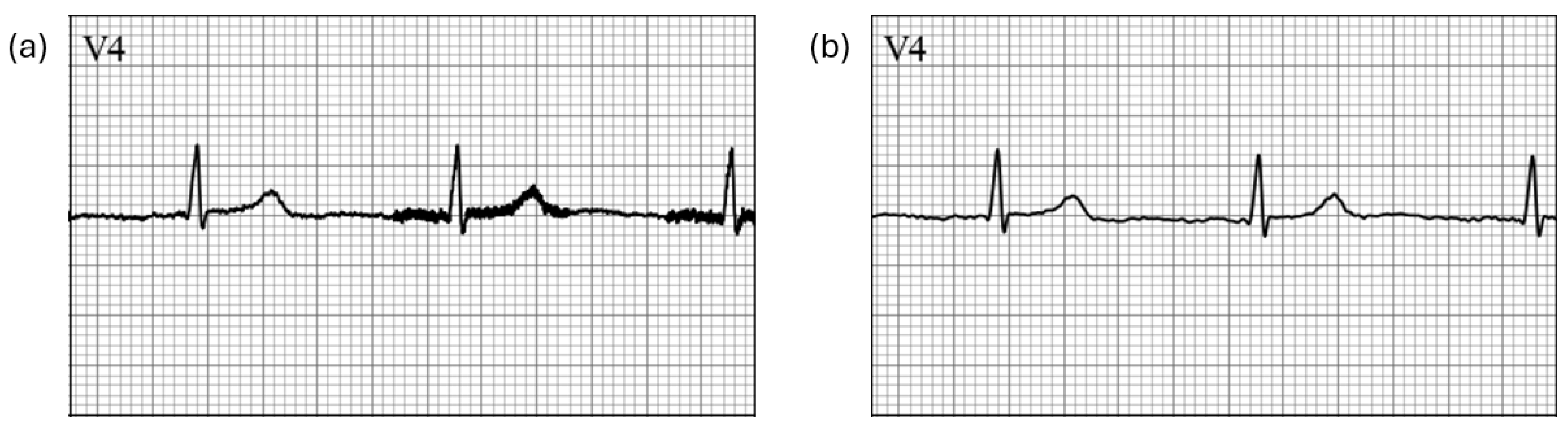
Once the raw signals are captured, they undergo digitization, converting the analogue signals into a digital format that can be processed by computers [3]. The digital signals are then subjected to further processing, such as baseline wander removal to correct any drift in the signal, and the elimination of power-line interference, see Figure 1. Advanced algorithms are used to enhance the signal quality and to extract meaningful features, such as the P wave, QRS complex and T wave, which are critical for diagnosing various cardiac conditions.

1.2. Proposal

In this paper we plan to explore the impact of data simplification for human readability on machine learning models. We intend to investigate how a simple signal enhancement technique, such as noise reduction, influences the accuracy and reliability of these models. By comparing models trained on raw versus increasingly simplified ECG signals, we aim to determine the extent to which simplification impacts the classification performance of the models. This section will also allow for the observation of how the model hands ‘broken’ or ‘incomplete’ data.

The amount of information extractable from an ECG is extensive; however, the broad range of diagnosable conditions and the various settings and in which an ECG can be recorded results in the classification task being extremely complex. Due to these challenges, acquiring large quantities of data is not always possible. Therefore, we will explore the importance of data quantity by using multiple models trained on progressively smaller datasets and review each model’s performance.

Most ECG classification models are trained to classify a small number of conditions [4,5,6]. While this helps to reduce variance by keeping the classification task simple, it is not reflective of reality as the variety of conditions diagnosable from an ECG is extensive. Therefore, to improve real-world fidelity we will utilize a 10-class dataset to train a model. While this is still far from being truly reflective, it will allow us an insight into how the model could handle a broader scope and an increased task difficulty.

2. Materials and Methods

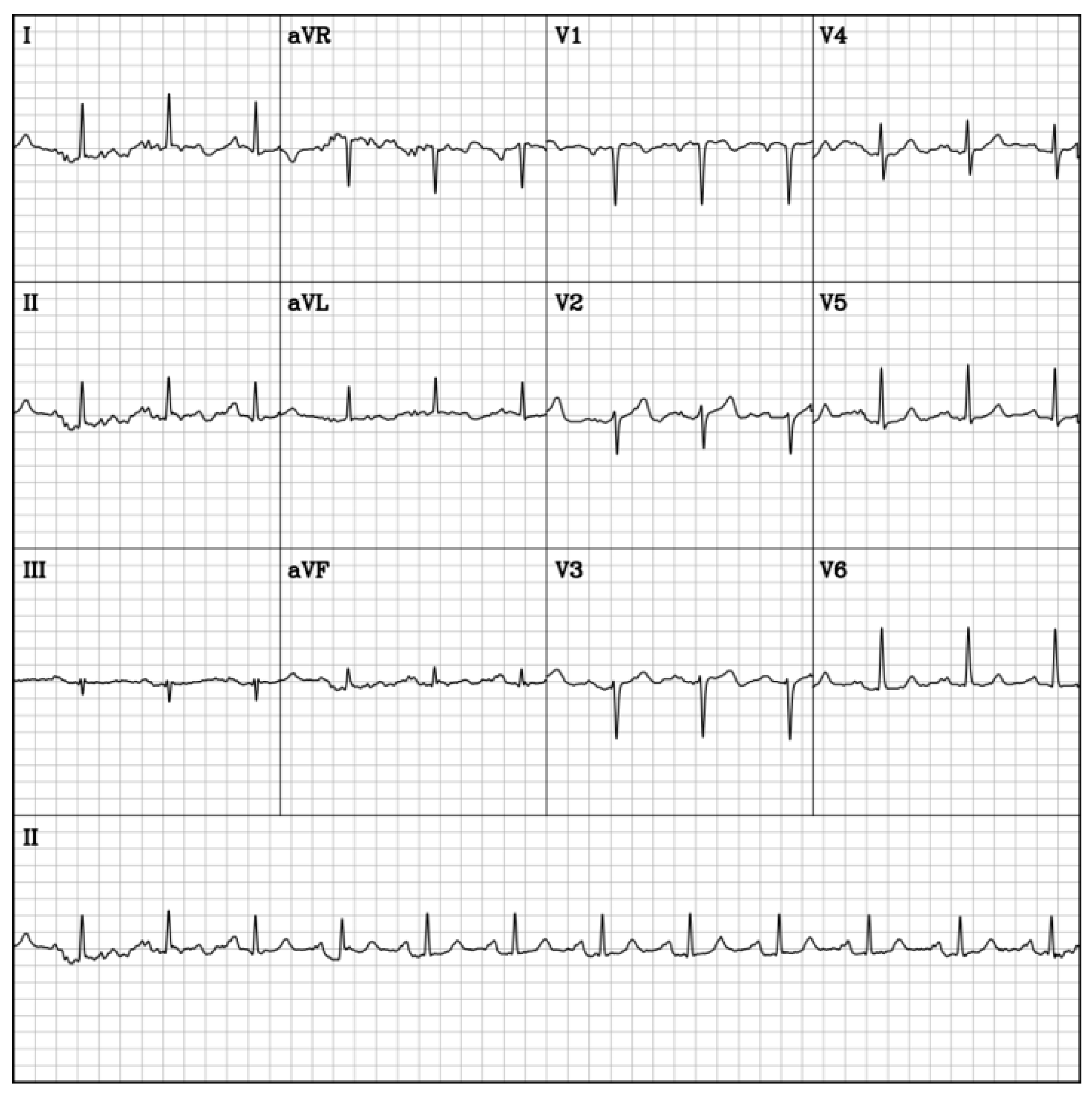
The SwinV2 vision transformer [7] was chosen due to its previous success classifying the MIMIC-IV-ECG dataset [8]. The model utilizes a shifted window approach to limit self-attention computation to non-overlapping local windows. This approach optimises efficiency and performance, especially when handling high resolution images. The model neatly divides the image into patches and windows. We chose to divide the images into 16 × 16 pixel patches and utilised a window size of 24 due to the divisions high overlap with the structure of a standard ECG, see Figure 2. With this configuration, each window corresponds to a single lead.

2.1. Dataset

The MIMIC-IV-ECG dataset is comprised of approximately 800,000 diagnostic ECGs that were collected from nearly 160,000 distinct patients [9,10]. Each ECG is recorded using 12 leads, spans 10 s, and is sampled at a frequency of 500 Hz. This extensive dataset encompasses all ECGs for patients present in the wider MIMIC-IV Clinical Database [10,11,12]. The dataset was chosen due to its extensive quantity of data that covers a substantial number of cardiac conditions and its high level of consistency.

2.2. Signal Simplification

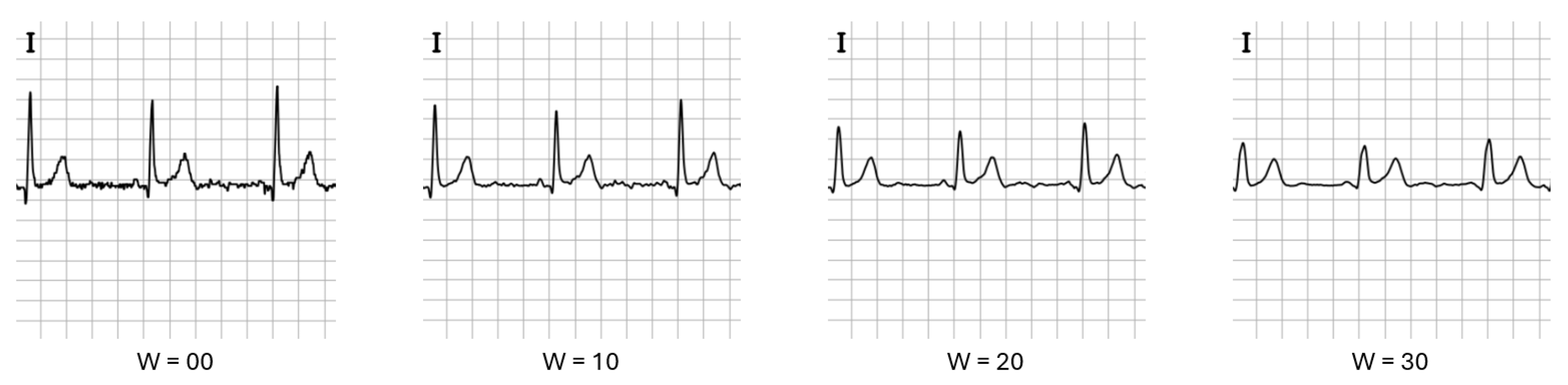
The Simple Moving Average (SMA) algorithm is a simple smoothing algorithm used to remove noise and minor artifacts from signals [13]. It is calculated by computing the unweighted average of the most recent observations within a specified window size. To simulate signal simplification, we used varying window sizes. As seen in Figure 3, the greater the window size (w), the simpler and more distorted the lead.

This method allowed us to incrementally mask features and, therefore, would allow us to observe model performance at observable thresholds. While the SMA algorithm is not used directly in normal ECG processing pipelines, it is a well established signal smoothing algorithm and acts as a computationally cheap and stable low pass filter that allows for direct, observable changes while still maintaining ECG morphology.

We selected the four most prominent diagnoses in the MIMIC-IV-ECG dataset—Sinus Rhythm, Sinus Bradycardia, Sinus Tachycardia, and Atrial Fibrillation—and extracted a total of 140,000 ECG recordings corresponding to these conditions. Each condition contributed 25,000 images to the training set, 5000 images to the validation set and a further 5000 images to the test set. These ECG recordings were then converted into image format for training on the SwinV2 vision transformer, as illustrated in Figure 2. This curated dataset was designated as c04-s140, indicating four conditions and a total of 140,000 samples.

We created four variations of the c04-s140 dataset, the variation w00 represented no signal simplification and the variations w10, w20 and w30 represented the number of neighboring nodes used to determine the average, see

Table 1. Table showing a breakdown of all the datasets used for training models.

Dataset	Window Size	No. of Classes	Training Data
c04-s140-w00	0	4	25,000
c04-s140-w10	10	4	25,000
c04-s140-w20	20	4	25,000
c04-s140-w30	30	4	25,000
c04-s70-w10	10	4	12,500
c04-s35-w10	10	4	6250
c04-s18-w10	10	4	3125
c10-s84-w10	10	10	6000
c04-s34-w10	10	4	6000

and Figure 3. We decided to limit the window size to 30 as extreme levels of masking of the P wave, QRS complex and T wave was present in w30.

Each of these models were trained for 100 epochs. Although training for more epochs might have yielded higher accuracies, computation time limited our ability to train further, and we believe 100 epochs produced sufficient data to establish trends. Furthermore, a ResNet-50 baseline was trained on the c04-s140-w10 dataset for a holistic analysis [14].

2.3. Data Count

To examine how data volume affects performance, three subsets were derived from the c04-s140-w10 dataset: c04-s70-w10, c04-s35-w10 and c04-s18-w10. The c04-s70-w10 subset contains exactly half the data count of c04-s140-w10, with the training, validation and test sets reduced to half their original size. Similarly, c04-s35-w10 and c04-s18-w10 contain a quarter and an eighth of the original data, with their training, validation and test sets reduced to a quarter and an eighth, respectively, of the initial count. For more details, see Table 1.

Unlike the c04-s140-w10 model, which was trained for 100 epochs, the c04-s70-w10, c04-s35-w10 and c04-s18-w10 subsets were trained for 150, 200 and 250 epochs respectively. This adjustment was made to observe whether increasing the number of training epochs could compensate for the reduction in available data. By extending the training duration, we aimed to assess if the models could achieve comparable performance despite having access to fewer samples, thereby providing insight into the interplay between data volume and training strategy.

The selected subset sizes were chosen to provide a clear, logical reduction in data volume, while also reflecting practical and achievable sample counts. To keep the dataset balanced, it is often necessary to make a substantial reduction in the amount of data per class. For example, when increasing the number of conditions from 4 to 10, the data per condition had to be reduced from 25,000 to 6000. This highlights the challenge inherent in ECG classification: while each condition holds equal significance, sufficient data for training models on every condition may not always be accessible.

2.4. Task Difficulty

To introduce a higher level of task complexity, the c10-s84-w10 dataset was created. Unlike the datasets described in the signal simplification and data count sections, which each featured 4 rhythm classes, c10-s84-w10 included 10 distinct rhythm classifications. However, as there is an inverse relationship between the number of rhythm types and the amount of data available for each, the training data per class was limited to 6000 samples, with an additional 1200 per class for validation and a further 1200 samples per class being allocated to the test set.

To directly observe how the step-up in difficulty impacted model performance, the c04-s34-w10 dataset was also created. It was designed to mirror the c10-s84-w10 dataset by containing the same number of samples per class, however instead of 10 classes, it only contains 4. Furthermore, a ResNet-50 baseline was trained on the c10-s84-w10 dataset to provide a more holistic analysis.

To remain in-line with the training regime applied to the other models, all models were trained for 100 epochs.

3. Results

3.1. Signal Simplification

ECG signals are highly susceptible to degradation and can be corrupted or distorted by various factors, including environmental noise, motion artifacts, and limitations inherent to the acquisition hardware. In this section, we investigate the impact of such signal distortions on model performance and evaluate the models’ robustness in scenarios where signal quality is not guaranteed. We will perform this analysis by examining four models that have been trained on signals exhibiting different levels of abstraction.

The top performing model, excluding the baseline, was c04-s140-w00 which achieved a top validation accuracy of 96.93%, see

Table 2. Table showing the validation accuracy, precision, recall and F1 score of the best performing epoch, based on validation accuracy and loss, for models c04-s140-w00, c04-s140-w10, c04-s140-w20, c04-s140-w30 and a ResNet-50 baseline trained on the c04-s140-w10 dataset.

Model	Epoch	Val Acc	Precision	Recall	F1
c04-s140-w00	99	96.93	0.972	0.972	0.972
c04-s140-w10	87	96.64	0.967	0.967	0.967
c04-s140-w20	97	96.31	0.964	0.964	0.964
c04-s140-w30	98	95.63	0.958	0.958	0.958
ResNet-50	18	97.10	0.971	0.971	0.9709

. This was closely matched by model c04-s140-w10 which recorded a validation accuracy of 96.64%. Model c04-s140-w20 was not far behind and achieved an accuracy of 96.31%. Finally, model c04-s140-w30, which had the highest level of signal simplification, performed significantly worse with a validation accuracy of 95.63%. While a trend indicating that higher levels of simplification leads to worse performance is visible, the impact appears to be nominal, with the difference between the best performing model, c04-s140-w00, and the worst performing model, c04-s140-w30, being only 1.30%. This indicates that for this set of rhythms, high levels of abstraction do not markedly affect the model’s ability to distinguish between diagnosis.

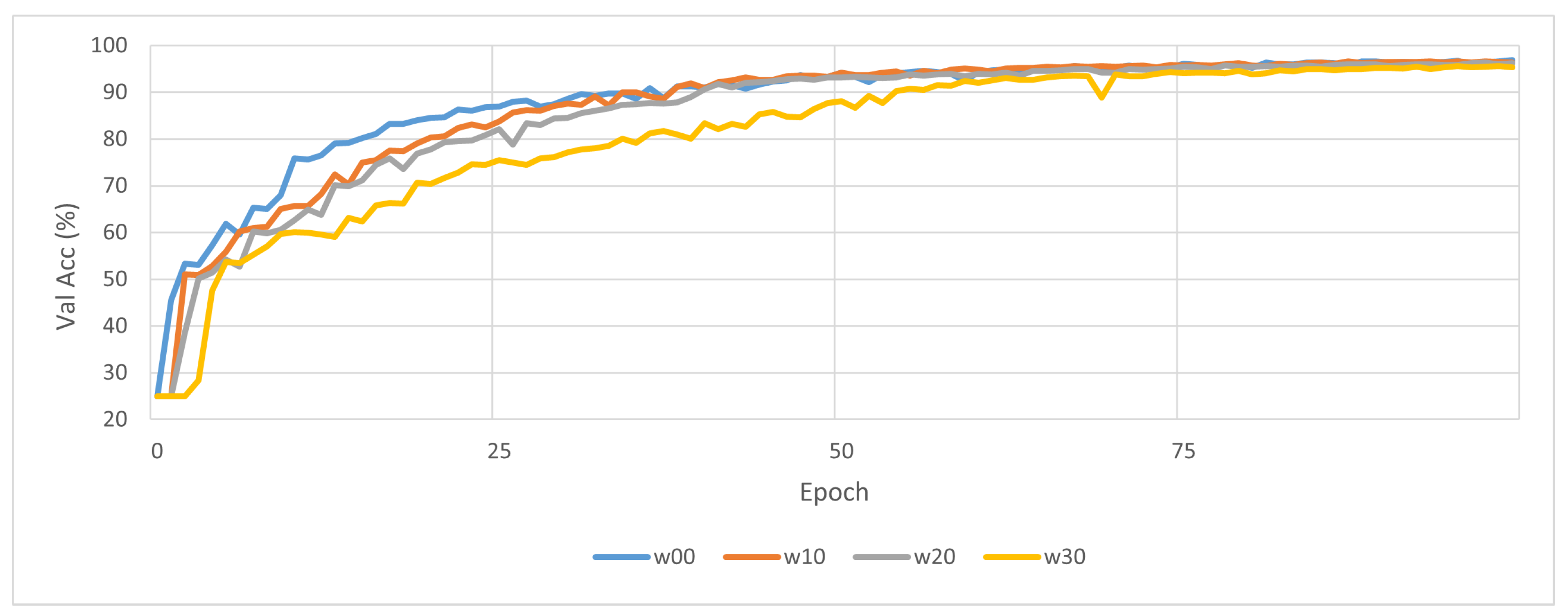
A more pronounced performance difference is illustrated in Figure 4, which presents the model’s validation accuracy as a function of training epochs. The graph highlights the substantial differences in performance among the models during the early training stages. Consistent with previous observations, configuration c04-s140-w00 achieves the highest accuracy, closely followed by c04-s140-w10 and c04-s140-w20, whereas c04-s140-w30 exhibits notably inferior performance. This disparity is particularly evident when looking at the convergence behavior. While models c04-s140-w00, c04-s140-w10, and c04-s140-w20 begin to converge around epoch 35, model c04-s140-w30 does not converge with the other models until approximately epoch 70.

While validation accuracy is an important baseline for observing and tracking training trends, its use in fine tuning model parameters can result in elevated performance metrics, therefore it is important to contextualize the validation accuracies using the test set, see

Table 3. Table showing the validation accuracy, validation loss, test accuracy and test loss of the best performing epoch, based on validation accuracy and loss, for models c04-s140-w00, c04-s140-w10, c04-s140-w20, c04-s140-w30 and a ResNet-50 baseline trained on the c04-s140-w10 dataset.

Model	Epoch	Val Acc	Val Loss	Test Acc	Test Loss
c04-s140-w00	99	96.93	0.2178	97.79	0.1947
c04-s140-w10	87	96.64	0.2241	97.5	0.1994
c04-s140-w20	97	96.31	0.237	97.26	0.2160
c04-s140-w30	98	95.63	0.2449	96.77	0.2173
ResNet-50	18	97.10	0.971	97.82	0.0750

.

Surprisingly, Table 3 shows the test set outperforming the validation set across all models. This may be due to a variety of reasons, however the most likely reason is that the test set contains a relatively easier set of diagnostic images, meaning less edge cases and more distinct samples. While it is possible that this may also be due to data-leakage, due to the use of sample-level data splitting, it is unlikely as the elevated performance would be present in both sets. Nevertheless, the high level of performance on the test set indicates that the model is generalizing well.

Overall, the disparity in performance, coupled with observations of the model’s final behavior, suggests that although the impact of simple simplification is minimal in later training stages, it can still influence the model’s capacity to establish well-defined decision boundaries for classification, potentially necessitating additional training to reliably identify discriminative features. It is important to emphasize that, although the selected rhythms are generally distinct, borderline cases are present and may adversely affect performance. Consequently, the measured accuracy, in the later stages, is more indicative of the model’s ability to differentiate between those subtle, closely related instances.

3.2. Data Count

Diagnosing an ECG is a complex task that relies on interpreting both local and global features. Clinicians must draw on substantial experience and remain adaptable as they assess and label an ECG. Given the wide range of possible diagnoses and the layered complexity of ECG reports, it is almost impossible to gather large quantities of data for every diagnosis. As a result, models trained for ECG classification are often limited to a smaller set of conditions or must utilize imbalanced datasets for training. This makes it crucial to understand the impact of data quantity on a model’s ability to accurately interpret and classify ECGs.

To fully understand the impact of data quantity, we took a relatively simple diagnostic problem that looked at the classification of four distinct rhythms—Sinus Rhythm, Sinus Bradycardia, Sinus Tachycardia, and Atrial Fibrillation—and trained four models with different data quantities, ranging from 25,000 units of training data per class to 3125 units of training data per class, see Table 1 and

Table 4. Table showing the accuracy, precision, recall and F1 score of the best performing epoch, based on accuracy, before or at epoch 100, for models c04-s140-w10, c04-s70-w10, c04-s35-w10 and c04-s18-w10.

Model	Epoch	Val Acc	Precision	Recall	F1
c04-s140-w10	87	96.64	0.967	0.967	0.967
c04-s70-w10	99	90.93	0.911	0.910	0.909
c04-s35-w10	98	76.72	0.766	0.768	0.759
c04-s18-w10	93	64.08	0.604	0.636	0.598

.

We initially trained all four models for a total of 100 epochs and saw an immediate trend, see Table 4. The model with the most training data per class, c04-s140-w10, significantly outperformed the other three models and obtained an accuracy of 96.64%. Model c04-s70-w10 followed with a notable accuracy of 90.93% and subsequently models c04-s35-w10 and c04-s18-w10 were the worst performing models with respective accuracies of 76.72% and 64.08%. This shows the direct impact of data quantity: the more data, the higher the accuracy.

Although a clear trend did present itself, we wanted to see if the loss in accuracy could be overcome by training the model for additional epochs. Therefore, we trained c04-s70-w10 for an additional 50 epochs, c04-s35-w10 for an additional 100 epochs and c04-s18-w10 for an additional 150 epochs, see

Table 5. Table showing the validation accuracy, precision, recall and F1 score of the best performing epoch, based on accuracy, for models c04-s140-w10, c04-s70-w10, c04-s35-w10 and c04-s18-w10.

Model	Epoch	Val Acc	Precision	Recall	F1
c04-s140-w10	87	96.64	0.967	0.967	0.967
c04-s70-w10	146	94.26	0.946	0.946	0.946
c04-s35-w10	195	88.42	0.887	0.887	0.887
c04-s18-w10	247	81.88	0.823	0.823	0.823

.

On initial observation of Table 5, it becomes apparent that the accuracy of each model improved significantly with the additional training time. While this improvement was not sufficient to allow for any of the models to catch up with c04-s140-w10, the performance disparity was greatly reduced. This is particularly notable with model c04-s70-w10 as the additional 50 epochs allowed for an improvement of $\tilde{4}\%$ to an overall accuracy of 94.26%. Models c04-s35-w10 and c04-s18-w10 follow this trend with a increase of $\widetilde{12}\%$ and $\widetilde{17}\%$ respectively. This is coupled with an increase in stability, indicated by the Precision, Recall and F1.

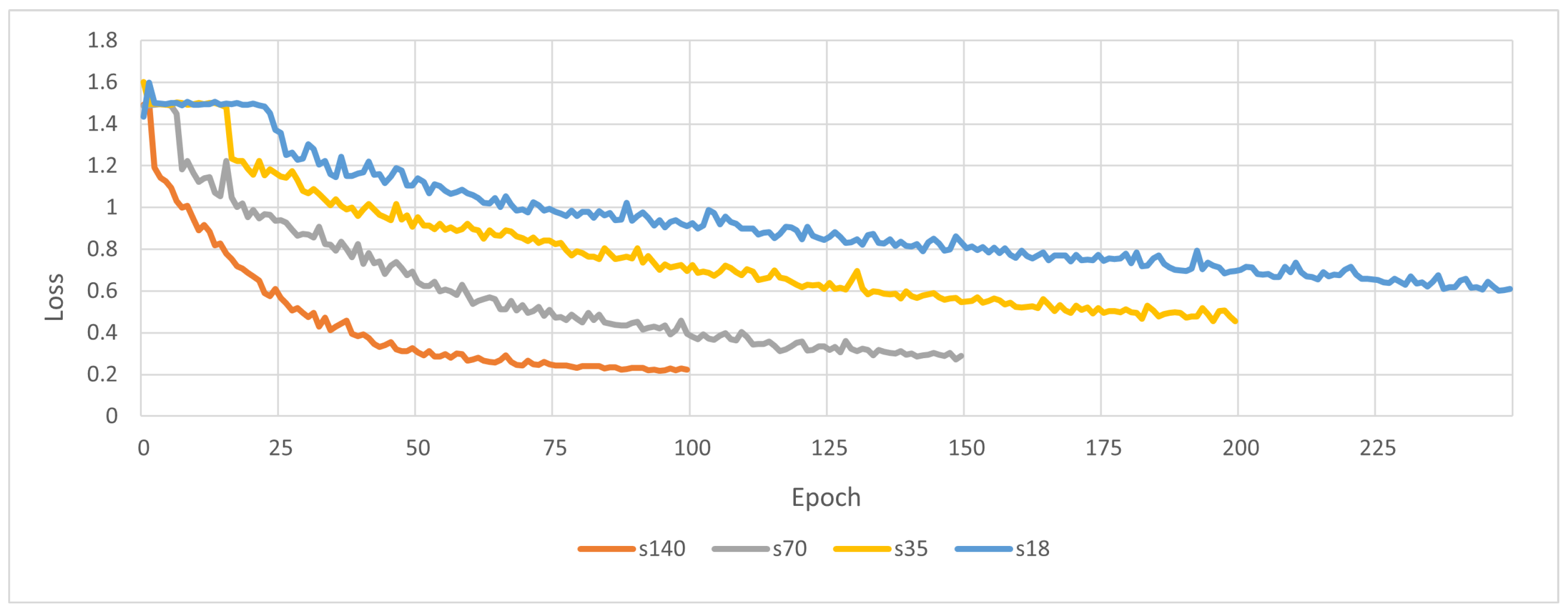
While additional training may be able to supplement data quantity, it can also lead to overfitting, therefore to provide a comprehensive evaluation of each model’s performance, we examined the training and validation loss of the best performing epoch for each model, see

Table 6. Table showing the loss difference at the best performing epoch, based on validation accuracy and loss, for models c04-s140-w10, c04-s70-w10, c04-s35-w10 and c04-s18-w10.

Dataset	Epoch	Val Loss	Train Loss	Difference
c04-s140-w10	87	0.2141	0.0483	0.1758
c04-s70-w10	146	0.2885	0.0517	0.2368
c04-s35-w10	195	0.4549	0.0582	0.3967
c04-s18-w10	247	0.6020	0.0606	0.5414

and Figure 5.

While there are no clear signs of underfitting or overfitting, Table 6 and Figure 5 show that the models are at very different stages of training. As observed in Figure 5, the loss curve of c04-s140-w10 has begun to plateau, indicating that further, substantial improvement is unlikely. However the loss curves for c04-s70-w10, c04-s35-w10 and c04-s18-w10 appear to still be trending downwards. This is supported by Table 6 which shows a substantially higher validation-train loss difference for models c04-s70-w10, c04-s35-w10 and c04-s18-w10 compared to c04-s140-w10’s difference of 0.1758. These observation suggests that the previously reported differences in accuracy may primarily reflect disparities in training-stage progression, and that a substantially greater number of epochs is required for models trained on smaller datasets to achieve competitive performance. However, given the gradient of models c04-s35-w10 and c04-s18-w10’s loss curves, it is unlikely they will fully catch up.

Finally, we compared each models performance on their respective validation and test sets to observe if the lower training data count affected the model’s ability to generalize to unseen data, see

Table 7. Table showing the validation accuracy, validation loss, test accuracy and test loss of the best performing epoch, based on validation accuracy and loss, for models c04-s140-w10, c04-s70-w10, c04-s35-w10 and c04-s18-w10.

Model	Epoch	Val Acc	Val Loss	Test Acc	Test Loss
c04-s140-w10	87	96.64	0.2241	97.50	0.1994
c04-s70-w10	146	94.26	0.2885	95.56	0.2603
c04-s35-w10	195	88.42	0.4549	89.26	0.4511
c04-s18-w10	247	81.88	0.6020	82.44	0.6046

. Upon examination, the models appear to have no issues with classifying the test sets, with all four models performing better on the test sets than than the validation sets. While model c04-s18-w10 did perform slightly better, with respect to loss, in the validation set, the difference was negligible and not a point of any major concern.

3.3. Task Difficulty

The classification of ECG rhythms is an inherently complex problem. This is primarily due to the large number of diagnostic categories and the subtle morphological and temporal features that distinguish them. Paradoxically, ECG classification models are often trained on a limited subset of conditions. This restricted label space fails to accurately reflect clinical reality where a broad spectrum of diagnostic labels and patterns can be encountered. In this section, we investigate how increasing task complexity, by expanding the number of conditions considered by the model from 4 to 10, impacts the models overall performance.

This escalation in task difficulty from a constrained, low-dimensional label space to a more comprehensive one is analogous to the progression experienced by medical students as they move from classroom-based learning to clinical practice. In contrast to the challenges often faced by trainees during this transition, the ViT demonstrates robust performance under the increased task complexity, achieving an accuracy of 83.98%. This result underscores the model’s adaptability and its capacity to scale to a larger and more heterogeneous set of diagnostic categories, see

Table 8. Table showing the accuracy, precision, recall and F1 score of the best performing epoch, based on validation accuracy, for models c04-s140-w10, c10-s84-w10, c04-s34-w10 and a ResNet-50 baseline trained on the c10-s84-w10 dataset.

Model	Epoch	Val Acc	Precision	Recall	F1
c04-s140-w10	87	96.64	0.967	0.967	0.967
c10-s84-w10	98	83.28	0.834	0.834	0.833
c04-s34-w10	99	80.98	0.809	0.807	0.800
ResNet-50	18	88.78	0.888	0.888	0.888

.

Although c10-s84-w10 fails to obtain the same level of accuracy as model c04-s140-w10, which obtained an accuracy of 96.64%, the accuracy relative to chance is still impressive. It is also important to remember that due to the increased condition count, a lower data per class had to be used for training. From the previous section we have already established that decreasing the training data quantity per class directly affects the model’s ability to learn. While this can be overcome by increasing the number of epochs the model is trained for, it does not fully compensate for the data loss, see Table 4 and Table 5.

To better isolate the difficulty step-up and remove the influence of the additional training samples per class, the c04-s34-w10 dataset was created to mirror the data conditions of c10-s84-w10. This means that c04-s34-w10 contained the same number of images per class for the training, validation and testing sets; however, instead of 10 rhythm classes, it contained only 4 rhythm classes, for more details see Table 1.

When comparing models c04-s34-w10 and c10-s84-w10, we see that despite the increase in rhythms types, c10-s84-w10 outperforms c04-s34-w10 with a validation accuracy of 83.28% compared to c04-s34-w10’s accuracy of 80.98%, see Table 8. This should be due to the fact that even though c10-s84-w10 had a lower class count compared to c04-s34-w10 and both shared the same quantity of samples per class in each split, the overall data count was higher due to the increased class count. This shows that while increasing the class count does affect the accuracy, it can also result in a slight uptick in performance due to the overall increase in data.

To verify if this trend extends to unseen data, we compared the validation accuracy and loss to the test accuracy and loss.

Table 9. Table showing the validation accuracy, validation loss, test accuracy and test loss of the best performing epoch, based on validation accuracy and loss, for models c04-s140-w10, c10-s84-w10, c04-s34-w10 and a ResNet-50 baseline trained on the c10-s84-w10 dataset.

Model	Epoch	Val Acc	Val Loss	Test Acc	Test Loss
c04-s140-w10	87	96.64	0.2241	97.50	0.1994
c10-s84-w10	98	83.28	0.6204	85.88	0.5312
c04-s34-w10	99	80.98	0.6337	79.96	0.6574
ResNet-50	18	88.78	0.3569	89.02	0.3767

not only shows that c10-s84-w10 outperforms c04-s34-w10 on unseen samples, but emphasizes that it outperforms it by a significant margin. This appears to indicate that in situations where low per class data is available, increasing the number of classes, and therefore the total sample count, could result in a better, more stable model.

Furthermore, despite model c10-s84-w10’s precision, recall, and F1 score being closely aligned, they diverge slightly from the overall accuracy, suggesting potential class-wise variability, see Table 8. This may just be statistical noise; however, further investigation into per-class performance is required, see

Table 10. Table showing the per class accuracy breakdown for the best performing epoch, based on validation accuracy and loss, of model c10-s84-w10.

Class	Rhythm	Accuracy
0	Atrial Fibrillation	85.5
1	Atrial Fibrillation with Rapid Ventricular Response	63.0
2	Sinus Arrhythmia	76.0
3	Sinus Bradycardia	96.5
4	Sinus Rhythm	68.5
5	Sinus Rhythm with 1st Degree A-V Block	82.7
6	Sinus Rhythm with borderline 1st Degree A-V Block	70.3
7	Sinus Rhythm with PAC(s)	80.3
8	Sinus Tachycardia	97.5
9	Ventricular Pacing	94.8

.

Table 10 clearly illustrates substantial variability in classification performance across the different classes. While several classes achieve relatively high accuracies exceeding 90%, the overall classification accuracy is markedly reduced by a small subset of poorly performing classes. The most prominent examples are classes 1, 2, 4 and 6, which attain accuracies of only 63%, 76%, 68.5% and 70.3%, respectively.

Although these values are considerably lower than the other rhythm classes, the poor performance is understandable when the class definitions are mapped to their corresponding cardiac rhythms. For example, class 6 corresponds to the arrhythmia “Sinus Rhythm with borderline 1st Degree A-V Block”, a rhythm which has high overlap with class 5, which corresponds to “Sinus Rhythm with 1st Degree A-V Block”. As these two rhythms are clinically very similar, with substantial overlap in their characteristics, an increased rate of misclassification between them is to be expected. It is also conceivable that, if the model were trained for a longer duration or with more stringent decision boundaries, it might develop a more discriminative internal representation, thereby improving the separability of these two closely related conditions and improving overall accuracy.

The other poorly performing classes 1, 2, and 4, correspond to “Atrial Fibrillation with Rapid Ventricular Response”, Sinus Arrhythmia, and Sinus Rhythm respectively. While the lower accuracy of class 2 can be explained by the subtle nature of Sinus Arrhythmia, it is surprising to see classes 0 and 4 under perform, given the transformer’s previous success in classifying both Atrial Fibrillation and Sinus Rhythm.

Several factors could contribute to this unexpected result, but the most plausible explanation is the presence of noise within the dataset and the limited training time. Furthermore, both classes have significant overlap with other conditions in the dataset, which can complicate classification. It is also important to recognize that the class labels were assigned using machine measurements, meaning the model’s accuracy is ultimately dependent on the machine’s ability to correctly categorize the ECGs. Consequently, any limitations or errors in the initial machine labeling will inevitably impact the overall performance of the classification model. Unfortunately, this is a well-documented issue within the field of medical imaging classification and while steps can be taken to limit data poisoning, it is near impossible to fully eliminate it.

4. Discussion

4.1. Signal Simplification

The training results for models c04-s140-w00, c04-s140-w10, c04-s140-w20, and c04-s140-w30, see Table 2 and Figure 4, reveal a clear trend: increasing the degree of simplification leads to a deterioration in performance. However, although this trend is evident, its overall impact on performance is minimal as all models achieve an accuracy of over 95%. While this may suggest that signal quality may have less effect on models compared to humans, it is important to contextualize that this training occurred in a controlled, sterile environment with a limited number of simple rhythms.

This is important to remember as the rhythms chosen for this experiment; Sinus Rhythm, Sinus Bradycardia, Sinus Tachycardia and Atrial Fibrillation, where chosen for their frequency, not complexity, and can be distinguished from one another without intricate analysis of the QRS complex. Therefore, while high levels of abstraction may have limited impact for this set of rhythms, it may not be the case for all sets of rhythms, meaning image and signal quality should still be maintained to a high degree.

It should also be noted that, for the selected set of rhythms, model performance is somewhat suboptimal. Although the rhythms are related, they constitute a group of distinct and relatively simple rhythms, that even less experienced clinicians would typically be able to differentiate with ease. While this might suggest that ViTs are not well suited to ECG analysis, it is more plausible that the models are struggling with borderline cases.

For example, Sinus Bradycardia is conventionally defined as a resting heart rate of fewer than 60 beats per minute, whereas Sinus Rhythm is defined as a resting heart rate between 60 and 100 beats per minute. Consequently, a resting heart rate of 59 beats per minute would be classified as Sinus Bradycardia, despite being morphologically and functionally very similar to Sinus Rhythm. These borderline cases are likely the cause of the slightly less than optimal performance. This, in turn, implies that the clinical impact of misclassifications within this rhythm set is likely to be lower than in other, more heterogeneous rhythm groups, and that additional training could improve performance by establishing more precise bounds.

4.2. Data Count

The performance of the models testing the impact of data quantity highlight the importance of securing high volumes of diverse training data when developing reliable clinical AI systems. Even for a relatively simple four-class rhythm task, model performance rose sharply with increased data quantity, underscoring how strongly diagnostic accuracy depends on the breadth of examples a model encounters. In real clinical settings, however, ECG datasets are often limited, fragmented, or heavily imbalanced, making it difficult to represent the full spectrum of patient presentations. These constraints mean that improving diagnostic AI is not solely a matter of designing better algorithms but also of building richer, more representative datasets that reflect real-world variability.

It should additionally be reemphasize that ECG interpretation involves recognizing subtle temporal and morphological patterns that typically require extensive clinical experience to reliably discern. The observed performance discrepancies between models trained on large versus small datasets reflect this intrinsic complexity. Under conditions of data scarcity, models exhibit a limited capacity to learn and represent the fine-grained variations that differentiate closely related rhythm patterns, resulting in diminished accuracy and reduced robustness. These findings further support the view that ECG classification is not a simple pattern-recognition problem and exposure to a broad spectrum of physiological presentations is necessary.

The results also raise important considerations regarding fairness and reliability in clinical AI. Models trained on smaller datasets not only performed worse but also exhibited greater instability, as reflected in their loss differences and lower precision, recall, and F1 scores. Such behavior increases the risk of overfitting and reduces confidence in the model’s ability to generalize beyond the training environment. In safety-critical applications like ECG interpretation, even modest drops in performance can have meaningful clinical consequences.

4.3. Task Difficulty

Clinicians routinely navigate a broad spectrum of rhythm presentations, a fact that is frequently underrepresented in the design and evaluation of ECG classification approaches. Therefore, by expanding the model from four to ten diagnostic categories it brings the task closer to the complexity of real clinical practice. Although this increase in scope inevitably introduces additional challenges, the model’s ability to maintain strong performance indicates that it may be able to adapt to more realistic diagnostic environments.

Furthermore, by decomposing model accuracy into class-specific performance metrics, we demonstrate that overall (aggregate) accuracy, while convenient as a single-number benchmark, is an incomplete descriptor of model behavior. In particular, absolute accuracy fails to account for class imbalance, varying levels of diagnostic difficulty between rhythm types, and asymmetries in clinical risk associated with different misclassification patterns.

Reporting per-class performance provides a more granular characterization of the model’s capabilities. This level of detail allows developers to reliably identify model shortcomings, such as consistent under-detection of certain arrhythmia or confusion between clinically similar rhythms, and enables them to target data collection, model architecture changes, or training strategies accordingly.

From a clinical perspective, class-wise performance can serve as a practical indicator of the model’s competence for specific target rhythms. For example, high sensitivity and specificity for a particular arrhythmia may increase clinicians’ confidence in using the model as a decision-support tool for that rhythm, whereas poorer performance for another class would highlight the need for caution, secondary review, or additional diagnostic tests.

It should also be noted that the model’s performance is ultimately tied to the quality and reliability of the labels it learns from. Because the dataset relies on machine-generated annotations, any inaccuracies or inconsistencies in the original labeling propagate directly into the training process. This is a well-recognized issue in medical AI and can disproportionately affect classes that are subtle or prone to measurement variability. The unexpected under-performance of some otherwise straightforward rhythms may therefore reflect limitations in the underlying dataset rather than deficiencies in the model itself, further emphasizing the need for carefully curated data labels.

5. Conclusions

Although the MIMIC-IV-ECG dataset is both large and diverse, our findings indicate that it still does not provide sufficient coverage to support a fully reliable diagnostic system. The decrease in performance when scaling from four to ten diagnostic categories, together with the degradation observed as the level of signal abstraction increased, demonstrates the high sensitivity of ECG classification performance to reductions in data availability and representational detail. These trends underscore a broader reality: the development of robust, reliable, and safe AI-based diagnostic tools requires not only substantial data volume but also high-quality, diverse samples that adequately capture the full spectrum of clinical variability.

In conclusion, the intrinsic challenges of ECG classification render the construction of dependable diagnostic models a complex, non-trivial undertaking. Even when the task is well specified, achieving models that generalize consistently across diagnostic conditions and that can handle levels of signal quality variation remains difficult. Nonetheless, our results indicate that, given careful attention to dataset composition and size, along with the application of appropriate training strategies, high-accuracy classification is attainable.

References

1. Blinowska, K.; Zygierewicz, J. Practical Biomedical Signal Analysis Using MATLAB®; Series in Medical Physics and Biomedical Engineering; Taylor & Francis: Abingdon, UK, 2011. [Google Scholar]
2. Strauss, D.G.; Schocken, D.D. Marriott’s Practical Electrocardiography, 13th ed.; Lippincott Williams & Wilkins, a Wolters Kluwer Business: Philadelphia, PA, USA, 2021. [Google Scholar]
3. Gacek, A.; Pedrycz, W. ECG Signal Processing, Classification and Interpretation: A Comprehensive Framework of Computational Intelligence, 1st ed.; Springer: Berlin/Heidelberg, Germany, 2011. [Google Scholar]
4. Yildirim, O.; Baloglu, U.B.; Tan, R.S.; Ciaccio, E.J.; Acharya, U.R. A new approach for arrhythmia classification using deep coded features and LSTM networks. Comput. Methods Programs Biomed. 2019, 176, 121–133. [Google Scholar] [CrossRef] [Scilit] [PubMed]
5. Vo, T.N. Heart Rate Classification in ECG Signals Using Machine Learning and Deep Learning. arXiv 2025, arXiv:2506.06349. [Google Scholar] [CrossRef] [Scilit]
6. Kachuee, M.; Fazeli, S.; Sarrafzadeh, M. ECG Heartbeat Classification: A Deep Transferable Representation. In Proceedings of the 2018 IEEE International Conference on Healthcare Informatics (ICHI), New York City, NY, USA, 4–7 June 2018; IEEE: Piscataway, NJ, USA, 2018; pp. 443–444. [Google Scholar] [CrossRef] [Scilit]
7. Liu, Z.; Hu, H.; Lin, Y.; Yao, Z.; Xie, Z.; Wei, Y.; Ning, J.; Cao, Y.; Zhang, Z.; Dong, L.; et al. Swin Transformer V2: Scaling Up Capacity and Resolution. arXiv 2021, arXiv:2111.09883. [Google Scholar]
8. Hartley, P.J.; Edwards, J.; Akinola, E.; MacInnes, W.J. Vision Transformers for Interpreting ECG Diagrams. In Proceedings of the Artificial Intelligence in Healthcare: Second International Conference, AIiH 2025, Cambridge, UK, 8–10 September 2025; pp. 396–405. [Google Scholar] [CrossRef] [Scilit]
9. Gow, B.; Pollard, T.; Nathanson, L.A.; Johnson, A.; Moody, B.; Fernandes, C.; Greenbaum, N.; Waks, J.W.; Eslami, P.; Carbonati, T.; et al. MIMIC-IV-ECG: Diagnostic Electrocardiogram Matched Subset (Version 1.0). 2023. Available online: https://physionet.org/content/mimic-iv-ecg/1.0/ (accessed on 1 May 2024).
10. Goldberger, A.; Amaral, L.; Glass, L.; Hausdorff, J.; Ivanov, P.C.; Mark, R.; Mietus, J.E.; Moody, G.B.; Peng, C.K.; Stanley, H.E. PhysioBank, PhysioToolkit, and PhysioNet: Components of a New Research Resource for Complex Physiologic Signals. 2000. Available online: https://physionet.org/ (accessed on 1 May 2024).
11. Johnson, A.; Bulgarelli, L.; Pollard, T.; Horng, S.; Celi, L.A.; Mark, R. MIMIC-IV (Version 2.2). 2023. Available online: https://physionet.org/content/mimiciv/2.2/ (accessed on 1 May 2024).
12. Johnson, A.E.W.; Bulgarelli, L.; Shen, L.; Gayles, A.; Shammout, A.; Horng, S.; Pollard, T.J.; Hao, S.; Moody, B.; Gow, B.; et al. MIMIC-IV, a freely accessible electronic health record dataset. Sci. Data 2023, 10, 1. [Google Scholar] [CrossRef] [Scilit] [PubMed]
13. Oppenheim, A.V.; Schafer, R.W. Discrete-Time Signal Processing; Prentice Hall: Upper Saddle River, NJ, USA, 2010. [Google Scholar]
14. He, K.; Zhang, X.; Ren, S.; Sun, J. Deep Residual Learning for Image Recognition. arXiv 2015, arXiv:1512.03385. [Google Scholar] [CrossRef] [Scilit]
Figure 1. Image showing a raw plotted signal with no filter applied (a) and the same signal plotted with a Butterworth bandpass filter to suppress signal noise (b).
Computers 15 00301 g001
Figure 2. A standard ECG in grayscale, displayed across a grid background at 1536 × 1536 resolution. This image was part of the dataset used to train the models in the study and serves as an example of the images used during training.
Computers 15 00301 g002
Figure 3. Image showing the effects of the four different window sizes (W) employed to smooth the lead signals. The signals were processed using the Simple Moving Average (SMA) algorithm.
Computers 15 00301 g003
Figure 4. Graph showing the validation accuracies per epoch of models c04-s140-w00, c04-s140-w10, c04-s140-w20 and c04-s140-w30.
Computers 15 00301 g004
Figure 5. Graph showing the validation loss per epoch of models c04-s140-w10, c04-s70-w10, c04-s35-w10 and c04-s18-w10.
Computers 15 00301 g005