A Multi-Stage YOLOv11-Based Deep Learning Framework for Robust Instance Segmentation and Material Quantification of Mixed Plastic Waste

Abstract

Instance segmentation in heterogeneous waste scenes remains challenging due to object variability, deformable shapes, partial occlusion, and large appearance differences across packaging types. This study presents a YOLOv11-based deep learning framework for mixed plastic waste instance segmentation, developed to connect visual perception with reliable material quantification. The framework integrates curated instance-level annotations, strict split isolation, multi-stage optimization, training strategy ablation, and seed-robustness analysis to support reproducible model selection. Experimental results on a held-out test set show that the optimized model achieves a mask mAP@50:95 of 0.9337, indicating strong segmentation performance under heterogeneous waste-scene conditions. To extend the analysis beyond standard vision metrics, the framework incorporates a physics-informed mask-to-mass module that converts predicted masks into class-specific mass estimates using geometric calibration and material priors. Applied to a representative stream of 1253 detected objects, the system estimated a total plastic mass of 15.48 ± 1.08 kg, corresponding to a theoretical H₂ potential of 0.41 ± 0.04 kg and a greenhouse-gas avoidance of 34.57 ± 4.15 kg CO₂e. Overall, the proposed framework extends waste-scene understanding beyond vision-level assessment toward physically grounded, data-driven decision support for smart material recovery systems.

1. Introduction

Reliable instance segmentation in real-world waste-sorting environments remains a challenging computer vision problem. Plastic waste exhibits substantial intra-class and inter-class variability, while objects may be deformable, partially overlapped, visually contaminated, or embedded in cluttered backgrounds under changing illumination. These scene characteristics motivate robust instance-level segmentation in deployment-oriented waste analysis settings. Improving perception quality in such settings also has practical importance. Plastics impose a substantial climate burden across extraction, manufacturing, use, and end-of-life management, and reliable instance-level recognition is an important prerequisite for automated sorting systems that support downstream material recovery and circular-economy objectives [1,2]. Beyond visual recognition, automated sorting also benefits from class-resolved material estimates that can support downstream recovery decisions. Prior work on plastic valorization highlights both recycling and energy-recovery pathways as relevant end-of-life options for plastic waste [3,4]. This motivates vision systems that move beyond label-level recognition toward physically grounded, class-aware quantification of detected waste objects.

Recent advances in computer vision have improved the detection and segmentation of waste materials, yet most studies in waste sorting still emphasize vision-level performance indicators such as precision, recall, and mean average precision (mAP), without translating segmentation outputs into physical quantities that can support downstream process engineering and environmental accounting [5,6]. This limitation is particularly important in industrial environments, where cluttered scenes, object overlap, specular reflections, dirt, and variable illumination can increase visual complexity and complicate deployment without careful data curation and adaptation [5,7]. In parallel, waste-image classification research continues to expand the range of materials and operational settings that can be recognized reliably at the visual level [8]. However, visual recognition alone is often insufficient when downstream decisions depend on class-resolved material quantities rather than only labels, masks, or object counts. Uncertainty must also be addressed explicitly, since deploying data-driven models under distribution shift requires calibrated confidence estimates and transparent propagation of perception error into downstream decisions [9].

Plastic waste monitoring has been approached through several technical paradigms in the computer vision literature. Vision-only recognition pipelines [5,6,7,10], visual mass-estimation methods [11,12], and hardware-dependent gravimetric sensing each offer useful capabilities, but they are often studied in isolation. As a result, visual perception, mass estimation, and downstream impact analysis remain weakly connected within a single reproducible pipeline for deployment-oriented waste-scene understanding.

A second limitation concerns experimental rigor in applied segmentation pipelines. In small and medium-sized domain datasets, model rankings can shift under different initialization seeds, transfer learning schedules, post-processing thresholds, and other implementation choices. As a result, performance claims become difficult to interpret when model selection, tuning, and final evaluation are not clearly separated. For deployment-oriented computer vision systems, this makes strict split isolation, validation-driven model selection, seed-aware robustness analysis, and locked test-set evaluation important methodological requirements rather than optional reporting details.

In this study, we propose an end-to-end deep learning framework for instance segmentation, physics-informed mass estimation, and downstream environmental analysis in mixed plastic waste streams. The framework is built on a high-throughput YOLOv11-based instance segmentation pipeline and developed under a multi-stage optimization protocol that includes controlled architecture screening, hyperparameter refinement, transfer learning ablation through freeze–unfreeze schedules, random-seed robustness analysis, and validation-driven non-maximum suppression (NMS) selection. All model development decisions are made on the training and validation splits only, while the held-out test set remains locked until the final evaluation. This multi-stage structure is motivated by the fact that downstream quantification in heterogeneous mixed-plastic waste scenes depends directly on stable instance-level mask delineation under substantial variation in object scale, deformation, overlap, contamination, and imaging conditions; therefore, robust segmentation and controlled model selection are necessary prerequisites for meaningful mass estimation rather than optional pipeline complexity. To move beyond vision-only assessment, the framework incorporates a physics-informed post-segmentation mass-inference module that converts predicted masks into class-specific indicative mass estimates through geometric area calibration and material-specific density and thickness priors. These estimates are then used to support downstream hydrogen and environmental impact calculations while preserving a perception-centered formulation and explicitly accounting for uncertainty across stages. We further position the optimized YOLOv11 pipeline through controlled comparison with representative segmentation baselines, including YOLOv8s-seg, Mask R-CNN, and RF-DETR-Seg, under matched data splits and evaluation conditions. In this way, the proposed system frames instance segmentation not only as a recognition task, but also as a computational foundation for intelligent, data-driven decision support in smart material recovery settings. The contribution of this study, therefore, lies not in proposing a new segmentation architecture or treating standard optimization steps as methodological novelty in isolation but in establishing and evaluating a reproducible framework that links robust instance segmentation with physics-informed class-resolved mass inference and uncertainty-aware downstream analysis for mixed plastic waste scenes.

The main contributions of this work are as follows:

• Reproducible multi-stage model development protocol: We present a structured model development pipeline in which architecture screening, hyperparameter refinement, transfer learning ablation, random-seed robustness analysis, and validation-driven NMS calibration are applied within a single reproducible and validation-driven protocol, rather than as isolated tuning steps, to support transparent model selection for mixed plastic waste instance segmentation.
• Deployment-oriented YOLOv11-based segmentation pipeline: We develop and evaluate an instance segmentation pipeline for heterogeneous mixed-plastic waste scenes based on the official Ultralytics YOLOv11s-seg implementation, selected through controlled architecture screening within the YOLOv11 family under matched experimental conditions and strict split isolation.
• Facility-representative benchmark and controlled evaluation: We introduce a manually curated, instance-annotated dataset comprising 4561 object instances across eight plastic waste classes, together with strict train/validation/test split isolation and a locked test set for unbiased final evaluation.
• Physics-informed class-resolved mass inference: We extend visual perception with a post-segmentation analytical module that estimates class-resolved mass from predicted masks using geometric area calibration together with material-specific density and thickness priors.
• Uncertainty-aware downstream analysis: We propagate the estimated material quantities into scenario-based analysis of theoretical hydrogen (H₂) potential and greenhouse-gas (CO₂e) avoidance, with transparent study-level uncertainty ranges reported for the principal derived outputs.

2. Related Work

2.1. Vision-Based Waste Detection and Instance Segmentation

Early computer vision systems for waste analysis relied mainly on image classification [13], which is insufficient for scenes containing multiple overlapping objects that require localization and separation. Instance segmentation models such as Mask R-CNN [14] provide pixel-level masks and remain important baselines, but their computational cost can limit high-throughput deployment. In contrast, single-stage YOLO-based segmentation models offer a favorable accuracy–speed trade-off for real-time or near-real-time waste-scene analysis. Kataoka et al. [15] applied YOLOv8-based instance segmentation to floating macroplastic debris under variable backgrounds and illumination. Sayem et al. [7] examined deep learning frameworks for garbage classification and detection, emphasizing robustness considerations relevant to deployment. Iliushina et al. [5] adopted a data-centric perspective for optical waste sorting and showed that annotation quality, class imbalance, and facility-specific conditions such as occlusion and dirt strongly influence segmentation performance. Overall, these studies support the use of modern deep learning for waste-scene understanding, but they remain focused primarily on vision-level performance rather than downstream inference.

2.2. Facility-Scale Deployment Challenges and Domain Shift

Waste-scene perception in operational environments is more difficult than recognition under controlled benchmark conditions. Vision systems deployed above conveyor belts operate under challenging scene conditions such as object overlap, deformation, folding, entanglement, contamination, and unstable illumination, while transparent or glossy packaging may introduce specular highlights and optical ambiguity. Such factors create domain shift and can degrade performance when training data are narrowly curated or insufficiently representative of operational variability [16]. Consistent with this, Iliushina et al. [5] emphasize the importance of data-centric design, including clear labeling protocols, annotation quality control, and coverage of realistic appearance variation. Kataoka et al. [15] similarly note the need for adaptation to changing environmental conditions, and Sayem et al. [7] highlight how limited datasets and restricted class coverage can weaken conclusions beyond controlled test settings. These findings motivate representative benchmarks and strict evaluation protocols for robust instance segmentation in real waste-sorting environments.

2.3. Optimization and Reproducibility in Deep Learning

Deep learning performance is sensitive to training choices such as learning rate, batch size, and weight decay, and suboptimal settings can lead to unstable optimization or degraded solutions [17]. Standard search strategies such as grid search and random search remain common, but they become increasingly expensive as the search space and model cost grow. Hyperband addresses this problem by allocating computation adaptively and investing more resources in promising candidates [18]. Transfer learning is also central to modern computer vision, especially when labeled domain-specific data are limited, and fine-tuning pretrained representations often improves performance under new data distributions [19]. However, model quality depends not only on architecture and training schedule, but also on experimental rigor. Henderson et al. [20] show that reported performance can vary with random seeds and implementation details, highlighting broader concerns about reproducibility and fair empirical comparison. In deployment-oriented waste-scene segmentation, these considerations motivate staged optimization, transparent model selection criteria, and explicit robustness analysis.

2.4. Segmentation-to-Mass Inference

Instance segmentation provides object masks, but many downstream tasks require quantities such as material-specific mass rather than pixel area or object count. This motivates computational methods that infer mass or mass-related properties from visual representations. Image2Mass [11] formalized single-image mass estimation using visual cues and learned representations, showing that mass can be inferred from image information when supported by suitable supervision and scale-related signals. Image2Mass++ [21] extended this idea by incorporating additional semantic and physical-property modeling components to improve robustness across industrial datasets. In recycling-oriented settings, Díaz-Romero et al. [12] proposed a deep learning pipeline for simultaneous class prediction and mass estimation of scrap metals, demonstrating that visual recognition and mass estimation can be integrated within a single inference workflow. These studies support the feasibility of visual-to-mass inference, but they do not establish a facility-scale bridge from instance-level segmentation of mixed plastic waste to class-resolved mass inference under geometric calibration and material priors. This gap motivates post-segmentation mask-to-mass inference strategies for mixed plastic waste analysis.

2.5. Uncertainty in Multi-Stage Computational Pipelines

Uncertainty becomes especially important when model outputs are used to support operational decisions. Overconfident but incorrect predictions can distort downstream estimates and produce misleading conclusions if uncertainty is not represented explicitly. Gawlikowski et al. [9] review uncertainty quantification in deep neural networks and distinguish epistemic uncertainty, which can be reduced through improved data or modeling, from aleatoric uncertainty, which reflects irreducible variability in the observations. Common strategies include Bayesian methods, Monte Carlo dropout, deep ensembles, and post-hoc calibration [9]. Calibration is particularly relevant when confidence scores are interpreted as reliability indicators. Guo et al. [22] introduced temperature scaling as an efficient post-hoc method for improving agreement between predicted confidence and empirical accuracy. In automated waste analysis, uncertainty propagates across several stages, from segmentation to geometric measurement, mass estimation, and downstream calculations. Without explicit propagation, final indicators may appear more precise than the underlying evidence supports.

2.6. Research Gap and Positioning

The reviewed literature provides several important building blocks for automated waste analysis, but these contributions remain fragmented across distinct problem levels. Studies on waste detection and instance segmentation demonstrate the effectiveness of deep learning for visual recognition in waste scenes [5,7,15], but they mainly evaluate performance through visual metrics and do not extend the pipeline toward material-level quantification. Research on data-centric design and domain shift emphasizes the importance of annotation quality, dataset representativeness, and operational variability [5,16], but does not connect these deployment challenges to downstream quantitative analysis. Work on optimization, transfer learning, and reproducibility highlights the importance of training rigor, hyperparameter selection, and robustness to experimental variation [17,18,19,20], but remains largely focused on general deep learning methodology rather than integrated mixed-waste analysis pipelines. Studies on visual mass estimation show that mass-related quantities can be inferred from image information [11,12], but they do not address instance-level mixed plastic waste segmentation under geometric calibration and material-specific priors. Finally, uncertainty-aware modeling has been established as important for reliable prediction [9,22], but its integration into end-to-end waste analysis pipelines that carry uncertainty into downstream application-level indicators remains limited. Taken together, the reviewed literature does not sufficiently establish a single framework that combines robust instance segmentation, deployment-aware data considerations, validation-driven model development, post-segmentation class-resolved mass inference, and uncertainty-aware downstream analysis for mixed plastic waste. This is the specific research gap that the present study is designed to address.

3. Materials and Methods

This work is organized into three phases, each described below.

• Phase I (Dataset Construction and Preprocessing): Images are collected, curated, and instance-annotated for eight plastic classes under strict train/validation/test split isolation, followed by standardized preprocessing and training-only augmentation.
• Phase II (Validation-Driven Multi-Stage Model Development): A staged model development and selection protocol is used for validation-driven optimization of the instance segmentation system, including architecture screening, hyperparameter selection, training strategy ablation, robustness analysis, and NMS configuration selection. This phase yields the final optimized model and a representative seed for reproducible training.
• Phase III (Evaluation and Downstream Inference): The held-out test set is reserved for final COCO-based evaluation, after which the selected model is used in inference-only mode for mask-to-mass estimation under explicit scenario-based uncertainty analysis.

3.1. Phase I: Data Curation and Preprocessing

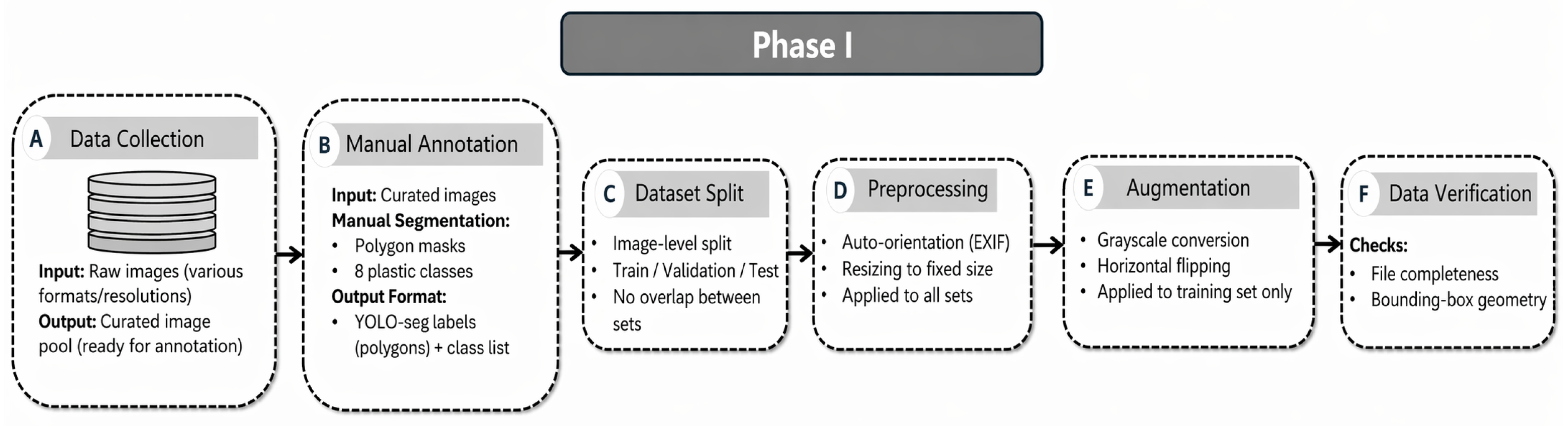
Phase I establishes the data pipeline used to transform heterogeneous image collections into a structured, facility-representative benchmark. This phase includes source aggregation, instance annotation, strict split isolation to prevent data leakage, standardized preprocessing, and training-set augmentation, as summarized in Figure 1.

3.1.1. Source Aggregation and Curation

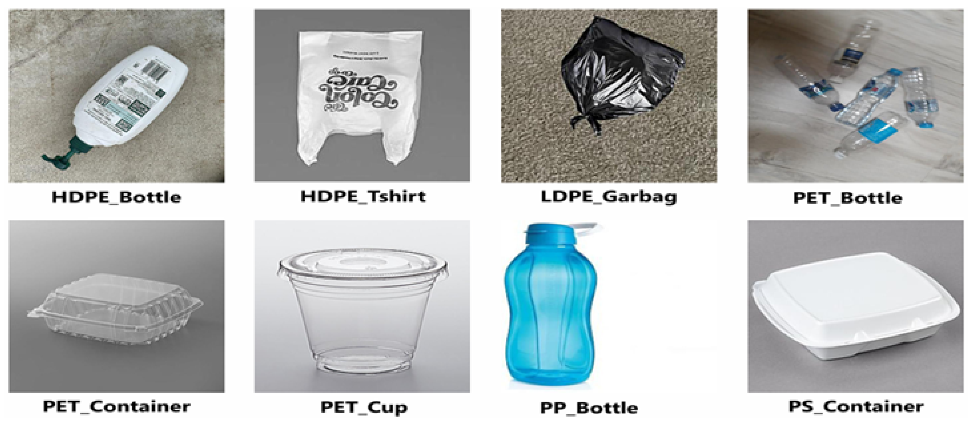
A total of 2486 images were collected from five publicly available sources: RealWaste from the UCI Machine Learning Repository [23], “Plastic Recyclable Detection” on Roboflow Universe (Roboflow Inc., Des Moines, IA, USA) [24], Alistair King’s “Recyclable and Household Waste Classification” dataset on Kaggle [25], Arkadiy Serezhkin’s “Drinking Waste Classification” dataset on Kaggle [26], and “Plastic Waste Detection” on Roboflow Universe [27]. Because these sources were originally prepared for image classification and/or bounding-box detection, all images were re-annotated to provide polygon-based instance masks for instance segmentation. The selected sources span variation in illumination, viewpoint, background clutter, and surface contamination, supporting evaluation under cross-source variability. This is important because dataset bias and domain shift can reduce model generalization when data are transferred across operating conditions [28]. The dataset covers common polymers in plastic waste streams, including PET, HDPE, LDPE, PP, and PS, consistent with resin identification practice [29]. Eight operational categories were defined: PET_Bottle, PET_Container, PET_Cup, HDPE_Bottle, HDPE_Tshirt_Bag, LDPE_Garbage, PP_Bottle_Container, and PS_Cup_Container, consistent with facility-oriented labeling choices in prior work [30]. Representative samples are shown in Figure 2. For standardization, all images were converted to JPEG (quality = 95) with chroma subsampling disabled (4:4:4), following the JPEG encoding specification to avoid subsampling artifacts and ensure consistent encoding across sources [31]. The standardized images were then organized into a unified directory structure for downstream processing.

3.1.2. Pixel-Level Instance Annotation

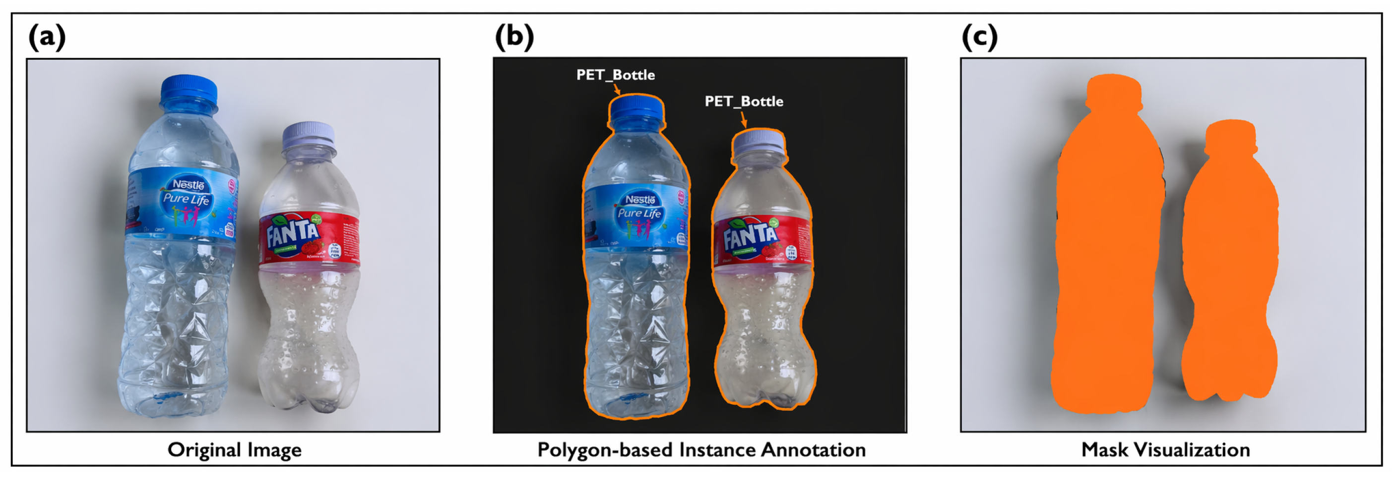
All 2486 curated images were imported into Roboflow, a web-based platform for dataset management and collaborative annotation workflows [32]. Instance-level annotation was then performed for plastic waste objects. For each visible object, the boundary was manually outlined using a polygon and assigned one of the eight predefined class labels. This process produced polygon-based instance masks suitable for training and evaluating instance segmentation models. All annotations were exported in COCO (Common Objects in Context) format [33]. In COCO, each instance is represented by its category label and associated geometry, including a bounding box and segmentation representation. Using this standardized format supports interoperability with widely used deep learning toolchains and established instance segmentation evaluation protocols. The resulting class distribution reflects the natural frequencies observed after curation. No resampling or class-balancing intervention was applied during dataset construction, in order to preserve the empirical class distribution and avoid introducing priors that may not hold under facility operating conditions. To visually illustrate the annotation workflow, a representative example is provided in Figure 3, showing the original image, the polygon-based instance annotation, and the corresponding mask visualization.

3.1.3. Strict Split Isolation and Leakage Prevention

Following annotation, the 2486 images were partitioned into three mutually exclusive subsets—training, validation, and test—using an image-level split. This ensures that each image appears in exactly one subset, preventing leakage of image-specific cues such as background patterns, viewpoint, or illumination conditions from training into evaluation. Such isolation supports an unbiased assessment of model generalization to unseen operating conditions. A 50%–15%–35% split allocation was adopted, as summarized in

Table 1. Dataset allocation across training, validation, and test subsets (before augmentation).

Dataset	No. of Images	Allocation
Training	1243	50%
Validation	373	15%
Test	870	35%
TOTAL	2486	100%

. The training subset (1243 images) was used for parameter learning, while the validation subset (373 images) supported model selection and performance monitoring during hyperparameter tuning. The test subset (870 images) was strictly held out for final evaluation.

3.1.4. Deterministic Preprocessing Pipeline

The same preprocessing pipeline was applied across the training, validation, and test splits. This included automatic EXIF-based orientation correction and resizing to a fixed $640\times 640$ resolution using Roboflow’s Stretch mode [34]. Applying identical preprocessing settings across all subsets avoids preprocessing-induced discrepancies and helps ensure that performance comparisons are not confounded by data-handling inconsistencies [35].

3.1.5. Training-Set Augmentation

Augmentation was applied exclusively to the training split using Roboflow’s augmentation suite [34]. Two transformations were used: grayscale conversion and horizontal flipping. These transformations were selected to increase appearance diversity in the training data and to reduce reliance on a single color or horizontal orientation pattern during learning. Grayscale conversion exposes the model to reduced color information under a consistent annotation setting, while horizontal flipping increases exposure to mirror-image variants [36]. After augmentation, the training set increased from 1243 to 1945 images, while the validation set (373 images) and test set (870 images) remained unchanged. As a result, the total curated dataset size reached 3188 images.

3.1.6. Automated Integrity Verification

To verify dataset integrity before model training, automated quality checks were performed on all 3188 annotation files. The validation protocol covered (i) file completeness and (ii) bounding-box geometry. Four files (≈0.1%) were flagged and excluded: two empty training annotation files and two problematic test files, including one empty file and one containing a degenerate bounding box with zero width. After filtering, the validated dataset comprised 3184 images with 4561 instances, distributed as shown in

Table 2. Waste material classification taxonomy showing class ID, material type, physical form, polymer number, and total object count.

Class ID	Class	Form	Polymer No.	Objects Count
0	HDPE	Bottle	2	638
1	HDPE	T-shirt Bag	2	513
2	LDPE	Garbage	4	477
3	PET	Bottle	1	726
4	PET	Container	1	425
5	PET	Cup	1	415
6	PP	Bottle/Container	5	697
7	PS	Cup/Container	6	670
TOTAL	–	–	–	4561

. The 99.9% pass rate indicates that annotation validity issues were rare. This validated dataset served as the basis for all subsequent experiments. Accordingly, the final validated test set comprised 868 images instead of the originally exported 870, due to integrity verification exclusions.

3.2. Phase II: Multi-Stage Optimization Model

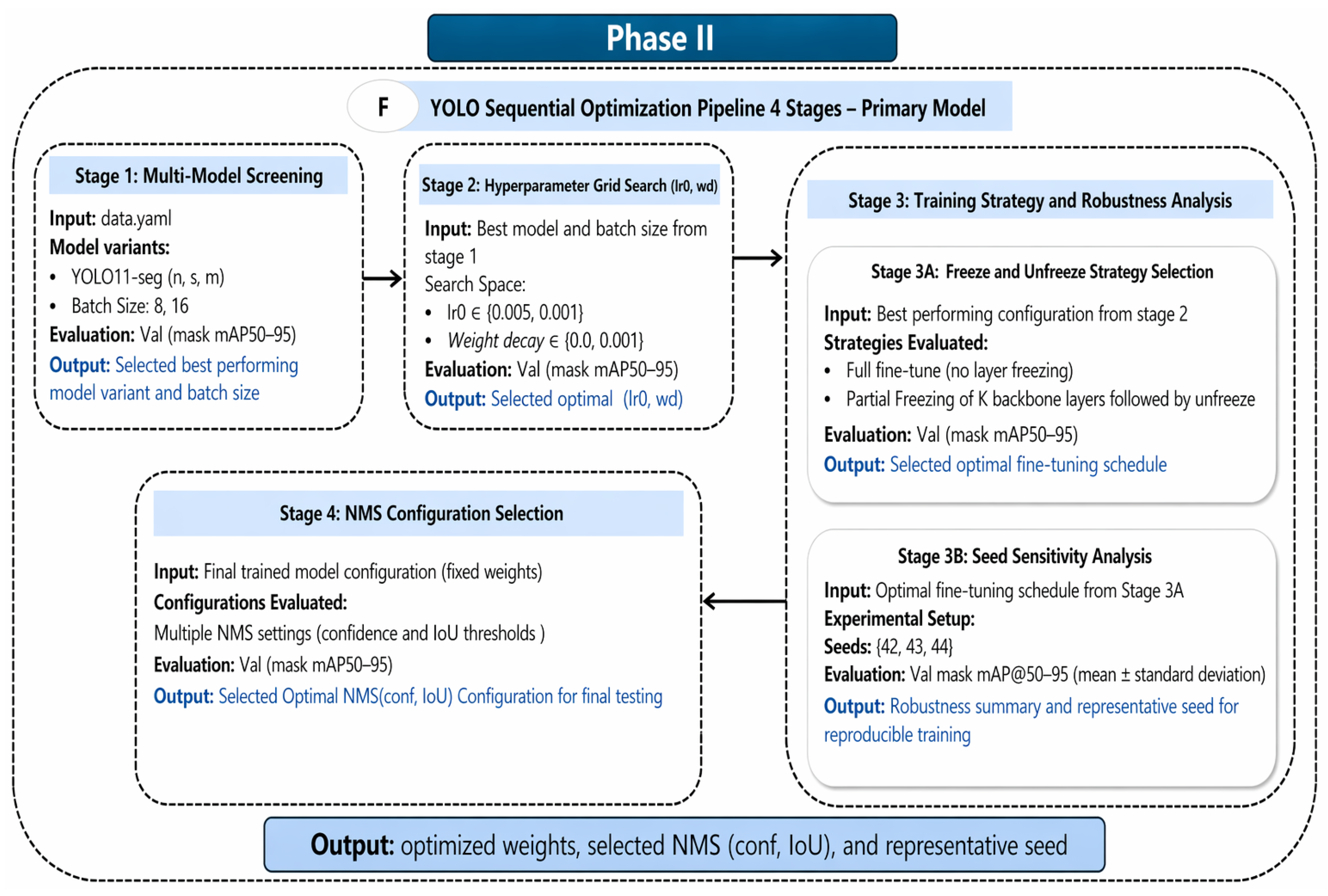
Phase II performs validation-driven model development and selection for the instance segmentation system through four stages: architecture and batch-size screening, hyperparameter search, training strategy and robustness analysis, and NMS selection. Across all YOLOv11 stages, training was conducted within the official Ultralytics framework using standard SGD-based optimization with momentum 0.9. Unless otherwise stated for a given stage, the default training schedule of the framework was retained, and runs were terminated early when validation performance did not improve for 10 consecutive epochs (patience = 10). The staged epoch budgets (30, 50, 75, and 100 epochs) were chosen progressively to match the purpose of each stage: low-cost screening in Stage 1, moderate hyperparameter refinement in Stage 2, deeper comparison of transfer learning schedules in Stage 3A, and more stable robustness assessment across independent seeds in Stage 3B. The workflow is illustrated in Figure 4, and the complete optimization procedure is summarized in Algorithm 1.

Algorithm 1 Multi-Stage Hyperparameter and Architecture Optimization

INPUT: Dataset splits $(D_{train},D_{val})$, pretrained weights OUTPUT: Optimized model ${\theta }^{*}$, NMS configuration $nm{s}^{*}$   1: Load dataset splits $(D_{train},D_{val})$   2: Stage 1: Architecture and batch size screening   3: for each model $y\in${YOLOv11n-seg, YOLOv11s-seg, YOLOv11m-seg} do   4:    for each batch size $b\in \{8,16\}$ do   5:       Train for 30 epochs $(l{r}_0=0.01,\lambda =0.0005,patience=10)$   6:       Evaluate mask $mAP@50:95$ on $D_{val}$   7:       Record efficiency metrics (params, size, latency)   8:    end for   9: end for 10: Select $(y^{*},b^{*})$ with highest mask $mAP@50:95$ 11: Stage 2: Hyperparameter grid search 12: for each $l{r}_0\in \{0.005,0.001\}$ do 13:    for each $\lambda \in \{0.0,0.001\}$ do 14:       Train $(y^{*},b^{*})$ for 50 epochs $(patience=10)$ 15:       Evaluate mask $mAP@50:95$ on $D_{val}$ 16:    end for 17: end for 18: Select $(l{r}_0^{*},{\lambda }^{*})$ with highest mask $mAP@50:95$ 19: Stage 3A: Freeze strategy ablation 20: for each strategy $s\in${none, freeze-10→unfreeze, freeze-12→unfreeze} do 21:    Train $(y^{*},b^{*},l{r}_0^{*},{\lambda }^{*})$ for 75 epochs $(patience=10)$ 22:    Evaluate mask $mAP@50:95$ on $D_{val}$; record precision/recall/F1 23: end for 24: Select $s^{*}$ with highest mask $mAP@50:95$ 25: Stage 3B: Extended training with seed robustness 26: for each seed $e\in \{42,43,44\}$ do 27:    Train $(y^{*},b^{*},l{r}_0^{*},{\lambda }^{*},s^{*})$ for 100 epochs $(patience=10)$ 28:    Evaluate mask $mAP@50:95$ on $D_{val}$ 29: end for 30: Compute ${\mu }_{mAP}$, ${\sigma }_{mAP}$, and CV across seeds 31: Fix seed $=42$ for subsequent stages $\to {\theta }^{*}$ 32: Stage 4: NMS threshold optimization 33: for each NMS configuration $n\in \{A,B,C\}$ do 34:    Evaluate ${\theta }^{*}$ on $D_{val}$ using $n.conf$ and $n.iou$ 35:    Record mask $mAP@50:95$, precision, recall, F1 36: end for 37: Select $nm{s}^{*}$ with highest mask $mAP@50:95$ 38: Return${\theta }^{*},nm{s}^{*}$

The segmentation experiments in this study used the official Ultralytics YOLOv11 instance segmentation implementation [37] without custom architectural modification to the backbone, neck, or segmentation head. YOLOv11 was selected as a contemporary single-stage segmentation family with practical accuracy–efficiency characteristics and official implementation support, making it suitable for high-throughput waste-scene analysis. Its use in this study does not imply an a priori assumption of optimality; rather, its suitability was assessed empirically through controlled architecture screening within the YOLOv11 family and through comparative evaluation against representative baselines under matched experimental conditions. This study does not introduce a new optimizer or optimization algorithm. Rather, the staged YOLOv11 development procedure is implemented within the official Ultralytics training framework, using standard SGD-based optimization throughout.

3.2.1. Stage 1: Architecture and Batch-Size Screening

Three official YOLOv11 segmentation variants (YOLOv11n-seg, YOLOv11s-seg, and YOLOv11m-seg) were evaluated with batch sizes 8 and 16 under a common baseline protocol (30 epochs, SGD, $l{r}_0=0.01$, $\lambda =0.0005$, patience = 10). This stage was designed to assess the suitability of different model capacities within the same YOLOv11 family under controlled conditions, rather than to assume that a specific variant was optimal a priori. Selection was based on validation mask mAP@50:95. YOLOv11s-seg with batch size 16 achieved the highest performance (0.9205) with favorable efficiency (10.11 M parameters, 38.58 MB, 150.86 ms/image under single-image inference on an NVIDIA A100 GPU) and was selected for subsequent stages. No custom architectural modifications were made to the backbone, neck, or segmentation head of any evaluated variant.

3.2.2. Stage 2: Hyperparameter Search

Following the Stage 1 model and batch-size screening, a constrained $2\times 2$ hyperparameter search was performed on the selected YOLOv11s-seg configuration to refine the two directly optimized training variables: the initial learning rate ($lr0\in \{0.005,0.001\}$) and weight decay ($\lambda \in \{0.0,0.001\}$). Each configuration was trained for up to 50 epochs with patience = 10, and selection was based on validation mask mAP@50:95. This stage was intentionally designed as a focused refinement step rather than an exhaustive hyperparameter optimization study. The goal was to preserve a controlled and computationally tractable selection protocol after Stage 1 had already fixed the model variant and batch size. Under this design, the search targeted two directly optimized training variables so that performance differences could be interpreted more clearly at this stage. The optimal Stage 2 configuration was $lr0=0.001$ and $\lambda =0.0$, which was then advanced to Stage 3. Throughout these stages, the underlying training optimizer remained the standard SGD-based optimizer of the official YOLOv11 training pipeline; only the selected training variables and stage-specific evaluation settings were varied.

3.2.3. Stage 3: Training Strategy and Robustness

3A: Freeze–Unfreeze Ablation

Three transfer learning schedules were compared over 75 epochs with patience = 10: full fine-tuning, freeze-10→unfreeze, and freeze-12→unfreeze. The freeze-12 schedule achieved the highest validation mask mAP@50:95 and was selected.

3B: Seed Robustness

The Stage 3A winner was retrained across seeds {42, 43, 44} for 100 epochs. Variability was assessed using the mean, standard deviation, and coefficient of variation of validation mask mAP@50:95. Seed 42 was fixed for subsequent stages for reproducibility.

3.2.4. Stage 4: NMS Optimization

Three NMS configurations were evaluated on the Stage 3B model without further training: The NMS search was intentionally restricted to a compact validation-time grid over two practically important parameters: confidence threshold $\in \{0.25,0.50\}$ and IoU threshold $\in \{0.50,0.70\}$. Rather than performing a broad continuous search, we selected three representative operating points to compare more permissive versus more selective suppression behavior under a controlled and reproducible validation protocol.

(A)

conf = 0.25, IoU = 0.50

(B)

conf = 0.25, IoU = 0.70

(C)

conf = 0.50, IoU = 0.50

Configuration (A) maximized validation mask mAP@50:95 and was locked for final evaluation.

3.2.5. Baseline Comparison

The optimized YOLOv11s-seg model [37] was compared against YOLOv8s-seg [38], Mask R-CNN with a ResNet-50-FPN backbone [14,39,40], and the more recent transformer-based RF-DETR-Seg (Small) [41,42] using the same fixed train/validation/test split and the finalized evaluation protocol. All models were evaluated with the COCO protocol [33] on the locked held-out test set after optimization. Since the compared methods belong to different architectural families and training frameworks, the comparison was not intended to force identical implementation structure across all baselines. Instead, each model was trained and evaluated under framework-appropriate settings while preserving the same dataset split, locked held-out test set, and COCO-style evaluation protocol, so that the comparison reflects practically relevant performance differences between representative one-stage, two-stage, and transformer-based instance segmentation pipelines.

The staged design in Algorithm 1 intentionally allocates increasing training budgets as the search space narrows. Early stages are used for economical elimination of clearly suboptimal configurations, whereas later stages devote more epochs to fewer candidate settings in order to reduce variance in validation-based comparison and to support more reliable selection of transfer learning schedules and seed-robust configurations.

3.3. Phase III: Evaluation and Downstream Inference

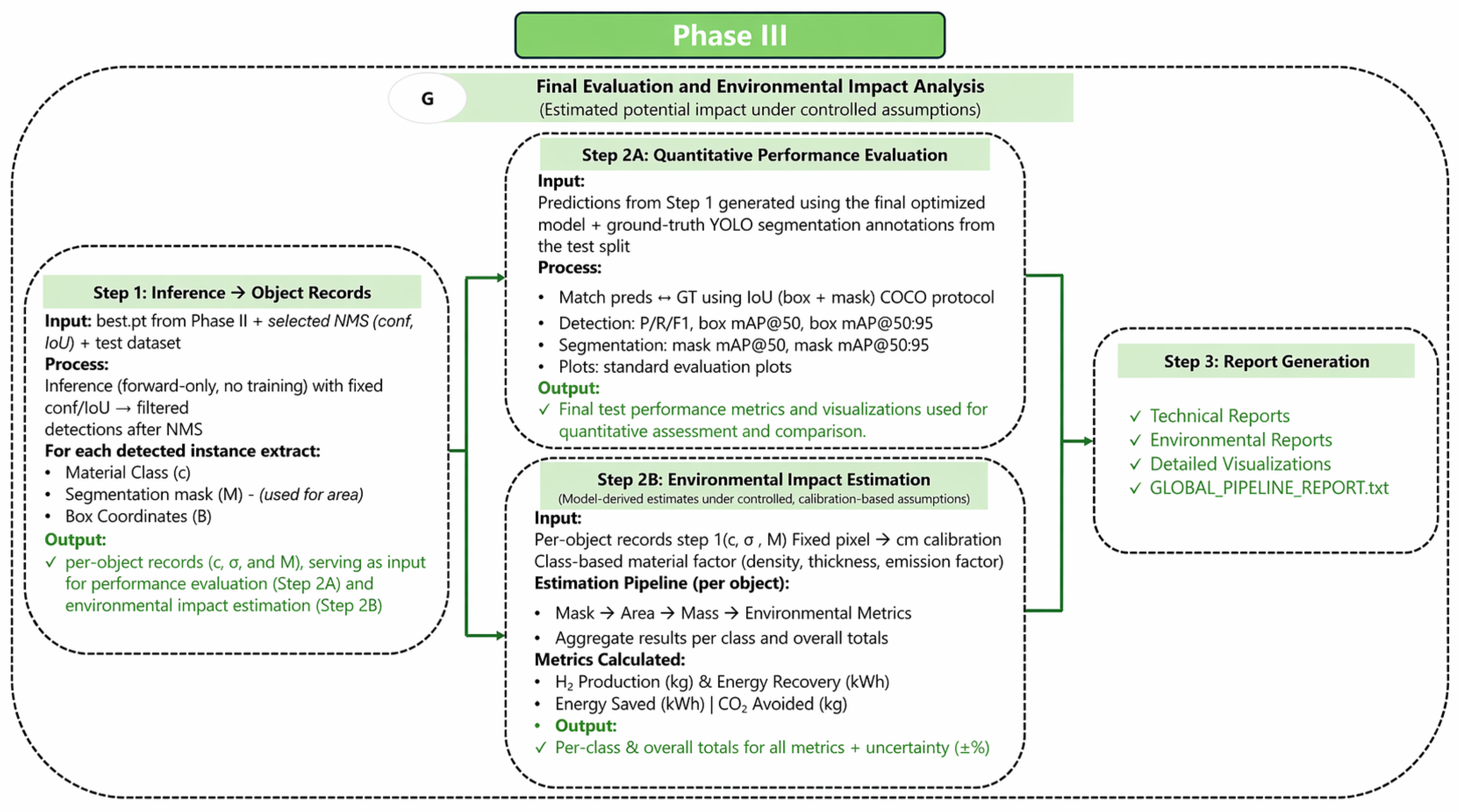
Phase III applies the optimized model to the held-out test set and translates segmentation outputs into downstream environmental indicators. The workflow includes inference, COCO-based spatial evaluation, and scenario-based impact estimation, as illustrated in Figure 5.

3.3.1. Step 1: Inference and Object Extraction

The final optimized model from Phase II was applied to the held-out test set in inference-only mode, with no additional training or tuning. Inference was performed on 868 test images using the finalized YOLOv11s-seg configuration and the selected Stage 1–4 settings, including the fixed NMS thresholds (confidence $=0.25$, IoU $=0.50$). For each detected object, the predicted class $c\in \{0,\dots ,7\}$, segmentation mask M, and bounding box $B=(x_{min},y_{min},x_{max},y_{max})$ were extracted and stored.

These outputs served as inputs to Step 2A for COCO-based spatial evaluation and to Step 2B for mask-to-mass estimation and downstream environmental analysis.

3.3.2. Step 2A: COCO-Based Spatial Evaluation

Predictions on the held-out test set were evaluated against manually annotated ground truth labels using the COCO instance segmentation protocol [33]. A prediction was counted as correct only when the class label matched and the predicted mask satisfied the required Intersection-over-Union (IoU) threshold with the ground truth. Unmatched predictions were treated as false positives, and unmatched ground truth objects as false negatives. Performance was assessed using precision, recall, F1-score, mask mAP@50, and mask mAP@50:95, with mask mAP@50:95 used as the primary metric because it reflects the standard COCO criterion and provides a stricter measure of mask quality. These metrics jointly capture detection, classification, and segmentation performance. Accurate mask localization is especially important because all downstream estimates are derived from predicted object areas.

3.3.3. Step 2B: Physics-Informed Mass Mapping

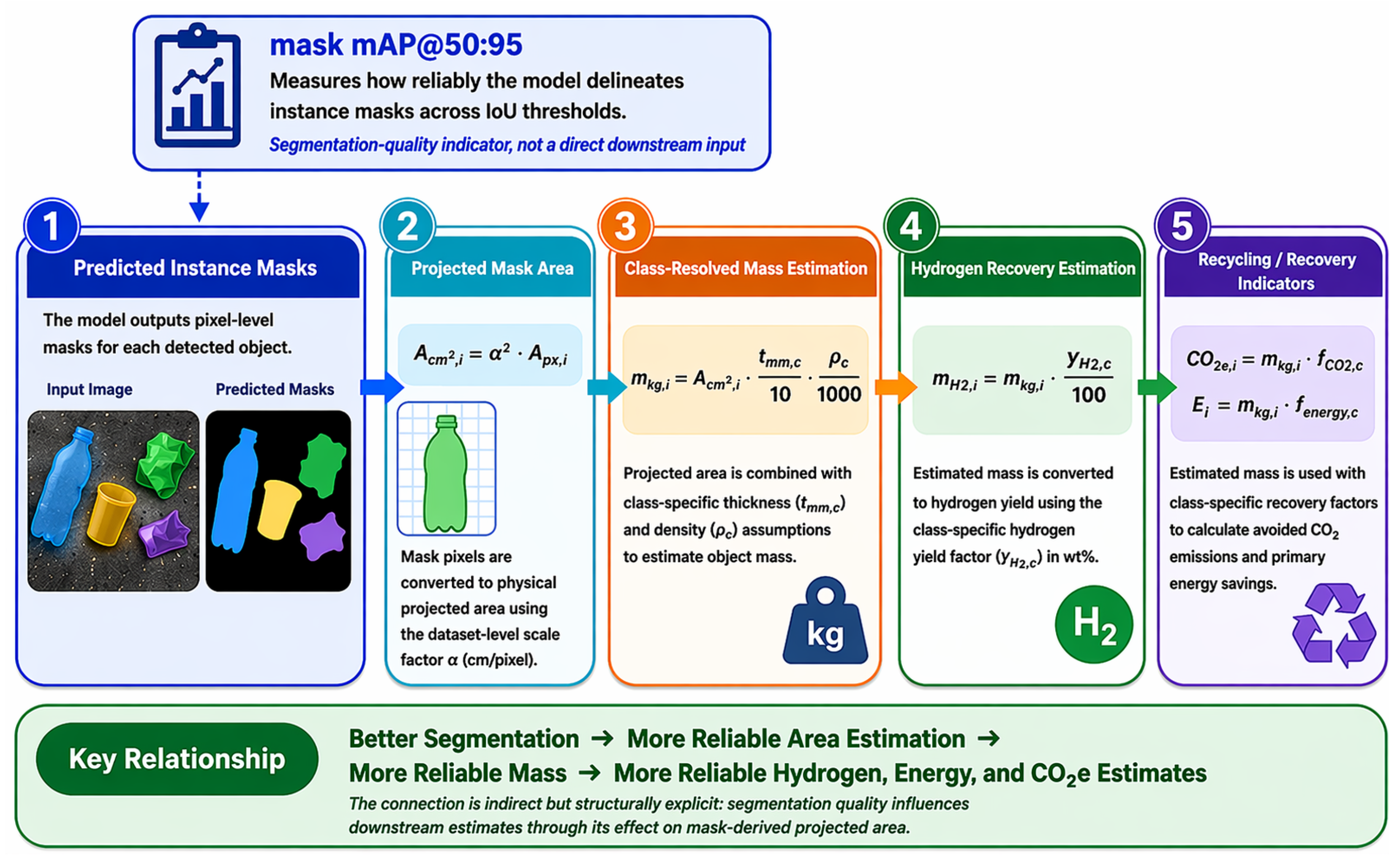
The proposed system converts segmentation output into object-level mass and downstream recovery indicators through a sequential estimation chain. For each detected instance, the predicted segmentation mask first provides the projected object area in pixels. Using the adopted dataset-level scale factor, this projected area is converted into physical area in cm². The resulting area is then combined with class-specific thickness and density assumptions to estimate object mass. These mass estimates are subsequently used as the common input to the downstream hydrogen-yield, avoided CO₂e-emissions, and primary-energy calculations. Accordingly, the downstream indicators are not computed directly from segmentation metrics themselves, but from mass estimates derived from segmentation-based geometric information. This object-level conversion chain is summarized in Figure 6. Step 2B converts predicted masks into downstream quantitative indicators under two reporting pathways: Scenario A (material recycling) and Scenario B (waste-to-energy through hydrogen recovery). In this framework, the connection between perception and quantification is direct: the predicted instance masks provide the projected object geometry from which object-wise area is computed, and this segmentation-derived area is then propagated through the analytical mass-estimation model. Rather than applying an empirical black-box regression, this module uses an explicit physics-informed analytical formulation that combines mask-derived geometry with class-specific material properties and literature-based conversion factors to estimate mass, hydrogen potential, energy, and CO₂-related indicators. Representative polymer properties follow established standards [43,44,45,46,47,48,49], while recycling and hydrogen factors are drawn from published LCI datasets and conversion studies [50,51,52,53,54,55].

The two pathways are reported separately to avoid double-counting. Both use the same mass estimates from Equations (1)–(3), differ only in the assumed end-of-life treatment, and are interpreted with the uncertainty model defined below.

Notation Summary

In the following equations, index i denotes an individual detected object and index c denotes its assigned plastic class. $A_{\mathrm{px},i}$ is the foreground mask area in pixels, $A_{{\mathrm{cm}}^2,i}$ is the corresponding estimated projected physical area in cm², and $\alpha$ is the dataset-level linear scale factor in cm/pixel. The quantity $t_{\mathrm{mm},c}$ denotes the class-specific wall thickness in mm, ${\rho }_c$ denotes the class-specific material density in g/cm³, and $V_{{\mathrm{cm}}^3,i}$ denotes the estimated material volume in cm³. The resulting object mass is denoted by $m_{\mathrm{kg},i}$ in kg. For downstream calculations, $f_{{\mathrm{CO}}_2,c}$ and $f_{\mathrm{energy},c}$ denote the class-specific recycling factors for CO₂ avoidance and primary energy savings, respectively, while $y_{{\mathrm{H}}_2,c}$ denotes the class-specific hydrogen yield in wt%. At the aggregate level, N denotes the total number of detected objects used in the summation formulas, and $f_{\mathrm{uncertainty}}$ denotes the assigned relative uncertainty factor used in the scenario-based uncertainty analysis.

Pixel-to-Mass Mapping

The first step in the estimation pipeline transforms pixel-level instance masks into estimated physical area through an explicit geometric area-mapping procedure. For each detected object i, the projected planar area is computed by counting the foreground pixels, denoted as $A_{\mathrm{px},i}$, within its segmentation mask. A global linear scaling factor $\alpha$ (set to $0.05$ cm/pixel in this study) is then used as a dataset-level geometric calibration parameter to convert pixel area into estimated physical area $A_{{\mathrm{cm}}^2,i}$:

$$A_{{\mathrm{cm}}^2,i}=A_{\mathrm{px},i}{\alpha }^2$$

(1)

where $\alpha$ is a nominal scale factor ($\alpha =0.05$ cm/pixel), corresponding to a representative field of view of approximately $32\times 32$ cm for a $640\times 640$-pixel image under close-range waste-scene imaging conditions. In this formulation, $\alpha$ serves as an explicit dataset-level calibration assumption that enables physically interpretable area estimation across heterogeneous imagery. Because the dataset aggregates images from multiple sources with varying acquisition conditions, $\alpha$ is applied uniformly as a fixed approximation for comparative batch-level analysis, and per-image geometric calibration was not performed. Accordingly, the resulting mass estimates are interpreted as stream-level order-of-magnitude indicators rather than precise gravimetric measurements. No object-level or batch-level gravimetric ground truth measurements were available for the present dataset; therefore, the absolute accuracy of the estimated masses could not be directly validated in this study.

Volumetric Mass Estimation

To translate the projected 2D area into mass $m_{\mathrm{kg},i}$, the model adopts a physics-informed sheet-equivalent volumetric formulation. Under this formulation, each detected plastic object is represented as a class-conditioned planar material layer defined by its projected area and a characteristic wall thickness, enabling mass estimation when object-level three-dimensional reconstruction is not available. For each detected class c, material properties—density ${\rho }_c$ (g/cm³) and wall thickness $t_{\mathrm{mm},c}$ (mm)—are assigned using the standardized material database summarized in

Table 3. Standardized physical properties assigned to detected plastic waste classes for environmental impact estimation (Data derived from ISO/ASTM specifications and polymer reference data [43,44,45,46,47,48,49]).

Class ID	Density $\mathit{\rho }$ (g/cm3)	Thickness t (mm)
		Min	Nominal	Max
HDPE_Bottle	0.96	0.50	0.80	1.20
HDPE_Tshirt_Bag	0.95	0.03	0.06	0.10
LDPE_Garbage	0.92	0.04	0.08	0.12
PET_Bottle	1.38	0.30	0.40	0.50
PET_Container	1.38	0.40	0.60	0.80
PET_Cup	1.37	0.25	0.30	0.35
PP_Bottle_Container	0.91	0.80	1.20	1.50
PS_Cup_Container	1.05	1.00	1.50	2.00

. These parameters are grounded in internationally recognized ISO and ASTM polymer specifications and reference data [43,44,45,46,47,48,49]. To reflect manufacturing variability commonly observed in plastic waste streams, the database defines minimum, nominal, and maximum thickness scenarios. Unless otherwise stated, the nominal value is used for baseline calculations.

The polymer material volume $V_{{\mathrm{cm}}^3,i}$ is then estimated through an explicit geometric extrusion of the projected area $A_{{\mathrm{cm}}^2,i}$ using the class-specific wall thickness:

$$V_{{\mathrm{cm}}^3,i}=A_{{\mathrm{cm}}^2,i}·\left({\displaystyle \frac{t_{\mathrm{mm},c}}{10}}\right)$$

(2)

where $t_{\mathrm{mm},c}$ is the class-specific wall thickness in millimeters, and division by 10 converts thickness from millimeters to centimeters.

The object mass is then computed deterministically from the estimated material volume and class-specific density, and normalized to kilograms to serve as the functional unit for Life Cycle Assessment (LCA):

$$m_{\mathrm{kg},i}={\displaystyle \frac{V_{{\mathrm{cm}}^3,i}·{\rho }_c}{1000}}$$

(3)

Together, Equations (1)–(3) define an explicit class-conditioned mapping from segmentation-derived geometry to estimated material mass under stated geometric and material assumptions, providing a physically interpretable basis for stream-level quantification. Under this formulation, the quality of instance-mask delineation directly influences the estimated projected area and therefore propagates into the downstream mass estimate. This calculation targets the polymer mass rather than the internal void capacity of a container. Although real waste items exhibit complex three-dimensional geometries, the sheet-equivalent approximation provides a calibrated and internally consistent mass estimate suitable for comparative batch-level assessment.

Scenario A: Material Recycling

In the material recycling scenario, the study quantifies potential CO₂ avoidance and primary energy savings under a resin substitution assumption using class-specific factors from resin LCI datasets [50,51,52,53,54]:

$$E_{{\mathrm{CO}}_2\text{-}\mathrm{saved},i}=m_{\mathrm{kg},i}\times f_{{\mathrm{CO}}_2,c}$$

(4)

$$E_{\mathrm{saved},\mathrm{MJ},i}=m_{\mathrm{kg},i}\times f_{\mathrm{energy},c}$$

(5)

$$E_{\mathrm{saved},\mathrm{kWh},i}={\displaystyle \frac{E_{\mathrm{saved},\mathrm{MJ},i}}{3.6}}$$

(6)

These indicators are reported only for the recycling pathway and are distinct from the energy-recovery metrics, ensuring that benefits are not double-counted for the same plastic mass.

Scenario B: Waste-to-Energy

Under the waste-to-energy pathway, hydrogen yield and associated energy are computed as:

$$H_{2,\mathrm{kg},i}=m_{\mathrm{kg},i}\left({\displaystyle \frac{y_{H_2,c}}{100}}\right)$$

(7)

$$E_{\mathrm{MJ},i}=H_{2,\mathrm{kg},i}\times 120$$

(8)

$$E_{\mathrm{kWh},i}={\displaystyle \frac{E_{\mathrm{MJ},i}}{3.6}}$$

(9)

The two pathways are reported separately to avoid double-counting.

Dataset-Level Aggregation

Dataset-level totals are computed by summing object-level estimates across all detected objects:

$$M_{\mathrm{total}}=\sum _{i=1}^N{m}_{\mathrm{kg},i}$$

(10)

$$H_{2,\mathrm{total}}=\sum _{i=1}^N{H}_{2,\mathrm{kg},i}$$

(11)

$$E_{{\mathrm{H}}_2,\mathrm{total}}=\sum _{i=1}^N{E}_{\mathrm{kWh},i}$$

(12)

$$E_{{\mathrm{CO}}_2\text{-}\mathrm{saved},\mathrm{total}}=\sum _{i=1}^N{E}_{{\mathrm{CO}}_2\text{-}\mathrm{saved},i}$$

(13)

$$E_{\mathrm{saved},\mathrm{total}}=\sum _{i=1}^N{E}_{\mathrm{saved},\mathrm{kWh},i}$$

(14)

These aggregations support both per-class analysis and overall dataset-level summaries. The recycling indicators for CO₂ avoidance and primary energy savings (Equations (13) and (14)) and the hydrogen recovery indicators (Equations (11) and (12)) represent alternative fates for the same plastic mass and are therefore reported in parallel rather than combined into a single total-benefit metric.

Scenario-Based Uncertainty Analysis

Because the proposed workflow estimates physical and valorization-related quantities from heterogeneous 2D images rather than direct laboratory measurements, uncertainty was treated as a scenario-based indicative range rather than a strict metrological confidence interval. The reported bounds reflect the dominant practical sources of variation in the downstream calculations, including image-scale approximation, segmentation-derived size estimation, nominal material-property assignment, and literature-based conversion factors.

The conversion from segmented pixel area to physical area was performed using a fixed scale factor of $\alpha =0.05$ cm/pixel. In this study, this factor was used as a nominal dataset-level geometric approximation rather than an image-specific empirical calibration parameter. Because the dataset aggregates images from heterogeneous sources with potentially different acquisition distances and viewing conditions, this simplification introduces uncertainty in the absolute physical scale of the derived mass estimates. Accordingly, the downstream mass, hydrogen potential, and CO₂e estimates reported in this work should be interpreted as indicative scenario-based quantities rather than precision-grade physical measurements.

Because part of the uncertainty originates from dataset-level scale approximation rather than symmetric random measurement noise, the reported uncertainty ranges should be interpreted as indicative sensitivity bounds for transparent stream-level reporting, not as directionally resolved physical error distributions or formal statistical confidence intervals. In particular, an overestimated scale factor would tend to inflate the derived mass and CO₂e estimates, whereas an underestimated factor would tend to reduce them.

The selected ranges were applied to the derived stream-level outputs after locked test-set inference and are intended to indicate sensitivity to the main simplifying assumptions of the pipeline rather than formal statistical confidence from repeated measurements.

For a calculated quantity X, the associated uncertainty is estimated as:

$${\sigma }_X=X\times f_{\mathrm{uncertainty}}$$

(15)

where X denotes the downstream quantity of interest (e.g., total mass, hydrogen yield, energy, or CO₂e avoidance), ${\sigma }_X$ denotes the corresponding absolute scenario-based uncertainty bound, and $f_{\mathrm{uncertainty}}$ denotes the assigned relative uncertainty factor for that quantity. In this study, a $\pm 7\%$ range was used for total estimated mass, reflecting the expected effect of image-scale and size-approximation uncertainty on volumetric inference. Hydrogen yield was reported with a $\pm 10\%$ range to account for additional conversion uncertainty. Energy potential was assigned a $\pm 8\%$ range, while avoided CO₂ emissions were assigned a $\pm 12\%$ range to reflect the cumulative sensitivity of offset assumptions. The selected ranges are study-level assumptions introduced for transparent interpretation of stream-level estimates and are not presented as direct prescribed values from ISO 14040/14044 or the cited review literature. This framing is consistent with broader life-cycle-based reporting principles related to data quality, system boundaries, and transparency [56,57,58]. Results are therefore reported as $X\pm {\sigma }_X$ and should be interpreted as indicative stream-level bounds under the study assumptions rather than strict propagated measurement errors or formal statistical confidence intervals.

Segmentation Quality and Downstream Sensitivity

All downstream indicators in this study originate from projected object area obtained from pixel-level segmentation (Equations (1)–(14)). Accordingly, the connection between segmentation quality and downstream hydrogen recovery or recycling substitution estimates is indirect but structurally explicit. The mask mAP@50:95 reported in Step 2A is not itself used as an input parameter in the downstream equations; rather, it serves as a segmentation-quality indicator of how reliably the model delineates instance masks across IoU thresholds. These masks determine the projected area term in Equation (1), which then propagates through the geometric and material assumptions of Equations (2) and (3) to produce class-resolved mass estimates. The resulting mass terms are then used in the downstream hydrogen recovery, energy, and recycling substitution calculations (Equations (4)–(14)). Under this formulation, improved segmentation quality supports more reliable area estimation, which in turn supports more stable mass-based downstream indicators. Because object mass scales linearly with area (Equation (3)) and the downstream indicators scale linearly with mass, segmentation-related deviations can influence the final stream-level estimates approximately linearly. For this reason, mask mAP@50:95 is interpreted here as a perception-quality indicator that supports the credibility of the downstream analysis, rather than as a direct physical or process-engineering variable. Figure 6 summarizes this relationship and illustrates how segmentation quality supports the downstream hydrogen recovery and recycling substitution estimates through mask-derived projected area and class-resolved mass estimation.

As illustrated in Figure 6, the downstream quantities are derived from segmentation-based geometric information through the sequential object-level estimation chain defined in Equations (1)–(14), rather than from the segmentation metric itself.

4. Results and Discussion

4.1. Experimental Setup and Computational Environment

All experiments were conducted in the Google Colaboratory Pro environment (Google LLC, Mountain View, CA, USA) using an NVIDIA A100 Tensor Core GPU under a CUDA-enabled runtime. The software environment included Python 3.12 (Python Software Foundation, Wilmington, DE, USA), PyTorch 2.9.0+cu126, Torchvision 0.24.0+cu126, the Ultralytics framework (version 8.4.14), OpenCV 4.13.0, NumPy 2.0.2, Pandas 2.2.2, and pycocotools for COCO-style evaluation. The YOLOv11 experiments were implemented using the official Ultralytics instance segmentation framework configuration, with no custom architectural changes introduced to the backbone, neck, or segmentation head. To support reproducibility, the software environment was fixed at the beginning of the experimental campaign. A uniform preprocessing pipeline was applied across all dataset splits using Roboflow’s automated tools, including EXIF-based orientation correction and resizing to $640\times 640$ pixels using a fixed stretch-based setting. Although this choice may introduce aspect-ratio distortion for some objects, it was applied consistently across all dataset splits and compared models to preserve a controlled and reproducible evaluation protocol.

4.2. Phase II: Multi-Stage Optimization Results

4.2.1. Stage 1 Results: Architecture Screening and Efficiency

Stage 1 evaluated six training configurations by pairing three YOLOv11-seg variants (nano, small, and medium) with two batch sizes (8 and 16). All runs used the same baseline protocol (image size 640, SGD with momentum 0.9, initial learning rate 0.01, weight decay 0.0005, seed 42) and were trained for up to 30 epochs with early stopping (patience = 10), providing a low-cost screening stage before deeper tuning. The full comparison is reported in

Table 4. Stage 1 multi-model screening results: validation performance across three YOLOv11-seg variants and two batch sizes.

Model	Batch	Params (M)	Size (MB)	Inf. (ms)	mAP@50:95
YOLOv11m-seg	8	22.421	85.53	393.71	0.9117
	16	22.421	85.53	408.87	0.9122
YOLOv11n-seg	8	2.877	10.97	445.83	0.8964
	16	2.877	10.97	83.26	0.9050
YOLOv11s-seg	8	10.11	38.58	262.48	0.9139
	16	10.11	38.58	150.86	0.9205

.

Table 4 shows that increasing batch size from 8 to 16 produced consistent gains in validation mask mAP@50:95 for the nano and small variants, while the medium variant changed only marginally (nano: $+0.0086$; small: $+0.0066$; medium: $+0.0005$ in absolute mAP). These results indicate that batch size influenced convergence under a fixed training budget, although the effect was architecture-dependent. Model size also did not translate monotonically into better accuracy: despite its larger capacity, YOLOv11m-seg did not outperform the small variant under the same protocol. Based on the primary selection criterion, YOLOv11s-seg with batch size 16 was selected, achieving validation mask mAP@50:95 = 0.9205 with 10.11M parameters, 38.58 MB weights, and 150.86 ms/image under single-image inference on an NVIDIA A100 GPU.

4.2.2. Stage 2 Results: Hyperparameter Search

Table 5. Stage 2 hyperparameter grid search: validation performance across learning rate $l{r}_0$ and weight decay $\lambda$ combinations.

Learning Rate (${\mathit{lr}}_0$)	Weight Decay ($\mathit{\lambda }$)	Val Time (s)	Mask mAP@50:95
0.005	0.0000	10.64	0.9162
0.005	0.0010	10.49	0.9229
0.001	0.0000	10.59	0.9324
0.001	0.0010	10.97	0.9290

reports the results of the $2\times 2$ grid over $l{r}_0\in \{0.005,0.001\}$ and $\lambda \in \{0.0,0.001\}$ for the selected YOLOv11s-seg configuration (batch size 16). Validation performance was assessed primarily using mask mAP@50:95.

Across the evaluated settings, the learning rate had the largest effect. The best-performing configuration at $l{r}_0=0.001$ achieved 0.9324, compared with 0.9229 for the best configuration at $l{r}_0=0.005$, corresponding to an absolute improvement of $+0.0095$ in mask mAP@50:95. Weight decay showed a regime-dependent effect: at $l{r}_0=0.005$, adding $\lambda =0.001$ improved performance from 0.9162 to 0.9229 ($\mathrm{\Delta }=+0.0067$), whereas at $l{r}_0=0.001$, it reduced performance from 0.9324 to 0.9290 ($\mathrm{\Delta }=-0.0034$). The selected Stage 2 configuration was therefore $l{r}_0=0.001$ and $\lambda =0.0$.

4.2.3. Stage 3A Results: Transfer Learning Schedule Ablation

Table 6. Stage 3A backbone freezing strategy comparison.

Metric	No Freeze	Freeze-10	Freeze-12
Frozen Layers	0	10	12
$l{r}_0$	0.001	0.001	0.001
$\lambda$	0.0	0.0	0.0
F1-Score	0.9309	0.9300	0.9371
Mask mAP@50:95	0.9337	0.9335	0.9395

summarizes validation results for the three freezing strategies under identical training settings (seed = 42, up to 75 epochs, patience = 10). The freeze-12-then-unfreeze training schedule achieved the best validation performance (mask mAP@50:95 = 0.9395; F1-score = 0.9371) and was selected for subsequent stages.

Relative to the no-freeze baseline (0.9337), the selected schedule produced an absolute gain of $+0.0058$ in mask mAP@50:95. In contrast, the freeze-10 then unfreeze setting showed no meaningful change (0.9335 vs. 0.9337; $\mathrm{\Delta }=-0.0002$). These results indicate that stronger initial freezing provided a modest but consistent validation benefit under the same architecture and hyperparameter setting.

4.2.4. Stage 3B Results: Random Seed Robustness

To verify that performance was not dependent on a favorable initialization, the optimized configuration (YOLOv11s-seg, $l{r}_0=0.001$, $\lambda =0.0$, freeze-12 schedule) was retrained with three independent seeds (42, 43, and 44). As shown in

Table 7. Stage 3B random seed robustness analysis: validation performance across three independent training runs with different seeds.

Seed	Val F1	Val Mask mAP@50:95
42	0.9334	0.9365
43	0.9156	0.9322
44	0.9335	0.9304
Mean ($\mu$)	0.9275	0.9330
Std ($\sigma$)	0.0103	0.0032
CV (%)	1.11%	0.34%

, validation mask mAP@50:95 remained stable across runs (0.9365, 0.9322, and 0.9304), yielding a mean of 0.9330 with a low coefficient of variation ($\mathrm{CV}=0.34\%$). In contrast, the F1-score showed slightly higher sensitivity ($\mathrm{CV}=1.11\%$), ranging from 0.9156 to 0.9335.

These results show that, although the precision–recall balance varied slightly across initializations, mask quality remained consistently stable. This supports the robustness of the training procedure to stochastic initialization. For consistency with earlier stages, seed 42 was retained for final evaluation and subsequent analyses.

4.2.5. Stage 4 Results: NMS Calibration

With the training configuration fixed through Stages 1–3B, Stage 4 optimized inference-time NMS parameters. The Stage 3B model (seed 42) was evaluated on the validation set using three NMS settings without retraining: A (conf = 0.25, IoU = 0.50), B (conf = 0.25, IoU = 0.70), and C (conf = 0.50, IoU = 0.50). The results are reported in

Table 8. Stage 4 NMS configuration results.

Metric	A: Default	B: Strict IoU	C: High Conf
Confidence	0.25	0.25	0.50
IoU	0.50	0.70	0.50
Precision	0.9485	0.9488	0.9495
Recall	0.9214	0.9185	0.9214
F1-Score	0.9348	0.9334	0.9353
Mask mAP@50:95	0.9354	0.9352	0.9322

.

Configuration A achieved the highest mask mAP@50:95 (0.9354), marginally exceeding B (0.9352) and outperforming C (0.9322). The near-identical performance of A and B indicates that stricter IoU filtering had little effect on segmentation quality under this setting. Configuration C produced the highest precision (0.9495) and F1-score (0.9353), but lower mask mAP@50:95. This indicates that raising the confidence threshold improved point metrics by filtering borderline detections, while slightly reducing performance across the multiple IoU thresholds used by mAP. Because the primary selection criterion was COCO-style mask mAP@50:95, Configuration A (conf = 0.25, IoU = 0.50) was selected and locked for test-set evaluation.

4.3. Phase III: Test-Set Evaluation and Downstream Inference

After completion of the four-stage optimization pipeline in Phase II, the final YOLOv11s-seg model was deployed on the held-out test set, comprising 868 images with 1211 manually annotated plastic waste objects. The test set was accessed only after all training, validation, and hyperparameter decisions had been finalized, ensuring an unbiased assessment of generalization to unseen data.

The architectural labels reported in

Table 9. Proposed YOLOv11s-seg compared with Mask R-CNN, YOLOv8s-seg, and RF-DETR-Seg (Small) on the test set.

Metric	Mask R-CNN	YOLOv8s-Seg	RF-DETR-Seg (Small)	YOLOv11s-Seg
Type	Two-Stage	One-Stage	Transformer-Based	One-Stage
Params (M)	43.96	11.82	33.7	10.11
Precision	0.8315	0.9049	0.9309	0.9411
Recall	0.9331	0.8971	0.9232	0.8939
F1-Score	0.8794	0.9010	0.9268	0.9169
Mask mAP@50:95	0.8754	0.9203	0.9222	0.9337

(one-stage, two-stage, and transformer-based) are included to clarify the model families being compared. In particular, Mask R-CNN is listed as a two-stage detector because it first generates region proposals and then performs classification, box refinement, and mask prediction, whereas YOLOv8s-seg and YOLOv11s-seg perform these predictions within a one-stage pipeline. The comparison is therefore cross-family by design, with fairness maintained through matched data splits and a common test-set evaluation protocol rather than architectural uniformity.

4.3.1. Overall Test-Set Performance

Table 9 summarizes the test-set results under the COCO-style evaluation protocol. The optimized YOLOv11s-seg model achieved mask mAP@50:95 = 0.9337, indicating strong generalization to unseen images. Bounding-box performance reached mAP@50:95 = 0.9336 under the same multi-threshold evaluation range. Precision and recall were 0.9411 and 0.8939, respectively. The corresponding F1-score was computed as the harmonic mean of precision (P) and recall (R), $F1=2PR/(P+R)$, giving a final F1-score of 0.9169.

4.3.2. Class-Wise Predictive Behavior

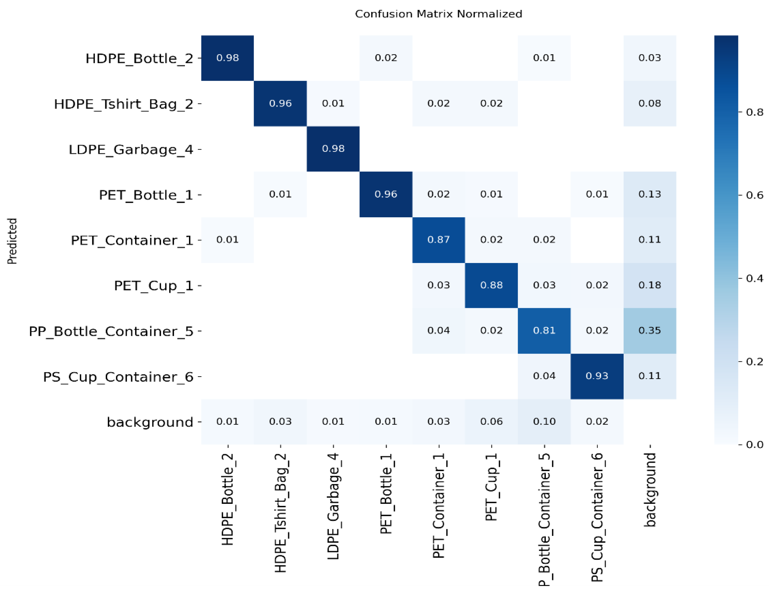
To examine class-wise behavior, a column-normalized confusion matrix was computed on the held-out test set (Figure 7), where columns represent ground truth classes and rows represent predicted labels. Diagonal entries indicate class-wise recall. The highest recall values were observed for HDPE_Bottle and LDPE_Garbage (0.98 each), followed by HDPE_Tshirt_Bag and PET_Bottle (0.96 each). Lower recall was observed for PET_Container (0.87), PET_Cup (0.88), and especially PP_Bottle_Container (0.81), while PS_Cup_Container remained comparatively stable (0.93). Most errors were associated with object–background ambiguity rather than strong cross-class confusion. In particular, PP_Bottle_Container showed the largest missed-detection and spurious-detection rates involving background. Despite these localized errors, the model maintained strong overall segmentation quality (mask mAP@50:95 $\approx 0.934$), supporting reliable aggregate-level downstream estimation.

4.3.3. Per-Class Precision–Recall Dynamics

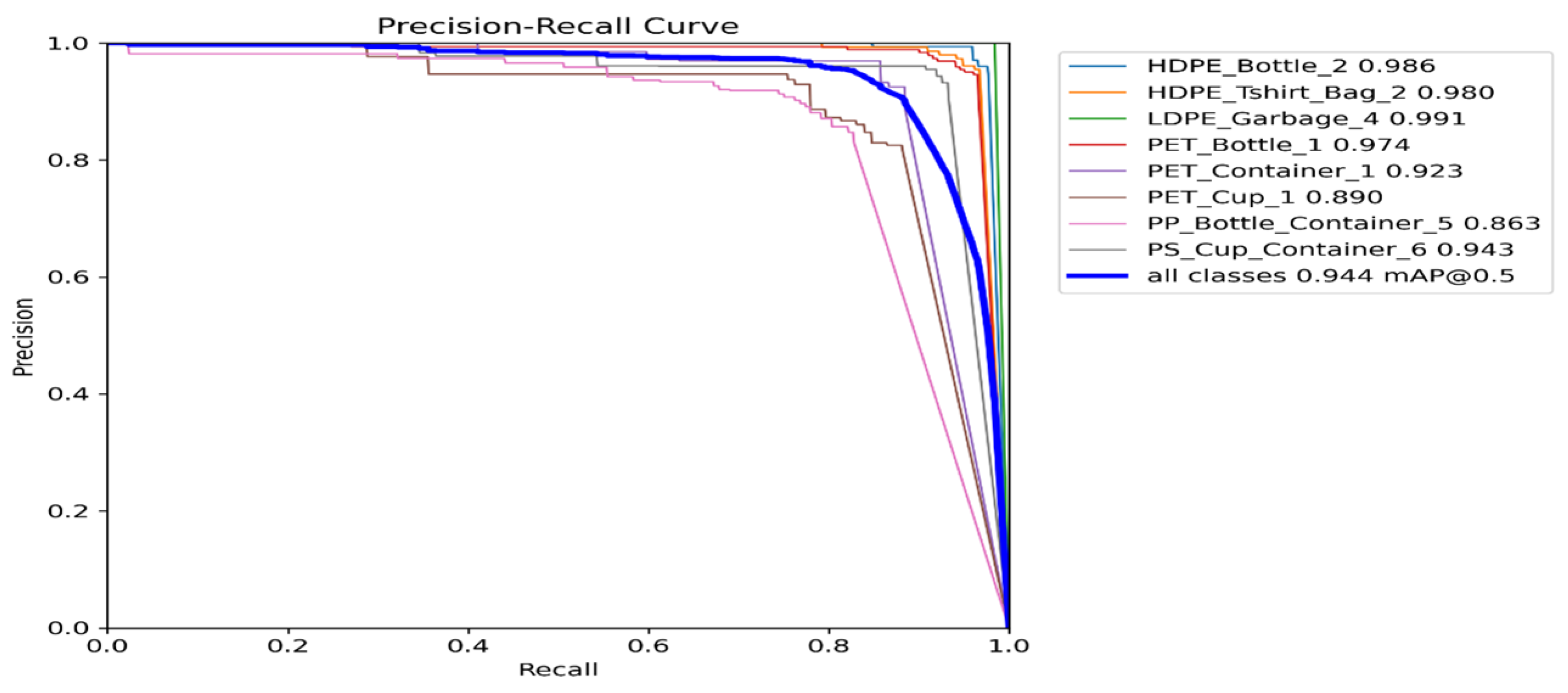
The class-wise precision–recall curves in Figure 8 show clear variation across polymer categories. The polyethylene classes, especially LDPE_Garbage and both HDPE categories, maintained the strongest curves, indicating high precision and stable recall. PET showed more mixed behavior: PET_Bottle remained strong, whereas PET_Cup and PET_Container degraded earlier, consistent with the effects of transparency and specular reflections. PS_Cup_Container maintained high precision with some recall loss, suggesting relatively conservative predictions. PP_Bottle_Container showed the weakest overall curve, likely due to broader within-class variability. Overall, performance degradation was driven mainly by recall loss in visually ambiguous plastics, while precision remained relatively high across classes. Although the dataset shows moderate variation in class frequencies, class-level performance differences are not explained by sample count alone. Deformation, occlusion, clutter, and inter-class visual similarity also affect segmentation difficulty. Weighted mAP and per-class threshold optimization were not included in the present uniform COCO-style evaluation and remain directions for future work. These class-wise results should also be interpreted in light of the evaluation protocol used in this study. Specifically, all model development decisions were made using the training and validation splits only, while the held-out test set remained locked until the final evaluation. The final generalization results therefore reflect performance on unseen test images that were not used for architecture screening, hyperparameter refinement, training strategy ablation, seed analysis, or NMS selection. In addition, the final model was not selected from a single favorable run, but was supported by the independent seed-robustness analysis reported in Stage 3B. At the same time, because multiple model selection stages were conducted using the same validation split, a residual risk of validation over-tuning cannot be fully excluded. Taken together, the locked test-set protocol and multi-seed robustness analysis reduce the likelihood that the reported test performance is driven by test-informed model selection or a single favorable initialization, although they do not eliminate all possible sources of residual dataset bias or validation-specific tuning effects.

4.4. State-of-the-Art Comparison

To contextualize the performance of the optimized YOLOv11s-seg model, we conducted a two-level evaluation: first, a controlled baseline comparison against alternative architectures trained on identical data, and second, a literature-based comparison with recent waste-segmentation studies. This isolates the contribution of architectural choice from dataset effects and clarifies the position of the proposed approach within the current research landscape.

4.4.1. Direct Baseline Comparison

The optimized YOLOv11s-seg model [37] was compared with YOLOv8s-seg [38], Mask R-CNN with a ResNet-50-FPN backbone [14,39,40], and the more recent transformer-based RF-DETR-Seg (Small) [41,42] using the same fixed train/validation/test split and the same held-out test set (Table 9). All models were evaluated under the COCO segmentation protocol, and framework-appropriate training settings were used to maintain a practically fair and reproducible comparison.

Comparison with YOLOv8s-Seg

YOLOv11s-seg achieved higher mask mAP@50:95 than YOLOv8s-seg (0.9337 vs. 0.9203; $\mathrm{\Delta }=+0.0134$), corresponding to an approximately 16.8% relative reduction in segmentation error. It also improved precision (0.9411 vs. 0.9049) and F1-score (0.9169 vs. 0.9010), while using fewer parameters (10.11M vs. 11.82M). Recall was slightly lower (0.8939 vs. 0.8971).

Comparison with Mask R-CNN

Compared with Mask R-CNN, YOLOv11s-seg improved mask mAP@50:95 from 0.8754 to 0.9337 ($\mathrm{\Delta }=+0.0583$), corresponding to an approximately 46.8% relative reduction in segmentation error. It also increased precision (0.9411 vs. 0.8315) and F1-score (0.9169 vs. 0.8794), while using far fewer parameters (10.11M vs. 43.96M), although Mask R-CNN achieved higher recall (0.9331 vs. 0.8939).

Comparison with RF-DETR-Seg (Small)

RF-DETR-Seg (Small) provided a stronger modern baseline and achieved a competitive mask mAP@50:95 of 0.9222. Nevertheless, YOLOv11s-seg still achieved the best performance on the primary segmentation metric used in this study, improving mask mAP@50:95 by +0.0115 (0.9337 vs. 0.9222), which corresponds to an approximately 14.8% relative reduction in segmentation error. YOLOv11s-seg also achieved higher precision (0.9411 vs. 0.9309) while using substantially fewer parameters (10.11M vs. 33.7M). However, RF-DETR-Seg (Small) obtained slightly higher recall (0.9232 vs. 0.8939) and F1-score (0.9268 vs. 0.9169). These results indicate that the proposed YOLOv11s-seg model remained the strongest method in terms of mask mAP@50:95, while RF-DETR-Seg (Small) served as a strong competitive transformer-based baseline.

4.4.2. Literature Comparison

To position the proposed model within the broader literature, we reviewed recent deep learning-based waste analysis methods that used instance segmentation, object detection, or related quantification pipelines.

Table 10. Comparative analysis of state-of-the-art waste segmentation and related quantification methods.

Reference	Year	Architecture	Dataset Size	Inst.	Mass	Env.	Uncert.
Iliushina et al. [5]	2025	YOLOv8-seg	4000 images	✓	×	×	×
Son & Ahn [10]	2025	YOLOv8-seg/Mask R-CNN	1800 images	✓	×	×	×
Sirimewan [59]	2025	Vision Transformer	5413 objects	✓	×	×	×
Alsuwaylimi [60]	2024	YOLOv8-Seg (RepBlock)	TrashCan (mixed)	✓	×	×	×
Díaz-Romero [12]	2022	DenseNet + BPNN	∼300 objects	×	✓	×	RMSE
This Work	2026	Optimized YOLOv11s-seg	4561 objects	✓	✓	✓	✓

Inst. = Instance Segmentation; Mass = Mass Estimation; Env. = Environmental Analysis; Uncert. = Uncertainty Quantification; ✓ = present; × = not reported.

summarizes the main characteristics of these studies alongside the proposed approach.

Segmentation Performance and Operational Gaps

Recent waste-focused studies [5,10,59,60] commonly report performance using mAP@50 (≈0.63–0.92), which is not directly comparable to COCO-style mask mAP@50:95. Under the present evaluation protocol, the proposed model achieved mask mAP@50:95 = 0.9337—a stricter metric than mAP@50—indicating strong segmentation robustness across IoU thresholds. Although its latency (150.86 ms/image, corresponding to approximately 6.6 fps under single-image inference on an NVIDIA A100 GPU) is higher than that of some ultra-fast specialized setups such as [60], this throughput provides a practical accuracy–efficiency balance while preserving the mask fidelity required for reliable downstream mass and environmental estimation.

The Mass Estimation Bottleneck

Díaz-Romero et al. [12] represent the main prior example linking vision to mass estimation ($R^2=0.82$ for metals), but three constraints limit its transferability to plastic waste: (1) rigid metal models do not reflect deformable polymer geometry; (2) reliance on RGB-D sensing increases hardware cost and maintenance complexity; and (3) single-object processing is incompatible with cluttered, continuous waste streams. In contrast, the present physics-informed approach operates on standard RGB imagery and estimates mass through material-specific density and thickness priors rather than purely data-driven regression.

Synthesis: From Detection to Valorization

Current literature can be grouped into three maturity tiers:

• Tier 1: Detection Centric [5,10,59,60].These studies optimize visual segmentation or detection accuracy but do not extend to physical quantification or downstream facility analysis.
• Tier 2: Partial Quantification [12]. These works demonstrate mass-estimation feasibility, but remain limited to single objects and rigid materials such as scrap metals.
• Tier 3: Integrated Valorization (This Work). The proposed framework links instance segmentation, mask-based mass estimation, and environmental impact assessment, while incorporating study-level scenario-based uncertainty ranges (±7–12%, depending on the derived output) and multi-seed robustness ($\mathrm{CV}=0.34\%$ across validation mAP@50:95). This extends waste-scene perception toward actionable facility-level analysis.

4.5. Qualitative Visual Evidence

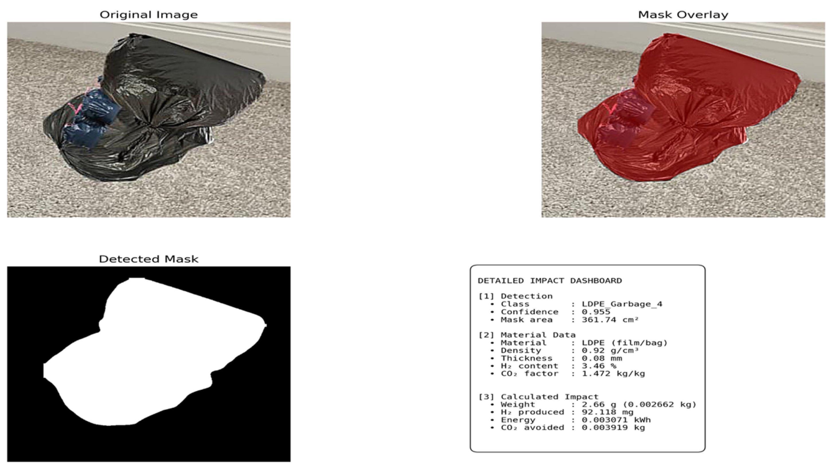
• Opaque Film (LDPE, Figure 9): This example illustrates a clear success case for opaque materials. The predicted mask is compact and contiguous, tightly matching the object silhouette with high confidence (∼0.955) and minimal background leakage. This supports reliable downstream mask-to-mass conversion.
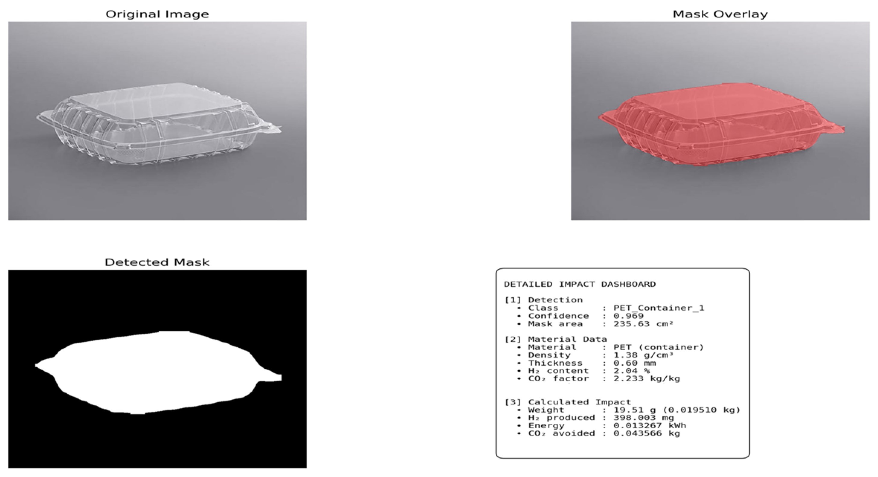
• Transparent Rigid Packaging (PET, Figure 10): This example highlights the optical complexity of PET. Although the object is correctly segmented with very high confidence (∼0.969), transparent edges and specular contours remain the main source of boundary ambiguity. This supports the conclusion that PET errors are driven primarily by object–background separability, often producing conservative masks rather than strong class confusion.

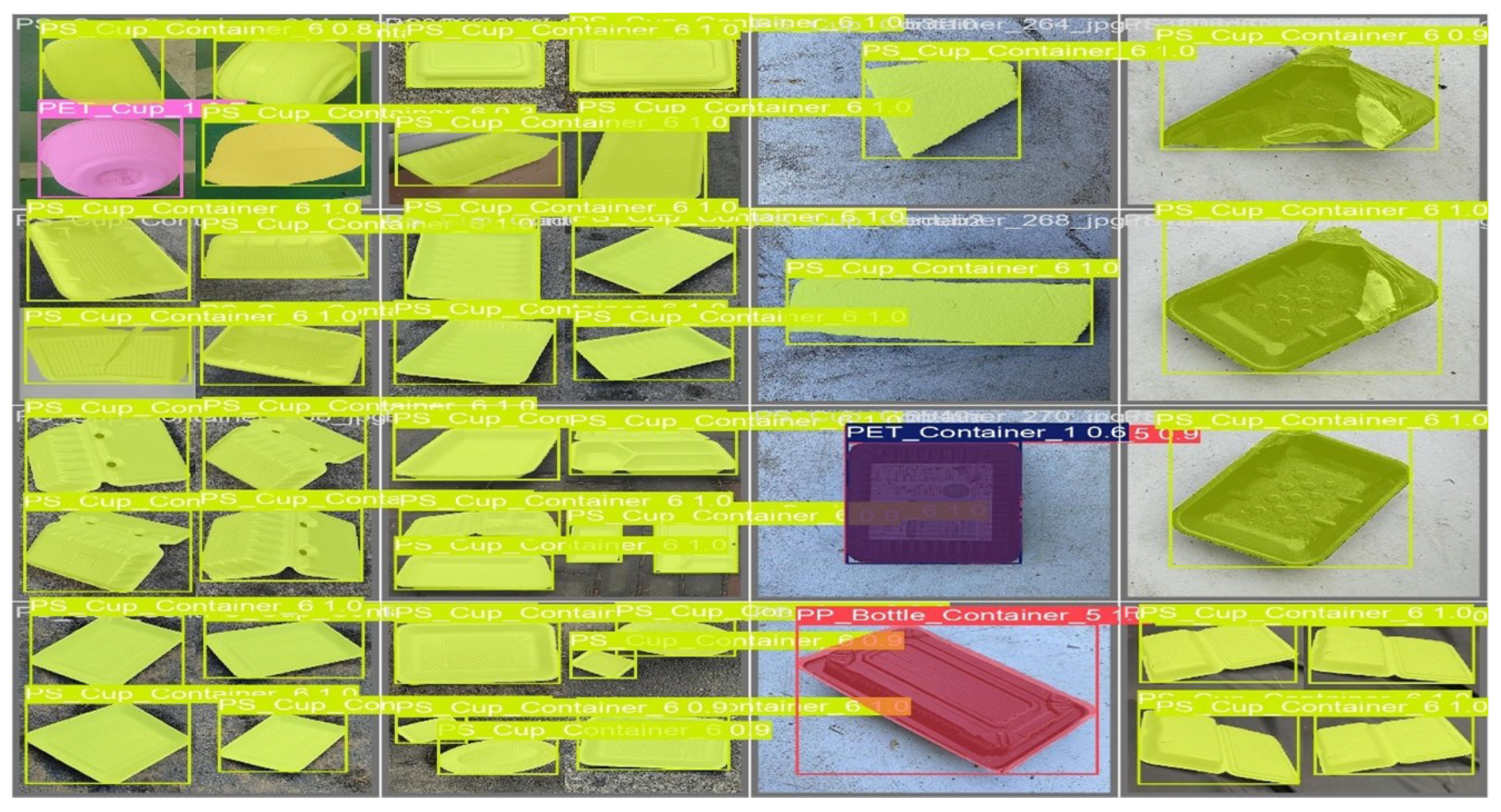
To complement the quantitative evaluation, Figure 11 provides a qualitative example for the PP_Bottle_Container class, which recorded the lowest recall among the evaluated categories. The figure illustrates the predicted segmentation behavior in a challenging mixed-waste scene and highlights how object shape, orientation, and scene composition can affect mask delineation quality. In particular, the dominant presence of PS_Cup_Container instances in close spatial proximity increases scene complexity and therefore offers qualitative context for the relatively lower recall observed for this class in the quantitative evaluation.

4.6. Environmental Impact and Valorization Analysis

To translate segmentation outputs into facility-level quantitative indicators, predicted instance masks were coupled with the physics-informed density/thickness model described in Phase III. Because no gravimetric ground truth mass measurements were available for the held-out test images, the resulting quantities are reported as indicative, assumption-based stream-level estimates rather than directly validated physical measurements. Environmental value is reported under an operational counting scenario based on $N=1253$ model detections (post-filtering) on the held-out test split, which is intentionally distinct from the ground truth count used for performance evaluation.

Material-Level Mass Quantification

The system produced an indicative total plastic mass estimate of 15.48 kg (±1.08 kg) from 1253 post-filtered detections across 868 test images. As shown in

Table 11. Prediction-based mass estimates and pathway-specific valorization indicators by material type for the test-stream scenario ($N=1253$).

Material	Count	Est. Mass (kg)	Hydrogen Recovery Pathway		Recycling Substitution Pathway
			H2 Potential (kg)	H2 Energy (kWh)	CO2e Avoided (kg)
PET	449	4.50	0.092	3.06	10.05
PS	167	5.43	0.129	4.31	15.83
PP	176	3.44	0.112	3.74	5.33
HDPE	335	1.92	0.069	2.30	3.09
LDPE	126	0.19	0.006	0.22	0.27
TOTAL	1253	15.48 ± 1.08	0.41 ± 0.04	13.63 ± 1.09	34.57 ± 4.15

, PS contributed the largest mass share (5.43 kg, ∼35%) and nearly 46% of the total potential CO₂ avoidance (15.83 kg), even though PET was the most frequent class (∼36% of detections). This indicates that environmental value is not proportional to object count and highlights the importance of accurate class-level mass estimation for impact-oriented analysis.

The values reported in Table 11 are prediction-based estimates derived from the proposed segmentation-to-mass pipeline and class-specific conversion assumptions. Because no direct measured ground truth mass was available for the analyzed stream, these results should be interpreted as indicative stream-level estimates rather than experimentally validated physical measurements.

4.7. Limitations and Future Scope

The proposed framework has important limitations. First, mass estimation is based on a sheet-equivalent approximation from 2D mask area and a fixed nominal scale factor ($\alpha =0.05$ cm/pixel) applied uniformly across all images. Because the dataset aggregates images from heterogeneous sources with varying acquisition distances, the reported uncertainty ranges should be interpreted as scenario-based bounds rather than formal metrological confidence intervals. Accordingly, absolute mass values carry systematic uncertainty beyond the reported bounds and should be treated as order-of-magnitude stream-level estimates rather than direct physical measurements. This approximation may additionally be less reliable for heavily deformed or crushed items. Moreover, no direct gravimetric ground truth comparison was available for the estimated masses in the present dataset, so the absolute accuracy of the mask-to-mass module could not be experimentally established within the current study. In addition, the benchmark was curated to preserve the empirical class frequencies observed after dataset assembly, without artificial resampling or class-balancing interventions, so that the evaluation reflects naturally occurring category prevalence within the assembled multi-source setting. However, because the benchmark combines multiple external sources, residual source-specific dataset bias cannot be fully excluded without a dedicated source-stratified analysis. Moreover, because the staged model selection procedure was performed repeatedly on the same validation split, some residual risk of validation-specific over-tuning remains, even though the held-out test set was kept fully locked until the final evaluation. Second, the use of nominal material properties does not capture real-world contamination, such as residual contents or adhering debris. Third, the current evaluation is based on static imagery and does not fully reflect live conveyor-belt conditions, including motion blur, occlusion, and variable illumination. A systematic comparison of augmentation strategies, including a no-augmentation baseline and alternative transformation sets, is left for future investigation, as the present study prioritized controlled ablation of architecture, training configuration, and validation-driven model selection over augmentation-policy search. Future work will focus on integrating depth sensing for improved volumetric estimation and per-image geometric calibration, validating the system under real industrial conditions, including direct comparison against measured object-level and stream-level mass values under controlled acquisition settings, and extending the framework to broader waste categories, including glass, metal, and composite packaging materials, which introduce additional appearance and material heterogeneity beyond the present plastic-focused setting.

5. Conclusions

This study presents a multi-stage YOLOv11-based framework for robust instance segmentation and material quantification of mixed plastic waste. The proposed pipeline integrates validation-driven model optimization, a controlled evaluation protocol, and post-segmentation mass estimation within a unified system designed for reliable performance under heterogeneous waste-scene conditions.

Experimental results on the held-out test set demonstrate the effectiveness of the optimized YOLOv11s-seg model, which achieved a mask mAP@50:95 of 0.9337, a precision of 0.9411, and an F1-score of 0.9169. These results support reliable mask-based estimation beyond conventional recognition-only reporting. Applied to the held-out test stream ($N=1253$ detected objects), the framework estimated an indicative total plastic mass of 15.48 ± 1.08 kg, corresponding to a theoretical potential of 0.41 ± 0.04 kg H₂ and 34.57 ± 4.15 kg CO₂e avoidance under alternative valorization pathways.

A key insight of this work is that downstream value is not directly proportional to detection frequency. While polystyrene (PS) was not the most frequent category, it accounted for approximately 46% of the total CO₂e avoidance (15.83 kg), highlighting the importance of composition-aware quantification in recovery-oriented decision support.

Overall, the proposed framework extends waste-scene understanding beyond vision-level assessment toward physically grounded, data-driven support for material-aware recovery systems. Future research will focus on RGB-D integration for enhanced volumetric estimation, temporal modeling to handle dynamic conveyor-belt conditions, and the extension of the framework to include a broader range of multi-material waste streams.

References

1. Geyer, R.; Jambeck, J.R.; Law, K.L. Production, use, and fate of all plastics ever made. Sci. Adv. 2017, 3, e1700782. [Google Scholar] [CrossRef] [PubMed]
2. OECD. Global Plastics Outlook: Policy Scenarios to 2060; OECD Publishing: Paris, France, 2022; Available online: https://www.oecd.org/en/publications/2022/06/global-plastics-outlook_f065ef59.html (accessed on 7 April 2026).
3. United Nations Environment Programme (UNEP). Turning Off the Tap: How the World Can End Plastic Pollution and Create a Circular Economy; UNEP: Nairobi, Kenya, 2023; Available online: https://www.unep.org/resources/turning-off-tap-end-plastic-pollution-create-circular-economy (accessed on 7 April 2026).
4. Niu, F.; Wu, Z.; Chen, D.; Huang, Y.; Ordomsky, V.V.; Khodakov, A.Y.; Van Geem, K.M. State-of-the-art and perspectives of hydrogen generation from waste plastics. Chem. Soc. Rev. 2025, 54, 4948–4972. [Google Scholar] [CrossRef] [PubMed]
5. Iliushina, A.; Mazanov, G.; Nesteruk, S.; Pimenov, A.; Stepanov, A.; Mikhaylova, N.; Baldycheva, A.; Somov, A. Data-centric approach for instance segmentation in optical waste sorting. Waste Manag. 2025, 191, 70–80. [Google Scholar] [CrossRef] [PubMed]
6. Jaikumar, P.; Vandaele, R.; Ojha, V. Transfer Learning for Instance Segmentation of Waste Bottles Using Mask R-CNN Algorithm. In Intelligent Systems Design and Applications (ISDA 2020); Springer: Cham, Switzerland, 2021; pp. 140–149. [Google Scholar] [CrossRef]
7. Sayem, F.R.; Islam, M.S.B.; Naznine, M.; Nashbat, M.; Hasan-Zia, M.; Kunju, A.K.A.; Khandakar, A.; Ashraf, A.; Majid, M.; Kashem, S.; et al. Enhancing waste sorting and recycling efficiency: Robust deep learning-based approach for classification and detection. Neural Comput. Appl. 2025, 37, 4567–4583. [Google Scholar] [CrossRef]
8. Mao, W.-L.; Chen, W.-C.; Wang, C.-T.; Lin, Y.-H. Recycling waste classification using optimized convolutional neural network. Resour. Conserv. Recycl. 2021, 164, 105132. [Google Scholar] [CrossRef]
9. Gawlikowski, J.; Tassi, C.R.N.; Ali, M.; Lee, J.; Humt, M.; Feng, J.; Kruspe, A.; Triebel, R.; Jung, P.; Roscher, R.; et al. A survey of uncertainty in deep neural networks. Artif. Intell. Rev. 2023, 56, 1513–1589. [Google Scholar] [CrossRef]
10. Son, J.; Ahn, Y. AI-based plastic waste sorting method utilizing object detection models for enhanced classification. Waste Manag. 2025, 193, 273–282. [Google Scholar] [CrossRef] [PubMed]
11. Standley, T.; Sener, O.; Chen, D.; Savarese, S. Image2Mass: Estimating the Mass of an Object from Its Image. In Proceedings of the 1st Annual Conference on Robot Learning (CoRL), Mountain View, CA, USA, 13–15 November 2017; PMLR: New York, NY, USA, 2017; Volume 78, pp. 324–333. [Google Scholar]
12. Díaz-Romero, D.; Van den Eynde, S.; Sterkens, W.; Engelen, B.; Zaplana, I.; Dewulf, W.; Goedemé, T.; Peeters, J. Simultaneous mass estimation and class classification of scrap metals using deep learning. Resour. Conserv. Recycl. 2022, 181, 106272. [Google Scholar] [CrossRef]
13. Liang, S.; Gu, Y. A deep convolutional neural network to simultaneously localize and recognize waste types in images. Waste Manag. 2021, 126, 247–257. [Google Scholar] [CrossRef] [PubMed]
14. He, K.; Gkioxari, G.; Dollár, P.; Girshick, R. Mask R-CNN. IEEE Trans. Pattern Anal. Mach. Intell. 2020, 42, 386–397. [Google Scholar] [CrossRef] [PubMed]
15. Kataoka, T.; Yoshida, T.; Yamamoto, N. Instance segmentation models for detecting floating macroplastic debris from river surface images. Front. Earth Sci. 2024, 12, 1427132. [Google Scholar] [CrossRef]
16. Wang, M.; Deng, W. Deep visual domain adaptation: A survey. Neurocomputing 2018, 312, 135–153. [Google Scholar] [CrossRef]
17. Smith, L.N. A disciplined approach to neural network hyper-parameters: Part 1—Learning rate, batch size, momentum, and weight decay. arXiv 2018, arXiv:1803.09820. [Google Scholar] [CrossRef]
18. Li, L.; Jamieson, K.; DeSalvo, G.; Rostamizadeh, A.; Talwalkar, A. Hyperband: A Novel Bandit-Based Approach to Hyperparameter Optimization. J. Mach. Learn. Res. 2018, 18, 1–52. [Google Scholar]
19. Yosinski, J.; Clune, J.; Bengio, Y.; Lipson, H. How transferable are features in deep neural networks? In Advances in Neural Information Processing Systems 27 (NeurIPS 2014), Montréal, QC, Canada, 8–13 December 2014; Curran Associates, Inc.: Red Hook, NY, USA, 2014; pp. 3320–3328. Available online: https://proceedings.neurips.cc/paper_files/paper/2014/hash/532a2f85b6977104bc93f8580abbb330-Abstract.html (accessed on 7 April 2026).
20. Henderson, P.; Islam, R.; Bachman, P.; Pineau, J.; Precup, D.; Meger, D. Deep reinforcement learning that matters. In Proceedings of the AAAI Conference on Artificial Intelligence, New Orleans, LA, USA, 2–7 February 2018; AAAI Press: Washington, DC, USA, 2018; Volume 32, pp. 3207–3214. [Google Scholar] [CrossRef]
21. Wang, H.; Liu, H.; Lu, X.; Zhang, Z. Image2Mass++: Hybrid Condition-Guided Mass Estimation from a Single Image. Measurement 2026, 260, 119876. [Google Scholar] [CrossRef]
22. Guo, C.; Pleiss, G.; Sun, Y.; Weinberger, K.Q. On Calibration of Modern Neural Networks. In Proceedings of the 34th International Conference on Machine Learning (ICML), Sydney, NSW, Australia, 6–11 August 2017; PMLR: New York, NY, USA, 2017; Volume 70, pp. 1321–1330. Available online: https://proceedings.mlr.press/v70/guo17a.html (accessed on 7 April 2026).
23. Single, S.; Iranmanesh, S.; Raad, R. RealWaste [Dataset]. UCI Machine Learning Repository. 2023. Available online: https://archive.ics.uci.edu/dataset/908/realwaste (accessed on 7 April 2026).
24. Snowman1908. Plastic Recyclable Detection Dataset; Roboflow Universe: Des Moines, IA, USA, 2025; Available online: https://universe.roboflow.com/snowman1908/plastic-recyclable-detection (accessed on 7 April 2026).
25. King, A. Recyclable and Household Waste Classification; Kaggle: San Francisco, CA, USA, 2019; Available online: https://www.kaggle.com/datasets/alistairking/recyclable-and-household-waste-classification (accessed on 7 April 2026).
26. Serezhkin, A. Drinking Waste Classification; Kaggle: San Francisco, CA, USA, 2020; Available online: https://www.kaggle.com/datasets/arkadiyhacks/drinking-waste-classification (accessed on 7 April 2026).
27. Roboflow. Plastic Waste Detection; Dataset v1; Roboflow Universe: San Francisco, CA, USA, 2024; Available online: https://universe.roboflow.com/ta-lulus/plastic-waste-detection-gtkyw/dataset/1 (accessed on 7 April 2026).
28. Torralba, A.; Efros, A.A. Unbiased look at dataset bias. In Proceedings of the IEEE Conference on Computer Vision and Pattern Recognition (CVPR), Colorado Springs, CO, USA, 20–25 June 2011; IEEE: New York, NY, USA, 2011; pp. 1521–1528. [Google Scholar] [CrossRef]
29. ASTM D7611/D7611M-20; Standard Practice for Coding Plastic Manufactured Articles for Resin Identification. ASTM International: West Conshohocken, PA, USA, 2020.
30. Padalkar, A.S.; Pathak, P.; Stynes, P. An Object Detection and Scaling Model for Plastic Waste Sorting. In Proceedings of the 1st International Conference on AI for People: Towards Sustainable AI (CAIP 2021), Bologna, Italy, 20–24 November 2021; EAI: Seoul, Republic of Korea, 2021. [Google Scholar] [CrossRef]
31. ITU-T. Digital Compression and Coding of Continuous-Tone Still Images (JPEG); Recommendation T.81; ITU-T: Geneva, Switzerland, 1992. [Google Scholar]
32. Roboflow Inc. Roboflow: Computer Vision Tools for Developers; Roboflow Inc.: Des Moines, IA, USA, 2020; Available online: https://roboflow.com (accessed on 7 April 2026).
33. Lin, T.-Y.; Maire, M.; Belongie, S.; Bourdev, L.; Girshick, R.; Hays, J.; Perona, P.; Ramanan, D.; Zitnick, C.L.; Dollár, P. Microsoft COCO: Common objects in context. In Proceedings of the European Conference on Computer Vision (ECCV), Zurich, Switzerland, 6–12 September 2014; Springer: Cham, Switzerland, 2014; pp. 740–755. [Google Scholar] [CrossRef]
34. Roboflow. Preprocess Images. Roboflow Docs. Available online: https://docs.roboflow.com/datasets/dataset-versions/image-preprocessing (accessed on 15 April 2026).
35. Goodfellow, I.; Bengio, Y.; Courville, A. Deep Learning; MIT Press: Cambridge, MA, USA, 2016. [Google Scholar]
36. Shorten, C.; Khoshgoftaar, T.M. A survey on image data augmentation for deep learning. J. Big Data 2019, 6, 60. [Google Scholar] [CrossRef]
37. Ultralytics. YOLO11. Ultralytics YOLO Docs; Ultralytics Inc.: San Diego, CA, USA, 2024; Available online: https://docs.ultralytics.com/models/yolo11/ (accessed on 15 April 2026).
38. Ultralytics. YOLOv8 Instance Segmentation. In Ultralytics YOLO Docs; Ultralytics Inc.: San Diego, CA, USA, 2023; Available online: https://docs.ultralytics.com/tasks/segment/ (accessed on 15 April 2026).
39. He, K.; Zhang, X.; Ren, S.; Sun, J. Deep residual learning for image recognition. In Proceedings of the IEEE Conference on Computer Vision and Pattern Recognition (CVPR), Las Vegas, NV, USA, 27–30 June 2016; IEEE: New York, NY, USA, 2016; pp. 770–778. Available online: https://ieeexplore.ieee.org/document/7780459 (accessed on 15 April 2026).
40. Lin, T.-Y.; Dollár, P.; Girshick, R.; He, K.; Hariharan, B.; Belongie, S. Feature pyramid networks for object detection. In Proceedings of the IEEE Conference on Computer Vision and Pattern Recognition (CVPR), Honolulu, HI, USA, 21–26 July 2017; IEEE: New York, NY, USA, 2017; pp. 2117–2125. [Google Scholar] [CrossRef]
41. Robinson, I.; Robicheaux, P.; Popov, M.; Ramanan, D.; Peri, N. RF-DETR: Neural architecture search for real-time detection transformers. arXiv 2025, arXiv:2511.09554. [Google Scholar] [CrossRef]
42. Roboflow. RF-DETR Segmentation. Available online: https://roboflow.com/model/rf-detr-segmentation (accessed on 15 April 2026).
43. ISO 17855-2; Plastics—Polyethylene (PE) Moulding and Extrusion Materials—Part 2: Preparation of Test Specimens and Determination of Properties. ISO: Geneva, Switzerland, 2024.
44. ISO 17855-1; Plastics—Polyethylene (PE) Moulding and Extrusion Materials—Part 1: Designation System and Basis for Specifications. ISO: Geneva, Switzerland, 2014.
45. ISO 12418-1; Plastics—Post-Consumer Poly(ethylene terephthalate) (PET) Bottle Recyclates—Part 1: Designation System and Basis for Specifications. ISO: Geneva, Switzerland, 2012.
46. ISO 19069-1; Plastics—Polypropylene (PP) Moulding and Extrusion Materials—Part 1: Designation System and Basis for Specifications. ISO: Geneva, Switzerland, 2015.
47. ISO 1622-1; Plastics—Polystyrene (PS) Moulding and Extrusion Materials—Part 1: Designation System and Basis for Specifications. ISO: Geneva, Switzerland, 2012.
48. ASTM D4976-21; Standard Specification for Polyethylene Plastics Molding and Extrusion Materials. ASTM International: West Conshohocken, PA, USA, 2021.
49. Brandrup, J.; Immergut, E.H.; Grulke, E.A. (Eds.) Polymer Handbook, 4th ed.; Wiley-Interscience: New York, NY, USA, 1999. [Google Scholar]
50. American Chemistry Council. Cradle-to-Gate Life Cycle Analysis of High-Density Polyethylene (HDPE) Resin; American Chemistry Council: Washington, DC, USA, 2020; Available online: https://www.americanchemistry.com/content/download/8059/file/Cradle-to-Gate-Life-Cycle-Analysis-of-High-Density-Polyethylene-HDPE-Resin.pdf (accessed on 7 April 2026).
51. American Chemistry Council. Cradle-to-Gate Life Cycle Analysis of Polypropylene (PP) Resin; American Chemistry Council: Washington, DC, USA, 2021; Available online: https://www.americanchemistry.com/content/download/8063/file/Cradle-to-Gate-Life-Cycle-Analysis-of-Polypropylene-PP-Resin.pdf (accessed on 7 April 2026).
52. American Chemistry Council. Cradle-to-Gate Life Cycle Analysis of General Purpose Polystyrene (GPPS) Resin; American Chemistry Council: Washington, DC, USA, 2022; Available online: https://www.americanchemistry.com/content/download/10598/file/Cradle-to-Gate-Life-Cycle-Analysis-of-General-Purpose-Polystyrene-Resin.pdf (accessed on 7 April 2026).
53. Franklin Associates; A Division of ERG. Cradle-to-Resin Life Cycle Analysis of Polyethylene Terephthalate Resin: Final Revised Report. 2020. Available online: https://napcor.com/wp-content/uploads/2020/05/Final-Revised-Virgin-PET-Resin-LCA.pdf (accessed on 21 April 2026).
54. American Chemistry Council. Cradle-to-Gate Life Cycle Analysis of Linear Low-Density Polyethylene (LLDPE) Resin; American Chemistry Council: Washington, DC, USA, 2020; Available online: https://www.americanchemistry.com/content/download/8061/file/cradle-to-gate-life-cycle-analysis-of-linear-low-density-polyethylene-lldpe-resin.pdf (accessed on 7 April 2026).
55. Aminu, I.; Nahil, M.A.; Williams, P.T. Pyrolysis-plasma/catalytic reforming of post-consumer waste plastics for hydrogen production. Catal. Today 2023, 420, 114084. [Google Scholar] [CrossRef]
56. ISO 14040; Environmental Management—Life Cycle Assessment—Principles and Framework. ISO: Geneva, Switzerland, 2006.
57. ISO 14044; Environmental Management—Life Cycle Assessment—Requirements and Guidelines. ISO: Geneva, Switzerland, 2006.
58. Uusitalo, T.; Toukoniitty, E. Environmental Impacts of Plastic Recycling: A Literature Review; VTT Research Report VTT-R-00604-24; VTT Technical Research Centre of Finland: Espoo, Finland, 2024. [Google Scholar]
59. Sirimewan, D.; Dayarathna, S.; Raman, S.; Bai, Y.; Arashpour, M. A benchmark dataset for class-wise segmentation of construction and demolition waste in cluttered environments. Sci. Data 2025, 12, 885. [Google Scholar] [CrossRef] [PubMed]
60. Alsuwaylimi, A.A. Enhanced YOLOv8-Seg instance segmentation for real-time submerged debris detection. IEEE Access 2024, 12, 117833–117849. [Google Scholar] [CrossRef]
Figure 1. Phase I pipeline of the proposed framework, illustrating dataset collection, annotation, splitting, preprocessing, and augmentation steps.
Computers 15 00271 g001
Figure 2. Representative visual examples of the eight operational plastic waste categories used in this study, defined by the combination of polymer type and physical form.
Computers 15 00271 g002
Figure 3. Representative example of the annotation workflow used in this study: (a) original image, (b) polygon-based instance annotation created in Roboflow, and (c) resulting mask visualization for instance segmentation training and evaluation.
Computers 15 00271 g003
Figure 4. Phase II: Four-stage sequential model development and selection protocol.
Computers 15 00271 g004
Figure 5. Phase III pipeline for final evaluation and environmental impact analysis.
Computers 15 00271 g005
Figure 6. Conceptual workflow linking instance segmentation to projected area, class-resolved mass estimation, and downstream hydrogen recovery, CO2e-avoidance, and primary-energy indicators. Mask mAP@50:95 is a segmentation-quality indicator, not a direct downstream input.
Computers 15 00271 g006
Figure 7. Column-normalized confusion matrix on the test set.
Computers 15 00271 g007
Figure 8. Mask precision–recall curves per class on the test set.
Computers 15 00271 g008
Figure 9. Opaque LDPE segmentation (Conf. 0.955) exhibiting precise boundary localization due to high contrast.
Computers 15 00271 g009
Figure 10. Transparent PET segmentation (Conf. 0.969) demonstrating robust detection against specular reflections and optical ambiguity.
Computers 15 00271 g010
Figure 11. Qualitative example for PP_Bottle_Container, showing segmentation behavior in a challenging mixed-waste scene and helping explain the lower recall observed for this class.
Computers 15 00271 g011