MindVoice: A Web-Based Multi-Dataset Speech Depression Screening System with Pipeline-Aware Grad-CAM Explainability

Abstract

Although speech-based depression assessment has received considerable attention, achieving reliable confidence and cross-corpus applicability with explanation of prediction still remains challenging. This study presents a reliability-aware framework for speech-only depression severity assessment and its deployment through MindVoice. The distress analysis interview corpus (DAIC), extended distress analysis interview corpus (E-DAIC) and multimodal open dataset for mental disorder analysis (MODMA) are integrated to form a heterogeneous multi-corpus cross-lingual dataset of three classes. The Audio-Textual Depression Corpus (EATD) is also evaluated for four classes. Domain-specific feature normalization is applied to reduce variations arising from differences among the datasets. CNN-derived speech representations are subsequently refined through Analysis of Variance (ANOVA) followed by artificial bee colony (ABC)-based feature optimization, and an MLP assigns samples to severity levels. To improve the trustworthiness of predicted probabilities, seven calibration approaches like Temperature, Platt (Sigmoid), Isotonic, Vector, Matrix, Dirichlet, and Beta calibration are compared using accuracy and Expected calibration error. Reliability is quantified using a fixed-weight combination of bin-based reliability (0.7) and entropy (0.3) while comparing with other reliability assessment methods. A pipeline-aware gradient-weighted class activation mapping approach is proposed that enables explanations by reconstructing sklearn components as Tensorflow components for gradient backpropagation across the hybrid pipeline. The framework obtains 76.5% accuracy on the combined corpus, while the DAIC, E-DAIC, and MODMA achieve an accuracy of 81.4%, 72% and 80% respectively, and the EATD achieves 78.5% accuracy for 4-class classification. The proposed framework provides effective classification for a heterogeneous dataset. Its deployment on the web as the MindVoice application inculcates reliability-aware and explainable prediction that provides a more trustworthy system than the conventional performance-only assessment.

1. Introduction

Depression, a mental health disorder, is devastating the generations. As per the WHO, depression, which is also called Major Depressive Disorder (MDD), is prevailing among 332 million people across the world [1]. It not only makes people suffer in constant sadness but also affects their thinking and behavior. It also influences characteristics of speech such as prosody, speaking rate, voice quality, and temporal/acoustic patterns. A depressed person becomes disabled to perform even daily tasks. Early detection and intervention is key to reducing the suffering which is still limited due to limitations of clinics for mental health and due to the taboo associated with it. In such a situation, the need for an accessible tool for depression detection becomes a necessity. Initially, a questionnaire-based mobile application was launched, but the user bias involved in it let researchers think about other tools such as speech.

With the advancement of feature extraction, classification mechanisms and machine learning and deep learning techniques, a broad area of research for depression detection using speech has opened up [2]. Speech is a non-invasive and relatively easy to collect mode that makes an app based on such frameworks deployable. However, speech-based depression detection frameworks are subjective to dataset and evaluation protocols. Different datasets differ in language, recording environment and interview style due to which a model that is achieving high performance may not perform the same on another dataset.

A combined multi-dataset database can be an attempt to allow the model to learn representations regardless of the source. However, this does not ensure that underlying distributions become equivalent [3]. A domain-adaptation strategy such as domain-specific feature normalization must be applied for normalizing the scale of every dataset, such as the DAIC, E-DAIC and MODMA, separately so that the features generated from different datasets become indistinguishable. There will still be differences that cannot be solved by simple domain adaptation.

If the discussion is about web-based deployment of the model, the trustworthiness of prediction becomes crucial which is still an unexplored domain. Confidence of prediction, reliability of confidence and explanation of prediction are those elements that increase the trust over prediction. Such elements are crucial when a major decision is to be based on the results. Post hoc calibration provides a mechanism for improving confidence by comparing predicted and actual probabilities. Different calibration techniques are evaluated on the basis of the expected calibration error (ECE), Brier score, and negative log-likelihood (NLL), and the best calibration technique is selected and used [4]. This also encourages the estimation of reliability of this confidence. Various reliability estimations such as bin-accuracy, entropy and the Adaptive Reliability Score (ARS) are evaluated for providing an additional layer of information. Based on the results, a fixed-weighed formulation of 0.7 bin/0.3 entropy is finally used. Lastly, the need of explanation of prediction for increasing the interpretability is entertained by proposing a novel version of Grad-CAM termed as Pipeline-Aware Grad-CAM. PA-Grad-CAM reconstructs the hybrid pipeline used by the deployed model and enables the gradient backpropagation. Finally, a web-based application “MindVoice” is deployed constituting all the above features for ensuring trustworthy prediction of depression severity level. MindVoice is based on a model that uses an enhanced trained CNN for feature extraction, two-stage feature selection using ANOVA and ABC optimization and MLP for severity classification.

Hence, the gaps addressed in this work are as follows:

• Evaluation through a heterogeneous dataset composed of different languages, different recording conditions, etc.
• Calibration/reliability: Classification accuracy is not an indicator of trustworthiness of a system.
• Explainability: The lack of quantitatively verified modules for explaining which part of speech influences the prediction.
• Deployment: The ack of frameworks that are available on the web.

The contribution of the paper is summarized as follows:

• Speech based depression-severity framework development and evaluation through a heterogeneous dataset.
• Domain handling through domain-specific feature normalization.
• Calibration for confidence estimation.
• Proposing the Pipeline-Aware Grad-CAM explanation module.
• Integration of all the above in a web-based app, “MindVoice”.

The overall organization of the study is as follows. Section 2 covers the related work section that discusses available speech-based and multimodal depression detection, available work on calibration and explainability, frameworks including multiple datasets and prior works done regarding application development for depression detection. Section 3 explains the proposed framework at the model training level. This includes feature extraction, feature selection and classification. Section 4 explains the inference of the web-based screening system including calibration and PA-Grad-CAM-based interpretability. Finally, the Result and Discussion is covered in Section 5 followed by the Conclusion for discussing limitations and future work.

2. Related Work

2.1. Speech-Based Depression Detection

The first study of the relationship between speech and depression cues began in the year 1984 [5]. Considering speech as a non-invasive tool, this research area expanded exponentially. The evolution of technology started from handcrafted acoustic descriptors such as MFCCs, pitch, jitter, shimmer, formants and prosodic statistics to the application of pre-trained large Wav2Vec features for expanding the availability of larger feature resources [6,7,8]. The classification techniques evolved from machine learning classifiers such as SVM, Random Forest, etc., to deep learning classifiers such as CNN, RNN, Transformer and attention-based architectures [8,9,10,11]. Each stage provided better and automated extraction of features instead of slow handcrafted ones along with stronger classification capability. The most recent work in the field is the use of TFCA-ResNet18 with temporal–frequency–channel attention and POCAII optimization [12]. This work achieved an accuracy of 93%. However, the evaluation was limited to binary classification and two datasets only.

2.2. Multimodal Depression Detection

Other than speech, depression detection models based on other modalities have also evolved. These modalities consider modes such as video, images, text and speech. In this series of work, Depressformer works on image sequence-based depression estimation with the help of Video Swin Transformer fine-grained local-feature extraction and channel-attention [13]. DEP-Former uses audio and facial expression for depression recognition by applying a modality adapter, attention-index sharing, cross-attention and multimodal feature fusion [14]. A novel dual-modal audio–text fusion network called IntervoxNet was proposed. It uses a combination Mel-Spectrogram Transformer for audio and a BERT-CNN for text and for audio–text a temporal fusion mechanism is applied [15]. DEPART provides detection of depression as well as Parkinson’s disease along with interpretability. It uses body region extraction, CLIP-based visual encoding, Transformer-based temporal modeling, prototype-aware classification and a gradient-based attention map for introducing interpretability to the system [16]. IMDD-Net uses all modalities. For video, it uses TimeSformer; for audio, MFCC and eGeMAPS are used; and for text, BERT is used followed by multimodal fusion [17]. Despite the availability of the multimodal system, this paper persists in using only speech for detecting depression. The motivation behind this approach is to investigate the applicability of a reliability-aware and explainable speech-based multi-dataset depression severity assessment framework with low-burden computation and processing. As the multimodal systems provide good accuracy but also the need for computation requirements, synchronized data acquisition, preprocessing and privacy considerations also increase.

Table 1. Summary of prior depression detection works in all modalities with respective advantages and limitations.

Year	Study	Modality	Task	Method	Advantage	Limitation
2018	Jiang et al. [6]	Audio	Depression detection	Ensemble logistic regression using multiple speech features	Combines various speech attributes with an interpretable ML model	Binary classification only, dependent on handcrafted features
2020	Kumar et al. [10]	Questionnaire responses	Depression severity classification	Eight ML algorithms and hybrid models	Multiple severity levels	Prone to user bias
2024	Huang et al. [8]	Audio	Depression severity classification	wav2vec 2.0 and fine-tuning network	Extract features directly from raw speech	Evaluated on DAIC-WOZ only; cross-dataset validation insufficient
2024	Depressformer [13]	Video	Depression severity classification	Video Swin Transformer, fine-grained local features, channel-attention fusion	Captures fine-grained features of video	Greater computational burden than speech-only systems
2024	IntervoxNet [15]	Audio + text	Depression detection	Mel-Spectrogram Transformer for audio; BERT/CNN for text and attention fusion	Combines acoustic and linguistic information	Binary classification only, requires two synchronized modalities, single dataset evaluation
2025	DEP-Former [14]	Audio + facial expressions	Depression detection	Modality adapter, shared attention index, multimodal cross-attention	Uses facial and acoustic information	Binary classification only, requires two synchronized modalities
2025	IMDD-Net [17]	Audio + video + text	Depression severity estimation	TimeSformer for video, MFCC and eGeMAPS for audio and BERT for text	Integrates local and global information across three modalities	High computational complexity due to three modalities, single dataset evaluation
2026	Rezaee [12]	Audio	Depression detection	Optimized temporal–frequency–channel attention, interpretable acoustic–prosodic mapping	Combines temporal–frequency–channel attention and interpretable acoustic–prosodic mapping	Binary classification only
2026	DEPART [16]	Video	Depression detection	CLIP-based visual representation, temporal Transformer, prototype-aware modeling	Integrate interpretability into video-based depression detection	High computational load, binary classification only

summarizes the advantages and limitations of the existing work using all modalities.

2.3. Multi-Dataset Depression Detection

Various works in multi-dataset depression have been executed. The DAIC, E-DAIC, CMDC, EATD, MODMA, Android speech data, etc., were frequently used in various works for analyzing how well the model generalizes across different datasets in order to check the capability of respective models for the real-world scenarios [12,18,19]. They achieved good accuracy. However, none of the works have merged these datasets into one dataset. The intent behind merging the datasets is to increase the size of the dataset and to instate enough heterogeneity in the dataset that comes through different languages, different recording environments, etc. Combining such diverse datasets intends to provide the prospect to learn more shared feature representations and capture depression-specific acoustic features rather than capturing features specific to language. The domain shift needs to be handled for mitigating the domain-specific heterogeneity. For domain adaptation, various methods are used. CORAL (CORrelation ALignment) aligns second-order statistics of the source and the target feature distribution [20]. If CORAL is applied to a deep neural network, then it is called Deep CORAL [21]. An Adaptive Batch Normalization (AdaBN) applies the batch normalization technique inside the DNN for both the source and target [22]. Another batch normalization method is Domain-Specific Batch Normalization (DSBN) that applies separate batch normalization per domain inside the CNN [23]. The motive of all the above methods is the mitigation of heterogeneity through statistics.

2.4. Confidence Calibration

Despite many works done with attempts to improve accuracy using multiple datasets, very few attempt to check if probabilities can be trusted. Most works report accuracy, sensitivity, specificity, F1 score, and AUC, but almost none report the ECE, Brier score, NLL, and calibration or prediction reliability. Guo et al. first investigated how modern deep learning models often result in miscalibration in confidence scores. He also found ECE to be a standard metric for quantifying calibration quality along with Temperature scaling as a post hoc calibration technique [4]. This work became the basis for upcoming research for the advancement of calibration methods in deep learning models. The Platt calibration method and Isotonic calibration were formulated way before the deep learning method arrived [24,25]. However, they were widely used along with some new calibration methods like Beta calibration, Vector scaling, Matrix scaling and Dirichlet calibration [26,27]. Vast work on the application of these calibration methods has been done in image classification-based medical diagnosis, whereas, despite including risk-based decision making, calibration is still going unnoticed in the area of speech-based depression detection.

2.5. Explainability in Speech-Based Depression Detection

Explainability in speech-based depression detection is crucial for increasing transparency in AI-based medical diagnosis. The gradient-weighted class activation mapping (Grad-CAM) is one of the widely used visualization methods which uses mean-gradients for weight computation [28]. The first upgrade of Grad-CAM arrived when better localization higher-order gradients were used in Grad-CAM++ [29]. Further, gradient-free weight computation using prediction scores and feature ablation were formulated as Score-CAM and Ablation-CAM respectively [30,31]. Like the Score-CAM and Ablation-CAM, the Eigen-CAM also does not need the gradient. It uses PCA of activations for fast visualization [32]. More upgrades named XGrad-CAM, Layer-CAM and HiRes-CAM were also formulated within the year 2020–21, aiming for better attribution, fine localization and faithfulness using various types of gradients, such as Axiomatic gradients, Pixel-wise gradients and Element-wise gradients respectively [33,34,35]. However, a Grad-CAM upgrade for hybrid architectures constituting both classical ML and deep CNN is still desirable.

2.6. Mobile Mental Health Application

Mobile applications used for mental health detection cover a broad range. It began with PHQ-9 screening via smartphone. In such apps, the PHQ-9 questionnaire was filled by users and prediction was made according to the score generated. These apps proved to be scalable but still highly dependent upon what the user reported. This makes it prone to bias of the user rather than the judgement of the actual situation of depression [36,37]. The next upgrade for the core technique of mental health detection apps was passive smartphone sensing. The motivation was to remove the user’s bias. These apps collected behavioral data associated with depression passively through the smartphone. Jacobson and Chung even attempted an hour-to-hour depression prediction [38,39]. With the increase in effective passive sensing, researchers began digital behavioral phenotyping in which the combination of different types of sensor outputs were examined for predicting depression [40]. With the parallel advancement of depression detection using speech and the credibility of smartphones for sensing speech, apps for depression detection using speech were effectively deployable.

3. Proposed Framework

3.1. Multi-Dataset Preparation

This study includes four different datasets that have different languages, demographics, interview methods, recording conditions and depression assessment methodologies such as PHQ-8, PHQ-9 and SDS. These four datasets are the distress analysis interview corpus (DAIC) and extended-distress analysis interview corpus (E-DAIC) in English and the multimodal open dataset for mental-disorder analysis (MODMA) and EATD (Emotional Audio-Textual Depression Corpus) in Chinese. These publicly available datasets are used in the study after removing noise and silence for improving cross-dataset applicability of the proposed framework [41,42,43].

The DAIC and E-DAIC dataset uses PHQ-8 labels, MODMA uses PHQ-9, and both have 5 classes, whereas the EATD uses the self-rating depression scale (SDS) which has 4 classes. A three-level depression severity representation is used for compatible PHQ-8 labels and PHQ-9 labels of the DAIC-E-DAIC and MODMA dataset respectively. Since MODMA is in Chinese while DAIC and EDAIC are in English, creating a 3-class label instead of a 5-class label helps in reducing sensitivity to small score differences near category boundaries and creating an operational target space across linguistically and dataset-wise heterogeneous speech data. The three-levels, Class 0: low, Class 1: moderate, and Class 2: high, not only ensure sufficient samples per class but also reduce the effect of label noise across speech in the different languages. No changes are made in EATD labeling and it continues to use 4 classes of the Self-rating depression scale (SDS). Including the datasets as stated above introduces reasonable variations for simulating practical heterogeneity.

Table 2. Multi-lingual severity harmonization.

Harmonized Classes	PHQ-8/PHQ-9 Range	Original Categories Combined
Low	0–9	None/Minimal and Mild
Moderate	10–19	Moderate and Moderately Severe
High	≥20	Severe

shows multi-lingual severity harmonization as per the existing thresholds, whereas

Table 3. The 4 classes of the Self-rating depression scale (SDS).

SDS Raw Score	Severity Category
20–39	Normal/No depression
40–47	Mild depression
48–55	Moderate depression
56–80	Severe depression

shows 4 classes of the Self-rating depression scale (SDS).

The label mapping is followed by audio standardization. This section works on making the representation consistent. The DAIC and E-DAIC dataset contains single interviews of each participant, but the EATD has three speech recordings per participant annotated as Positive, Neutral and Negative, and the MODAMA dataset also has multiple speech segments per participant; hence, all recordings of the same participant were concatenated.

The next step is data balancing. The datasets are highly imbalanced. The moderate and severe participants in the datasets are very low compared to the healthy participants. Multiple data augmentation strategies such as additive Gaussian noise, amplitude gain variation, time stretching, or pitch shifting were applied for balancing the dataset. For limiting excess duplication, median class size is defined. Classes are down-sampled or up-sampled as per the median class size. A stratified subject-level split of 64%, 16%, and 20% is used. Stratified split is a process of ensuring equal representation of all classes in each split. This standardized dataset is now used for further study.

3.2. CNN Feature Extraction

The further process of feature extraction, feature selection and classification is done as per our previously developed framework. The feature extractor uses a normalized 64 X 64 spectrogram of audio as input and applies an enhanced CNN architecture for extraction. The CNN architecture employs multi-scale convolutional blocks and Squeeze-and-Excitation (SE) attention modules [44].

The multi-scale convolution provides the capability of capturing both fine-grained local patterns and global course-level information. The three parallelly connected convolutional blocks of 3 × 3-, 5 × 5-, and 7 × 7-sized kernels are shown in Equation (1). This is to ensure representation of all levels of information of receptive fields. The output is given to the batch normalization and LeakyReLU block for catalyzing convergence and to stabilize training.

$$F_1={Conv}_{3X3}\left(X\right),F_2={Conv}_{5X5}\left(X\right),F_3={Conv}_{7X7}\left(X\right)$$

(1)

where X is the input feature map.

Then, we concatenate the Conv2D layers as given in (2),

$$F_{Multi-Scale}=Concat\left(F_1,F_2,F_3\right)$$

(2)

Considering the fact that all channels are not equally informative and less significant channels can negatively impact the feature extraction, a Squeeze-and-Excitation block is applied next to the batch normalization and LeakyReLU block. It focuses on informative channels and attenuates the less notable channel as per the channel-wise attention weights “s” (refer (3)).

$$s=\sigma (W_2·\delta (W_1·z\left)\right)$$

(3)

where

• $W_1$ and $W_2$ are fully connected layer weights;
• $\delta$ is ReLU activation function;
• $\sigma$ is Sigmoid activation.

This reduces redundant responses and also improves sensitivity towards the important biomarkers of mental disorders such as depression in speech.

Enhancement of Feature Extractor

For strengthening the learned representation of the speech biomarkers, two enhancements were applied. First, the flattening operation is substituted by Global Average Pooling (GAP).

If final feature map is given by (4):

$$F\in {\mathbb{R}}^{HXWXC}$$

(4)

Then, the GAP is given by (5):

$$z_c={\displaystyle \frac{1}{HW}}{\displaystyle {\sum }_{i=1}^H}{\displaystyle {\sum }_{j=1}^W}{F}_c(i,j)$$

(5)

where

• $H$ and $W$ = spatial dimensions;
• $c$ = channels;
• $z_c$ = one element of features.

This produces compact 192-dimensional data while flattening generates 12,288 feature vectors. This enhancement results in three significant updates:

Reduction in dimensionality lowers the computation load at both the statistical stage (ANOVA) and optimization stage (ABC).

Despite small training data, the application of GAP reduces overfitting and improves generalization due to reduced model complexity.

It improves consistency across different speaking rates, the timing of acoustic cues and other recording conditions as it provides shift invariance that is focused on the acoustic patterns of depression rather than the temporal position of the cues.

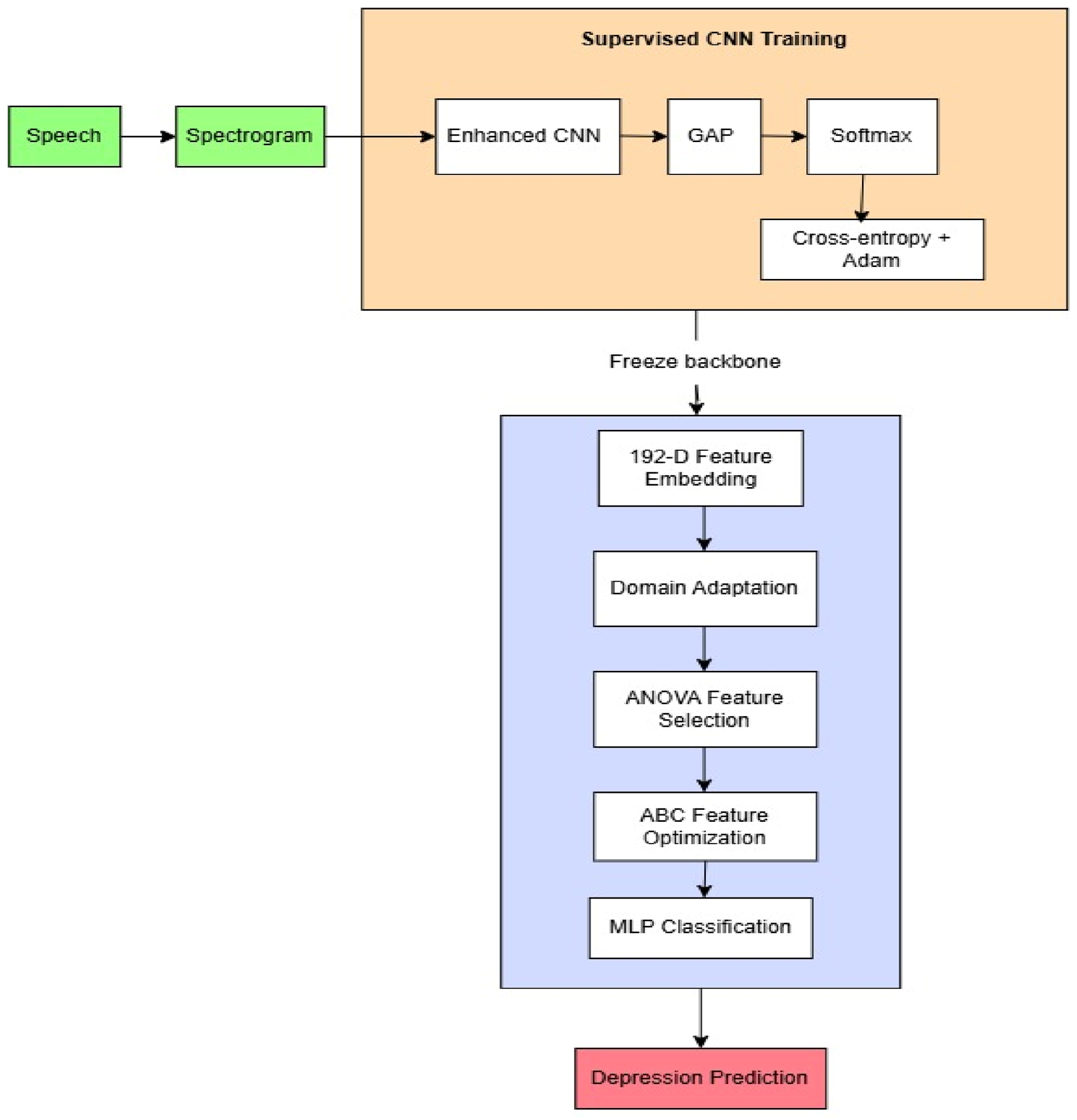
The second enhancement is the adjoining of a Softmax classification head. The CNN is trained on TRAIN data. Based on the classification losses, the layers are also properly updated through backpropagation, thus minimizing the cross-entropy losses. After training, a feature extractor now refines to a discriminative feature extractor when the classification head is removed. This frozen CNN backbone performs task-specific feature extraction with shift invariance provided by Global Average Pooling (GAP) as shown in (6).

After GAP,

$$z \in {\mathbb{R}}^{192}$$

(6)

The classification head computes $p_k$ which is the probability of class k (k = 3 classes).

Further, a two-stage feature selection including ANOVA and ABC optimization is applied followed by final classification by the MLP classifier. The complete workflow is shown in Figure 1.

3.3. Domain Adaptation

Before the process of feature selection begins, a domain adaptation is performed. A lightweight domain-specific feature normalization attempts to alleviate the effect of merging heterogeneous datasets. It normalizes the dataset-specific differences in the combined dataset to be compatible with the shared model. The following Formula (7) is used for the same:

$${\tilde{x}}_d= {\displaystyle \frac{x_d- {\mu }_d}{{\sigma }_d- ϵ}}$$

(7)

where

• $d$ is domain;
• ${\mu }_d$ is mean of domain $d$;
• ${\sigma }_d$ is standard deviation of domain $d$.

The separate normalization of features of each dataset fabricates them to be statistically indistinguishable for the feature selector. This makes each dataset independent of the scale of their raw CNN after concatenation. However, domain-specific feature normalization is not used as inference because, at the deployment level, the objective of detecting depression of any real-world speech and not specifically from the datasets used during training remains. The domain-specific normalization requires information about the domain, but this information will not be available with the arbitrary real-world user recording. Hence, at inference, domain-specific normalization is not applied.

3.4. Feature Selection

Feature selection is an important step for reducing redundant and less significant features from the entire feature space. To ensure only informative feature representation is selected out of all the depression-related information extracted by the trained CNN, a two-step feature selector is used, i.e., Analysis of Variance (ANOVA) and artificial bee colony (ABC) optimization.

The Analysis of Variance (ANOVA) is a statistical method of determining the significance of each extracted feature. It tests the discriminative capability of the feature extracted by the CNN for three levels of depression, that is, healthy, moderate depression, and severe. In this method, an F-score is calculated as the ratio of between-class variance and the within-class variance. Features that have a p-value < 0.05 are called significant features. This p-value is a concerted value of the F-score that is calculated using the F-distribution. The higher the F-score, the lower the p-value and hence the greater the significance of the feature as computed using (8).

$$F={\displaystyle \frac{\mathit{Between}\mathit{class}\mathit{variance}}{\mathit{Within}\mathit{class}\mathit{variance}}}$$

(8)

The next step is artificial bee colony (ABC) optimization. This step was required for considering interactions among multiple features and selecting the optimum feature of the subset through iterative exploration and exploitation. This eventually leads to balance between discrimination capability and computational efficiency as computed using (9).

$$fitness=1-accuracy$$

(9)

These two stages ensure the feature is significant both statistically and optimally. A reduction in weak features reduces the computation burden of the model without losing any important feature.

3.5. Multi-Layer Perceptron (MLP) Classification

After the enriched feature extraction and efficient feature selection which provided a low-dimensional yet highly discriminative feature set, the final step is classification by using the Multi-Layer Perceptron (MLP) classifier. For selected features “$y$”, the MLP can be stated as

$$y=f\left(Wx+b\right)$$

(10)

where

• $W=\mathrm{weight}\mathrm{matrix}$;
• $b=$ bias;
• $f$ = activation function.

An MLP with a single hidden layer with 100 neurons is applied for final classification of severity of depression into three classes for the combined dataset and 4 classes of the EATD separately. With a limited clinical dataset, such a shallow configuration of a dense classifier aids in lessening the overfitting. The lightweight MLP is able to classify complex non-linear decision boundaries efficiently and also generates continuous class-membership probabilities. Later, for examining the reliability of estimated confidence, these probabilities are evaluated using various calibration methods.

3.6. Probability Calibration

The process for re-calculating the confidence score from a model is called probability calibration. It is done in order to reflect the true probability. If a model predicts an 80% chance of the event, it should actually occur 80% of the time.

• If predicted probability > actual probability, then the model is said to be over-confident.
• If predicted probability < actual probability, then the model is said to be under-confident.

For sectors where the probability drives a decision, such as healthcare, the calibration becomes crucial. However, the wrong calibration has limited effect on the accuracy of the model, but for the correct interpretation of the model by the healthcare personnel, it is crucial to calibrate the model. Wrong confidence can mislead healthcare professionals towards misjudgment of diagnosis. The healthcare support systems must be trustworthy enough to help clinicians rather than mislead them. Hence, for increasing trust in the framework at the clinical level, calibration becomes an important part of the framework.

For this process, the calibration technique is applied on the probabilities generated by the Multi-Layer Perceptron (MLP). A calibration compares the predicted and actual probability and finds a correlation. These correlations are learned differently by different calibration methods, and finally, calculations are made to show the actual reliability of the model. In this paper, seven calibration techniques such as Temperature scaling, Platt scaling (Sigmoid calibration), Isotonic regression, Vector scaling, Matrix scaling, Dirichlet calibration and Beta calibration are applied to the framework.

3.6.1. Temperature Scaling

In this calibration method, a positive scalar, Temperature ($T$), is calculated by following the formula as shown in (11):

$$P_i= {\displaystyle \frac{\exp \left(g_i/T\right)}{{\sum }_{j=1}^K\exp \left(g_j/T\right)}}$$

(11)

where

• $P_i$ is predicted logic;
• $K$ is number of classes;
• $g_i$ is logit for class $i$.
• If $T=1$, then original probabilities are not changed.
• If $T>1$, then over-confident predictions are softened.
• If $T<1$, then under-confident predictions are sharpened.

3.6.2. Platt Scaling

This method was developed particularly for SVM and later enhanced for multiclass classifiers. The calibrated probability per class can be calculated as (12):

$$P \left(y=1|x\right)= {\displaystyle \frac{1}{1+\exp (Af\left(x\right)+B)}}$$

(12)

where

• $f\left(x\right)$ is classifier output before calibration.
• $A$ and $B$ are calculated by minimizing the NLL over the calibration data.

3.6.3. Isotonic Regression

This calibration can be calculated using (13):

$$P \left(y=1|x\right)=k\left(f\left(x\right)\right)$$

(13)

where

• $k$(.) is constant monotonic function.

It is suitable for large datasets and overfits for small datasets.

3.6.4. Vector Scaling

It is an extended version of Temperature scaling where an individual scaling coefficient is used instead of a global temperature.

The calibrated logic is given by (14),

$$k^{\prime }=Wk+b$$

(14)

where

• $W$ is diagonal scaling matrix;
• $b$ is bias vector.

The calibrated probability ($P_i)$ is then calculated using (15):

$$P_i= {\displaystyle \frac{\exp \left(k_i^{\prime }\right)}{{\sum }_{j=1}^K\exp \left(k_j^{\prime }\right)}}$$

(15)

3.6.5. Matrix Scaling

This calibration method is a generalized version of Vector scaling. Here, the diagonal scaling matrix is replaced by linear transformation. The probabilities are calculated using the same formula as in Vector scaling except that $W$ becomes a full weight matrix (16),

$$W\in R^{KXK}$$

(16)

And the bias vector becomes (17)

$$b\in R^K$$

(17)

3.6.6. Dirichlet Calibration

This method uses Dirichlet distribution for directly modeling an entire probability simplex as it is designed for multi-class probability calibration. Mathematically calibrated probability is calculated using (18),

$$P^{\prime }=Softmax (Wlog\left(P\right)+b)$$

(18)

where

• $P$ is original probability;
• $W$ is transformation matrix;
• $b$ is bias vector.

3.6.7. Beta Calibration

This calibration uses Beta probability distribution for calculating calibrated probabilities. For binary classification, the following formula is used; however, for multiclass classification, a one-versus-rest (OVR) strategy was used as in (19):

$$P \left(y=1|x\right)= {\displaystyle \frac{1}{1+\mathrm{e}\mathrm{x}\mathrm{p}(a\log \left(p\right)-b\log \left(1-p\right)+c)}}$$

(19)

The calibration method that provides the best accuracy–ECE trade-off is selected for the final saving of the model.

3.7. Reliability Estimation

The above calibrated confidence score is further used for reliability estimation. The method used for this is a fixed-weight combination of bin-based reliability (0.7) and entropy (0.3). A Calibration Lookup table is generated and saved after applying Bayesian smoothing on the bin accuracies. The table consists of bin ranges, smoothed accuracy and number of samples, n. It will be used at the web-based app’s inference for estimating reliability of the depression severity result of the patients’ uploaded speech.

The bin accuracy method firstly divides the confidence score in a particular bin, and then for that bin, smooth accuracy is calculated using the following Formula (20) of Bayesian smoothing:

$$A_{smooth}={\displaystyle \frac{nA+k{A}_0}{n+k}}$$

(20)

where

• $n$ = number of samples;
• $A$ = bin accuracy;
• $A_0$ = prior accuracy = 0.5;
• $k$= prior weight = 10.

This method was incorporated after investigating various techniques for reliability estimation, such as bin accuracy, entropy, weighted combination of bin accuracy and entropy and the Adaptive Reliability Score (ARS). The problem that was aimed to solve is the situation where there are very few samples in a bin. This usually happens in the case of very high confidence or very low confidence bins, and such estimation can be incorrect. Entropy, which is already a well-established uncertainty proxy, does not depend on the sample size and is based on the probability distribution of the current prediction. Hence, a combination of a population-level signal and an instance-level signal (0.7 bin accuracy + 0.3 entropy) is attempted, where the bin accuracy is prioritized along with the learnings of entropy.

However, the fixed weightage of the bin accuracy and entropy does not consider the number of samples present in the bin. The weightage of the bin accuracy of 100 samples and 5 samples cannot be given same. Therefore, an Adaptive Reliability Score (ASR) is investigated. The ARS applies the following formula for determining the weight of both components:

$$\alpha \left(n\right)= {\displaystyle \frac{n}{n+k}}$$

(21)

where

• $n$ = samples present in the bin;
• $k$= prior weight = 10.

If n >> k, then $\alpha \left(n\right)$  approaches 1, and bin accuracy gets prioritized.

If n << k, then $\alpha \left(n\right)$  approaches 0, and entropy gets prioritized which is not dependent on the historical samples.

For testing the above concept, a detailed evaluation and ablation study is discussed in the Results and Discussion Section which could not prove its superiority.

During training phase, the following data are also saved and will be later utilized by the application during the inference phase:

• Trained CNN backbone.
• Scaler.
• ANOVA indices.
• ABC indices.
• Raw model.
• Best calibration method.
• Reliability Lookup Table.

This significantly reduces the computational overhead and processing time required for each audio submission through the web interface.

4. Web-Based Screening System for Depression and PTSD

Another crucial contribution in this paper is a web-based screening system for depression and PTSD. The PTSD detection uses another model that is not in the scope of this paper. The presented work only focuses on the detection model for depression and the deployment of the model as a web-based screening system for speech analysis and detection of depression severity along with confidence of detection for users through a simple browser. It also provides recommendations and informs why this prediction is made through a novel explainability module named pipeline-aware gradient-weighted class activation mapping (PA-Grad-CAM).

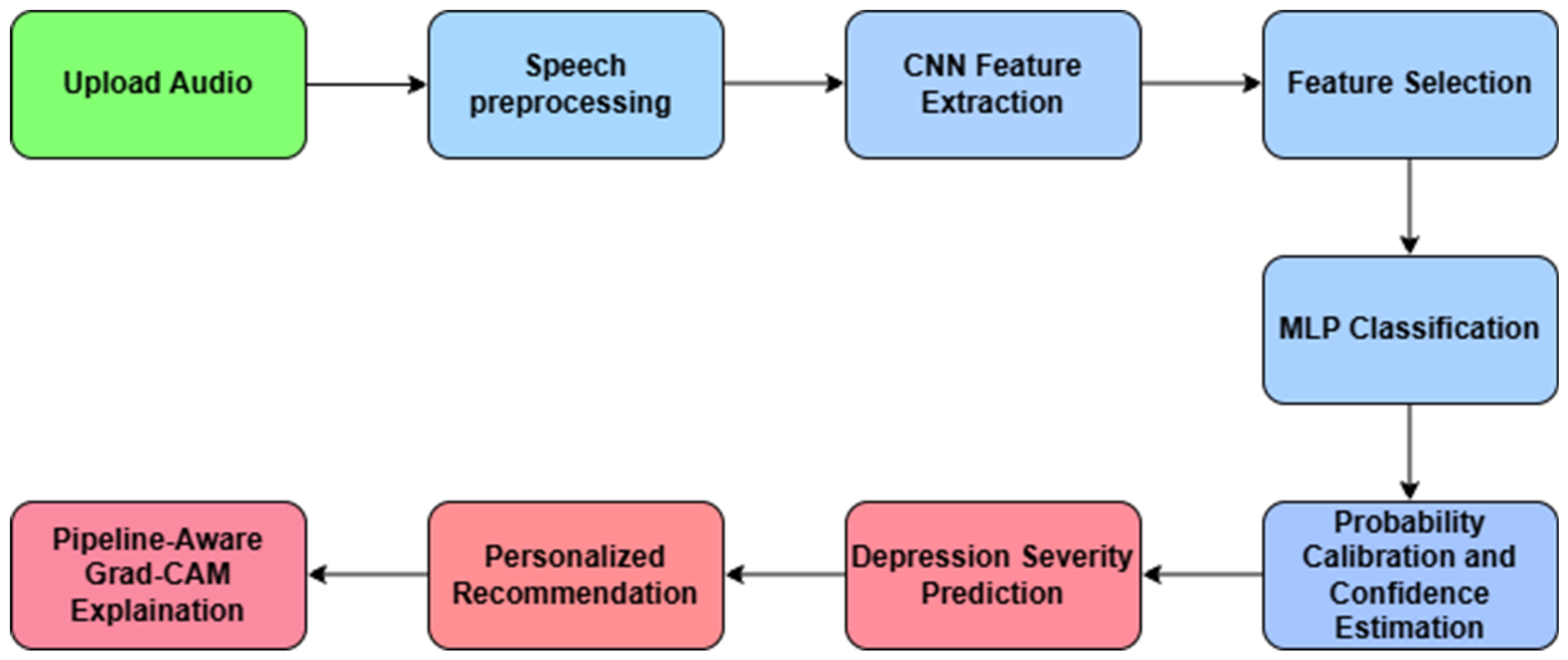
This web-based AI-powered screening system for depression and PTSD is named MindVoice. It uses only inference and skips the computational cost of retraining every time the input is given. The trained and validated model is only loaded once into memory at the beginning of the application. Following is the workflow of MindVoice, shown in Figure 2.

As shown in Figure 2, the audio is uploaded or directly recorded on the web by the user as the first step for depression detection using speech. The audio preprocessing module of the web-based app applies a series of processes such as short-time fourier transform (STFT), decibel-scale representation, z-score normalization and re-sizing of the spectrogram to 64 × 64 on the audio, which is following the same process as during model development.

The model inference module implements the prediction pipeline. A learned CNN feature extractor based on a trained CNN enhanced with Multi-scale and Squeeze-Excitation is used to capture both high-level and low-level features that capture both coarse and fine-grained discriminative acoustic characteristics. This CNN feature extractor is named Frozen CNN backbone. After normalization, only significant features are selected by using the two-stage feature selection. Stage 1 (ANOVA) selects statistically significant features that carry high discriminative capacity, and the remaining features are selected by the ABC optimizer that considers the interaction among the features and selects the optimum features. The final classification into severity classes is done by the Multi-Layer Perceptron (MLP) classifier by calculating the probability of each depression severity class. By using the best calibration method selected during training, this calculated probability is also used to calibrate the confidence score.

Besides reflecting depression severity categories such as Low, Moderate, or High, MindVoice implements four more functions:

• Confidence score that is basically the calibrated confidence reported after calibration.
• Reliability estimation of each prediction for increasing the trustworthiness of the application.
• Recommendation module that provides personalized guidance as per the severity category of depression.
• Explainability module that encourages decision transparency. The explainability module is built on the proposed Pipeline-Aware GradCAM (PA_GradCAM).

4.1. Confidence Score

Once the calibration re-calculates the probability, the probability associated with the predicted class (maximum probability) is assigned as the confidence score displayed in the web-based app MindVoice. This tells how certain the model thinks it is.

4.2. Reliability Estimation

Reliability estimation is done and displayed so that clinicians can know if they can trust the reported confidence or not. The method selected for reliability estimation is a fixed-weight combination of bin-based reliability (0.7) and entropy (0.3). At the inference, the confidence score is calculated by using the calibration method selected during training. Every score is mapped to the Calibration Lookup table, and the reliability score is displayed which is not derived from the confidence score only but also depends upon historical correctness.

4.3. Recommendation Module

It is a lightweight rule-based module that provides predefined recommendations depending upon the level of severity of depression predicted by the model. For a Low level of depression, a healthy lifestyle such as proper sleep, healthy diet, exercise and increasing social interactions is suggested. For a Moderate level of depression, users are suggested to talk openly to family and friends and apply certain stress-management techniques in daily life. For the High level of depression, immediate consultation with a psychiatrist is suggested. Along with this, continuous monitoring is suggested for all levels of depression. This module uses negligible computation and hence provides immediate assistance, increasing the utility of app.

4.4. Explainability Module

The purpose of the explainability module is to provide the reason behind the prediction. This transparency enhances the trustworthiness of the system. A common and efficient method of doing this is by using gradient-weighted class activation mapping (Grad-CAM). However, the existing works of GradCAM that are applicable on the CNN only and other extensions of GradCAM focus on a combination of a CNN and other techniques belonging to the same deep learning framework. The proposed PA-GradCAM bridges the Deep CNN and Classical ML pipeline that includes the Standard scaler + ANOVA + ABC + sklearn MLP. Hence, a novel enhancement of Grad-CAM named pipeline-aware gradient-weighted class activation mapping (PA-GradCAM) is proposed for solving this problem.

The backpropagation from the final classification score to the CNN’s convolutional feature maps is enabled in this hybrid architecture by reconstructing a complete pipeline in a differentiable form. Further, the decision of the deployed model is explained by the heatmap.

4.4.1. PA-Grad-CAM Generation

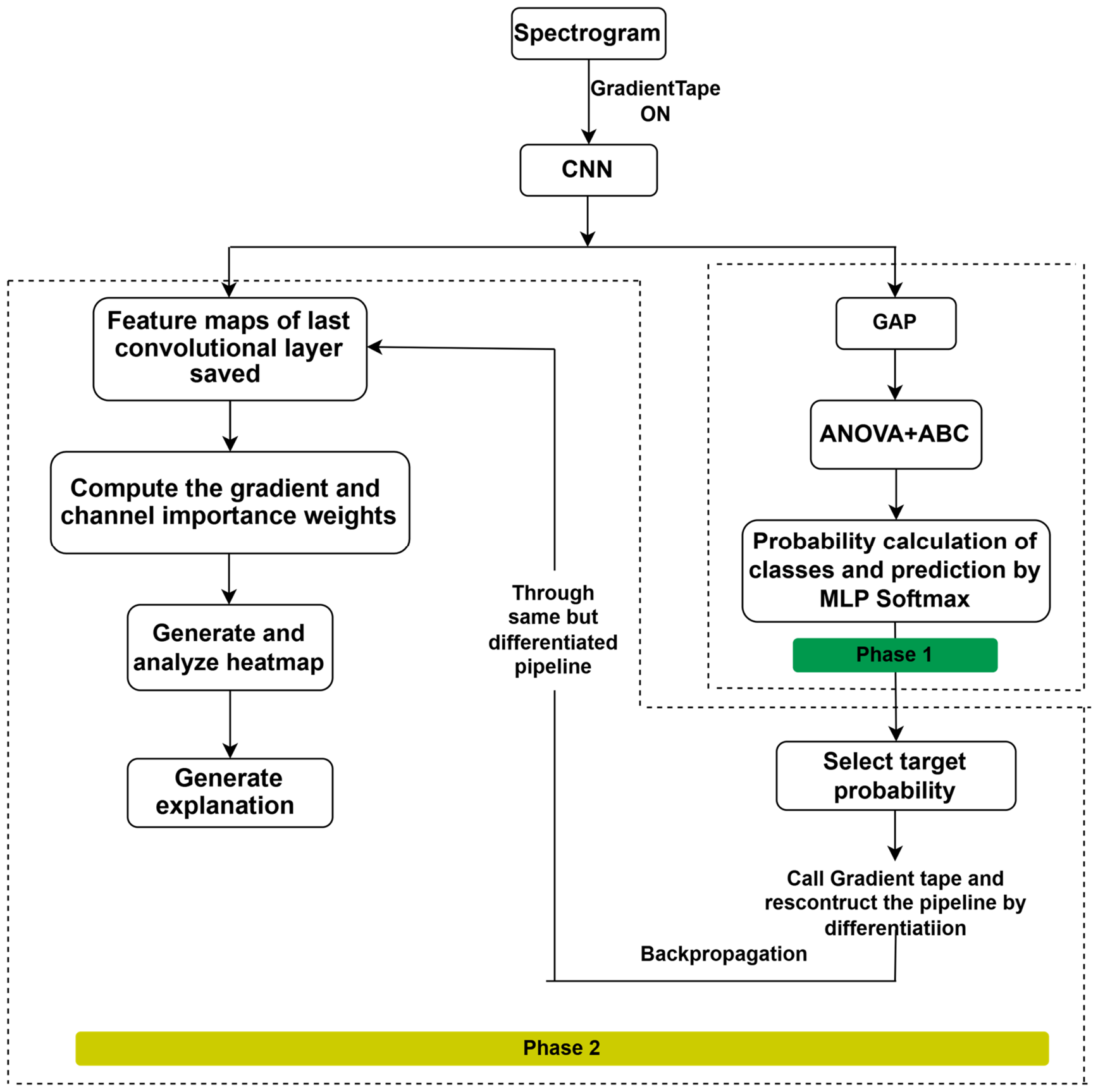
The PA-GradCAM process is applied after the training process. It is divided into two phases: Phase 1: Forward prediction inference, and Phase 2: Backward explanation as shown in Figure 3:

The following Algorithm 1 summarizes the two phases of PA-GradCAM:

Algorithm 1. Pipeline-Aware Grad-CAM (PA-GradCAM)

Phase 1: Forward Prediction Inference Input: Normalized and resized speech spectrogram. Gradient tape starts recording every differentiable operation. Pass spectrogram through the frozen CNN backbone. Save the last convolutional feature maps to be used by Grad-CAM. Apply Global average pooling (GAP) for one-dimensional feature vector calculation. Normalization of feature vector using Standard scaler parameters stored during training phase. First stage of feature selection based on statistics using stored ANOVA indices. Second stage of feature selection based on optimization using stored ABC indices. Selected features are applied to trained MLP classifier. Class probabilities are calculated by Softmax. Select the probability score of predicted class. Phase 2: Backward Explanation Reconstruct the Standard scaler as Tensorflow subtraction and division using the stored mean and standard deviation. Reconstruct the trained sklearn MLP using TensorFlow matrix multiplication, bias addition, activation functions and Softmax with the stored weights. Replace ANOVA and ABC feature selection by TensorFlow gather operations using the stored feature indices. Back-propagate through reconstructed pipeline inside TensorFlow Gradient tape. Using saved last convolutional feature map, compute the gradient of the selected probability score. Compute channel importance weights. Generate and normalize and resize the heatmap. Analyze the heatmap and determine dominant time region, dominant frequency region and attention concentration. Generate explanation with the calibrated confidence score.

The depression detection inference pipeline is not differentiable as they are implemented using scikit-learn components and saved fixed indices except the CNN and GAP. Gradients cannot backpropagate through a pipeline whose components exist outside the automatic differentiation framework of TensorFlow. The proposed PA-GradCAM resolves this problem by reconstructing the pipeline in the form of Tensorflow. The mathematical equivalents of the sklearn components as the Tensorflow components are as follows:

Let the feature vector generated by GAP be (22),

$$z \in {\mathbb{R}}^{192}$$

(22)

and then the reconstruction stages after GAP are as follows:

• Standard Scaler Reconstruction:

The Standard scaler standardizes the feature vector generated by GAP, and in the process, it saves the mean ($\mu$) and standard deviation ($\sigma$) of the feature. Since scaling was performed by the scikit-learn object, it is not differentiable; PA-GradCAM reconstructs by utilizing those mean and standard deviations and makes it differentiable as given by (23):

$$\widehat{z}= {\displaystyle \frac{z - \mu }{\sigma }}$$

(23)

2.

ANOVA and ABC Reconstruction:

Once the training is complete, the ANOVA-selected and ABC-selected feature indices are saved. At this stage, the indices remain fixed at inference, so the PA-GradCAM reconstructs by using Tensorflow’s gather operation (24) and (25):

$$z_A=gather (ANOVA Indices)$$

(24)

$$z_B=gather (ABC Indices)$$

(25)

3.

MLP Reconstruction:

The MLP classifier is a trained sklearn; hence, it needs to be reconstructed. If $y$ is the selected feature, each hidden layer is stated as (26):

$$y=f\left(Wx+b\right)$$

(26)

where

• $W=\mathrm{weight}\mathrm{matrix}$;
• $b=$ bias;
• $f$ = activation function.

The final layer computes logits as (27):

$$h=\left(Wx+b\right)$$

(27)

Softmax is defined as (28):

$$P\left(c\right)={\displaystyle \frac{\exp \left(l_c\right)}{{\displaystyle {\sum }_{k=1}^C}\exp \left(l_k\right)}}$$

(28)

where

• $P\left(c\right)$ = probability of class $c$;
• $l_c$ = logit of class $c$;
• $l_k$ = logits of all classes.

This reconstructed pipeline aids in the backpropagation of the gradient up to the saved feature maps of the last convolution layer. Then, the standard Grad-CAM comes into action and performs the channel importance weight calculation from the obtained gradients and generates the heatmap.

4.4.2. Heatmap-to-Text Interpretation

For generating the textual explanation behind the prediction, the following task-specific interpretation interface is applied:

Input: Normalized PA-Grad-CAM heatmap

• Calculate temporal and frequency attributions.
• Locate their maximum positions.
• Normalize peak positions to [0, 1].
• Calculate the heatmap concentration and active-region fraction.
• Categorize attribution as localized or distributed attributes.
• Map with pre-written text templates.

If the normalized heatmap is taken as (29):

$$H\in {\left[0, 1\right]}^{H\times W}$$

(29)

where

• $H$ is number of frequency;
• $W$ is number of time.
• Let $H_{f,t}$ be the heatmap at frequency f and time t.

• The time-wise importance profile is given by (30):

$$T_t={\displaystyle \frac{1}{H}}{\displaystyle {\sum }_{f=1}^H}{H}_{f,t}$$

(30)

The model attributes high importance to that temporal region where the time position has a large $T_t$.

2.

The frequency-wise importance profile is given by (31):

$$F_f={\displaystyle \frac{1}{W}}{\displaystyle {\sum }_{t=1}^W}{H}_{f,t}$$

(31)

The model attributes high importance to that frequency region where the frequency position has a large $F_f$.

3.

Temporal peak:

$$t^{*}=\mathit{arg}\underset{t}{\max } T_t$$

(32)

The normalized temporal location is

$$P_t={\displaystyle \frac{t^{*}}{\max (W-\mathrm{1,1})}}$$

(33)

4.

Frequency peak:

$$f^{*}=arg \underset{f}{\max } F_f$$

(34)

The normalized location is

$$P_f={\displaystyle \frac{f^{*}}{\max (H-\mathrm{1,1})}}$$

(35)

5.

Concentration of the heatmap is given by (35),

$$C=\sqrt{{\displaystyle \frac{1}{HW}}{\displaystyle {\sum }_{f=1}^H}{\displaystyle {\sum }_{t=1}^W}{\left(H_{f,t}-\overline{H}\right)}^2}$$

(36)

Large $C$ shows that attribution values vary more strongly across the spectrogram.

Smaller $C$ shows that attribution values are homogeneous across the spectrogram.

6.

For checking localization, the Active fraction is utilized as (37):

$$A={\displaystyle \frac{1}{HW}}{\displaystyle {\sum }_{f=1}^H}{\displaystyle {\sum }_{t=1}^W}1\left(H_{f,t}>0.5\right)$$

(37)

7.

According to the predefined heuristic threshold,

If $C$ > 0.20 and $A$ < 0.25 ⇒ high concentration + small active area ⇒ localized attribution.

If $C$ ≤ 0.20 or $A$ ≥ 0.25 ⇒ low concentration + big active area ⇒ distributed attribution.

8.

Lastly, predefined text templets are mapped.

4.4.3. PA-Grad-CAM Validation Protocol

For the validation of PA-Grad-CAM explanations, we performed three experiments:

• Prediction Equivalence;
• Gradient Correctness;
• Perturbation-Based Faithfulness.

Prediction Equivalence

It is based on the implementation-invariance principle described by Sundararajan et al. [45]. For examining if both the trained pipeline and the reconstructed pipeline are generating equivalent prediction, predictions are generated for the test set on both the trained and reconstructed pipeline. It then compares the final predictions. If prediction of the trained pipeline and the reconstructed pipeline are same, then the reconstruction pipeline is successfully established to be equivalent to the trained pipeline.

Gradient Correctness

It is based on the gradient-checking principle proposed by Ben-Nun et al. [46]. For 20 test samples, Analytical gradients as well as Numerical gradients are calculated. The Analytical gradients are obtained using Gradient tape and the Numerical gradients are obtained using (38) as follows:

$$g_{numerical}= {\displaystyle \frac{f\left(x+ϵ\right)-f(x-ϵ)}{2ϵ}}$$

(38)

Comparing these two gradients provides proof regarding the correctness of gradient propagation through the reconstructed pipeline.

If the Pearson correlation ≥ 0.99 and median error ≤ 0.05, then the gradient propagation is correct. Also, for finding a numerically stable region, four values of $ϵ$ are tested.

Perturbation-Based Faithfulness

For checking if regions highlighted by PA-GradCAM actually matter, perturbing the spectrogram is implemented through two processes called deletion and insertion as first proposed by Petsiuk, V et al. [47]. The process of deletion gradually decreases the important region of PA-GradCAM. For a faithful system, the probability of prediction will drop if its important regions are deleted. Similarly, for a faithful system, inserting important regions increases the probability of prediction quickly. On the test dataset, the Deletion AUC, Insertion AUC, difference/advantage over random and Paired t-test is calculated.

5. Results and Discussion

5.1. Performance of the Proposed Framework

The proposed framework utilizes four datasets, DAIC, EDAIC, MODMA and EATD, and classifies them into three classes, Low, Moderate and High levels of depression, for the DAIC, EDAIC, MODMA and into four classes for the EATD. Three types of experiments are conducted for results: first is analysis on the combined dataset, second is the analysis of individual test datasets while being trained on a combined dataset and analysis on the EATD, and last is the leave-one-dataset-out (LODO) evaluation.

5.1.1. Combined Dataset Analysis

For the framework, when applied to the combined dataset, an accuracy of 76.5% is achieved without calibration. The analysis also includes other metrics such as precision, recall and F1 score that are mathematically defined as below and provides an average of the precision, recall and F1 score as 76.5% as given through (39) to (42). The class wise precision, recall and F1 score are provided in

Table 4. Classification report for precision, recall and F1 score for three-class classification (EATD excluded).

Class	Precision	Recall	F1 Score
Low	0.695	0.680	0.688
Moderate	0.772	0.723	0.747
High	0.823	0.893	0.857

.

$$Accuracy={\displaystyle \frac{TP+TN}{TP+FP+TN+FN}}$$

(39)

$$Precision={\displaystyle \frac{TP}{TP+FP}}$$

(40)

$$Recall={\displaystyle \frac{TP}{TP+FN}}$$

(41)

$$F1 Score=2·{\displaystyle \frac{Precision · Recall}{Precision+Recall}}$$

(42)

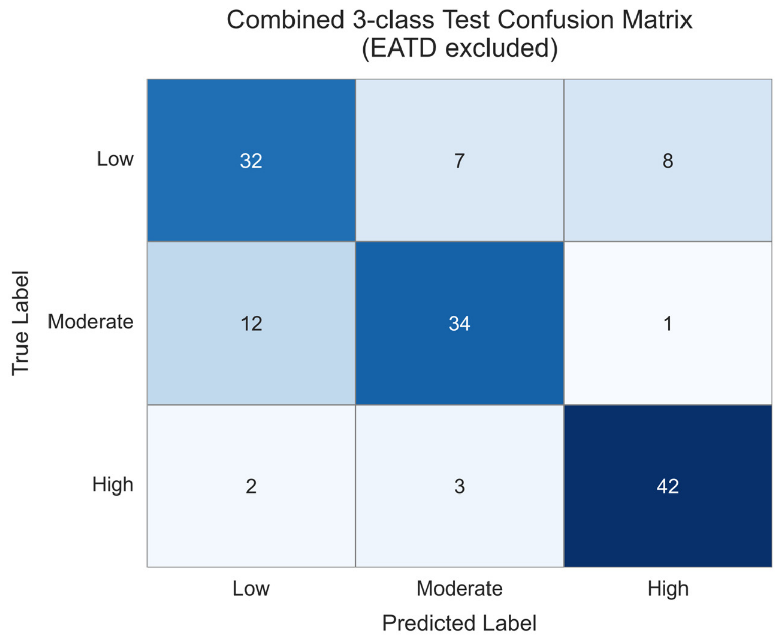
Figure 4 shows the Confusion Matrix (EATD excluded) that represents correct prediction by dark color diagonal elements and incorrect prediction by light color non-diagonal elements.

5.1.2. Individual Dataset Performance

The performance of an individual dataset is calculated by accuracy, along with metrics such as the Expected calibration error (ECE), Negative log-likelihood (NLL) and Brier score.

Expected calibration error (ECE) is defined as the difference between the classification accuracy of the $m^{th}$ confidence bin and predicted confidence of those samples. The lower the ECE value, the better the calibration of the model, the lesser the difference between the predicted confidence and actual confidence. It can be mathematically defined as (43):

$$ECE={\displaystyle {\sum }_{m=1}^M}{\displaystyle \frac{\left|B_m\right|}{N}}\left|acc\left(B_m\right)-conf\left(B_m\right)\right|$$

(43)

where

• $B_m$ is set of predictions of $m^{th}$ confidence bin;
• $\left|B_m\right|$ is number of samples in bin;
• $N$ is total test sample;
• $acc \left(B_m\right)$ = classification accuracy of samples;
• $conf \left(B_m\right)$ is average predicted confidence.

Negative log-likelihood (NLL) can be defined as a qualitative metric that evaluates both the accuracy and confidence of the prediction. The lower the NLL value, the better the probabilistic confidence. Mathematically:

$$NLL=-{\displaystyle \frac{1}{N}}{\displaystyle {\sum }_{i=1}^N}\log P\left(y_i\right|x_i)$$

(44)

where;

• $P$ ($y_i| x_i$) is predicted probability;
• $N$ is total test sample.

The Brier score is defined as the measurement of the accuracy of predicted probabilities of all defined classes. Mathematically, it can be stated as (45):

$$BS={\displaystyle \frac{1}{N}}{\displaystyle {\sum }_{i=1}^N}{\displaystyle {\sum }_{k=1}^K}{(p_{ik}-y_{ik})}^2$$

(45)

where

• $N$ is total number of samples;
• $K$ is number of classes;
• $p_{ik}$ is predicted probability;
• $y_{ik}$ is true label.

Table 5. Accuracy, AUC, ECE, Brier score and NLL for both combined dataset and individual datasets.

Dataset	N	Accuracy	AUC	ECE	Brier Score	NLL
DAIC	54	0.814	0.948	0.159	0.317	0.971
E-DAIC	72	0.722	0.893	0.229	0.474	1.348
MODMA	15	0.80	0.84	0.178	0.370	1.911
Combined	141	0.765	0.906	0.190	0.403	1.263

shows all the above stated metrics along with the number of samples, accuracy and AUC. The accuracy is quite stable for all the individual datasets without calibration. It ranges from 72.2% for the E-DAIC to 81.4% for the DAIC, while MODMA achieved 80% accuracy.

Table 6. Accuracy, AUC, ECE, Brier score and NLL for EATD datasets.

Dataset	N	Accuracy	AUC	ECE	Brier Score	NLL
EATD	39	0.785	0.972	0.159	0.116	0.518

shows the evaluation of the EATD test data and achieves an accuracy of 78.5%. The accuracy across all four datasets under different experimental setups implies consistent applicability of the proposed framework across used datasets. The accuracy of the combined data which includes three datasets (DAIC, E-DAIC and MODMA) is 76.5% which shows that the model is able to extract useful features and finally classify with reasonable accuracy despite heterogeneity.

5.1.3. Leave-One-Dataset-Out (LODO) Evaluation

In the combined dataset experiment, the test split of each dataset was strictly held out and never used during training or validation. However, this does not represent absolutely unseen data. For evaluating unseen data, the leave-one-dataset-out (LODO) evaluation method is used. In this, a target dataset is kept completely absent from the training dataset. Its purpose is the investigation of the efficiency of the trained model in transferring the learnings. In this study, two datasets out of three datasets (DAIC, E-DAIC and MODMA) are considered for training and the remaining dataset for testing.

Table 7. Accuracy, AUC, ECE, Brier score and NLL for leave-one-dataset-out (LODO) evaluation.

Held Out Dataset	Training Datasets	Accuracy	AUC	ECE	Brier Score	NLL
DAIC	E-DAIC + MODMA	0.777	0.906	0.147	0.330	0.914
E-DAIC	DAIC + MODMA	0.513	0.700	0.351	0.787	2.51
MODMA	DAIC + E-DAIC	0.4	0.706	0.527	1.108	5.77

shows the results for leave-one-dataset-out (LODO) evaluation. The DAIC demonstrated relatively strong transfer (77.7% accuracy and AUC of 0.906) while the E-DAIC (51.3% accuracy and AUC of 0.70) and MODMA (40% accuracy and AUC of 0.706) struggled. These variations in results indicate towards the asymmetric dataset-dependent transferability for an unseen corpus.

5.2. Comparison Among the Calibration Techniques

Different calibration techniques are applied for re-calculating confidence on the validation set.

Table 8. Accuracy, ECE, Brier score and NLL for different calibration techniques.

Method	Accuracy	ECE	Brier Score	NLL
Platt Sigmoid	0.750	0.030	0.409	0.702
Dirichlet Calibration	0.715	0.059	0.400	0.669
Isotonic	0.770	0.061	0.362	0.608
Matrix Scaling	0.715	0.061	0.400	0.669
Vector Scaling	0.680	0.091	0.406	0.688
Beta Calibration	0.722	0.094	0.414	0.704
Temperature Scaling	0.743	0.104	0.417	0.744
Uncalibrated	0.743	0.223	0.478	1.794

shows the number of samples, accuracy, ECE, barrier score and NLL for seven calibration techniques named Platt scaling, Isotonic regression, Temperature scaling, Vector scaling, Matrix scaling, Dirichlet calibration and Beta calibration along with Uncalibrated. Table 8 given below clearly shows that the model is fairly calibrated even without any calibration.

The accuracy does not vary much due to calibration and its value remains stable throughout the experiment with the above calibration techniques. The accuracy varies from 68% (Vector scaling) to 77%, which is achieved by Isotonic regression. Calibration methods secured accuracy with much less fluctuation which indicates that the framework is already stable.

The ECE is best when it is lowest. Platt shows the lowest value of 0.030. The value of the Brier score is also the lowest for Isotonic with a score 0.362. The NLL value is the lowest of 0.608 for Isotonic. The Uncalibrated model showed a reasonable closer value w.r.t to all the metrics.

The Platt is selected as the best calibration method based on the best accuracy–ECE trade-off. This method will be used for the final saving of the model which will be used for inference after deployment of the model on the web.

5.3. Validation of PA-Grad-CAM Explanations

For validation of PA-Grad-CAM explanations, the following three experiments are performed.

5.3.1. Prediction Equivalence

It is used to confirm equivalence of the original pipeline and the reconstructed pipeline.

Table 9. Prediction-equivalence verification.

Model	Dataset(s)	Final Probability Max abs. diff.	Prediction Reproducibility	Result
Combined 3-class PHQ model	DAIC + EDAIC + MODMA	3.46 × 10−6	100%	PASS
EATD 4-class SDS model	EATD	1.50 × 10−6	100%	PASS
Overall	All datasets	3.46 × 10−6	100%	PASS

shows the negligible value of the final probability maximum absolute difference, confirming that the training pipeline is the same as the reconstructed pipeline. The 100% prediction reproducibility proves the Prediction Equivalence in PA-GradCAM.

5.3.2. Gradient Correctness

It is used to check if the gradients obtained through the reconstructed pipeline are correct. For this evaluation, 20 test samples were taken and a total 400 gradient locations were evaluated considering the step size ε = 0.01.

Table 10. Gradient Correctness evaluation.

Metric	Result
Test samples	20
Feature-map locations per sample	20
Total gradient locations evaluated	400
Gradient target	Original predicted-class logit
Analytical gradient	Backpropagation gradient
Numerical gradient	Central finite-difference approximation
Step size, ε	0.01
Mean Pearson correlation	0.999989
Median Pearson correlation	1.000000
Minimum Pearson correlation	0.999812
Mean absolute error	4.34 × 10−5
Median sample-level relative error	1.59 × 10−4
Verification result	PASS

shows all correlation values are either 1 or very close to 1 which implies a very strong positive linear relationship. However, the error values are negligible, verifying that the analytical gradients are correctly implemented in PA-GradCAM.

5.3.3. Perturbation-Based Faithfulness

It is used to observe the fluctuations in the probability of prediction while deleting and inserting important regions.

In

Table 11. Perturbation-based faithfulness (deletion/insertion).

Dataset	Deletion AUC Grad-CAM ↓	Deletion AUC Random ↓	Deletion Advantage ↑	p-Value	Insertion AUC Grad-CAM ↑	Insertion Advantage ↑	p-Value
DAIC	0.4666	0.6116	0.1450	<0.001	0.7437	0.0838	<0.001
EDAIC	0.4056	0.5749	0.1693	<0.001	0.6694	0.0704	0.0014
MODMA	0.3117	0.5734	0.2617	0.0038	0.7004	0.0936	0.0945
EATD	0.3641	0.4782	0.1141	<0.001	0.6727	0.1468	<0.001
All	0.4099	0.5705	0.1606	<0.001	0.6964	0.0894	<0.001

, ↓ shows lower is better and ↑ shows higher is better. Here, both deletion and random deletion shows a reduction in AUC while insertion shows an increase in AUC. Deletion advantage and insertion advantage both show positive values, implying that the model’s confidence drops more rapidly when important regions are removed and PA-GradCAM restores faster when important regions are inserted. This confirms the faithfulness of the PA-GradCAM. However, for MODMA, PA-GradCAM is supporting the faithfulness, while deletion, but for insertion 0.0945 > 0.05, does not show statistical significance. This can be due to the low number of samples in MODMA (15).

5.4. Ablation Study and Baseline Comparison with the Proposed Framework

An evaluation is performed considering four configurations built around two factors: Trained CNN or Untrained CNN and flatten or GAP (Global Average Pooling). Flatten takes every feature produced by the CNN and puts them as a long vector. It is supposed to have all the spatial information but also carries redundant features and has higher computational cost. The GAP in contrast calculates the average of all spatial positions and results in lower redundancy and computational cost. The four configurations are: Untrained CNN + Flatten, Untrained CNN + GAP, and Trained CNN + Flatten and Trained CNN + GAP (Main Pipeline). For flatten in both Trained CNN and Untrained CNN, 12,288 features are generated and only 3600 and 2671 features respectively remain after two-stage feature selection. This clearly shows that flatten carries a larger number of insignificant features. However, the GAP for both Trained CNN and Untrained CNN produces 192 features and only 99 and 67 remain after two-stage feature selection.

The comparison in

Table 12. Comparison between different CNN feature extraction configuration w.r.t. accuracy, ECE, Brier score and NLL.

Configuration	Features Generated	Features After ANOVA	Features After ABC	Accuracy	ECE	Brier Score	NLL
Untrained CNN + Flatten	12,288	5335	2671	0.794	0.091	0.309	0.722
Untrained CNN + GAP	192	145	67	0.737	0.136	0.382	0.797
Trained CNN + Flatten	12,288	7222	3600	0.765	0.184	0.410	1.263
Trained CNN + GAP (Main Pipeline)	192	191	99	0.765	0.190	0.403	1.263

shows that Untrained CNN + Flatten gave the best accuracy among all, but Trained CNN + GAP results in reasonable accuracy despite containing substantially fewer features, which confirms that it contains more discriminative information despite having much fewer features. This would result in lesser computational loads on the system.

5.5. Reliability-Weight Ablation Study

Pearson correlation is computed using the following formula to check if correct predictions can increase the reliability score; the higher the better:

$$r=corr (Reliability Score, Correctness)$$

(46)

where

• Correctness = 1 for correct prediction;
• Correctness = 0 for incorrect prediction.

ROC-AUC measures how well correct and incorrect prediction is distinguished by the reliability score. The Brier score is used to compute the closeness of the reliability score to the actual outcome through the following formula:

$$Brier= {\displaystyle \frac{1}{N}}\sum {(R_i-y_i)}^2$$

(47)

where

• $R_i$ = reliability score;
• $y_i$ = correctness.

As per

Table 13. Ablation table showing Pearson correlation, AUC and Brier Vs correctness for different formulations.

Formulation	Alpha Bin Accuracy	Beta Entropy	Pearson Correlation with Correctness	AUC	Brier Vs Correctness
0.7 bin/0.3 entropy	0.7	0.3	0.450	0.804	0.145
0.6 bin/0.4 entropy	0.6	0.4	0.447	0.800	0.146
0.5 bin/0.5 entropy	0.5	0.5	0.443	0.798	0.148
Adaptive Reliability Score (ARS)	NaN	NaN	0.408	0.797	0.149
Entropy only	NaN	NaN	0.414	0.656751	0.1659
Bin accuracy only	NaN	NaN	0.445	0.674	0.147

, the ARS provided competitive reliability discrimination with AUC 0.797, but the formulation 0.7 bin/0.3 entropy provided the best value for the Pearson correlation with correctness, AUC and Brier Vs correctness and outperformed other formulations. The ARS is part of the investigation and is not claimed as a contribution of this paper.

5.6. Signal Independence Analysis

The two components are further examined to determine whether bin accuracy and entropy contribute distinct information to the reliability estimation. This analysis helps assess whether both components provide complementary rather than redundant information. Two evaluations are carried out for this purpose.

First, Pearson’s correlation coefficient is calculated between bin accuracy and entropy. A lower correlation value suggests that the two measures capture different aspects of the prediction behavior.

In addition, logistic regression is used to investigate the contribution of these two components to reliability estimation. The logistic regression model is formulated as shown in (48):

$$P \left(correct=1\right)= {\displaystyle \frac{1}{1+\exp [-({\beta }_0+{\beta }_{1}B+ {\beta }_{2}E\left)\right]}}$$

(48)

where

• $B$ = bin accuracy;
• $E$ = entropy.

${\beta }_0$ and ${\beta }_1$ are regression estimates that tell one about the amount of information carried by $B$ and $E$ respectively.

A combined AUC is also calculated along with AUC bin-accuracy only and AUC entropy only.

Table 14. Metrics and respective results for estimating independence of information.

Metrics	Results
Pearson r (bin accuracy, entropy)	0.841
AUC—bin-accuracy only	0.674
AUC—entropy only	0.796
AUC—both combined	0.797
Logistic coefficient—bin accuracy	2.315
Logistic coefficient—entropy	2.231

shows the metrics and respective results for estimating independence of information.

The above results conclude that bin accuracy and entropy are substantially correlated and carry redundant information. However, the entropy is still significant when there are not enough samples in the bin to provide significant information. Overall, the proposed ARS could not show its superiority over other formulations, and hence, it is not claimed as a contribution. The analysis was conducted and presented for exploring if it could lead to an interpretable reliability signal.

5.7. Web Application

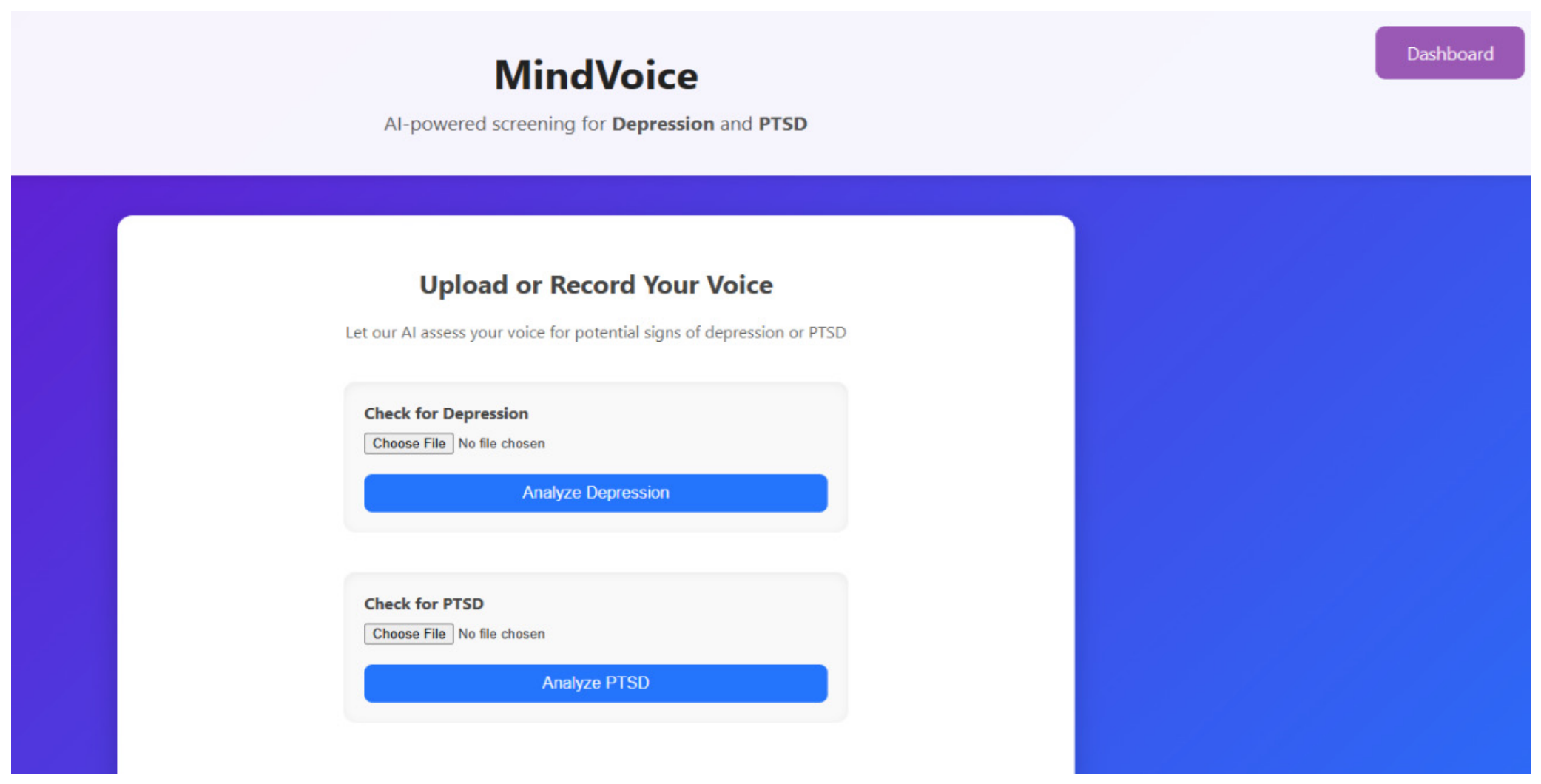
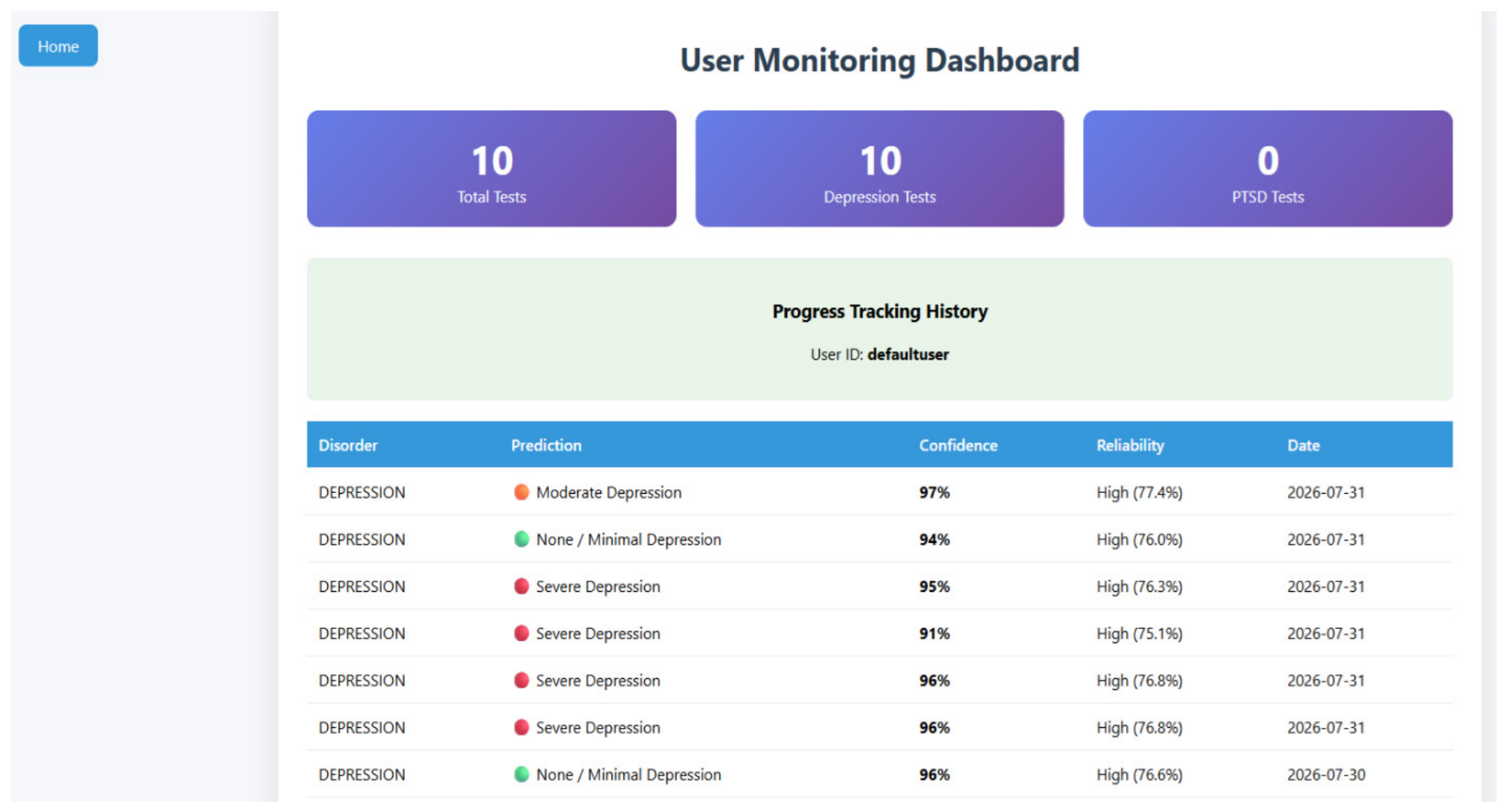
Following are artifacts showing the home page and result page of the web-based application MindVoice. The home page (Figure 5) has the “Upload or Record Your Voice” button separately for depression and PTSD as they use different models. It also has “Dashboard” that shows the trend of the severity level of depression of the user (Figure 6).

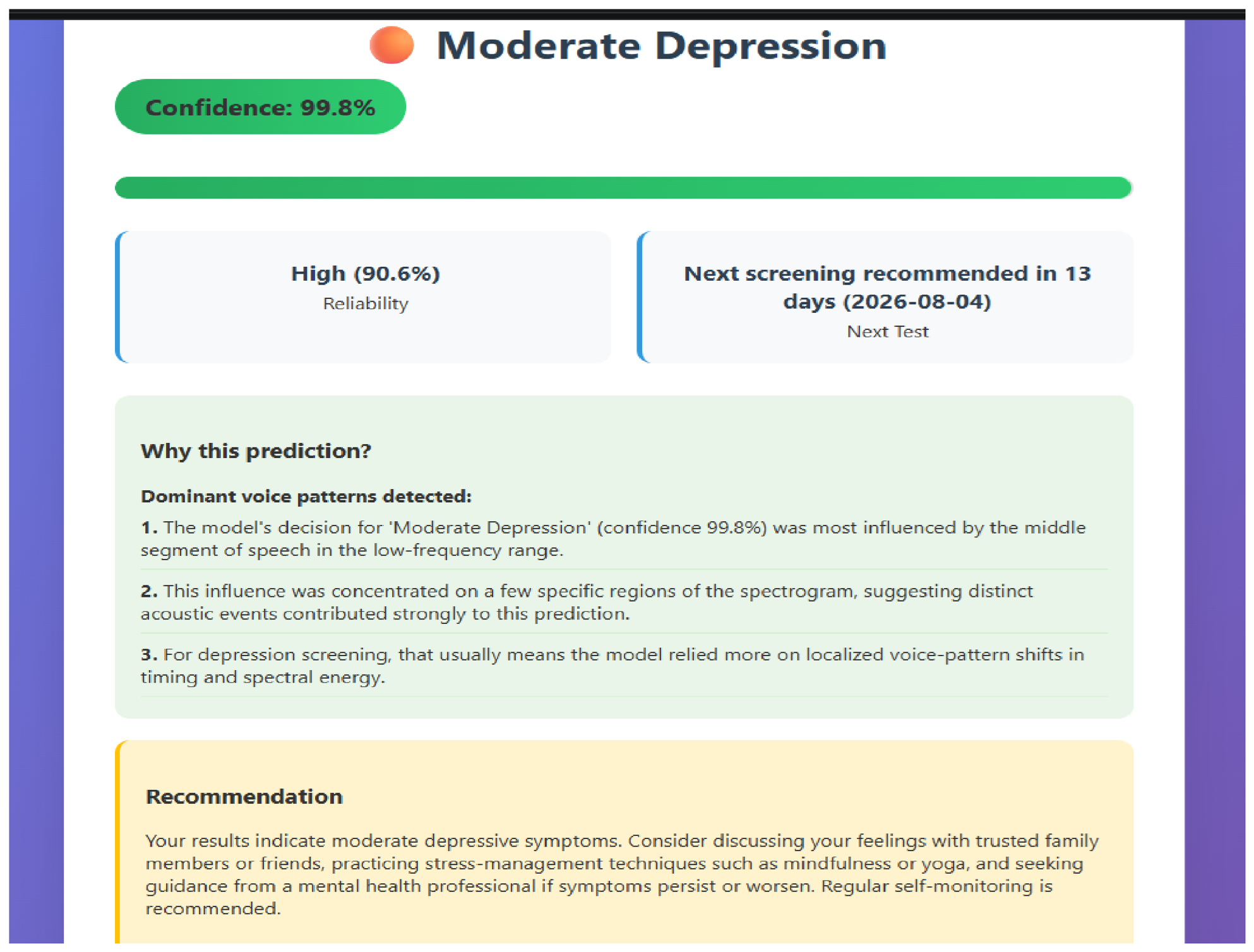
Figure 7 shows the result page. It consists of the following features:

• Level of depression classified as Low, Moderate and High Depression.
• Confidence score.
• Reliability score.
• Next screening day recommendation.
• Why this prediction? Using our proposed PA-GradCAM.
• Recommendations.

5.8. Comparison with Existing Work

A comparison with relevant studies indicates that existing speech-based approaches have predominantly focused on depression detection or screening, while the proposed method specifically addresses three levels of depression severity. DL4DED was developed for depressive episode detection using the DAIC-WOZ dataset and reported an accuracy of 50% [40]. VoiceSense was evaluated as a content-free-speech analysis tool for assessing affective distress in mental health and reported an accuracy of 68% [41]. MoodEcho was developed for automatic depression screening using speech in English and Chinese and reported F1 scores of 86% for English and 75% for Chinese data [42]. In contrast, the proposed approach performs three-level depression severity classification, thereby extending speech-based depression assessment beyond conventional binary detection. Another relevant work used two datasets (DAIC-WOZ and MODMA) and reported the accuracy and AUC score using two evaluation systems, 5-fold cross validation and out-of-fold (OOF) aggregation. Accuracy was 68% and 79% respectively and AUC is 90% and 86% respectively. In comparison to the above works, MindVoice achieved a competitive result despite using three combined datasets (DAIC-WOZ, E-DAIC, and MODMA) for three-level classification and the separate EATD dataset four-level classification as shown in

Table 15. Comparison with existing state-of-the-art models w.r.t. to task, datasets used, accuracy, F1 and AUC.

System	Task	Datasets Used	Accuracy	F1	AUC
DL4DED [48]	Binary Classification	DAIC-WOZ	0.50	-	-
VoiceSense [49]	Binary Classification	DAIC-WOZ + Androids Corpus	0.68	-	-
MoodEcho [50]	Binary Classification	DAIC-WOZ + Chinese clinical-interview dataset	-	English— 0.86 Chinese—0.75	-
Smartphone narratives + WavLM [51]	Binary Classification	DAIC-WOZ + MODMA	5-fold cross val- 0.68 OOF- 0.79	-	5-fold cross val-0.90 OOF-0.86
MindVoice (Proposed)	Multi-class Classification (3 Classes for DAIC-WOZ, E-DAIC, MODMA and 4 Classes for EATD)	DAIC-WOZ, E-DAIC, MODMA, EATD	DAIC-0.814 E-DAIC-0.722 MODMA-0.8 EATD-0.785 Combined-0.765	-	DAIC-0.948 E-DAIC-0.893 MODMA-0.84 EATD-0.972 Combined-0.862

.

In

Table 16. Comparison with existing works regarding confidence, reliability, explanation and generalization.

System	Confidence	Reliability	Explanation	Generalization
DL4DED	No	No	No	No
VoiceSense	Yes	No	Partial (Vocal characteristics/parameters)	Yes (2 datasets)
MoodEcho	Yes	No	No	Yes (2 datasets)
Smartphone narratives + WavLM	Yes	No	No	Yes (2 datasets)
MindVoice (Proposed)	Yes	Yes	Yes (PA-Grad-CAM)	Yes (4 datasets and combined data evaluation)

, a comparison is made with the existing work regarding confidence, reliability, explanation and generalization. Other than confidence, all other modules are not implemented by the existing works. Also, for generalization, a maximum of two datasets were taken into account, whereas MindVoice considers four datasets with both combined evaluation, per-dataset evaluation and leave-one-dataset-out (LODO) evaluation.

6. Conclusions

This paper presents a web-based application “MindVoice” for detecting depression severity as Low depression, Moderate depression and High depression using speech. MindVoice is based on a framework that uses a trained CNN-based feature extractor enhanced by Multi-scale and Squeeze and Excitation mechanisms. Further, a two-stage feature selector is applied, and final classification is done by an MLP classifier and secures an accuracy of 76.5% for the combined dataset.

This work also includes confidence scoring after analyzing various calibration methods, reliability estimation and explainability modules for which a novel Pipeline-Aware Grad-CAM is proposed. The model is evaluated by three experimental setups. First is analysis on the combined dataset (DAIC, E-DAIC, and MODMA), second is the analysis of individual test datasets while being trained on the combined dataset and analysis on the EATD, and last is leave-one-dataset-out (LODO) evaluation. For mitigating the heterogeneity, domain-specific feature normalization is used for domain adaptation. All the above functions are not just implemented in the paper but also integrated for users in MindVoice.

The limitation of this work is the small test set of MODMA and enough dataset heterogeneity due to differences such as language. For future work, a large and diverse dataset can be used with stronger feature representation and domain handling. A multimodal input such as text and visuals can also be integrated for capturing details that only speech cannot capture for severity detection of depression.

References

1. World Health Organization. Depression. Available online: https://www.who.int/news-room/fact-sheets/detail/depression (accessed on 29 August 2026).
2. Cummins, N.; Scherer, S.; Krajewski, J.; Schnieder, S.; Epps, J.; Quatieri, T.F. A Review of Depression and Suicide Risk Assessment Using Speech Analysis. Speech Commun. 2015, 71, 10–49. [Google Scholar] [CrossRef] [Scilit]
3. Kim, D.-Y.; Han, D.-K.; Park, S.-H.; Jang, G.-D.; Lee, S.-W. Improving Generalization of Drowsiness State Classification by Domain-Specific Normalization. In Proceedings of the International Winter Workshop on Brain-Computer Interface (BCI), Gangwon, Republic of Korea, 26–28 February 2024. [Google Scholar] [CrossRef] [Scilit]
4. Guo, C.; Pleiss, G.; Sun, Y.; Weinberger, K.Q. On Calibration of Modern Neural Networks. In Proceedings of the 34th International Conference on Machine Learning, Sydney, Australia, 6–11 August 2017; Volume 70, pp. 1321–1330. [Google Scholar]
5. Darby, J.K.; Simmons, N.; Berger, P.A. Speech and Voice Parameters of Depression: A Pilot Study. J. Commun. Disord. 1984, 17, 75–85. [Google Scholar] [CrossRef] [Scilit] [PubMed]
6. Jiang, H.; Hu, B.; Liu, Z.; Wang, G.; Zhang, L.; Li, X.; Kang, H. Detecting Depression Using an Ensemble Logistic Regression Model Based on Multiple Speech Features. Comput. Math. Methods Med. 2018, 2018, 6508319. [Google Scholar] [CrossRef] [Scilit] [PubMed]
7. Ooi, K.E.B.; Lech, M.; Allen, N.B. Prediction of Major Depression in Adolescents Using an Optimized Multi-Channel Weighted Speech Classification System. Biomed. Signal Process. Control 2014, 14, 228–239. [Google Scholar] [CrossRef] [Scilit]
8. Huang, X.; Wang, F.; Gao, Y.; Liao, Y.; Zhang, W.; Zhang, L.; Xu, Z. Depression Recognition Using Voice-Based Pre-Training Model. Sci. Rep. 2024, 14, 12734. [Google Scholar] [CrossRef] [Scilit] [PubMed]
9. Kalatzis, I.; Piliouras, N.; Ventouras, E.; Papageorgiou, C.C.; Rabavilas, A.D.; Cavouras, D. Design and Implementation of an SVM-Based Computer Classification System for Discriminating Depressive Patients from Healthy Controls Using the P600 Component of ERP Signals. Comput. Methods Programs Biomed. 2004, 75, 11–22. [Google Scholar] [CrossRef] [PubMed]
10. Kumar, P.; Garg, S.; Garg, A. Assessment of Anxiety, Depression and Stress Using Machine Learning Models. Procedia Comput. Sci. 2020, 171, 1989–1998. [Google Scholar] [CrossRef] [Scilit]
11. Atila, O.; Şengür, A. Attention Guided 3D CNN-LSTM Model for Accurate Speech Based Emotion Recognition. Appl. Acoust. 2021, 182, 108260. [Google Scholar] [CrossRef] [Scilit]
12. Rezaee, K. Depression Detection from Speech Data Using Deep Learning-Based Optimized Temporal-Frequency-Channel Attention with Interpretable Acoustic-Prosodic Mapping. J. Affect. Disord. 2026, 399, 121077. [Google Scholar] [CrossRef] [Scilit] [PubMed]
13. He, L.; Li, Z.; Tiwari, P.; Cao, C.; Xue, J.; Zhu, F.; Wu, D. Depressformer: Leveraging Video Swin Transformer and fine-grained local features for depression scale estimation. Biomed. Signal Process. Control 2024, 96, 900507. [Google Scholar] [CrossRef] [Scilit]
14. Ye, J.; Yu, Y.; Lu, L.; Wang, H.; Zheng, Y.; Liu, Y. DEP-Former: Multimodal Depression Recognition Based on Facial Expressions and Audio Features via Emotional Changes. IEEE Trans. Circuits Syst. Video Technol. 2024, 35, 2087–2100. [Google Scholar] [CrossRef] [Scilit]
15. Ding, H.; Du, Z.; Wang, Z.; Xue, J.; Wei, Z.; Yang, K.; Jin, S.; Zhang, Z.; Wang, J. IntervoxNet: A novel dual-modal audio-text fusion network for automatic and efficient depression detection from interviews. Front. Phys. 2024, 12, 1430035. [Google Scholar] [CrossRef] [Scilit]
16. Ryumina, E.; Axyonov, A.; Dolgushin, M.; Ryumin, D.; Karpov, A. DEPART: Multi-Task Interpretable Depression and Parkinson ’s Disease Detection from In-the-Wild Video Data. Big Data Cogn. Comput. 2026, 10, 89. [Google Scholar] [CrossRef] [Scilit]
17. Li, Y.; Yang, X.; Zhao, M.; Qi, S. Predicting depression by using a novel deep learning model and video-audio-text multimodal data. Front. Psychiatry 2025, 16, 1602650. [Google Scholar] [CrossRef] [Scilit] [PubMed]
18. Wang, X.; He, R.; Wen, S.; Zhou, R.; Wang, J. BCMA-MBF: Research on Depression Prediction Based on Bidirectional Cross-Modal Attention with Multi-Task Linear Fusion. J. Affect. Disord. 2026, 393, 120385. [Google Scholar] [CrossRef] [Scilit] [PubMed]
19. Gupta, A.K.; Dhamaniya, A.; Gupta, P. RADIANCE: Reliable and Interpretable Depression Detection from Speech Using Transformer. Comput. Biol. Med. 2024, 183, 109325. [Google Scholar] [CrossRef] [Scilit] [PubMed]
20. Sun, B.; Feng, J.; Saenko, K. Return of Frustratingly Easy Domain Adaptation. In Proceedings of the Thirtieth AAAI Conference on Artificial Intelligence, Phoenix, AZ, USA, 12–17 February 2016; Volume 30, pp. 2058–2065. [Google Scholar] [CrossRef] [Scilit]
21. Sun, B.; Saenko, K. Deep CORAL: Correlation Alignment for Deep Domain Adaptation. In Computer Vision—ECCV 2016 Workshops, Amsterdam, The Netherlands, 8–10 October 2016; Springer: Cham, Switzerland, 2016; pp. 443–450. [Google Scholar] [CrossRef] [Scilit]
22. Li, Y.; Wang, N.; Shi, J.; Hou, X.; Liu, J. Adaptive Batch Normalization for Practical Domain Adaptation. Pattern Recognit. 2018, 80, 109–117. [Google Scholar] [CrossRef] [Scilit]
23. Chang, W.-G.; You, T.; Seo, S.; Kwak, S.; Han, B. Domain-Specific Batch Normalization for Unsupervised Domain Adaptation. In Proceedings of the IEEE/CVF Conference on Computer Vision and Pattern Recognition, Long Beach, CA, USA, 16–20 June 2019; pp. 7354–7362. [Google Scholar] [CrossRef] [Scilit]
24. Platt, J.C. Probabilistic Outputs for Support Vector Machines and Comparisons to Regularized Likelihood Methods. In Advances in Large Margin Classifiers; Smola, A.J., Bartlett, P.L., Schölkopf, B., Schuurmans, D., Eds.; MIT Press: Cambridge, MA, USA, 1999; pp. 61–74. [Google Scholar]
25. Zadrozny, B.; Elkan, C. Transforming Classifier Scores into Accurate Multiclass Probability Estimates. In Proceedings of the Eighth ACM SIGKDD International Conference on Knowledge Discovery and Data Mining, Edmonton, AB, Canada, 23–26 July 2002; pp. 694–699. [Google Scholar] [CrossRef] [Scilit]
26. Kull, M.; Silva Filho, T.; Flach, P. Beta Calibration: A Well-Founded and Easily Implemented Improvement on Logistic Calibration for Binary Classifiers. In Proceedings of the 20th International Conference on Artificial Intelligence and Statistics, Fort Lauderdale, FL, USA, 20–22 April 2017; Volume 54, pp. 623–631. [Google Scholar]
27. Kull, M.; Perello-Nieto, M.; Kängsepp, M.; Silva Filho, T.; Song, H.; Flach, P. Beyond Temperature Scaling: Obtaining Well-Calibrated Multiclass Probabilities with Dirichlet Calibration. In Proceedings of the Advances in Neural Information Processing Systems 32, Vancouver, BC, Canada, 8–14 December 2019; pp. 12316–12326. [Google Scholar]
28. Selvaraju, R.R.; Cogswell, M.; Das, A.; Vedantam, R.; Parikh, D.; Batra, D. Grad-CAM: Visual Explanations from Deep Networks via Gradient-Based Localization. In Proceedings of the IEEE International Conference on Computer Vision, Venice, Italy, 22–29 October 2017; pp. 618–626. [Google Scholar] [CrossRef] [Scilit]
29. Chattopadhyay, A.; Sarkar, A.; Howlader, P.; Balasubramanian, V.N. Grad-CAM++: Generalized Gradient-Based Visual Explanations for Deep Convolutional Networks. In Proceedings of the IEEE Winter Conference on Applications of Computer Vision, Lake Tahoe, NV, USA, 12–15 March 2018; pp. 839–847. [Google Scholar] [CrossRef] [Scilit]
30. Wang, H.; Wang, Z.; Du, M.; Yang, F.; Zhang, Z.; Ding, S.; Mardziel, P.; Hu, X. Score-CAM: Score-Weighted Visual Explanations for Convolutional Neural Networks. In Proceedings of the IEEE/CVF Conference on Computer Vision and Pattern Recognition Workshops, Seattle, WA, USA, 14–19 June 2020; pp. 24–25. [Google Scholar] [CrossRef] [Scilit]
31. Desai, S.; Ramaswamy, H.G. Ablation-CAM: Visual Explanations for Deep Convolutional Network via Gradient-Free Localization. In Proceedings of the IEEE/CVF Winter Conference on Applications of Computer Vision, Snowmass, CO, USA, 1–5 March 2020; pp. 972–980. [Google Scholar] [CrossRef] [Scilit]
32. Muhammad, M.B.; Yeasin, M. Eigen-CAM: Class Activation Map Using Principal Components. In Proceedings of the 2020 International Joint Conference on Neural Networks (IJCNN), Glasgow, UK, 19–24 July 2020; pp. 1–7. [Google Scholar] [CrossRef] [Scilit]
33. Fu, R.; Hu, Q.; Dong, X.; Guo, Y.; Gao, Y.; Li, B. Axiom-Based Grad-CAM: Towards Accurate Visualization and Explanation of CNNs. In Proceedings of the 31st British Machine Vision Conference (BMVC), Manchester, UK, 7–10 September 2020. Paper 631. [Google Scholar]
34. Jiang, P.-T.; Zhang, C.-B.; Hou, Q.; Cheng, M.-M.; Wei, Y. LayerCAM: Exploring Hierarchical Class Activation Maps for Localization. IEEE Trans. Image Process. 2021, 30, 5875–5888. [Google Scholar] [CrossRef] [Scilit] [PubMed]
35. Draelos, R.L.; Carin, L. Use HiResCAM Instead of Grad-CAM for Faithful Explanations of Convolutional Neural Networks. arXiv 2020, arXiv:2011.08891. [Google Scholar] [CrossRef] [Scilit]
36. Torous, J.; Staples, P.; Shanahan, M.; Lin, C.; Peck, P.; Keshavan, M.; Onnela, J.-P. Utilizing a Personal Smartphone Custom App to Assess the Patient Health Questionnaire-9 (PHQ-9) Depressive Symptoms in Patients with Major Depressive Disorder. JMIR Ment. Health 2015, 2, e8. [Google Scholar] [CrossRef] [Scilit] [PubMed]
37. BinDhim, N.F.; Shaman, A.M.; Trevena, L.; Basyouni, M.H.; Pont, L.G.; Alhawassi, T.M. Depression Screening via a Smartphone App: Cross-Country User Characteristics and Feasibility. J. Am. Med. Inform. Assoc. 2015, 22, 29–34. [Google Scholar] [CrossRef] [Scilit] [PubMed]
38. Jacobson, N.C.; Chung, Y.J. Passive Sensing of Prediction of Moment-to-Moment Depressed Mood among Undergraduates with Clinical Levels of Depression Sample Using Smartphones. Sensors 2020, 20, 3572. [Google Scholar] [CrossRef] [Scilit] [PubMed]
39. He, X.; Triantafyllopoulos, A.; Kathan, A.; Milling, M.; Yan, T.; Rajamani, S.T.; Kuster, L.; Harrer, M.; Heber, E.; Grossmann, I.; et al. Depression Diagnosis and Forecast Based on Mobile Phone Sensor Data. In Proceedings of the 44th Annual International Conference of the IEEE Engineering in Medicine and Biology Society (EMBC), Glasgow, UK, 11–15 July 2022; pp. 4679–4682. [Google Scholar] [CrossRef] [Scilit] [PubMed]
40. Stamatis, C.A.; Meyerhoff, J.; Meng, Y.; Lin, Z.C.C.; Cho, Y.M.; Liu, T.; Karr, C.J.; Curtis, B.L.; Ungar, L.H.; Mohr, D.C. Differential Temporal Utility of Passively Sensed Smartphone Features for Depression and Anxiety Symptom Prediction: A Longitudinal Cohort Study. npj Ment. Health Res. 2024, 3, 1. [Google Scholar] [CrossRef] [Scilit] [PubMed]
41. Gratch, J.; Artstein, R.; Lucas, G.; Stratou, G.; Scherer, S.; Nazarian, A.; Wood, R.; Boberg, J.; DeVault, D.; Marsella, S.; et al. The Distress Analysis Interview Corpus of Human and Computer Interviews. In Proceedings of the Ninth International Conference on Language Resources and Evaluation (LREC’14), Reykjavik, Iceland, 26–31 May 2014; pp. 3123–3128. [Google Scholar]
42. Cai, H.; Yuan, Z.; Gao, Y.; Sun, S.; Li, N.; Tian, F.; Xiao, H.; Li, J.; Yang, Z.; Li, X.; et al. A Multi-Modal Open Dataset for Mental-Disorder Analysis. Sci. Data 2022, 9, 178. [Google Scholar] [CrossRef] [Scilit] [PubMed]
43. Shen, Y.; Yang, H.; Lin, L. Automatic Depression Detection: An Emotional Audio-Textual Corpus and a GRU/BiLSTM-Based Model. In Proceedings of the 2022 IEEE International Conference on Acoustics, Speech and Signal Processing (ICASSP), Singapore, 23–27 May 2022; pp. 6247–6251. [Google Scholar] [CrossRef] [Scilit]
44. Choubey, A.; Pandey, M.K.; Dubey, A.K.; Rocha, A. Speech-Based Depression Severity Estimation Using a Multi-Scale CNN with Channel Attention Mechanism. Speech Commun. 2026; submitted.
45. Sundararajan, M.; Taly, A.; Yan, Q. Axiomatic Attribution for Deep Networks. In Proceedings of the 34th International Conference on Machine Learning, Sydney, Australia, 6–11 August 2017. [Google Scholar]
46. Ben-Nun, T.; Besta, M.; Huber, S.; Ziogas, A.N.; Peter, D.; Hoefler, T. A Modular Benchmarking Infrastructure for High-Performance and Reproducible Deep Learning. In Proceedings of the2019 IEEE International Parallel and Distributed Processing Symposium (IPDPS), Rio de Janeiro, Brazil, 20–24 May 2019. [Google Scholar] [CrossRef] [Scilit]
47. Petsiuk, V.; Das, A.; Saenko, K. RISE: Randomized Input Sampling for Explanation of Black-box Models. In Proceedings of the British Machine Vision Conference (BMVC), Newcastle, UK, 3–4 September 2018; BMVA Press: Durham, UK, 2018; p. 151. [Google Scholar]
48. Mdhaffar, A.; Cherif, F.; Kessentini, Y.; Maalej, M.; Ben Thabet, J.; Maalej, M.; Jmaiel, M.; Freisleben, B. DL4DED: Deep Learning for Depressive Episode Detection on Mobile Devices. In How AI Impacts Urban Living and Public Health; Pagán, J., Mokhtari, M., Aloulou, H., Abdulrazak, B., Cabrera, M., Eds.; Springer: Cham, Switzerland, 2019; Volume 11862, pp. 109–121. [Google Scholar] [CrossRef] [Scilit]
49. Tonn, P.; Seule, L.; Degani, Y.; Herzinger, S.; Klein, A.; Schulze, N. Digital Content Free Speech Analysis Tool to Measure Affective Distress in Mental Health: Evaluation Study. JMIR Form. Res. 2022, 6, e37061. [Google Scholar] [CrossRef] [Scilit] [PubMed]
50. Liu, L.; Tydeman, F.; Xie, W.; Wang, Y. Development of an AI-Based Mobile App for Automatic Depression Screening Using Speech in English and Chinese. In Proceedings of the 47th Annual International Conference of the IEEE Engineering in Medicine and Biology Society (EMBC), Copenhagen, Denmark, 14–18 July 2025; pp. 1–5. [Google Scholar] [CrossRef] [Scilit] [PubMed]
51. Kim, A.Y.; Jeon, M.; Cho, C.-H.; Shin, M.-S.; Byun, S. Screening for Depression Risk via Smartphone Narratives with Fully Fine-Tuned WavLM. Sci. Rep. 2026, 16, 22741. [Google Scholar] [CrossRef] [Scilit] [PubMed]
Figure 1. Complete depression detection framework using Trained CNN with refinement using Global Average Pooling (GAP).
Computers 15 00646 g001
Figure 2. Workflow of web-based screening system.
Computers 15 00646 g002
Figure 3. Two phases of proposed Pipeline-Aware GradCAM.
Computers 15 00646 g003
Figure 4. Confusion Matrix.
Computers 15 00646 g004
Figure 5. Home page of MindVoice with upload and recording of voice for assessment.
Computers 15 00646 g005
Figure 6. User Monitoring Dashboard showing results along with confidence and reliability scores.
Computers 15 00646 g006
Figure 7. Result image with showing class prediction, confidence score, reliability score, personalized recommendation as per the predicted class and why this prediction section by using PA-GradCAM.
Computers 15 00646 g007