Collaborative Federated Learning to Secure 6G-IoT with Deep Convolutional Generative Adversarial Network

Abstract

Wireless communication developments have significantly improved communications with each generation. The upcoming sixth-generation (6G) cellular wireless standard has raised expectations, particularly for Internet of Things (IoT) applications. 6G-based IoT (6G-IoT) aims to create an intelligent, ubiquitous, and self-optimizing IoT landscape. However, 6G-IoT faces security risks, and defending against attacks is increasingly challenging because of IoT devices’ distribution and heterogeneity. Most Federated Learning (FL)-based intrusion detection systems (IDSs) aim to enhance security, offering high reliability than local training. However, traditional FL suffers from high communication latency. FL over fog infrastructure is one solution. However, fog servers may not be available at every location, or communication with IoT devices may delay the learning process. This paper proposes a distributed IDS-based collaborative FL (IDS-CFL) across different learning levels: device and fog-cloud, to reduce data transfer. Neighboring devices at the device level collaborate, leveraging their computing capabilities for faster detection. To improve accuracy and enable fast processing, we propose a Deep Convolutional Generative Adversarial Network (DCGAN) model to train data at each level. The performance is evaluated on a recent dataset, Edge-IIoTest, and compared with other distributed and centralized methods. The results show the proposed system’s effectiveness, with 96.20% accuracy and 4.5 ms detection time.

1. Introduction

Wireless communication networks have evolved substantially from the first generation (1G) to the sixth generation (6G). Each generation of wireless communication addresses the limitations of the previous one. Recently, 6G has been the latest revolution in wireless communication. 6G is the anticipated successor to 5G, providing high data rate, lower latency, enhanced energy efficiency, high mobility, high capacity, enhanced security, and privacy [1]. It provides extensive Internet of Things (IoT) connectivity and supports the development of innovative IoT applications. 6G-based IoT (6G-IoT) aims to create a more intelligent, ubiquitous, and self-optimizing IoT landscape across domains such as healthcare, smart grids, smart buildings, industrial automation, and smart city applications [2].

The expansion of 6G-IoT introduces challenges for IoT data security, which in turn affect computational complexity, storage requirements, and processing costs. The basic components of 6G-IoT networks can be highly distributed and heterogeneous, connecting different types of IoT devices and handling large volumes of data. Most of this data is real-time data and may contain sensitive information that requires high security during transmission. Therefore, protecting 6G-IoT networks while transforming data is a primary concern [3].

Existing intrusion detection systems (IDSs) can be classified into two main categories: (1) IDSs based on a centralized learning approach that relies on Machine Learning (ML) or Deep Learning (DL), and (2) IDSs based on a distributed learning approach that relies on Federated Learning (FL). Centralized ML or DL methods are widely used to detect attacks because of their simplicity and accessibility. They identify abnormal traffic from devices present in the training dataset at a single detection point [4]. However, these methods face challenges such as potential single-point failure, high resource consumption, low scalability, difficulty detecting complex attacks, and limited practically in distributed environments [5].

The distributed detection approach based on FL can train the global model across distributed data. Multiple clients train the model through the central server. This approach can provide intelligent services for participating clients in 6G networks. In addition, sharing only model parameters rather than participants’ raw data provides greater security and privacy, which are critical requirements of 6G networks [6]. However, the communication latency in traditional FL is high. Some studies have addressed this problem by using edge or fog processing capabilities for partial model aggregation. This method reduces traffic in the 6G network; however, edge-cloud or fog-cloud infrastructures may not be accessible in some locations [7]. On the other hand, 6G cloud computing can leverage the computational capabilities of intelligent neighborhood devices, enabling faster recognition. However, the literature lacks an efficient FL mechanism that fully leverages 6G infrastructure, i.e., end devices, and edge or fog/central cloud [8]. In addition, current IDSs need improved accuracy.

In recent years, a paradigm shift towards using generative models, especially Generative Adversarial Network (GAN), has improved accuracy. A GAN consists of two models: a generator that produces realistic data from random noise, and a discriminator that distinguishes between real data from generated data. The generator model tries to trick the discriminator into classifying fake data as real, while the discriminator continues to improve at distinguishing real from fake data. This adversarial process enables GANs to produce high-quality synthetic data that closely resembles real-world data, which is useful across domains such as cybersecurity and attack detection [9]. However, training slowly identifies new attack types. A Deep Convolutional Generative Adversarial Network (DCGAN) is a variant of GAN that uses Convolutional Neural Network (CNN) in the generator and discriminator. It is used for high detection accuracy and fast processing [10,11]. A challenge in the literature is that very few studies have used GANs or DCGANs in attack detection models.

This paper proposes a distributed IDS based on collaborative FL (IDS-CFL) in 6G-IoT to reduce communication latency by minimizing data transfer. To meet high computation demands, it uses fog computing. The proposed IDS-CFL provides intelligent services at different levels, including end devices and fog-cloud. Neighboring devices at the device level collaborate through Machine-to-Machine (M2M) communication, leveraging their computing capabilities for faster detection. To improve accuracy and speed up processing, we propose a Deep Convolutional Generative Adversarial Network (DCGAN) model to train data at each level. To the best of our knowledge, the proposed IDS-CFL is the first work to perform FL across end devices and fog-cloud levels to reduce communication latency.

The contributions of this paper are as follows:

• Propose a distributed IDS in 6G-IoT to reduce communication latency based on collaborative FL (IDS-CFL) with three levels, including end devices and fog-cloud.
• Propose a Deep Convolutional Generative Adversarial Network (DCGAN) model to improve accuracy and enable fast processing.
• Evaluate the proposed IDS-CFL using a recent, realistic cybersecurity dataset called Edge-IIoTest with distributed and centralized methods.

2. Related Works

As this research studies attack detection in 6G-IoT, the related work categorizes recent attack detection solutions into centralized, distributed, and collaborative learning approaches.

2.1. Centralized Learning Approach

Centralized learning models are widely used as detection solutions because of their simplicity and accessibility. Saeed et al. [12] proposed attack detection in the 6G (AD6Gs) wireless network using an ML algorithm. They used Correlation Feature Selection (CFS) to implement the proposed algorithm. The experimental result achieved 99% detection accuracy. Roa et al. [13] utilized a Generative Adversarial Network (GAN) to detect anomalies in a Wireless Body Area Network (WBAN) called GAN-WBAN. They used a CNN-based architecture for the generator and discriminator to capture spatiotemporal correlations for anomaly detection. The proposed approach achieves 97% detection accuracy.

Lin and Chen [14] proposed an inpainting-based anomaly detection system to identify defects without labeled defects. Their methodology centers on an image inpainting model that detects disparities between the original and restored versions of the defective image. They implemented the proposed detection system on Self-Supervised Learning (SSL), achieving 97% accuracy. Hinojosa et al. [15] proposed an unsupervised anomaly detection framework for early fault detection within such complex industrial settings. The proposed framework is particularly advantageous because it obviates the need for labeled historical fault data, a resource often limited in real-world environments. It improves the safety and reliability of the industrial environment.

2.2. Distributed Learning Approach

Distributed learning based on the FL approach proves its effectiveness for anomaly detection. Zhang et al. [16] introduced a decentralized FL framework to detect attacks in 6G-based Unmanned Vehicles (UxVs) networks. Clients collaborate to train the model without a central server. The experimental results outperform baseline approaches such as FedAvg, achieving 77% accuracy.

Garroppo et al. [17] proposed an FL-IDS based on a CNN model to detect attacks in IoT devices and smart-building networks. The proposed method ensures sustainability, adaptability, and trustworthiness. They applied different data preprocessing methods to reduce processing load and energy consumption. They designed CNNs to enable the investigation into AI reasoning and implemented eXplainable AI (XAI) techniques. The results show that the proposed method achieves 97.55% attack detection accuracy. Korba et al. [18] presented an intrusion detection system on the Internet of Vehicle (IoV), in anticipation of the upcoming 6G technology shift. The proposed methodology integrates class-incremental learning and FL. The authors implemented the experiment using a Multi-Layer Perceptron (MLP) model. The results demonstrate the proposed system’s robustness. In addition, it has 93% accuracy and a low false positive rate.

Ma et al. [19] proposed Federated Learning and Resource-aware Embedding (FLARE) for intrusion detection in a 6G-IoT driven healthcare system. FLARE provides three technical innovations: dynamic graph modeling with optimal temporal window selection, edge-aware aggregation mechanisms that enhance local feature representation, and adaptive multi-hop embedding strategies that address computational constraints. The proposed FLARE is implemented on a Large Language Model (LLM) using CICIDS2017 and UNSW-NB15, achieving 0.935 and 0.927 f-measure and 0.947 and 0.938 AUC-ROC. Jayarajan et al. [20] proposed a hierarchical FL approach in a smart grid-based 6G network to detect DDoS attacks. The proposed work combines a cloud-based service framework with the FL setup. The experiment shows that the proposed approach is suitable for real-world environments, achieving 92% accuracy and stability.

Prathiba et al. [21] proposed a Federated Learning (FL) and edge cache-assisted cybertwin (FLCC) framework for personalized service provision in 6G-Vehicle-to-Everthing environments. Integrating cybertwin technology into 6G enables seamless connectivity between physical systems and digital platforms, providing reliable, instantaneous wireless access. The FLCC framework incorporates edge cooperation and optimization using the proposed Federated Multi-agent Deep Reinforcement Learning (FM-DRL) algorithm. Experimental results indicate that the FLCC framework outperforms baseline approaches by 17.6%. Alatawi [22] presented a novel secure adaptive FL framework with integrated explainability, called SAFEL-IoT, designed for anomaly detection in Industrial Internet of Things (IIoT) systems. SAFEL-IoT is based on a dynamic aggregation mechanism and temporal model divergence. The results achieved 63.7 s training time and 93% accuracy.

2.3. Collaborative Federated Learning

Few works use collaborative FL to detect attacks in IoT. Kianpisheh and Taleb [23] proposed a collaborative FL (CFL) approach to provide intelligent services by combining different learning layers. The next device’s computational capability is expected to enable fast detection through 6G communication. The learning mode balances detection accuracy and response time for each device. They used a Gated Recurrent Unit (GRU) model to detect Distributed Denial of Service (DDoS) attacks. The results show that the proposed approach achieves an acceptable detection accuracy of 94%. Sedjelmaci et al. [24] proposed a cooperative FL approach to detect attacks in 6G-enabled IoT systems, accounting for key 6G network issues including latency, connectivity, data rate, and energy consumption. It is implemented through multi-level FL between IoT devices and edge computing applications. The proposed solution is compared with centralized approaches and achieves 98% detection accuracy.

Luo et al. [25] proposed a distributed framework to detect attacks on the IoT access side. They developed a personalized FL-based collaborative algorithm that enables horizontal collaboration between different detection points with network parameter sharing. The proposed framework addresses differences in IoT traffic distribution at the entrance. It uses local traffic data to train personalized models that improve local detection performance while leveraging the global model. The proposed framework achieved 99.2% accuracy and f-measure. Zakaria et al. [26] proposed a novel collaborative FL framework to provide privacy among multiple agents without data sharing. They proposed a secure aggregation mechanism to secure the FL aggregation service from reverse-engineering attacks. The proposed framework demonstrates effectiveness in accuracy and f-measure, achieving 99%.

Table 1. Comparison of attack detection solutions in 6G-IoT environment.

Ref	Work	Learning Model	Dataset	Limitations
[12]	Attack detection in 6G (AD6Gs)	RF and SVM	CICDDoS2019	It is difficult to identify new threats
[13]	GAN-WBAN to detect anomalies	CNN	MIMIC	It is not practical with a large number of points
[14]	Anomaly detection system	SSL	MVTec	High transmission overhead
[15]	Anomaly detection framework in industrial environment	ML	2015 PHM Data Challenge	Using unsupervised learning lacks to detect anomalies, especially those that significantly deviate from previously observed patterns
[16]	Decentralized FL for intrusion detection in UxVs	ML	AWID-3	It is not practical with complex attacks
[17]	FL-IDS to detect attacks in smart buildings	CNN	ToN-IoT	There is no clear correlation between the impact of attacks on network and telemetry data
[18]	Intrusion detection system in IoV	MLP	5G-NIDD	It is not effective when the number of clients increases
[19]	FLARE for intrusion detection in 6G-IoT driven healthcare system	LLM	CICIDS2017 and UNSW-NB15	The training time is high for real-time applications such as healthcare systems
[20]	A hierarchical FL approach in smart grid for 6G network to detect DDoS attacks	CNN	CICDDoS2019	It is suitable only for a small number of clients
[21]	FLCC to provide security in 6G-V2X	DRL	CIFAR10	It is not practical with complex attacks
[22]	SAFEL-IoT for anomaly detection	AE	SKAB	The adaptive aggregation mechanisms remain limited, and formal proofs under non-convex optimization settings are necessary to establish robust guarantees
[23]	Collaborative FL to detect DDoS attacks	GRU	CICDDoS2019	Some accuracy loss might be experienced due to the issue of more locality in constructing the parameters of the model
[24]	Cooperative FL to detect attacks in 6G-Enabled IoT	ML	UNSW-NB15	It suffers from high communication latency
[25]	Personalized FL-based collaborative algorithm for attack detection	Transformer	N-BaIoT	The global detection ability is not accurate, and it is not effective when the clients are highly distributed
[26]	Collaborative FL to enable privacy-aware distributed learning	CNN	WSN-DS	The response time and communication latency are high

compares existing attack detection approaches in a 6G-IoT environment.

2.4. Limitations of the Current Solutions

The literature indicates that current centralized models achieve high accuracy, but these systems are tightly coupled with their data centers, limiting real-time utility in distributed 6G-IoT environments. In contrast, most FL-based distributed learning models for attack detection suffer from high communication latency and lack an efficient detection mechanism that leverages 6G infrastructure. Existing collaborative edge- or fog-based FL approaches reduce communication latency by aggregating models at the network edge instead of transmitting parameter to the cloud. In contrast, end-devices-based FL approaches ignore the aggregator server, such as the cloud and rely on the device’s computation capabilities for aggregation, which is ineffective when the end device has limited computation capability. Therefore, we propose a distributed IDS based on collaborative FL (IDS-CFL) to minimize data transfer, with different levels to overcome these limitations.

3. Methodology

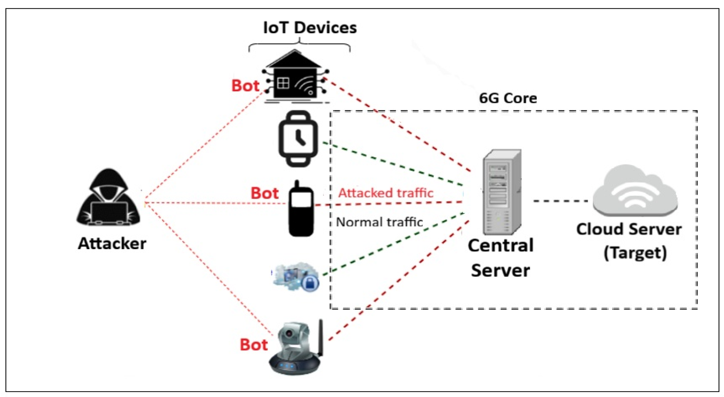
Figure 1 illustrates the distributed attack model in 6G-IoT networks. First, the attackers control a set of IoT devices distributed across various locations, known as botnets, to attack target servers. To detect attacks in 6G-IoT networks with low communication latency, we propose an intrusion detection system (IDS)-based collaborative Federated Learning (FL) (IDS-CFL). In addition, to improve accuracy, a Deep Convolutional Generative Adversarial Network (DCGAN) model is used to train the data. The following sections describe the details.

3.1. Intrusion Detection System Based Collaborative Federated Learning

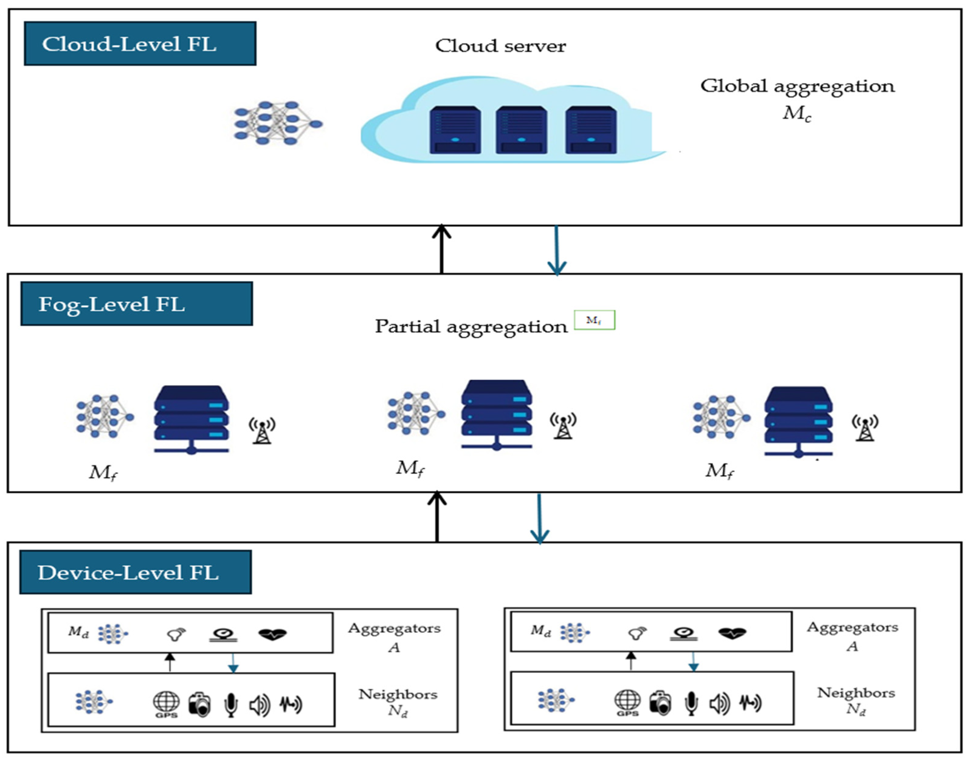
As shown in Figure 2, the proposed IDS-based collaborative FL (IDS-CFL) architecture comprises device, fog, and cloud levels. The device level consists of IoT devices and actuators. The fog level consists of fog servers with high computational capabilities to minimize computation delays; it is collected with Base Stations (BSs). The data for each device $u$ with size $\left|X_u\right|$ is represented with $X_u = \{({x^u}_1,{y^u}_1), \dots ,({x^u}_{\left|X_u\right|},{y^u}_{\left|X_u\right|})\}$, where $x$ is the input data and $y$ is the label for $x$. Each device $u$ trains its local model $M_u$ with its data. At the device level, devices can share data with neighbors to enable faster detection. Devices communicate via M2M to share data. To avoid bandwidth consumption and protect privacy, FL does not allow sharing raw data. It is adapted to train the global model $M$. To address the availability of fog/cloud infrastructure, the system optimally selects a suitable data-sharing mechanism by enabling dynamic collaboration among the learning levels the device participates in. The details are given below.

3.1.1. Cloud-Level FL

FL at the cloud level aims to train the global model $M_c$ using data from the IoT devices. First, the cloud broadcasts the initial parameter $w_0$ to all $U$ devices participating in the learning process. The learning process contains the local model parameter $w_c$ for $M_c$ that aims to minimize the global loss function $L_c\left(w_c\right)$ as

$$\mathit{min}{L}_c\left(w_c\right)={\displaystyle \frac{1}{U_c}}{\displaystyle \sum _{u=1}^{U_c}}{\displaystyle \frac{1}{P_u{X}_u}}{\displaystyle \sum _{j=1}^{P_u{X}_u}}{\displaystyle \frac{1}{P_u{X}_u}}l\left(w_d, x_{\mathit{uj}},y_{\mathit{uj}}\right)$$

(1)

where $P_u$ is the local batch for the device $u$ participating in cloud learning. $l\left(w, x_{\mathit{uj}}, y_{\mathit{uj}}\right)$ is the loss value for data sample $j$ for the device $u$. Each device minimizes the loss function on its own data using gradient descent, with a lower bound of 0 and an upper bound of 1. The devices participating in cloud learning transmit their local parameters to the BSs at the fog level for partial aggregation. Fog servers perform partial aggregation with the FedAvg algorithm. The partial aggregation of the model at the fog level $M_f$ is calculated as

$$M_f={\displaystyle \frac{1}{U_f}}{\displaystyle \sum _{u=1}^{U_c}}\left(P_u\left|X_u\right|\right){·w}_u$$

(2)

where $U_c$ is the number of devices under the coverage of BSs that participate in cloud learning. $P_u\left|X_u\right|$ is the data size of device $u$ included in the partial aggregation process. The $w_u$ is the model weight parameter of device $u$. The BSs then transmit the partial aggregations to the cloud for global aggregation. The global model $M_c$ is aggregated as

$$M_c={\displaystyle \frac{1}{M}}{\displaystyle \sum _{i=1}^M}{M}_f$$

(3)

After the global model update, the cloud sends the updated parameters to the BSs, which then forward them to the devices included in the cloud learning. For fog-level learning, we can use the equations above. The BSs transmit $M_f$ model parameters to the devices under their coverage.

3.1.2. Device-Level FL

At the device level, the aggregator $A$ and neighboring devices $N_d$ can perform global model aggregation. Learning process contains the local model parameter $w_d$ for $M_d$ that aims to minimize the global loss function $L_c\left(w_c\right)$ as

$$\mathit{min}{L}_d\left(w_d\right)={\displaystyle \frac{1}{U_d}}{\displaystyle {\sum }_{u=1}^{U_d}}{\displaystyle \frac{1}{P_u{X}_u}}{\displaystyle {\sum }_{j=1}^{P_u{X}_u}}{\displaystyle \frac{1}{P_u{X}_u}}l\left(w_d, x_{\mathit{uj}},y_{\mathit{uj}}\right)$$

(4)

As in cloud-level FL, each device minimizes the loss function on its own data using gradient descent. Afterward, the randomly selected aggregator receives the local parameters $w_d$ from its neighboring devices to perform aggregation process. The aggregator calculates the weighted average of the neighboring devices’ parameters. All aggregators receive the parameters from their neighboring devices in parallel. The aggregation process for $M_d$ model at the device level is calculated as

$$M_d={\displaystyle \frac{1}{U_d}}{\displaystyle \sum _{u=1}^{U_d}}\left(P_u\left|X_u\right|\right){·w}_u·{\gamma }_u$$

(5)

where ${\gamma }_u$ is the weighted average coefficient. For privacy, devices do not share raw data. Each device near the aggregator is included in the device-level FL. For simplicity, we assume all neighboring devices are included in the device-level FL.

3.2. Problem Formulation

As mentioned above, the current IDSs have multiple challenges, including communication latency and learning performance. The first optimization problem considers the communication latency, which is high in FL because of the large volume of data and parameters transmissions. By minimizing data transmissions, the detection time decreases. At each FL iteration, a device’s detection time is the time needed to receive the updated parameters and train the model. The first objective function is to minimize detection time $T$ subject to a maximum CPU frequency $L$ constraint. It can be modeled as

$$z=\mathit{min} \left(T\right)$$

(6)

subject to

$$L^{\mathit{min}} \le L_{u }\le L^{\mathit{max}}$$

This time is calculated based on the device’s learning level. The following represent the calculations for the devices included in the learning.

The second optimization problem considers learning performance, which must be optimized to improve detection accuracy. The second objective function maximizes detection accuracy by minimizing loss function $L\left(w\right)$ at each learning level, with a massively distributed data constraint where the global data $X$ is stored across a large number of devices. It can be modeled as

$$J\left(w\right)={ \mathit{min}}_{X_u} \left(L\right(w\left)\right)$$

(7)

subject to

$${\displaystyle {\sum }_{u=1}^U}{X}_u=X$$

3.2.1. Detection Time in CFL

To solve the first optimization problem, we minimize the detection time at each learning level, as explained below.

• Cloud level:

• Local training: The local training time at device $u$ depends on the device’s data size. The local training time is calculated as

  $$T_{\mathit{loc}\_u}={\displaystyle \frac{P_u\left|X_u\right|}{L_u^k}}{L}^k$$

  (8)

  where $L^k$ is the number of CPU cycles required to train one data sample, and $L_u^k$ is the device CPU frequency.
• Model aggregation: The partial aggregation time at BS $i$ consists of the time required to transmit the parameters from the devices that participate in the cloud level under BS’s coverage area. The partial aggregation time at BS $i$ is calculated as

  $$T_{\mathit{agr}}^i={\displaystyle \frac{\left|w_u\right|}{R_{u,i}}}+{\displaystyle \frac{|R_i||w_g|}{L_i^k}}{L}_w^k$$

  (9)

  where $\left|w_g\right|$ is the size of global model, it is the same size as local model $\left|w_u\right|$, $L_w^k$ is the number of CPU cycles required to aggregate one unit of data, and $L_i^k$ is the CPU frequency of BS $i$. The aggregation time at the cloud server is calculated as

  $$T_{\mathit{agr} }=\left(T_{\mathit{agr}}^i+{\displaystyle \frac{\left|w_g\right|}{R_{c,i}}}\right)+{\displaystyle \frac{\left|w_g\right|}{L_c^k}}{L}_w^k$$

  (10)

  where $R_{c,i}$ is the bandwidth communication between BS $i$ and cloud server, and $L_c^k$ is the CPU cycle at the cloud server. The aggregation time is affected by the large amount and diversity of data, which makes the system more scalable.
• Parameter transmission: The required time depends on the parameters download at device $u$ under BS $i$ coverage and is based on the parameter size. The required time for the transmission between the cloud server and BS $i$, and between BS $i$ and device $u$, is calculated as

  $$T_{\mathit{tsm}}\left(u\right)={\mathit{log}}_2{\displaystyle \frac{\left|w_u\right|}{R_{c,i}}}+{\displaystyle \frac{\left|w_u\right|}{R_{u,i}}}$$

  (11)

In the aggregation phase, the detection time in a single iteration for device $u$ that takes part in the cloud level is calculated as

$$T\left(u\right)={\mathit{max}}_u\left\{T_{\mathit{loc}\_u}\right\}+{\mathit{max}}_u\left\{{\mathit{log}}_2{T}_{\mathit{tsm}}\left(u\right)\right\}$$

(12)

2.

Device level: At the device level, the model parameters can be shared across neighborhood devices, with one device selected as the aggregator. The detection time for the aggregator $u$ in one iteration is calculated as

$$T\left(u\right)={\mathit{max}}_{n\in u}\left\{T_{\mathit{loc}\_n}\right\}+{\displaystyle \frac{T_{\mathit{agr}}^u}{L_u^k}}$$

(13)

It includes the time required for local training at device $u$ and neighborhood devices, as well as the time to transmit the model parameters from neighborhood devices. The aggregation time is represented as

$$T_{\mathit{agr}\_u}={ \mathit{max}}_{n\in N_u}{\displaystyle \frac{\left|w_n\right|}{R_{n,u}}}+{\displaystyle \frac{N_u\left|w_g\right|}{L_u^k}}{L}_w^k$$

(14)

where $R_{n,u}$ is the transmission rate of the neighborhood device $n$ to connect to device $u$. When the neighborhood device $n$ participates at the device level but is not selected as an aggregator, it downloads the parameters after the aggregation process. The detection time for the neighborhood device $n$ is calculated as

$$T\left(n\right)={ \mathit{max}}_{u\in N_u}\left\{T_{\mathit{loc}\_\stackrel{\mathrm{-}}{u}}\right\}+{\displaystyle \frac{\left|w_g\right|}{R_{n,u}}}+{\displaystyle \frac{T_{\mathit{agr}}^u}{K_n^k}}$$

(15)

3.

Device selection algorithm: Collaboration across multiple levels can improve detection accuracy but may increase service delivery delays or cause service unavailability in locations far from cloud or fog servers. Therefore, device-level collaboration can minimize time consumption and enable faster detection. Moreover, selecting a device far from the aggregator takes time and adds transmission latency. Therefore, a Gray Wolf Optimizer (GWO) optimization algorithm is used for device selection at the device level. The GWO is a metaheuristic algorithm that mimics the social hierarchy and hunting behaviors of the grey wolves to catch prey in nature. It is used to solve various problems, including global optimization problems because it has fewer parameters, simple principles, and easy implementation [27]. In GWO, five solutions represent the devices in the search space, where alpha (α) is the best solution, beta (β) is the second-best solution, delta (δ) is the third-best solution, and omega (ω) is the rest of the solutions. The wolf represents aggregator A, which is selected randomly, while prey represents neighboring devices $A_n$. The best three solutions (α, β, δ) are used to guide the other solutions (ω) to improve the search space. The selection steps are described as follows.

• Encircling: Aggregator $A$ starts by forming a circle around the neighboring devices $A_n$ when hunting. It is represented mathematically as

  $$E=\left|C \times { A}_n \left(t\right)-A\left(t\right)\right|$$

  (16)

  $$A\left(t+1\right)=A_n\left(t\right)-S \times P$$

  (17)

  where $t$ is the iteration number, $A_n$ is the neighboring device position, $A$ is the aggregator position, $P$ is used to specify a new position of the aggregator, and $S$ and $C$ are coefficient vectors that are calculated as

  $$S=2a \times r_1-a$$

  (18)

  $$C=2r_2$$

  (19)

  where $r_1$ and $r_2$ are random vectors in [0, 1], $a$ is a vector decreased linearly from 2 to 0 over the iterations, and is calculated as

  $$a={\displaystyle \frac{2-t \times 2}{{\mathit{max}}_{\mathit{itr}}}}$$

  (20)
• Hunting: In this step, the best three solutions (α, β, δ) are obtained. As for the other solutions (ω), they need to update their position by moving towards the average of the three best and known positions, since they have better knowledge about the optimal location of the neighboring device. This step is represented mathematically as

  $$A_i\left(t+1\right)=A_i\left(t\right)-a_i \times P_i$$

  (21)

  $$V_i=\left|C_i \times { A}_i\left(t\right)-A\left(t\right)\right|$$

  (22)

Let $V_i$ is the positive weight associated with aggregator $i \in \{\alpha ,\beta ,\delta \}$ such that $\sum _i{V}_i = 1$. The aggregators’ positions $\alpha$, $\beta$, and $\delta$ are a good estimation of the average position of the optimal solution at iteration $t$, it is represented as

$$A\left(t+1\right)=\sum _{i\in \{\alpha ,\beta ,\delta \}}{V}_i \times A_i(t+1)$$

(23)

• Attacking: The aggregators finish the hunt by attacking the neighboring device until they stop moving. To model the attacking process, Equation (20) is used, as the parameter $a$ balance exploration and exploitation; a decrease linearly from 2 to 0 over iterations. Consequently, parameter $S$ takes a random value in the range [$-2a, 2a$] given by Equation (18). When $S > 1$ or $S < -1$, aggregators take a random position; when $-1 \le S \le 1$, they are forced to move toward the neighboring device.

Algorithms 1 and 2 describe the CFL procedure and device selection.

Algorithm 1: Collaborative FL

Input: Device $u \in U$, initial global parameter $w_0$, local patch $P_u$ of device $u$, data size $X_u$ of device $u$, input data $X$ Output: Updated global model //Initialization Cloud server initialize $w_0$ for each iteration $t = 0, 1, 2, \dots , T$ do      //Cloud-Level FL      Select a random set $U$ of $u$ devices      Broadcast $w_0$ to all $U$ devices participating at the cloud level      Receive partial aggregation $M_f$ from the fog level and perform global aggregation $M_c$ using Equation (3)      Updated $w_c$ and $w_u$ parameters      Send updated $w_u$ to BSs participating in the learning      //Fog-Level FL      Each device $u$ sends its local parameters $w_u$ to BSs      Fog server performs partial aggregation $M_f$ using Equation (2)      Send $M_f$ to cloud      Receive updated $w_u$ from cloud      Update parameters $w_f$ and $w_u$      Send $w_u$ to devices $U$ participating in the learning      //Device-Level FL      Select aggregator $A$ randomly      Aggregator $A$ receives $w_d$ from neighboring devices $N_d$      Aggregator $A$ performs aggregation $M_d$ using Equation (5)      Update parameters $w_d$ and $w_u$ end for

Algorithm 2: Device selection using GWO

Input: Population size of aggregator devices $A$ Output: Optimally aggregator position $A_{\alpha }$ from Neighboring devices $N_d$ Initialize the aggregator population randomly $A_n$ Initialize $a$, $S$, and $C$ Calculate the fitness of each search agent $A_{\alpha }$ is the best solution $A_{\beta }$ is the second-best solution $A_{\delta }$ is the third-best solution while $t <{ \mathit{max}}_{\mathit{itr}}$ do      for each aggregator $A_n$ do            Initialize $r_1$ and $r_2$ randomly            Update current position using Equation (23)      end for Update $a$, $S$, and $C$ Calculate fitness of each aggregator $A_n$ Update $A_{\alpha }$, $A_{\beta }$, and $A_{\delta }$ $t = t + 1$ end while return $A_{\alpha }$ (set of devices participating in device-level FL)

3.2.2. Deep Convolutional Generative Adversarial Network

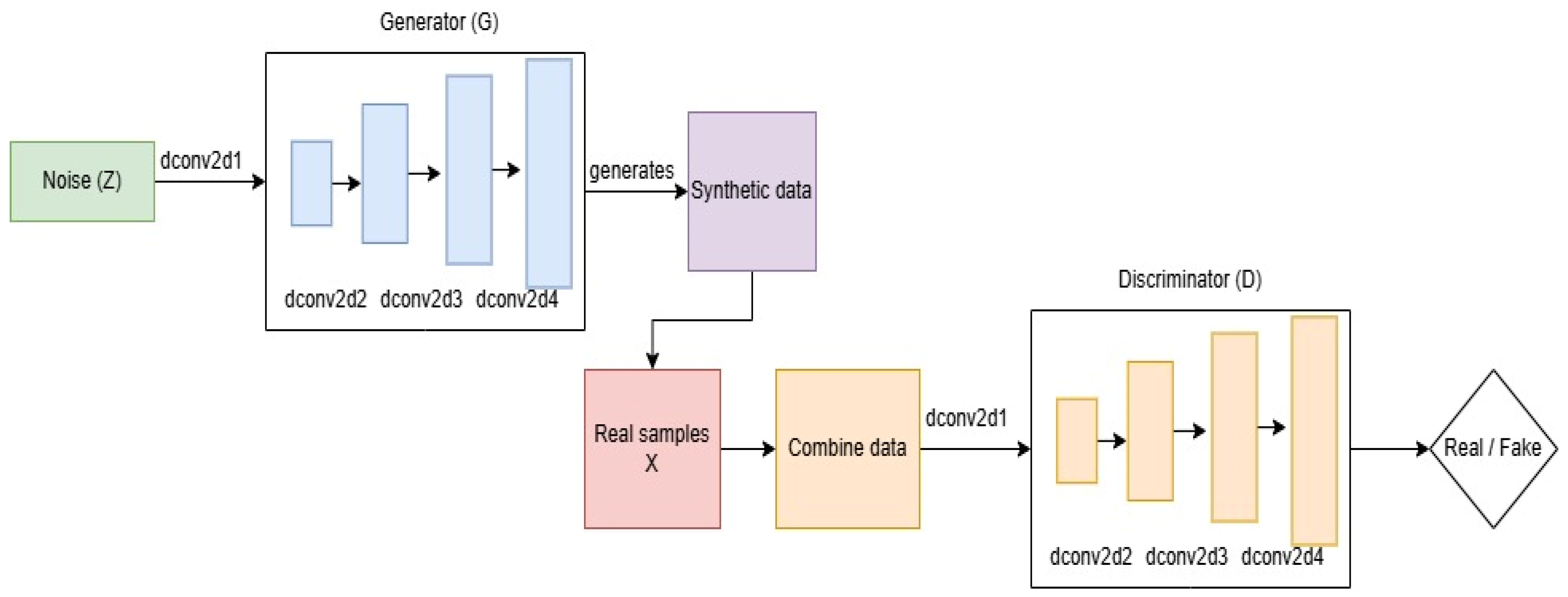
To solve the second objective function and achieve high accuracy and fast processing, we use Deep Convolutional Generative Adversarial Network (DCGAN) model to train data at each level. It enables fast processing by replacing heavy fully connected layers with efficient convolutional layers. It can learn complex patterns and feature representations from large datasets. DCGAN improves detection performance by generating synthetic attack samples to train stronger detection models. The architecture of DCGAN is shown in Figure 3, it consists of a generator $\mathit{GE}\left(z\right)$ and a discriminator $\mathit{DE}\left(x\right)$.

The generator takes a random noise vector $z$ and upsamples it by using fractionally strided convolutions to output 2D synthetic data. The discriminator distinguishes between generated and real data. The DCGAN is mathematically described as

$${\mathit{min}}_{\mathit{GE}} {\mathit{max}}_{\mathit{DE}}L\left(\mathit{GE}\left(z\right),\mathit{DE}\left(x\right)\right)$$

(24)

The loss function $L$ at each level is represented as

$$L=E_{x~X_{\mathit{train}}}[\mathit{log}\mathit{DE}\left(X\right)\left)\right]+E_{z~X_z}[\mathit{log}(1-D\left(\mathit{GE}\left(X\right)\right)\left)\right]$$

(25)

where $E$ is the expectation, $X_{\mathit{train}}$ is the training data distribution variable, $x$ is the input vector, $X_z$ is the noise distribution variable, and $z$ is a noise vector.

In the generator, the data $z$ is sampled from the random $X_z$ as the generator input. It converts the 100-dimentional noise signal into $(4 \times 4 \times 1024)$ 3D tensor using a fully connected layer; four convolution operation are applied sequentially, each with a different number of channels. Each operation uses a $(4 \times 4)$ convolution kernel and a stride of 2, converting the feature map array into an output map array $(64 \times 64 \times 3)$. Batch normalization is introduced after each transpose convolution to improve training speed, stability, and performance. After that, the ReLU function introduces nonlinearity through setting negative values to 0 and keeping positive values unchanged; this helps the network learn patterns. The synthetic data $X_z^{\prime } = \mathit{GE}(X_z)$ is generated, the synthetic generation process can be explained as

$$x_{z }^l=v^l{\left(w_{\mathit{ge}}^l\right)}^M \times x_z^{l-1}+b_{\mathit{ge}}^l$$

(26)

where $x_z^l$ is the output data $z$ at layer lth. $w_{\mathit{ge}}^l$ and $b_{\mathit{ge}}^l$ are the weight and bias parameters of $\mathit{lth}$ convolutional layer. $v^l$ is the ReLU activation function for all layers except the output layer, which uses Tanh activation.

Now, the synthetic data $X_z^{\prime }$ is combined with the input data $X_{\mathit{train}}$ to generate combined data $X_{\mathit{de}}$ that used to train the discriminator. It is configured with three $(2 \times 2)$ convolution kernel with a stride of 2.

The discriminator has four convolutional layers and takes a $(64 \times 64 \times 3)$ input. The four convolutional layers use LeakyReLU except the output layer, which uses Sigmoid. Each operation uses a $(4 \times 4)$ convolution kernel and a stride of 2, converting the feature map array into an output map array $(1 \times 1)$. After training, the discriminator generates the discriminator data $Y_{\mathit{de}}$ where $Y_{\mathit{de}} = \mathit{DE}(X_{\mathit{de}})$. Finally, the data from the discriminator needs to be preprocessed, which can be defined as

$$Y_{\mathit{de}}=\left\{\begin{array}{c}{y}_{l1}=0, y_{l2}=1 if y_{l1} < y_{l2}\\ y_{l1}=1, y_{l2}=0 if y_{l1} \ge y_{l2}\end{array}\right.$$

(27)

where $y_{l1}$ and $y_{l2}$ are the discriminator outputs of the $\mathrm{lth}$ data of the discriminator. The output $Y_{\mathit{de}}$ is contain $Y_z$ and $Y_{\mathit{train}}$, where $Y_z$ is the discriminant output of synthetic data $X_z^{\prime }$ and $Y_{\mathit{train}}$ is the discriminant output of data $X_{\mathit{train}}$. Now, the discriminator performance of $Y_z$ and $Y_{\mathit{train}}$ are calculated using accuracy $\mathrm{ACU}$ function as

$$\mathit{ACU}={\displaystyle \frac{\mathit{TP}+\mathit{TN}}{\mathit{TP}+\mathit{TN}+\mathit{FP}+\mathit{FN}}}$$

(28)

The second objective function is improving accuracy by obtaining optimal discriminator performance; we can redefine the loss function as

$$L\left(\mathit{GE},\mathit{DE}\right)=E_{x~X_{\mathit{train}}}[\mathit{log}\left(\mathit{ACU}\right(\mathit{DE}\left(X\right)\left)\right)]+E_{z~X_z}[\mathit{log}(1-\mathit{ACU}(\mathit{DE}\left(\mathit{GE}\left(X\right)\right)\left)\right)]$$

(29)

The optimal discriminator ${\mathit{DE}}_{\mathit{ge}}^{*}$ is obtained as

$${\mathit{DE}}_{\mathit{ge}}^{*}=\mathit{arg}{\mathit{max}}_{\mathit{de}}{L}_{\mathit{DCGAN}}({\mathit{GE}}_{\mathit{de}}^{*}, \mathit{DE})$$

(30)

where ${\mathit{GE}}_{\mathit{de}}^{*}$ is the optimal generator performance which is obtained as

$${\mathit{GE}}_{\mathit{de}}^{*}=\mathit{arg}{\mathit{min}}_{\mathit{ge}}{L}_{\mathit{DCGAN}}(\mathit{GE}, {\mathit{DE}}_{\mathit{ge}}^{*})$$

(31)

Algorithm 3 illustrates the overall DCGAN training process.

Algorithm 3: DCGAN algorithm

Input: Number of epochs ($n\_\mathit{epochs}$), batch size ($n\_\mathit{batch}$), initial generator weight ${\theta }_{\mathit{ge}}$, initial discriminator weight ${\mathrm{\theta }}_{\mathrm{de}}$, generator ($\mathit{GE}$), discriminator ($\mathit{DE}$), training data distribution ($X_{\mathit{train}}$), noise distribution $X_z$, input vector ($x$), noise vector ($z$) Output: Optimally trained ${\mathit{DE}}_{\mathit{ge}}^{*}$ and ${\mathit{GE}}_{\mathit{de}}^{*}$ //Initialization Initialize ${\theta }_{\mathit{ge}}$ and ${\theta }_{\mathit{de}}$                             for each epoch from 1 to $n\_\mathit{epochs}$ do                                 Shuffle training data and create minibatches                                     for each batch from 1 to $n\_\mathit{batch}$ do                                          //Generator training                                                  Sample minibatch of $m$ noise samples $\left\{z_1,z_2,\dots ,z_m\right\}$ from $X_z$                                                    Sample minibatch of $m$ real data samples $\left\{x_1,x_2,\dots ,x_m\right\}$ from $X_{\mathit{train}}$                                                    Generate synthetic data $\{{\mathit{GE}}_{(z_{1)}},{\mathit{GE}}_{(z_{2)}},\dots ,{\mathit{GE}}_{(z_{m)}}\}$ using Equation (26)                                                    Combine synthetic data $X_z^{\prime }$ with $X_{\mathit{train}}$ to generate combined data $X_{\mathit{de}}$                                                    Update $\mathit{DE}$ using Adam: ${\nabla }_{{\theta }_d}{\displaystyle \frac{1}{m}}{\displaystyle {\sum }_{i=1}^m}[\mathit{log}\mathit{DE}\left(x_i\right)+\mathit{log}(1-\mathit{DE}\left(\mathit{GE}\left(z_i\right)\right)\left)\right]$                                          //Discriminator training                                                    Evaluate discriminator output $Y_{\mathit{de}}$ using Equation (29)                                                    Sample minibatch of $m$ noise samples $\left\{z_1,z_2,\dots ,z_m\right\}$ from $X_z$                                                    Generate fake data samples $\{{\mathit{GE}}_{(z_{1)}},{\mathit{GE}}_{(z_{2)}},\dots ,{\mathit{GE}}_{(z_{m)}}\}$                                                    Update $\mathit{GE}$ using Adam:                                                         ${\nabla }_{{\theta }_g}{\displaystyle \frac{1}{m}}{\displaystyle \sum _{i=1}^m}\mathit{log}(1-\mathit{DE}\left(\mathit{GE}\left(z_i\right)\right))$                                          end for                                 Calculate ${\mathit{DE}}_{\mathit{ge}}^{*}$ using Equation (30)                                 Calculate ${\mathit{GE}}_{\mathit{de}}^{*}$ using Equation (31)                                 Save ${\mathit{DE}}_{\mathit{ge}}^{*}$ and ${\mathit{GE}}_{\mathit{de}}^{*}$                             end for

4. Data Preparation

This section describes the dataset used for evaluation and the preprocessing steps used to prepare the training and testing sets.

4.1. Data Description

This paper uses a recent, comprehensive, realistic cybersecurity dataset for IoT and IIoT applications, called Edge-IIoTest [28]. It supports intrusion detection systems in both centralized and FL modes. The dataset is generated using a purpose-built IoT/IIoT testbed with a large representative set of devices, sensors, protocols, and cloud/edge configurations. Multiple devices (over 10 types) generate the IoT data. It includes five types of threats: DoS/DDoS attacks, Information gathering, Man in Middel attacks, Injection attacks and Malware attacks. The dataset contains 61 features from different sources, with 1176 features found to be highly correlated.

4.2. Data Preprocessing

IoT traffic includes normal traffic and various types of attacks. We apply the following preprocessing techniques to prepare the dataset for training.

• Feature mapping: The features in IoT data do not consist only of numeric values. Therefore, a mapping technique is required to convert categorical values to numeric values. A common method is One-Hot Encoding (OHE), which converts each distinct value into a binary value.
• Data normalization: Normalization is a scaling method that converts all data features onto a common scale. We removed outliers, such as null values and non-numeric entries in numerical attributes. For a fair comparison, we have normalized the dataset using Min-Max scaling. This popular method facilitates arithmetic processing by linearly mapping each feature’s range to 0–1. It can be calculated as

$$X_{\mathit{scale}}={\displaystyle \frac{X-X_{\mathit{min}}}{X_{\mathit{max} }- X_{\mathit{min}}}}$$

(32)

3.

Feature Selection: It improves predictive quality by selecting relevant features. Feature selection is the process of selecting a subset of features important for solving the detection problem and discarding unneeded features. In this paper, we use a mutual information (MI) technique for feature selection, with selection criteria based on feature dependencies: features with high mutual information are considered the best features. The input–output variables from the training set can be represented as $X$ and $Y$ where $R=\left\{X, Y\right\}$. To compute MI, follow these steps.

Step 1: Measure the dependencies between input and output variables $\mathit{MI} = \{X_i, Y\}$ as

$$\mathit{MI}(X,Y)=\sum _{x\in X}\sum _{y\in Y}\mathit{PR}(x, y)\mathit{log}{\displaystyle \frac{\mathit{PR}(x, y)}{\mathit{PR}\left(x\right)\times \mathit{PR}\left(y\right)}}$$

(33)

where $\mathit{PR}\left(x\right)$ and $\mathit{PR}\left(y\right)$ are the marginal distributions, and $\mathit{PR}(x, y)$ is the joint probability of $X$ and $Y$.

Step 2: Remove any values less than other values and maintain the remaining in a vector $V$. Now, the input and output variables can be represented as $R_{\mathit{new}}$, sorted in descending order based on the value of $V$.

Step 3: Define the number of selected features represented as $F$ and select the first input–output $F$ variable from $R_{\mathit{new}}$ as a selected features to form $R_F$.

Step 4: Select the variable with the highest $\mathrm{MI}$ as a first variable in $R$. Now, select $\mathit{jth}$ variables $(1 \le j \le F)$ from $R_F$ and compute $\mathit{MI}(S,{ X}_j)$ values. If $\mathit{MI}(S,{ X}_j) \le \alpha$, $R \cup X_j$, where $\alpha$ is the threshold value. Otherwise, ${ X}_j$ will have less dependency and need to be deleted.

4.

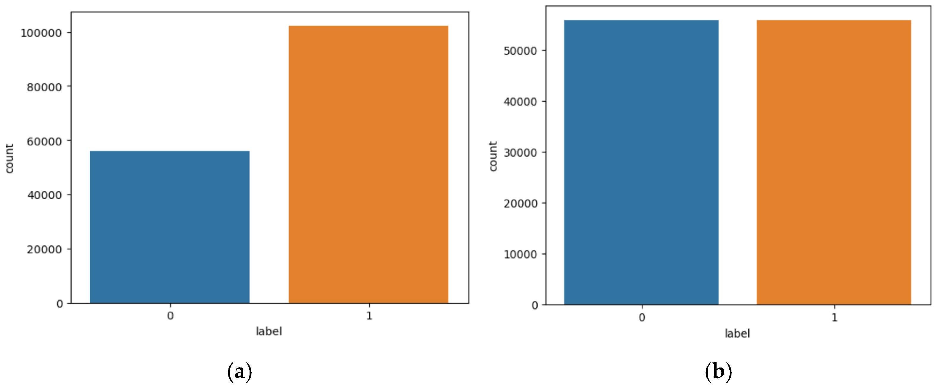
Class Balancing: To prevent bias toward the majority “Normal” class, the script identifies the minority class size and samples from it. The Synthetic Minority Over-sampling Technique (SMOTE) [29] is applied to handle the imbalanced dataset. It is based on the K-Nearest Neighbors (KNN) model, which takes samples and considers their nearest neighbors in the feature map. If $\left(x_1, x_2\right)$ is a sample of a minority class and if its neighbor is selected as $(x_1^{*},x_2^{*})$, then the data point is synthesized as

$$(X_1, X_2)= (x_1, x_2)+\mathit{random}(0, 1) \times ∆$$

(34)

where $∆ = \left\{\right(x_1^{*},x_1), {(x}_2^{*},x_2\left)\right\}$, $\mathit{random}(0, 1)$ is a random value between 0 and 1. Figure 4 shows the data before and after data balancing.

5. Experimental Results

This section describes the experimental setup and compares the proposed IDS-CFL with distributed and centralized methods across different experiments.

5.1. Experiment Setup

For evaluation, the experiment is conducted in a 6G-IoT simulation environment combining cloud, fog, and device levels. The NS-3 simulator was used to build a 6G network environment with 50 distributed devices collaborating in the detection process. The simulation environment was configured with network parameters that align with 6G specifications. The CFL channel model is based on uplink massive MIMO technology to achieve the high throughput and efficiency needed for 6G-IoT networks. The channel model consists of 5 BSs equipped with fog servers located between the cloud and device level, with a CPU frequency of 2.5 GHz. All fog nodes have identical computing capabilities. The transmission bandwidth is 100 MHz, and the coverage radius is 250 m. The devices’ CPUs are randomly selected between 1.5 to 2.4 GHz based on device capabilities. We use TensorFlow and Keras DL libraries to implement the DCGAN model. We adopt an 80:20 split, allocating 80% of the data for training and 20% for testing. We found that a learning rate of 0.01 is appropriate for our system. The parameter settings utilized in the implementation are detailed in

Table 2. Parameters setting.

Parameter	Value
No. of devices	50
No. of BSs	5
Data rate	10 Mbps
Fog CPU frequency	2.5 GHz
Device CPU frequency	from 1.5 to 2.4
Transmission bandwidth	100 MHz
Learning rate	0.01
Batch size	128
Epochs	10
Optimizer	Adam

.

5.2. Performance Metrics

We applied different performance metrics to evaluate the effectiveness of the proposed system, including detection time, accuracy, recall, f-measure (F1), and Area Under Curve (AUC).

5.3. Performance Analysis

The performance of the proposed IDS-CFL system is evaluated and compared with different methods, including

• No FL: In this model, centralized learning is performed where each device sends its data to the cloud for model training.
• Fog-level FL: In this model, the traditional FedAvg method is performed at the fog level. The devices send their data to the fog level for model training. After training, the fog servers send the local parameters to the cloud for global model aggregation. After that, the cloud sends the updated parameters to the fog level to update the model.
• Device-level FL: In this model, at each FL iteration, the devices train the model using their data and, instead of sending local model parameters to the cloud or fog, share their parameters. The selected aggregator receives the parameters from neighboring devices and aggregates the model. After that, the aggregator sends the results back to the neighboring devices for attack detection. The aggregator device is selected randomly, and neighboring devices are selected based on the k-means clustering as in [30].

5.4. Results

The experimental performance of the proposed CFL is compared with the other methods through different experiments to evaluate its effectiveness. These experiments are explained in the following.

5.4.1. Experiment 1: Effect of Collaboration in CFL

In this experiment, we examined the involvement of devices and collaboration across different learning levels in FL using two scenarios (S1 and S2), as shown in

Table 3. Devices’ involvement during learning levels.

Method	Total Involved Device Ratio in FL	Device-Level Collaboration Ratio	Fog-Level Collaboration Ratio
No FL	0	0	0
Fog-level FL	S1: 70%, S2: 90%	0	100%
Device-level FL	S1: 30%, S2: 40%	100%	0
CFL	90%	25%	75%

.

• S1: In S1, there are no devices in No FL involved in learning. In fog-level FL, a high portion of devices is involved in FL (70%), whereas device-level FL involves the lowest portion (30%). This is because 30% of devices have neighbors. CFL has the highest device involvements, at 90% in FL. BSs can cover up to 80% of devices, and devices without BS access can collaborate in FL through their neighboring devices, if available. Also, if a device has no neighbors, it can participate in FL at the fog level if fog infrastructure is available. For our CFL, 10% of devices are not covered by any BS or neighbors.

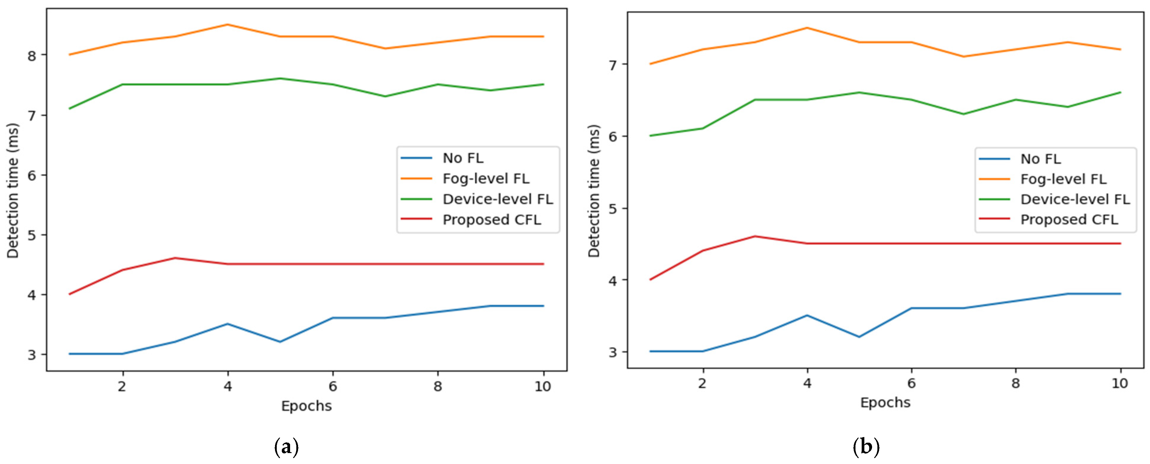
Figure 5a compares the proposed CFL with the other methods with S1 in terms of detection time. No FL achieves the lowest detection time with 3.8 ms, as it performs only local training. Device-level FL achieves 7.5 ms detection time because it takes time to transmit parameters. Training takes around 4.5 ms, and aggregation takes 3 ms. Fog-level FL has the highest detection time, around 8.3 ms, due to the overhead transmitting parameters to the BSs. The proposed CFL outperforms the device level and fog level with 4.5 ms. This is because the CFL enables collaboration between the device level and fog level, which minimizes detection time. In addition, using GWO algorithm helps to reduce detection time and increase accuracy compared with k-mean clustering selection method.

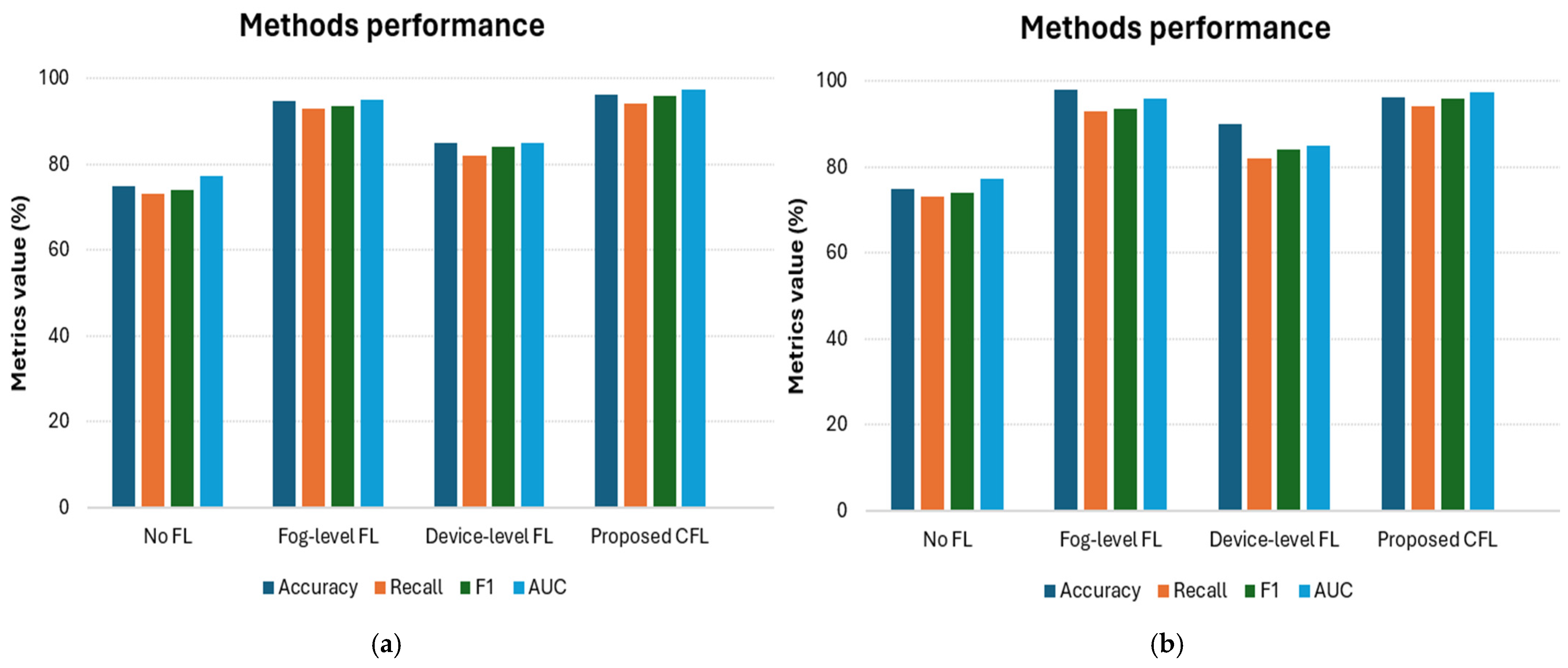
As shown in Figure 6a, our proposed CFL model achieves the highest values: 96.20% accuracy, 94.10% recall, 95.90% f-measure, and 97.05% AUC. No FL achieves the lowest performance because it does not share data. Fog-level FL outperformed the device-level FL with 94.80% accuracy, 92.99% recall, 93.52 f-measure, and 95.03% AUC. This is because fog-level FL shares parameters across 70% of devices, compared with 40% in device-level FL. The proposed CFL learns to optimize accumulated detection accuracy by exploiting fog-level FL.

2.

S2: In S2, the fog servers’ capabilities are available for 90% of devices, whereas 40% of devices have a neighboring. As shown in Figure 5b, there is no significant difference in detection time compared with S1. The time decreases by around 6.6 ms in device-level FL and 7.2 ms in fog-level FL. As shown in Figure 6b, the accuracy and the other metrices are increased in fog-level FL which scored 97.99%. In device-level FL, performance is better than in S1, with 90.06% accuracy when 40% of devices have a neighborhood. Compared with fog-level FL, our CFL reduced communication because it shares parameters across 90%. On the other hand, it outperformed No FL and device-level FL.

Table 4. Methods comparative results.

Method/Metrics	Accuracy (%)	Recall (%)	F1 (%)	AUC (%)	DT (ms)
No FL	75.02	73.11	74.05	77.13	3.8
Fog-level FL	94.80	92.99	93.52	95.03	8.3
Device-level FL	85.09	82.12	84.19	85.03	7.5
Proposed CFL	96.20	94.10	95.90	97.05	4.5

summarized the comparison results.

5.4.2. Experiment 2: Comparing DCGAN with Other Models

In this experiment, we apply the proposed CFL to the GAN and CNN models to validate DCGAN’s performance. The traditional GAN is performed as in [31]. The CNN architecture comprises four convolutional layers; each pair of convolutional layers is followed by one max-pooling layer. Conv 1 and Conv 2 operated with (convolution filters = 16, filter size = 3, and output shape = 16 × 196 feature matrix), max-pooling 1 with pooling size = 2, Conv 3 and Conv 4 operated with (convolution filters = 32, filter size = 3, and output shape = 16 × 128 feature matrix), and max-pooling 2 with pooling size = 2. For fully connected layers, the model consists of three layers, each followed by a dropout layer. One padding is applied before each convolution operation, and ReLU is used as the activation function in the hidden layers. Sigmoid activates the last fully connected layer.

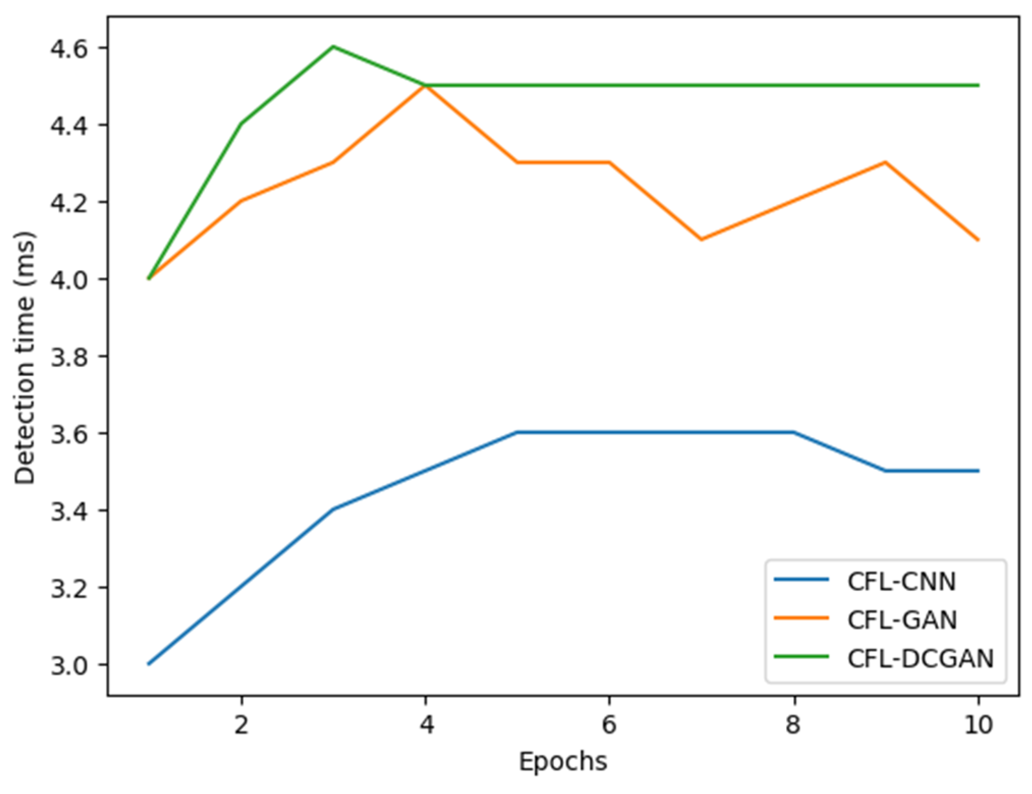
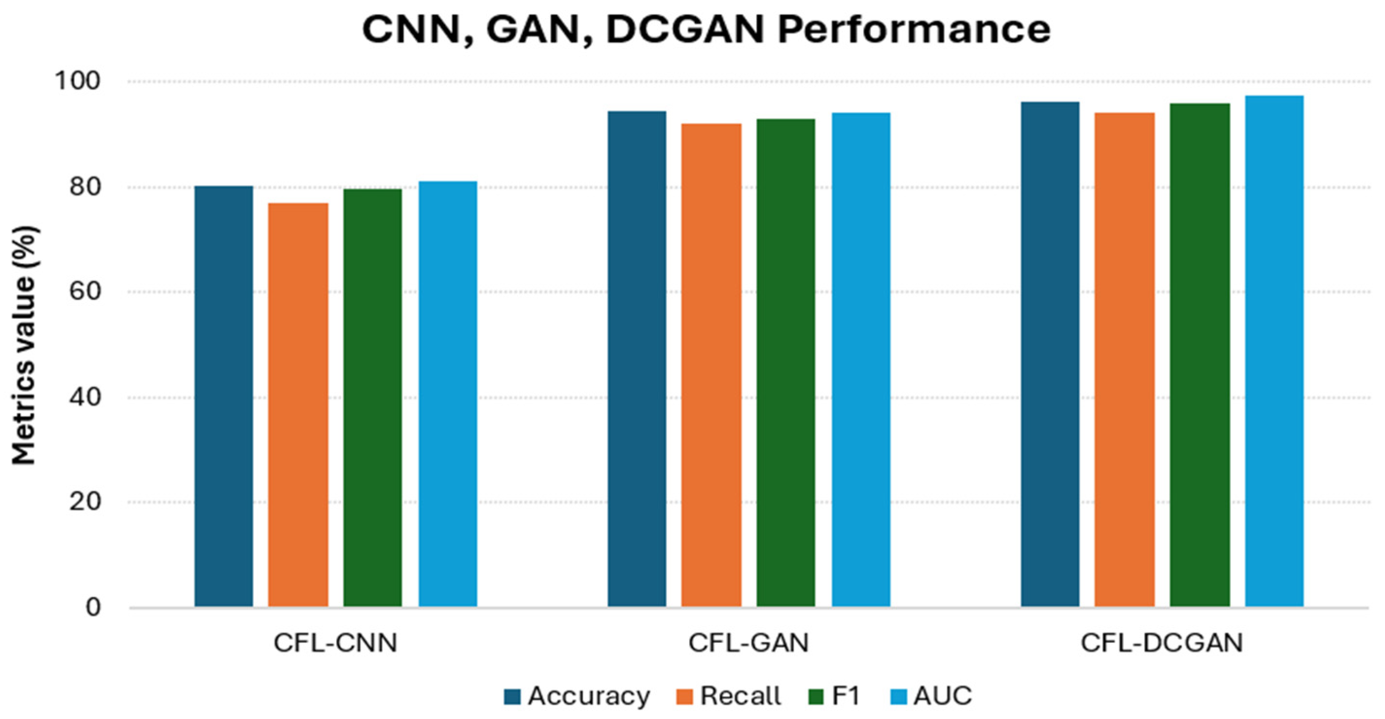
As shown in Figure 7, CNN outperformed DCGAN and GAN with 3.5 ms, with training time of about 2 ms and aggregation time of 1.5 ms. This is because CNN solves a simple mapping problem with a single network, whereas DCGAN and GAN involve training two adversarial networks simultaneously. Figure 8 shows that the CFL with DCGAN outperformed the GAN and CNN models in accuracy, recall, f-measure, and AUC. The GAN model had the highest values after DCGAN, with scored 94.32% accuracy, 92.16% recall, 92.98% f-measure, and 94% AUC. The CNN model performed the worst among the DCGAN and GAN models.

Table 5. Comparison results of different models in CFL.

Model/Metrics	Accuracy (%)	Recall (%)	F1 (%)	AUC (%)	DT (ms)
CNN	80.14	76.99	79.56	81.17	3.5
GAN	94.32	92.16	92.98	94	4.1
DCGAN	96.20	94.10	95.90	97.05	4.5

summarizes the comparison results of different models.

5.4.3. Experiment 3: Examine the Scalability with Increasing Number of Devices

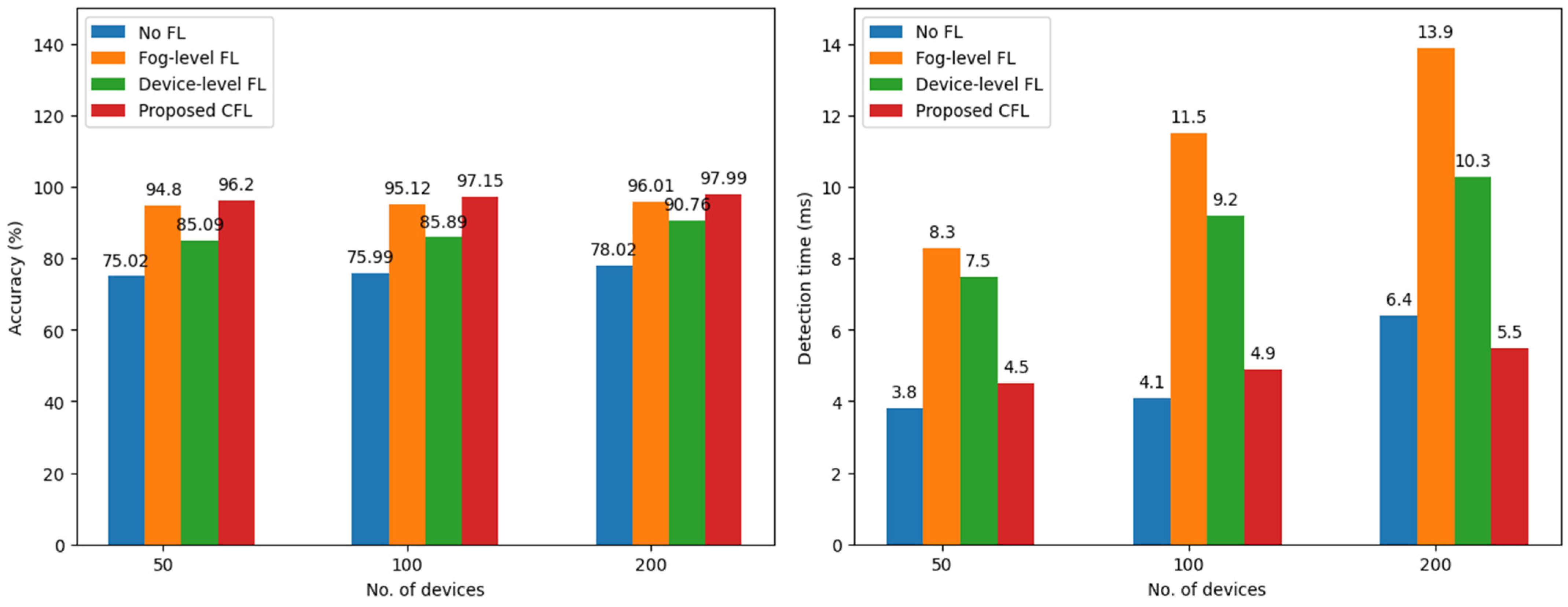
In this experiment, we test the scalability of the proposed CFL with the other methods. We increased the CFL size to 100 and 200 devices measure accuracy and detection time over 10 rounds. The experiment has been executed 10 times for each method size in each round. For devices involvements, we use the same involvements of S1 as in Table 3. Figure 9 shows average accuracy and detection time; the proposed CFL shows consistent performance stability as the number of devices increases. Compared with the other methods, our CFL outperforms them in terms of scalability. This experiment proves that the proposed CFL is scalable and stable with a large number of devices in FL. Therefore, as the number of devices in FL increases, the model learns all types of attacks more accurately. Although the CFL is constant, accuracy drops below 95% when the number of devices exceeds 200.

In summary, our proposed system can achieve performance similar to a model trained on global data by leveraging the collaborative efforts of models trained on localized data. The proposed IDS-CFL has achieved the minimum of the objective function. This is because IDS-CFL optimizes the detection accuracy and detection time as the objective function. However, the proposed CFL model with DCGAN had the highest detection time among the CNN and GAN models. It achieves the best accuracy among the other models. Thus, it achieves a tradeoff between accuracy and detection time. Although the proposed CFL achieves acceptable performance, it has limitations, such as maintaining consistent accuracy and real-time performance. The distribution and heterogeneity of IoT data across different device capabilities makes it challenging to maintain constant accuracy. Although the proposed CFL is trained on a non-IID dataset, it needs to be tested on real-time data to prove its effectiveness.

6. Conclusions

In this paper, a distributed IDS-based collaborative FL (IDS-CFL) was proposed to detect attacks in 6G-IoT networks. The collaboration is performed among three levels: device, fog, and cloud levels to reduce communication latency. A Deep Convolutional Generative Adversarial Network (DCGAN) model was proposed to improve detection accuracy and enable faster processing across different learning levels. To evaluate the performance of our system, we conducted different experiments comparing the proposed system with distributed and centralized methods. To demonstrate the effectiveness of the DCGAN model, we compared it with other models, such as a basic Convolutional Neural Network (CNN) and Generative Adversarial Network (GAN). The performance of the proposed system was evaluated on a recent Edge-IIoTest dataset, achieving the highest performance with 96.20% accuracy and 4.5 ms detection time. As future work, we aim to address the limitations. We will evaluate the proposed system in real 6G-IoT scenarios with advanced convergence strategy to maintain accuracy constant, using real-time data.

References

1. Tera, S.P.; Chinthaginjala, R.; Pau, G.; Kim, T.H. Towards 6G: An Overview of the Next Generation of Intelligent Network Connectivity. IEEE Access 2024, 13, 925–961. [Google Scholar] [CrossRef] [Scilit]
2. Nguyen, D.C.; Ding, M.; Pathirana, P.N.; Seneviratne, A.; Li, J.; Niyato, D.; Dobre, O.; Poor, H.V. 6G Internet of Things: A Comprehensive Survey. IEEE Internet Things J. 2021, 9, 359–383. [Google Scholar] [CrossRef] [Scilit]
3. Junior, E.E. Systematic Review of 6G-IoT Privacy Risks, Emerging Threats, Mitigation Strategies, and Cybersecurity. SSRN Electron. J. 2025, 19, 180–190. [Google Scholar] [CrossRef] [Scilit]
4. Assiri, M. Artificial intelligence-based intrusion detection and secure communication model for sustainable 6G-IoT networks. Sci. Rep. 2026, 16, 12662. [Google Scholar] [CrossRef] [Scilit] [PubMed]
5. Wu, Y.; Chen, J.; Lei, T.; Yu, J.; Hossain, M.S. Web 3.0 security: Backdoor attacks in federated learning-based automatic speaker verification systems in the 6G era. Future Gener. Comput. Syst. 2024, 160, 433–441. [Google Scholar] [CrossRef] [Scilit]
6. Edegbe, G.N.; Acheme, S. A systematic review of centralized and decentralized machine learning models: Security concerns, defenses and future directions. NIPES-J. Sci. Technol. Res. 2024, 6, 161–175. [Google Scholar] [CrossRef]
7. Chen, K.; Liu, Y. Toward Privacy-Preserving AI Standards for Federated Learning in 6G-Enabled Digital Twin Environments. IEEE Commun. Stand. Mag. 2025, 10, 265–272. [Google Scholar] [CrossRef] [Scilit]
8. de Alwis, C.; Aouedi, O.; Xu, J.; Wang, S.; Siriwardhana, Y.; Hewa, T.; Zeydan, E.; Sandeepa, C.; Liyanage, M. Federated Learning for 6G Security: A Survey on Threats, Solutions, and Research Directions. IEEE Commun. Surv. Tutor. 2026, 28, 4883–4914. [Google Scholar] [CrossRef] [Scilit]
9. Tomkos, I.; Klonidis, D.; Pikasis, E.; Theodoridis, S. Toward the 6G network era: Opportunities and challenges. IT Prof. 2020, 22, 34–38. [Google Scholar] [CrossRef] [Scilit]
10. Creswell, A.; White, T.; Dumoulin, V.; Arulkumaran, K.; Sengupta, B.; Bharath, A.A. Generative adversarial networks: An overview. IEEE Signal Process. Mag. 2024, 35, 53–65. [Google Scholar] [CrossRef] [Scilit]
11. Wu, Y.; Nie, L.; Wang, S.; Ning, Z.; Li, S. Intelligent Intrusion Detection for Internet of Things Security: A Deep Convolutional Generative Adversarial Network-enabled Approach. IEEE Internet Things J. 2021, 10, 3094–3106. [Google Scholar] [CrossRef] [Scilit]
12. Saeed, M.M.; Saeed, R.A.; Gaid, A.S.A.; Mokhtar, R.A.; Khalifa, O.O.; Ahmed, Z.E. Attacks Detection in 6G Wireless Networks Using Machine Learning; IGI Global: Hershey, PA, USA, 2023; pp. 6–11. [Google Scholar] [CrossRef] [Scilit]
13. Rao, V.A.; Rao, R.; Hota, C. Anomaly detection in wireless body area networks using generative adversarial networks. In Proceedings of the 2024 IEEE International Conference on Industry 4.0, Artificial Intelligence, and Communications Technology (IAICT), Bali, Indonesia, 4–6 July 2024. [Google Scholar]
14. Lin, C.-Y.; Chen, C.-Z. Inpainting-based anomaly detection system with self-supervised learning. In Proceedings of the 2024 IEEE International Conference on Industry 4.0, Artificial Intelligence, and Communications Technology (IAICT), Bali, Indonesia, 4–6 July 2024. [Google Scholar]
15. Hinojosa-Palafox, E.A.; Rodríguez-Elías, O.M.; Pacheco-Ramírez, J.H.; Hoyo-Montaño, J.A.; Pérez-Patricio, M.; Espejel-Blanco, D.F. A Novel Unsupervised Anomaly Detection Framework for Early Fault Detection in Complex Industrial Settings. IEEE Access 2024, 12, 181823–181845. [Google Scholar] [CrossRef] [Scilit]
16. Zhang, J.; Luo, C.; Jiang, Y.; Min, G. Decentralized Federated Learning for Intrusion Detection in 6G-based UxV Networks. IEEE Veh. Technol. Mag. 2025, 20, 83–93. [Google Scholar] [CrossRef] [Scilit]
17. Garroppo, R.G.; Giardina, P.G.; Landi, G.; Ruta, M. Trustworthy AI and Federated Learning for Intrusion Detection in 6G-Connected Smart Buildings. Future Internet 2025, 17, 191. [Google Scholar] [CrossRef] [Scilit]
18. Korba, A.A.; Sebaa, S.; Mabrouki, M.; G-Doudane, Y.; Benatchba, K. A Life-long Learning Intrusion Detection System for 6G-Enabled IoV. In Proceedings of the 2024 International Wireless Communications and Mobile Computing (IWCMC); IEEE: New York, NY, USA, 2024; pp. 1773–1778. [Google Scholar] [CrossRef] [Scilit]
19. Ma, X.; Hu, J.; Liang, S.; Wu, Y. Federated Learning and Resource-Aware Graph Neural Network for Intrusion Detection in 6G-IoT Driven Healthcare System. IEEE Internet Things J. 2025, 13, 7749–7761. [Google Scholar] [CrossRef] [Scilit]
20. Jayarajan, J.; Mahalingam, N.; Seng, Y.K. Empowering Smart Grid Security: Towards Federated Learning in 6G-Enabled Smart Grids using Cloud. Res. Sq. 2024; preprint. [CrossRef] [Scilit] [PubMed]
21. Prathiba, S.B.; Raja, G.; Anbalagan, S.; Gurumoorthy, S.; Kumar, N.; Guizani, M. Cybertwin-Driven Federated Learning Based Personalized Service Provision for 6G-V2X. IEEE Trans. Veh. Technol. 2022, 71, 4632–4641. [Google Scholar] [CrossRef] [Scilit]
22. Alatawi, M.N. SAFEL-IoT: Secure Adaptive Federated Learning with Explainability for Anomaly Detection in 6G-Enabled Smart Industry 5.0. Electronics 2025, 14, 2153. [Google Scholar] [CrossRef] [Scilit]
23. Kianpisheh, S.; Taleb, T. Collaborative Federated Learning for 6G With a Deep Reinforcement Learning Based Controlling Mechanism: A DDoS Attack Detection Scenario. IEEE Trans. Netw. Serv. Manag. 2024, 21, 4731–4749. [Google Scholar] [CrossRef] [Scilit]
24. Sedjelmaci, H.; Kheir, N.; Boudguiga, A.; Kaaniche, N. Cooperative and smart attacks detection systems in 6G-enabled Internet of Things. In Proceedings of the ICC 2022-IEEE International Conference on Communications, Seoul, Republic of Korea, 16–20 May 2022; Available online: https://ieeexplore.ieee.org/abstract/document/9838338/ (accessed on 21 September 2023).
25. Luo, Y.; Chen, X.; Sun, H.; Li, X.; Ge, N.; Feng, W.; Lu, J. Securing 5G/6G IoT Using Transformer and Personalized Federated Learning: An Access-Side Distributed Malicious Traffic Detection Framework. IEEE Open J. Commun. Soc. 2024, 5, 1325–1339. [Google Scholar] [CrossRef] [Scilit]
26. El Houda, Z.A.; Naboulsi, D.; Kaddoum, G. A Privacy-Preserving Collaborative Jamming Attacks Detection Framework Using Federated Learning. IEEE Internet Things J. 2024, 11, 12153–12164. [Google Scholar] [CrossRef] [Scilit]
27. Faris, H.; Aljarah, I.; Al-Betar, M.A.; Mirjalili, S. Grey wolf optimizer: A review of recent variants and applications. Neural Comput. Appl. 2017, 30, 413–435. [Google Scholar] [CrossRef] [Scilit]
28. Ferrag, M.A.; Friha, O.; Hamouda, D.; Maglaras, L.; Janicke, H. Edge-IIoTset: A New Comprehensive Realistic Cyber Security Dataset of IoT and IIoT Applications for Centralized and Federated Learning. IEEE Access 2022, 10, 40281–40306. [Google Scholar] [CrossRef] [Scilit]
29. Abunada, M.; Belhaouari, S.B.; Bensmail, H. Synthetic Minority Oversampling for Imbalanced Time Series Classification Based on Path Signature. Appl. Sci. 2026, 16, 4451. [Google Scholar] [CrossRef] [Scilit]
30. Trindade, S.; da Fonseca, N.L.S. Multicriteria Scoring for Cluster and Client Selection in Heterogeneous Hierarchical Federated Learning. IEEE Internet Things J. 2026, 13, 16763–16779. [Google Scholar] [CrossRef] [Scilit]
31. Kaur, R. Generative Adversarial Network (GANs) for Image Generation or Data Augmentation. Int. J. Sci. Archit. Technol. Environ. 2025, 3, 509–517. [Google Scholar] [CrossRef] [Scilit]
Figure 1. Distributed attack model in 6G-IoT network.
Computers 15 00644 g001
Figure 2. Collaborative FL architecture.
Computers 15 00644 g002
Figure 3. DCGAN architecture.
Computers 15 00644 g003
Figure 4. Data distribution (a) before and (b) after data balancing.
Computers 15 00644 g004
Figure 5. Detection time comparison in (a) S1 and (b) S2.
Computers 15 00644 g005
Figure 6. Methods performance comparison in (a) S1 and (b) S2.
Computers 15 00644 g006
Figure 7. Detection time of CNN, GAN, and DCGAN in CFL.
Computers 15 00644 g007
Figure 8. Performance of CNN, GAN, and DCGAN in CFL.
Computers 15 00644 g008
Figure 9. Scalability performance.
Computers 15 00644 g009