Explainable Deep Kernel Learning for Interpretable Automatic Modulation Classification

Abstract

Modern wireless communication systems increasingly rely on Automatic Modulation Classification (AMC) to enhance reliability and adaptability, especially in the presence of severe signal degradation. However, despite significant progress driven by deep learning, many AMC models still struggle with high computational overhead, suboptimal performance under low-signal-to-noise conditions, and limited interpretability, factors that hinder their deployment in real-time, resource-constrained environments. To address these challenges, we propose the Convolutional Random Fourier Features with Denoising Thresholding Network (CRFFDT-Net), a compact and interpretable deep kernel architecture that integrates Convolutional Random Fourier Features (CRFFSinCos), an automatic threshold-based denoising module, and a hybrid time-domain feature extractor composed of CNN and GRU layers. Our approach is validated on the RadioML 2016.10A benchmark dataset, encompassing eleven modulation types across a wide signal-to-noise ratio (SNR) spectrum. Experimental results demonstrate that CRFFDT-Net achieves an average classification accuracy that is statistically comparable to state-of-the-art models, while requiring significantly fewer parameters and offering lower inference latency. This highlights an exceptional accuracy–complexity trade-off. Moreover, interpretability analysis using GradCAM++ highlights the pivotal role of the Convolutional Random Fourier Features in the representation learning process, providing valuable insight into the model’s decision-making. These results underscore the promise of CRFFDT-Net as a lightweight and explainable solution for AMC in real-world, low-power communication systems.

1. Introduction

Automatic Modulation Classification (AMC) is a cornerstone technology that enables a receiver to recognize a signal’s modulation scheme automatically, without recourse to side-channel information. It functions as a pivotal intermediary process between signal detection and subsequent demodulation [1], making it indispensable for adaptive and intelligent communication systems. This application is extensively employed in both cooperative and non-cooperative communication situations to address significant operational imperatives such as dynamic spectral management for cognitive radio networks [2], robust signal recovery in degraded channel conditions [3], and sophisticated interference detection and characterization [4]. In cooperative communication, where network nodes assist each other by sharing information, AMC facilitates seamless interoperability and enhances overall system performance, boosting metrics like reliability and throughput [5]. Conversely, in non-cooperative communication, nodes must operate independently and without collaboration. This paradigm is common in adversarial or competitive environments, where AMC becomes a critical tool for autonomous signal identification and interference management, posing substantially greater challenges for robust implementation [6]. The fundamental importance of AMC, therefore, lies in its potential to significantly enhance the efficiency and dependability of communication. As we delve into the technical challenges, however, it becomes clear that AMC’s effectiveness is contingent upon overcoming several critical barriers, including high computational overhead, performance degradation in low-power or low-SNR regimes, and the lack of transparency in complex models.

First, one of the most critical operational hurdles arises in low-SNR conditions and complex channel environments, where the distinguishing features between modulation formats become obscured, causing the accuracy of AMC models to decrease significantly [7]. These adverse conditions frequently result in erroneous classifications, directly undermining the reliability of communication systems as a performance degradation that is especially untenable in critical applications such as emergency response communications, where unwavering robustness is paramount [8]. Second, the drive to overcome these performance limitations has led to powerful but computationally intensive deep learning (DL) models, whose deployment on embedded systems poses a significant challenge due to high computational demands [9]. Many state-of-the-art DL models are parameter-heavy, making their implementation impractical on hardware with constrained processing power and memory, a typical characteristic of edge, mobile, and IoT devices [10]. Also, this reliance on complex architectures introduces a third fundamental issue: a pronounced lack of interpretability. The inherent “black-box” nature of these models curtails their applicability and trustworthiness, leaving users and developers uncertain about the decision-making logic. The latter is a critical flaw when diagnosing misclassifications that occur under poor signal quality, thereby impeding model validation and user confidence [11]. While saliency-based methods like Class Activation Mapping (CAM) and its variants provide valuable visual explanations, their reliability and faithfulness have been subjects of critical evaluation. Seminal works have highlighted that such gradient-based methods can be misleading or sensitive to perturbations that are irrelevant to the model’s decision [12,13]. State-of-the-art research in Explainable AI (xAI) has since moved towards more robust techniques that explore causal relationships in model predictions [14] or uncover complex statistical dependencies between features [15]. However, these advanced methods often introduce significant computational complexity. In line with our objective of developing a lightweight and practical solution, our work employs a well-established CAM-based approach to provide efficient, first-level interpretability.

Regarding this, AMC techniques have traditionally been categorized into two main paradigms: likelihood-based (LB) and feature-based (FB) approaches. Each paradigm offers unique strengths while addressing different aspects of the challenges posed by modern wireless communication systems [16]. LB methods operate by evaluating the likelihood function of a received signal and comparing it against predefined thresholds to determine the most probable modulation scheme [17]. While theoretically optimal under idealized conditions, LB approaches are highly sensitive to model inaccuracies and typically degrade in performance under unknown channel conditions or in the presence of transmitter–receiver mismatches [18]. Additionally, they demand significant computational resources and require precise channel state information, which limits their feasibility in real-time or resource-constrained environments [19]. On the other hand, FB approaches circumvent the need for channel models by extracting hand-engineered features from the received signal, such as higher-order statistics (HOSs), cyclostationary properties, or power spectral density, and using these for classification [20,21,22]. While feature-based methods tend to offer greater resilience to channel uncertainty, they come with notable drawbacks. Specifically, they depend heavily on expert knowledge for manual feature engineering, lack end-to-end learning capabilities, and often struggle to generalize effectively across different noise levels, fading conditions, and modulation schemes [23].

The fundamental constraints of LB and FB methods have catalyzed a significant shift towards data-driven solutions, with DL approaches emerging as the dominant alternative [24]. DL models have increasingly surpassed their traditional counterparts by operating on a fundamentally different philosophy: they learn the complex mapping from signal to modulation class directly, thereby bypassing the need for explicit channel models or manual feature extraction [25]. This process endows DL-based AMC models with superior adaptability and resilience; they can autonomously learn to be invariant to noise and channel distortions that would confound conventional techniques. Furthermore, their capacity to learn a hierarchy of discriminative representations directly from raw signal data unlocks a level of performance that was previously unattainable [26]. Then, DL is a more scalable and powerful framework, uniquely suited to delivering the high-accuracy and robust AMC performance demanded by modern communication systems [27].

Research in DL-based AMC has largely been driven by advancements in convolutional neural network (CNN) architectures, with efforts focused on three key areas: maximizing performance, optimizing for efficiency, and developing hybrid models. Early work prioritized raw accuracy, as demonstrated by the complex-valued CNN in [28], which processed two-dimensional in-phase and quadrature (I/Q) data streams to yield a remarkable performance improvement of approximately 30% over single I/Q models, albeit at the cost of a large parameter count. Subsequently, a strong research thrust emerged to address computational efficiency. The PET-CGDNN system [29] exemplified this by using smaller kernel sizes and fewer feature maps to maintain high accuracy with only 71.800 parameters. This trend toward lightweight design is also evident in models like SCNN [30] (96.000 parameters) and the highly compact ULNN [31], which uses an attention mechanism and a lightweight backbone to operate with a mere 8.825 parameters, making it ideal for resource-constrained deployments. A third avenue of innovation involves hybrid architectures that combine spatial and temporal feature extraction. The MCLDNN model [32] integrated CNNs with Long Short-Term Memory (LSTM) units to improve classification accuracy. Similarly, the TDRNN model [33] fuses a threshold denoise (TD) module with an RNN to meet the stringent requirements of 6G networks. Collectively, these studies demonstrate significant progress in optimizing the performance–complexity trade-off. Still, they consistently lack interpretability analyses, and the opaque, overparameterized nature of deep models continues to present challenges in understanding prediction outcomes [34].

Recent research has increasingly explored the use of kernel approximations to enrich CNNs with nonlinearity and inductive biases while avoiding the quadratic costs of exact kernel methods. One notable direction has been the integration of Random Fourier Features (RFFs) into convolutional architectures. For example, Slim-RFFNet [35] introduces a convolutional backbone that leverages RFFs for image classification. However, its formulation relies on the phase-shift estimator. A second line of work uses RFFs not as convolutional operators but as auxiliary embeddings to augment deep learning architectures. In [36], for instance, authors incorporate RFF embeddings into standard networks for biomedical segmentation tasks, showing improvements in accuracy and interpretability through class activation maps. Nevertheless, these approaches treat RFFs as feature augmentations appended to conventional architectures rather than as convolutional layers that approximate a shift-invariant kernel. Parallel to these developments, a growing body of research has focused on spectral and Fourier-based convolutional layers. Han et al. [37] propose Fourier CNNs, where convolution is carried out directly in the frequency domain using FFT-based transformations. More recently, Harper et al. [38] extend this line with CF-Convs, learning continuous convolutional kernels in the Fourier domain. These approaches leverage spectral representations to improve efficiency or expressiveness, yet they are not explicitly designed as kernel approximations via Monte Carlo sampling from spectral measures. In addition, modern work has highlighted the impact of feature design on the effectiveness of random features. Likhosherstov et al. [39] propose Chefs’ Random Tables, introducing non-trigonometric random features that improve approximations for certain kernels, such as the softmax. This reinforces the importance of choosing estimators carefully, since the variance and practicality of the approximation are strongly tied to the feature map adopted. Against this background, the novelty of our proposal lies in being, to the best of our knowledge, the first convolutional RFF layer that instantiates the sine–cosine estimator inside a convolutional operator.

Here, we present the Convolutional Random Fourier Features with Denoising Thresholding Network (CRFFDT-Net), a deep kernel learning model for AMC that is engineered to be both lightweight and interpretable. The model’s primary objective is to address the critical performance–complexity trade-off. It is engineered to achieve a classification accuracy that is on par with much larger, state-of-the-art models but with a minimal computational footprint, making it both lightweight and interpretable. This is accomplished through an innovative Convolutional Random Fourier Features (CRFFs) technique that allows us to reduce the parameter count and increase interpretability while maintaining high classification performance. CRFFDT-Net builds upon our foundational work in [40], extending it through four main stages:

–

An enhanced convolutional RFF mechanism leveraging kernel functions to extract salient features from I/Q signals;

–

A threshold denoising stage based on the Residual Shrinkage Building Unit (RSBU) architecture to improve signal fidelity;

–

A compact time-domain feature extraction module, which combines a CNN with a Gated Recurrent Unit (GRU) before a final dense neural network classification layer;

–

A Class Activation Map (CAM)-based approach to reveal discriminative input features learned by the model across varying SNR levels.

Through this integrated design, our model delivers high modulation classification accuracy with reduced computational demands. Remarkably, our main contribution is the novel implementation of a convolutional layer performing kernel-based mapping via Random Fourier Features. By incorporating both sine and cosine transforms, this CRFFSinCos (Convolutional Random Fourier Features Sine–Cosine) layer extends traditional RFF methods, leveraging the full spectrum of Fourier components to significantly improve the model’s ability to capture and represent complex input patterns for AMC tasks under challenging SNR scenarios.

The agenda is as follows: Section 2 presents the materials and methods. Next, Section 3 depicts the experimental setup and configuration of the proposed network. Section 4 shows the results obtained and the discussion. Finally, Section 5 describes the concluding remarks.

2. Materials and Methods

2.1. Automatic Modulation Classification (AMC)

The objective of AMC is to identify the modulation scheme of a received signal from its raw time-series data. The received complex baseband signal, denoted as $r\left(t\right)\in \mathbb{C}$, can be expressed in terms of its in-phase (I) and quadrature (Q) components:

$$r\left(t\right)=r_I\left(t\right)+j{r}_Q\left(t\right),$$

(1)

where $r_I\left(t\right),r_Q\left(t\right)\in \mathbb{R}$ are real-valued functions of time, and $j=\sqrt{-1}$ is the imaginary unit. In a digital communication system, this continuous signal is sampled at discrete time instances, yielding a sequence of complex samples. For our purposes, we consider a frame of L such samples, ${\left\{r\left[l\right]\right\}}_{l=1}^L$, where $r\left[l\right]\in \mathbb{C}$.

To process these complex samples within a real-valued deep learning framework, we decompose them into their I and Q components. This results in a two-channel, real-valued input matrix $X\in {\mathbb{R}}^{2\times L}$, which serves as the input to our classification model:

$$X=\left(\begin{array}{c}Re\left[r\right[1],\dots ,r[L\left]\right]\\ Im\left[r\right[1],\dots ,r[L\left]\right]\end{array}\right).$$

(2)

Here, the first row of X contains the sequence of in-phase components, and the second row contains the sequence of quadrature components.

The problem can then be formally stated as learning a mapping function $f:{\mathbb{R}}^{2\times L}\to \mathcal{M}$, where $\mathcal{M}$ is the finite set of M possible modulation classes (e.g., BPSK, QAM16, etc.). Our proposed deep learning model, CRFFDT-Net, is designed to approximate this function. Given an input signal matrix X and the model parameters $\theta$, the network outputs a vector of class probabilities. The predicted modulation class, $\widehat{m}\in \mathcal{M}$, is determined by selecting the class with the highest posterior probability:

$$\widehat{m}=\underset{m\in \mathcal{M}}{argmax}f\left(m\right|X;\theta ),$$

(3)

where $f\left(m\right|X;\theta )$ represents the model’s predicted probability for class m given the input X and learned parameters $\theta$. The model’s parameters are optimized by minimizing a suitable loss function (e.g., categorical cross-entropy) between the predicted probabilities and the true modulation class labels over a training dataset.

2.2. Enhanced Signal Representation via Convolutional Random Fourier Features

To address the computational demands of conventional deep learning models, our architecture incorporates a lightweight and interpretable feature extraction module. This module is founded on a principled approximation of kernel methods, specifically a convolutional variant of Random Fourier Features (RFFs). This approach replaces standard learned convolutional filters with a compact set of randomized projections derived from kernel theory, enabling efficient and robust signal representation. The following exposition details the theoretical progression from kernel methods to our specific implementation.

Kernel methods offer a robust framework for nonlinear learning by implicitly mapping data into a high-dimensional Reproducing Kernel Hilbert Space (RKHS), where linear operations can capture complex relationships [41]. Their practical application, however, is often limited by the $O\left(N^2\right)$ complexity required to compute the Gram matrix for N samples. The RFF framework, proposed by Rahimi and Recht [42], circumvents this limitation for the broad class of shift-invariant kernels, where $k(x,y)=k(x-y)$.

The theoretical basis for this approximation is Bochner’s theorem [43], which establishes that any such kernel can be expressed as the expectation of a random complex exponential over the kernel’s power spectrum, $p\left(\omega \right)$:

$$k(x-y)={\mathbb{E}}_{\omega \sim p\left(\omega \right)}\left[e^{i{\omega }^{\top }(x-y)}\right].$$

(4)

Rahimi and Recht proposed two distinct, unbiased Monte Carlo estimators for this expectation. The first, which we denote as $\widehat{z}\left(x\right)$, uses a random phase shift b:

$$\widehat{z}\left(x\right):=\sqrt{{\displaystyle \frac{2}{D}}}{\left[cos({\omega }_1^{\top }x+b_1),\dots ,cos({\omega }_D^{\top }x+b_D)\right]}^{\top },$$

(5)

where ${\omega }_i\stackrel{iid}{\sim }p\left(\omega \right)$ and $b_i\stackrel{iid}{\sim }\mathrm{Unif}[0,2\pi ]$. The second, denoted as $\tilde{z}\left(x\right)$, uses a deterministic trigonometric expansion:

$$\tilde{z}\left(x\right):=\sqrt{{\displaystyle \frac{1}{D}}}{\left[cos\left({\omega }_1^{\top }x\right),sin\left({\omega }_1^{\top }x\right),\dots ,cos\left({\omega }_D^{\top }x\right),sin\left({\omega }_D^{\top }x\right)\right]}^{\top },$$

(6)

where the dimensionality of the feature space is $2D$. While both formulations lead to valid kernel approximations, they are not equivalent in quality. Sutherland and Schneider [44] provided a rigorous analysis demonstrating that the estimator based on $\tilde{z}\left(x\right)$ (Equation (6)) exhibits strictly lower variance than the one based on $\widehat{z}\left(x\right)$ for the ubiquitous Gaussian kernel. The phase-shifted variant introduces additional noise, whereas the sine–cosine expansion is a more direct and stable estimator. Consequently, we adopt the theoretically superior sine–cosine formulation as the foundation for our method.

To apply the RFF framework to structured grid data, such as I/Q signals, it is beneficial to incorporate the strong inductive biases of convolutional operators, namely translation-equivariance and locality. While prior work has explored convolutional variants of RFFs, such as in [45], these have typically been based on the less optimal phase-shifted embedding (Equation (5)). Our novel contribution is the development of a convolutional layer founded on the lower-variance sine–cosine embedding (Equation (6)).

Our proposed Convolutional Random Fourier Features Sine–Cosine (CRFFSinCos) layer achieves this by substituting the inner product ${\omega }^{\top }x$ with a standard convolution operation. Implemented as ‘ConvRFF_SinCos’, it operates on the following principles:

–

Randomized Filter Basis: The layer’s convolutional filters, denoted as W, are established a priori by drawing samples from the spectral distribution $p\left(\omega \right)$ of a chosen kernel (e.g., a Gaussian distribution for an RBF kernel). These filters can either remain fixed, serving as a static random basis, or be fine-tuned via backpropagation.

–

Convolutional Projection and Sine–Cosine Mapping: The projection of an input tensor X onto the random frequency basis is performed by the convolution $X\ast W$. In direct correspondence with the formulation in Equation (6), the layer computes both sine and cosine transformations of the projected output. These two sets of feature maps are subsequently concatenated along the channel axis:

$$\begin{array}{cc}\hfill F_{cos}& =cos\left(\right(X\ast W)/s)\hfill \end{array}$$

(7)

$$\begin{array}{cc}\hfill F_{sin}& =sin\left(\right(X\ast W)/s)\hfill \end{array}$$

(8)

$$\begin{array}{cc}\hfill F_{out}& =\mathrm{concat}[F_{sin},F_{cos}],\hfill \end{array}$$

(9)

where s is the scaling hyperparameter, ‘kernel_scale’, which normalizes the projected values before the trigonometric mapping.

–

Stochastic Approximation Normalization: A final scaling factor of $\sqrt{1/D}$, where D is the number of output filters (‘output_dim’), is applied to the concatenated feature maps. This normalization is a theoretical requisite of the Monte Carlo formulation, ensuring that the inner product of the output features remains a consistent estimator of the target kernel.

This architectural synthesis results in a highly efficient feature extraction module. By leveraging a principled, kernel-based random projection scheme that is demonstrably superior in terms of variance, and by integrating it with the proven inductive biases of convolutional architectures, our CRFFSinCos layer provides a robust and theoretically sound method for signal representation.

2.3. Class Activation Mapping-Based Model Interpretability

Grad-CAM++ represents a key evolution in explainability methods for deep learning systems, especially for convolutional neural networks. It generates visual rationales for the predictions formulated by these models [46]. For a CNN producing class scores prior to the Softmax function, the score for class c is represented by $Y^c$. The feature maps of a chosen convolutional layer are denoted by $A^k$, with k as the index. Grad-CAM++ works by creating a weighted aggregate of these feature maps to identify regions that are pivotal to the model’s classification. The weighting coefficients ${\alpha }_{ij}^k$, at position $i,j$ in feature map k, are determined by the following equation:

$${\alpha }_{ij}^k={\displaystyle \frac{{\sum }_{a,b}\left(\frac{{\partial }^2{Y}^c}{{(\partial A_{ij}^k)}^2}\right)·\mathrm{ReLU}\left(\frac{\partial Y^c}{\partial A_{ij}^k}\right)}{{\sum }_{a,b}\frac{{\partial }^2{Y}^c}{{(\partial A_{ij}^k)}^2}}}.$$

(10)

where the ReLU (rectified linear unit) is the activation function used to ensure consideration is limited to features that positively affect the class score. The final class activation map for class c, is produced by integrating these weights with their corresponding feature maps:

$$L_{\text{Grad-CAM}++}^c=\mathrm{ReLU}\left(\sum _k{\alpha }_k\sum _{i,j}\mathrm{ReLU}\left({\displaystyle \frac{\partial Y^c}{\partial A_{ij}^k}}\right)A_{ij}^k\right).$$

(11)

In this sense, the Grad-CAM++ procedure requires a forward and backward propagation through the network to compute the gradients of the class score with respect to a convolutional layer’s feature maps. These gradients are then utilized to weight the activation maps that guide the model’s prediction [47]. The final heatmap can be overlaid on the input, visually highlighting the regions the model deemed most critical for its decision-making process [48].

3. Experimental Setup

3.1. Dataset Description

We employ the well-known RadioML 2016.10A dataset, which contains 220,000 signals (https://www.deepsig.ai/datasets/, accessed on 1 May 2025). The signals are categorized across 20 distinct SNRs, holding 1000 signals per modulation type at each SNR. Regarding this, values range from $-20$ dB to $+18$ dB, and each signal has a frame length of 128 and belongs to one of 11 modulation types (classes), comprising 8 digital and 3 analog.

It is worth noting that the studied dataset is valued for its affordability and low hardware requirements. Its compact design and low computational requirements make it particularly suitable for researchers working with limited budgets or constrained access to high-performance computing resources. Due to its cost-effectiveness and minimal hardware demands, it offers a practical solution for AMC testing without the need for substantial financial or infrastructural investments. These considerations motivated our choice of the RadioML 2016.10A dataset, which offers a diverse and well-structured representation of modulation types across a wide range of SNR levels, facilitating comprehensive evaluation and benchmarking of classification approaches.

3.2. Architecture Details

Figure 1 depicts the CRFFDT-Net main blocks, comprising a CRFF layer, denoising, and hidden feature extraction with dense layers-based classification.

Our method begins with an input layer where each sample has a size of $2\times L$. In this work, we set $L=128$ to match the frame length used in the RadioML 2016.10A dataset. To address internal covariate shifts and stabilize training, batch normalization (BN) is applied to normalize the features across each sample. Following this, the input is processed by the proposed 2D CRFFSinCos layer, which comprises 16 filters (i.e., convrff). This layer employs the rectified linear unit (ReLU) as its activation function.

Then, the signal is processed by a denoising sub-network specifically designed for threshold-based denoising, which automatically estimates an optimal threshold for each input. In this study, we employ the RSBU architecture introduced in [49], which computes a channel-specific threshold parameter $\gamma \left(c\right)$ through a multi-step procedure. Initially, two convolutional layers (namely, conv2D and $conv2D_1$) are applied to the input, capturing spatial patterns that are critical for denoising and classification, while enhancing key features and attenuating noise and irrelevant information. The resulting feature map is then converted into a one-dimensional representation by taking the absolute value of the global average pooling (GAP), effectively reducing the dimensionality and the number of parameters in the subsequent fully connected (FC) layer, thereby minimizing overfitting risk. This one-dimensional vector is subsequently fed into a two-layer FC network to estimate the scaling parameter $\alpha \left(c\right)$ corresponding to the c-th neuron. To constrain $\alpha \left(c\right)$ within the interval $(0,1)$, a sigmoid function is applied, defined as follows:

$$\alpha \left(c\right)={\displaystyle \frac{1}{1+{exp}^{-z\left(c\right)}}},$$

(12)

where $z\left(c\right)$ denotes the feature corresponding to the c-th neuron. Afterward, the thresholding value $\gamma \left(c\right)$ is then computed through element-wise multiplication of $\alpha \left(c\right)$ with the absolute GAP output $\beta$:

$$\gamma \left(c\right)=\alpha \left(c\right)·\beta .$$

(13)

Next, the signal is denoised using the soft thresholding function $\delta \left(\omega \right)$, which sets values within the threshold range to zero and subtracts the threshold from values outside the range:

$$\begin{array}{c}\hfill \delta \left(\omega \right)=\left\{\begin{array}{cc}0,\hfill & \left|\omega \right|<\gamma \hfill \\ \left(\right|\omega -\gamma \left|\right)·sgn\left(\omega \right),\hfill & \left|\omega \right|\ge \gamma \hfill \end{array}\right.,\end{array}$$

(14)

where $\omega$ and $\delta \left(\omega \right)$ represent the input and output features, respectively, $\gamma$ is the learned threshold, and $sgn\left(\omega \right)$ denotes the sign function.

Following denoising, the enhanced signal is passed through a time-domain feature extraction module designed to capture both local and sequential patterns that are critical for accurate modulation classification. This module initially applies two convolutional layers (i.e., conv2d_2 and conv2d_3), each followed by a ReLU activation function, enabling the extraction of increasingly abstract spatial features from the denoised input. These convolutional operations facilitate the modeling of local dependencies within the time-series data, emphasizing salient signal structures. Subsequently, the output of the convolutional stack, originally a four-dimensional tensor, must be reshaped to meet the input requirements of the recurrent layer. Therefore, a Reshape operation is applied to convert the tensor into a three-dimensional form, structured as $(\mathrm{batch}\mathrm{size},\mathrm{timesteps},\mathrm{features})$, which is compatible with recurrent architectures.

At last, a Gated Recurrent Unit (GRU) layer with 64 hidden units is employed. The GRU is specifically chosen for its ability to model temporal dependencies efficiently, offering a lighter alternative to traditional LSTM cells while maintaining competitive performance.

Also, the proposed architecture includes a fully connected layer with 11 units, with each corresponding to one of the 11 modulation types in the dataset, to perform modulation classification. To generate probability distributions for these classes, the Softmax activation function is applied. This function normalizes the outputs from the previous layers, ensuring that the sum of the predicted probabilities equals 1. Such normalization enhances prediction accuracy and facilitates identifying the most likely category for a given input.

Additionally, we utilize the Adam optimizer along with the categorical cross-entropy ($CCE$) as the loss function for optimization. The $CCE$ function is expressed as follows:

$$\begin{array}{cc}\hfill L_{CCE}& =\sum _{i=1}^M{Y}_{1}log\left(Y_2\right)\hfill \end{array}$$

(15)

$$\begin{array}{cc}\hfill Y_2& =f\left(x_i\right)\hfill \end{array}$$

(16)

where $Y_1$ represents the ground truth vector, which can be encoded using one-hot encoding. $Y_2$ indicates the predicted probability vector, which corresponds to the model’s final output after the Softmax activation function is applied. M refers to the total number of modulation classes, and $x_i$ corresponds to the i-th AMC output.

3.3. Ablation Study Design

To validate the contribution and design of the CRFFSinCos layer, we compared three model variants while keeping the rest of the architecture and all hyperparameters fixed:

–

CRFFDT-Net (trainable_rff): This is the complete proposed architecture, where the randomly sampled Fourier features are fine-tuned during training.

–

fixed_rff: This is the same architecture as the full model, but the randomly sampled Fourier features in the CRFFSinCos layer are kept fixed and are not updated during backpropagation.

–

no_rff: Ths CRFFSinCos layer is replaced by a standard 2D convolutional layer with the same input/output dimensions and number of filters.

To justify the inclusion and design of our RSBU-based denoising module, we conducted a targeted ablation study to compare its performance against simpler, non-adaptive thresholding methods. In this experiment, all other components of the CRFFDT-Net backbone were held fixed—including the ConvRFF layer, all subsequent convolutional and GRU layers, the classifier, and all training parameters. The only factor changed was the thresholding operator applied within the denoising block. We evaluated the following five configurations:

–

None: An identity function, where no denoising is applied.

–

Soft Thresholding (soft-std): A standard soft thresholding function is applied using a universal, per-channel threshold ${\tau }_c=k·{\widehat{\sigma }}_c\sqrt{2log\left(HW\right)}$, where ${\widehat{\sigma }}_c$ is the estimated standard deviation of the noise in channel c, H and W are the feature map dimensions, and $k=1$.

–

Hard Thresholding (hard-std): A hard thresholding function (setting values below ${\tau }_c$ to zero) is applied using the same universal threshold.

–

Garrote Thresholding (garrote-std): A non-negative garrote thresholding function is applied, again using the same universal threshold.

–

RSBU (Adaptive): Our original proposed block, which estimates an adaptive, per-channel threshold ${\tau }_c=s_c·{\mu }_c$ where ${\mu }_c=\mathrm{GAP}\left(\right|x\left|\right)$ is derived from the input features via a BN-ReLU-MLP gate. This module then applies soft thresholding.

This setup allows for a direct comparison of our adaptive approach against both no denoising and simpler, static thresholding rules.

3.4. Quantitative Interpretability Evaluation

To further assess the interpretability of the proposed approach, we evaluated the quality of the CAMs using the deletion and insertion protocols. These perturbation-based methods test whether the regions identified as most relevant by the CAMs are indeed critical for classification. Since interpretability effects can be confounded by high noise levels, the evaluation was restricted to the highest SNR setting, where classifier predictions are most reliable and differences among architectures can be attributed to the quality of the highlighted evidence rather than random channel fluctuations.

In the deletion protocol, the 128 time steps of each signal were ranked according to their CAM scores for the true class (summed over the in-phase and quadrature components). A fraction $p\in \{0,5,10,20,40,60,80,100\}\%$ of the top-ranked indices was progressively masked with power-matched Gaussian noise. The true-class probability that was recorded as p increased, and the area under the resulting curve (AUC_del) was used as a metric: lower values correspond to CAMs that identify more causally important time steps. In the insertion protocol, the process was inverted. Starting from a fully corrupted signal, the top-$p\%$ indices were progressively restored to their original values, and the model’s probability for the true class was tracked. The corresponding area under this curve (AUC_ins) was measured, with higher values indicating more faithful CAMs.

3.5. Training and Validation Strategy

We present a method to evaluate the efficiency of CRFFDT-Net using the RadioML 2016.10A dataset. The model is trained using a single random split strategy, allocating 70% of the data for training and 30% for testing. To enhance the learning process and prevent overfitting, we incorporate an Early-Stopping mechanism along with the ReduceLearningRateOnPlateau callback, which reduces the learning rate when a monitored metric (i.e., accuracy and loss value) shows no further improvement. All experiments were performed on the Kaggle platform using GPU-enabled notebooks. Each session granted access to a single NVIDIA Tesla P100 GPU (NVIDIA Corporation, Santa Clara-US), 16 GB of VRAM, 30 GB of RAM, and 4 virtual CPUs powered by an Intel Xeon CPU @ 2.20 GHz. The entire codebase was implemented in Python 3.11.11, and all models were executed within Kaggle’s default runtime environment, with the exact package versions specified in the notebook’s dependency list. The complete source code for all experiments has been made publicly available at https://github.com/UN-GCPDS/AMC/, accessed on 1 May 2025.

4. Results and Discussion

This section presents the performance of the proposed CRFFDT-Net model in comparison with a diverse set of baseline architectures for the AMC task. The evaluation is carried out under varying noise conditions, emphasizing both quantitative metrics such as classification accuracy and model rankings across different SNRs, and qualitative aspects, including interpretability and model complexity. To ensure a comprehensive assessment, we also incorporate statistical significance tests and class-wise visualizations that highlight the model’s behavior in realistic and challenging scenarios.

4.1. Classification Performance

In Figure 2, we display the average accuracy distribution obtained by each compared model across all considered SNRs. As expected, most models tend to distinguish better between different modulations as the ratio of noise decreases, i.e., for SNR levels greater than zero. Specifically, we segment the baseline approaches among three categories, namely, CNN-based, RNN-based, and hybrid models which combine convolutional and recurrent layers (in this, we locate our proposal).

In comparison with our proposed CRFFDT-Net model, CNN-based architectures exhibit low performance since relying solely on spatial characteristics is captured by CNN layers generally [16]. Similarly, the RNN-based approaches yield low classification accuracy, however, the LSTM2 model achieves a competitive accuracy with ∼59%. Regarding the hybrid approaches, our proposed CRFFDT-Net (∼62% accuracy) achieves a performance comparable to other top-performing models like MCLDNN (∼63%) and PET-CGDNN. On the contrary, CGDNet yields the worst performance with an accuracy of ∼45%.

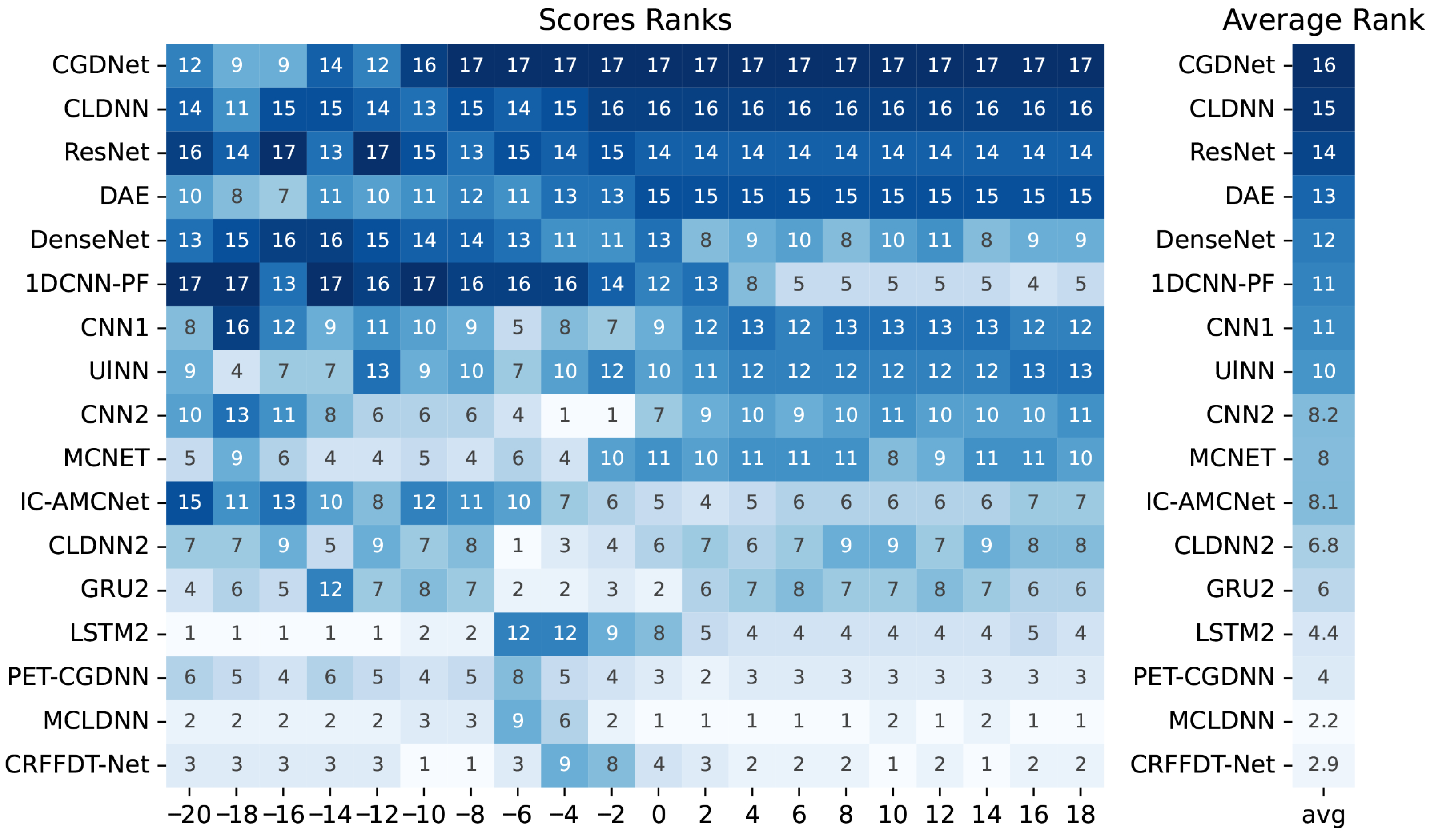
A detailed analysis of the classification results is presented in Figure 3, which shows the ranking of each model across different SNR levels (left matrix) and the corresponding average ranking (right vector). The matrix displays the rank scores for each model at each SNR level, based on their classification performance. For example, at an SNR of $-10$ dB, the proposed CRFFDT-Net ranks first, followed by the LSTM2 model in second place, and so forth.

We observe that architectures such as ResNet, DenseNet, CNN1, and CNN2, which process raw I/Q data directly as input, tend to exhibit lower performance. In contrast, 1DCNN-PF, which leverages amplitude and phase representations as input features, struggles at lower SNR levels but achieves notable improvements at higher SNRs (above 2 dB). Models such as MCNet and IC-AMCNet outperform others, benefiting from advanced mechanisms like multi-scale feature extraction in MCNet and the injection of Gaussian noise in IC-AMCNet, which enhance their ability to capture diverse signal characteristics. Recurrent models, which are capable of capturing the temporal dependencies that are inherent in wireless communication signals, generally perform better [50]. Despite their relatively simple architectures, GRU2 and LSTM2, each with only a few layers, achieve higher overall recognition accuracy. Notably, LSTM2 demonstrates superior performance at very low-SNRs (below $-10$ dB). The inclusion of a reconstruction branch in the DAE model does not appear to enhance recognition performance, as it ranks among the least accurate models evaluated. Hybrid architectures, which combine spatial and temporal feature extraction, tend to outperform single-stream models. However, their effectiveness varies significantly with architectural choices. For example, CGDNet and CLDNN show comparatively low accuracy, potentially due to their limited parameter counts. In contrast, models such as CLDNN2 and MLCDNN, which possess more parameters, perform significantly better. Notably, the proposed CRFFDT-Net mitigates the limitations of lightweight architectures by incorporating advanced feature processing techniques, such as parametric inverse transformation and a two-dimensional convolutional RFF, respectively, leading to improved recognition accuracy.

For a more comprehensive performance assessment, we supplemented our accuracy analysis by computing the macro-averaged precision, recall, and F1-score for each model, which are appropriate in our case since the dataset is perfectly balanced across both modulation classes and SNR levels. Thus, macro-averaging provides an unbiased global summary of performance without the need for weighted alternatives.

Table 1. Performance comparison of different neural network architectures for AMC. Reported values correspond to macro-averaged accuracy, precision, recall, and F1-score, which are appropriate since the dataset is perfectly balanced across both SNR levels and modulation classes. The top three results per metric are highlighted in bold.

Model	Accuracy	Precision	Recall	F1
CGDNet	0.438	0.244	0.168	0.182
CLDNN	0.500	0.230	0.171	0.182
ResNet	0.527	0.230	0.168	0.181
DAE	0.522	0.269	0.204	0.217
DenseNet	0.545	0.272	0.208	0.219
1DCNN-PF	0.544	0.349	0.288	0.299
CNN1	0.550	0.247	0.188	0.200
UINN	0.547	0.239	0.178	0.192
CNN2	0.563	0.273	0.214	0.223
MCNET	0.560	0.252	0.190	0.203
IC-AMCNet	0.563	0.274	0.215	0.227
CLDNN2	0.565	0.263	0.203	0.216
GRU2	0.569	0.261	0.200	0.217
LSTM2	0.596	0.277	0.222	0.233
PET-CGDNN	0.583	0.286	0.231	0.241
MCLDNN	0.614	0.300	0.250	0.261
CRFFDT-Net	0.609	0.277	0.219	0.216

presents the revised results, with the top three models per metric highlighted in bold. The metrics confirm the top-tier accuracy of MCLDNN, CRFFDT-Net, and LSTM2. However, they also reveal a more complex performance landscape. Notably, the 1DCNN-PF model, despite its modest accuracy, achieves the best precision, recall, and F1-score. This suggests that its architecture, which relies on explicit amplitude and phase feature extraction, excels at correctly identifying the classes it is confident about, even if it struggles more broadly. MCLDNN demonstrates its robustness by securing a top-three rank across all four metrics, solidifying its position as a strong, all-around performer. PET-CGDNN also shows high precision, indicating a low false-positive rate. Our proposed CRFFDT-Net achieves the second-highest accuracy while its other metrics remain competitive. This outcome reinforces our central claim: the primary strength of CRFFDT-Net lies in achieving top-tier accuracy with exceptional efficiency, rather than leading on every classification metric.

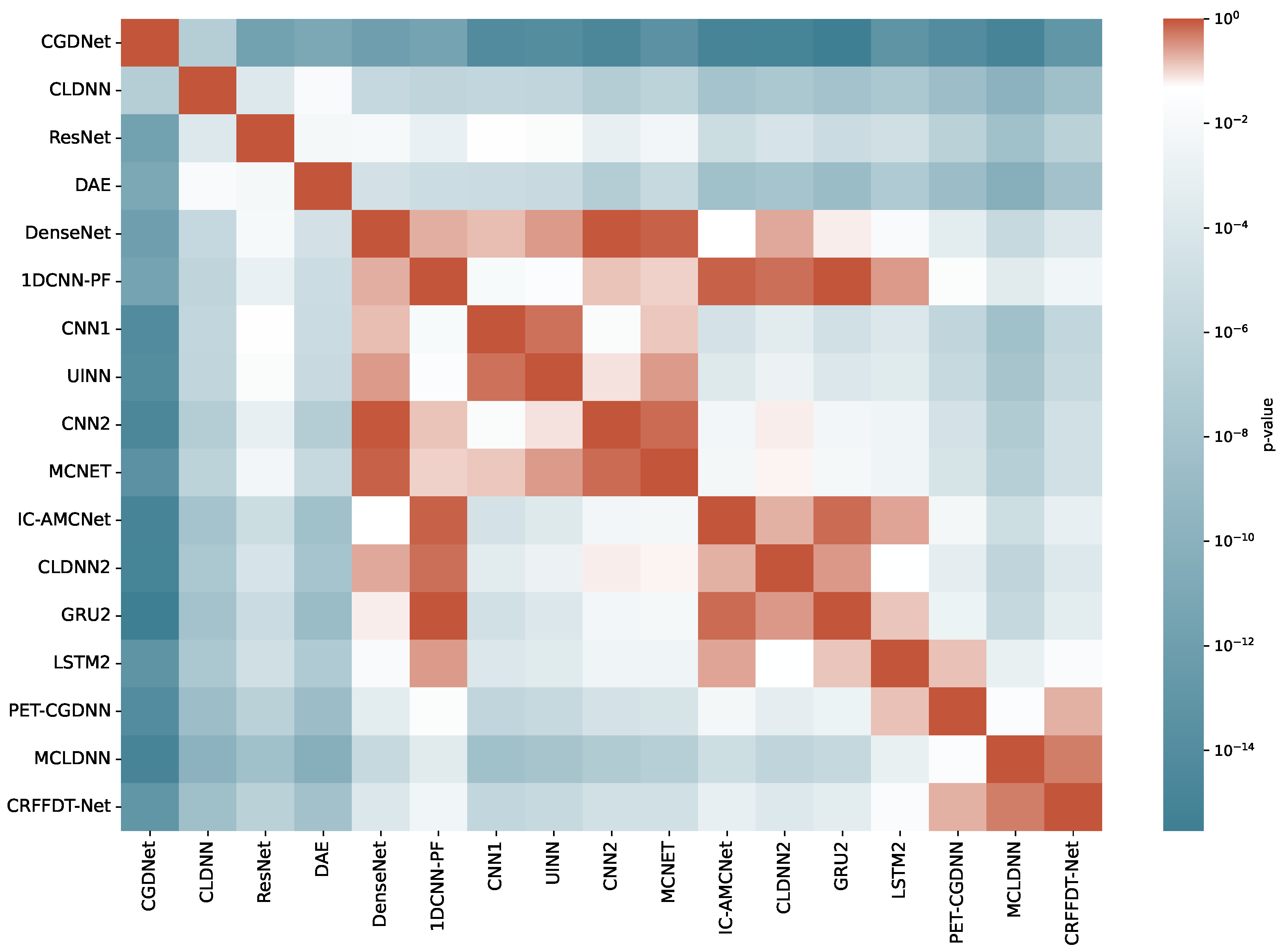
To assess the statistical significance of the similarities and differences among the obtained results, we first applied a Friedman test, considering only the SNR values above 0. The test yielded a p-value of $1.09\times {10}^{-22}$, indicating statistically significant differences among the evaluated models. To further investigate the source of these differences, we conducted pairwise t-tests, and the resulting p-values are summarized in Figure 4. From the pairwise t-test results, we observe no statistically significant differences among the higher-performing CNN-based models. Likewise, no significant differences were found among the RNN-based models, namely GRU2, LSTM2, IC-AMCNet, and CLDNN2. In contrast, our proposed model exhibits statistically significant differences when compared to all other models, except MCLDNN and PET-CGDNN.

Based on the above findings, we center our subsequent analysis on our proposed model and the two most comparable alternatives (MCLDNN and PET-CGDNN) given their similar performance profiles and the absence of statistically significant differences in the pairwise comparisons. We analyze the results under three distinct noise conditions (high, medium, and low), corresponding to SNR levels of $-18$, 0, and 18 dB, respectively. Figure 5 presents the confusion matrices for each considered noise level. In general, PET-CGDNN, MCLDNN, and our proposed model demonstrate comparable performance, exhibiting similar classification patterns across the different SNR scenarios. These observations are consistent with the outcomes of the pairwise t-tests. Under high noise conditions ($-18$ dB), all three models tend to classify a majority of signals as AM-SSB, with this tendency being most prominent in PET-CGDNN. Meanwhile, MCLDNN and CRFFDT-Net show a slight inclination to confuse instances of BPSK, CPFSK, and GFSK among each other. Notably, MCLDNN correctly classifies a significant portion of AM-DSB signals but also mislabels several WBFM samples as AM-DSB. Unlike narrowband modulations, WBFM spans a much wider frequency range and includes nonlinear phase and amplitude variations that often overlap spectrally with other modulation schemes when processed under low-SNR conditions [51]. As the SNR increases from 0 dB and 18 dB, a clear improvement in classification accuracy is observed. Nevertheless, misclassification of WBFM signals as AM-DSB persists, albeit with reduced frequency, particularly in the case of our proposed model. At these higher SNR levels, all three models encounter difficulties in distinguishing between QAM16 and QAM64; however, this issue is less severe in MCLDNN and CRFFDT-Net, especially under low noise conditions.

4.2. Model Complexity Analysis

In the context of AMC, model complexity is a critical factor that directly impacts computational efficiency and the feasibility of deployment in real-time or resource-constrained environments. While the number of trainable parameters is a common proxy for complexity, a more comprehensive assessment must also include computational cost (FLOPs) and real-world inference speed (latency), especially on embedded hardware. In this study, we conduct a comparative analysis among the state-of-the-art models, taking into account their classification accuracy and these three key complexity metrics.

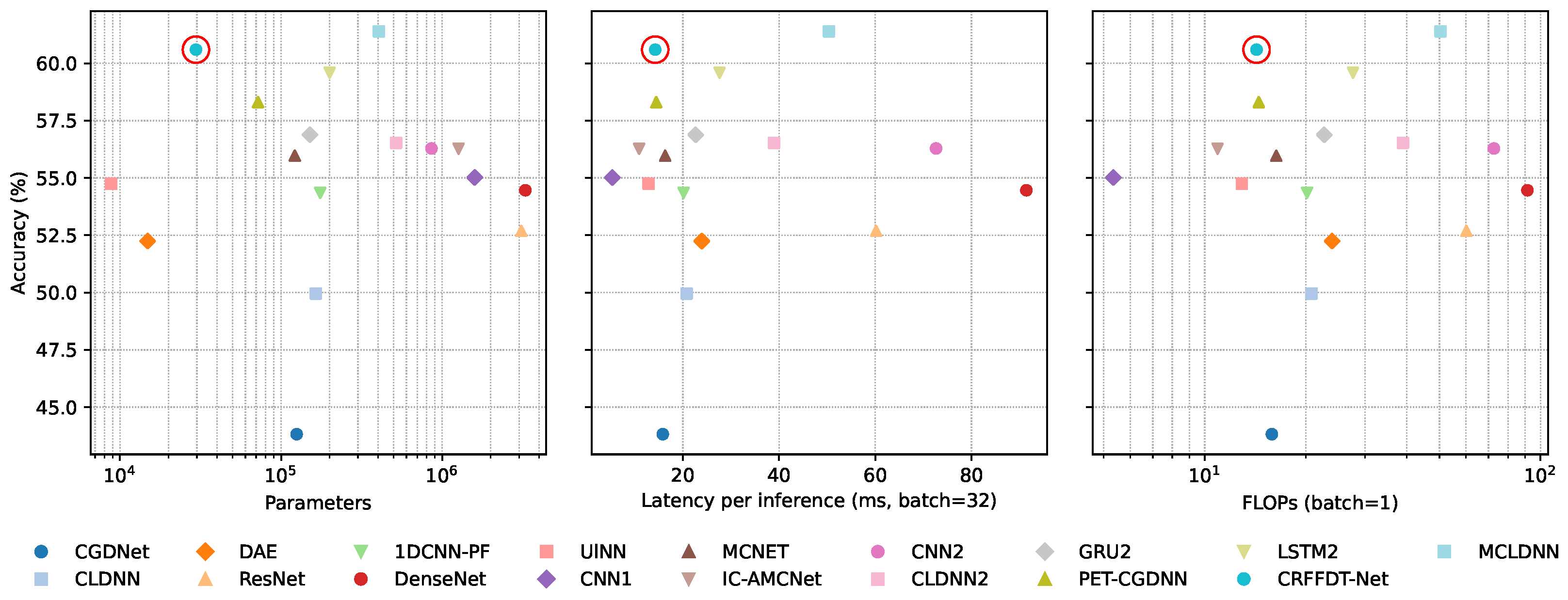
Figure 6 illustrates the trade-off between average accuracy and model complexity. As shown in the left panel, our proposed CRFFDT-Net is among the most lightweight models with approximately ∼29,000 trainable parameters. This efficiency is largely attributed to the use of RFFs, which approximates a shift-invariant kernel by projecting the input onto a compact set of random features, eliminating the need for numerous learnable convolutional filters. These projections effectively capture essential signal characteristics without requiring the training of individual filter elements, thereby significantly reducing the number of learnable parameters while maintaining strong feature discriminability [52]. More importantly, the new experimental results on computational and runtime performance provide stronger evidence of its efficiency. The right panel shows that CRFFDT-Net requires one of the lowest amounts of FLOPs per inference, significantly outperforming more complex architectures like MCLDNN and LSTM2 while achieving superior accuracy. Crucially, the middle panel presents the inference latency measured on a Jetson Nano device. Our model demonstrates a highly competitive latency of approximately 20 ms, confirming its suitability for real-time processing on resource-constrained embedded systems. Collectively, these results demonstrate that CRFFDT-Net achieves a superior balance between classification accuracy and overall complexity, making it a practical and efficient solution for real-world AMC applications.

By decomposing the input signal into sine and cosine components, the model captures both local and global variations, significantly reducing parameter overhead [53] while maintaining competitive performance. Additionally, the subsequent layers, including the threshold-based denoising module, optimize only a small number of parameters (e.g., thresholds and compact fully connected layers), avoiding the use of large weight matrices. This architectural design results in a streamlined yet effective processing pipeline, where the computational burden of feature extraction is offloaded to the RFF-based kernel approximation. Consequently, the proposed model achieves a favorable balance between classification accuracy and computational efficiency.

4.3. Ablation Study Results

To empirically validate the contribution of our proposed architectural innovations, we conducted two targeted ablation studies focusing on the CRFFSinCos layer and the threshold-based denoising module. The combined results are presented in

Table 2. Ablation study results at high SNRs (i.e., 0 db–$+18$ db), evaluating the impact of the RFF layer and the denoising module. The results validate our key architectural design choices.

Model Variant	Accuracy	Precision	Recall	F1-Score
Ablation of RFF Layer
CRFFDT-Net (trainable_rff)	0.8948	0.4065	0.3735	0.3873
no_rff (Standard CNN)	0.8966	0.4305	0.3975	0.4114
fixed_rff	0.8917	0.3820	0.3498	0.3627
Ablation of Denoising Module
RSBU (Adaptive)	0.8948	0.4065	0.3735	0.3873
none (No Denoising)	0.8889	0.3772	0.3437	0.3575
soft-std, k = 1, univ	0.8767	0.3975	0.3642	0.3770
hard-std, k = 1, univ	0.8749	0.3793	0.3414	0.3562
garrote-std, k = 1	0.8653	0.3795	0.3394	0.3550

.

The ablation study on the RFF layer provides a nuanced but important outcome. While a standard CNN layer (no_rff) achieved the highest overall metrics, our proposed CRFFDT-Net with its trainable RFF layer delivered a highly competitive and statistically similar performance, particularly in terms of accuracy. This result validates that our principled, kernel-based mechanism is a viable and effective alternative to a traditional, fully learnable filter bank. The true strength of the CRFFSinCos architecture is its capacity to efficiently learn and isolate the most salient signal characteristics, which is a key aspect of its interpretability, as will be shown in the CAM-based analysis in the next subsection. The study also unequivocally showed that the fine-tuning of these random features is essential to the model’s success, as a variant with fixed RFFs (fixed_rff) performed worse across all metrics.

Furthermore, the denoising ablation study confirms the superiority of our adaptive RSBU module. As shown in the lower part of Table 2, the RSBU module achieves the best performance, while simpler static thresholding methods (“hard-std”, “garrote-std”) actually degrade performance compared to having no denoising at all. This validates that the adaptive, per-channel nature of the RSBU block is a justified and necessary component for maximizing the model’s performance.

4.4. CAM-Based Model Interpretability

We use the GradCAM++ method across different SNR levels, aiming to identify the regions within each model that contribute most significantly to classification decisions. For each sample and modulation class, we computed CAMs over all eleven classes and across each convolutional layer independently for the in-phase (I) and quadrature (Q) components. The resulting maps were normalized by class and layer, then averaged to obtain representative layer activation profiles. The outcomes of this analysis at an SNR $=18$ dB are illustrated in Figure 7. In this case, we show the estimated CAM-based layer activation profiles for three modulation classes: CPFSK, which performs $100\%$ of classification accuracy; AM-DSB; and WBFM, which has a high misclassifications level. As a result, we obtain a bar-plot graphic per model and modulation class to analyze which layers are most influential in the classification process.

Firstly, the displayed activation layer profiles closely align with the patterns observed in the confusion matrices (see Figure 5). In particular, for the AM-DSB and WBFM modulations, the activation maps across all models reveal overlapping discriminative information between these two classes, which helps explain the observed misclassifications. For instance, in the top row, where AM-DSB is the true class, there is an additional activation bar in the I/Q components corresponding to the WBFM class. A similar pattern appears in the middle row, where WBFM is the true class, and activation of AM-DSB is also present. In contrast, the bottom row displays activation profiles exclusively associated with CPFSK, the true class in that case, which is consistent with the high classification accuracy exceeding $99\%$. Secondly, we observe a clear trend of increasing activation toward the deeper layers for the MCLDNN model, suggesting a reliance on high-level abstract features extracted at later stages. This behavior indicates that MCLDNN leverages its architectural depth to build a hierarchical representation of the signal. In contrast, the PET-CGDNN shows relatively uniform activation across layers, implying that it distributes importance more evenly between low- and high-level features. The proposed CRFFDT-Net model consistently exhibits the highest activation values at the convolutional RFF layer. These values gradually diminish in subsequent layers, with a slight resurgence at the final layer. This pattern highlights the central role of the RFF-based representation in capturing discriminative features.

Particularly, the CRFFSinCos layer significantly enhances efficiency by encoding the input signal through sinusoidal basis functions within a convolutional framework allowing us to capture complex local structures while maintaining a compact parameter space, thanks to its kernel-approximation properties [54]. In addition, the localized nature of convolution ensures translation equivariance in the I/Q space, while the sinusoidal transformations enable the extraction of rich spectral features without learning a large number of convolutional kernels. As a result, the model benefits from reduced computational demands and improved interpretability, as the contribution of different frequency components becomes more transparent. Complementarily, the threshold-aided denoising module further improves efficiency by learning optimal thresholds to suppress low-amplitude noise. This denoising process emphasizes the most informative components of the signal, allowing subsequent layers to focus on meaningful patterns [55]. Thus, the model achieves faster convergence, enhanced stability during training, and improved classification performance under noisy conditions, all while preserving computational and memory efficiency.

4.5. Achieved Interpretability Evaluation Results

To quantitatively assess the interpretability of the proposed approach, we evaluated the quality of the CAMs using the deletion and insertion protocols. These perturbation-based methods test whether the regions identified as most relevant by the CAMs are indeed critical for classification. Since interpretability effects can be confounded by high noise levels, the evaluation was restricted to the highest SNR setting (+18 dB), where classifier predictions are most reliable and differences among architectures can be attributed to the quality of the highlighted evidence rather than random channel fluctuations.

The results of this quantitative evaluation are presented in

Table 3. Quantitative interpretability results at high SNRs using deletion and insertion AUC scores. Lower AUC_del and higher AUC_ins are better.

Model	AUCdel	AUCins
CRFFDT-Net	0.3498	0.3966
MCLDNN	0.3585	0.3898
PET-CGDNN	0.3277	0.3466
fixed_rff	0.3604	0.3573
no_rff	0.3790	0.3700

. Our proposed CRFFDT-Net achieves the highest insertion score and a highly competitive deletion score, second only to PET-CGDNN. Notably, it produces more faithful explanations than its closest high-performing competitor, MCLDNN, and the standard CNN variant (“no_rff”). This provides strong quantitative evidence that the CAMs generated by our model more accurately identify the signal regions that are causally relevant to its predictions. This enhanced interpretability is likely attributable to the principled feature extraction of the CRFFSinCos layer, which encourages the learning of more structured and discriminative representations that are more easily and faithfully captured by post hoc explanation methods.

5. Conclusions

In this work, we introduced CRFFDT-Net, a lightweight and interpretable deep learning architecture for Automatic Modulation Classification. The model integrates two key innovations: a Convolutional Random Fourier Features Sine–Cosine (i.e., CRFFSinCos) layer for efficient kernel-based feature extraction, and a threshold-aided denoising module for adaptive signal enhancement. This design enables the network to capture complex modulation patterns with a reduced number of trainable parameters, while maintaining competitive classification performance. The sinusoidal decomposition and soft-thresholding mechanisms offer a compact and explainable representation of the I/Q signal, facilitating better generalization and interpretability without relying on large convolutional filters or fully connected layers.

Our experimental results, conducted on the widely-used RadioML 2016.10A dataset, demonstrated that CRFFDT-Net achieves an exceptional trade-off between classification accuracy, model complexity, and computational efficiency. This was not only evidenced by its remarkably low parameter count of approximately 29,000 but was further substantiated by its competitive inference latency when benchmarked on an embedded Jetson Nano device and its minimal computational requirement in terms of FLOPs. These findings provide direct experimental validation of CRFFDT-Net’s suitability for deployment in real-time, resource-constrained communication systems, moving beyond theoretical complexity to practical performance. Specifically, under medium and high SNR levels (0 dB and above), the proposed model achieves accuracy levels that are comparable to those of more complex architectures such as MCLDNN and PET-CGDNN, while requiring significantly fewer trainable parameters. The analysis of confusion matrices across different noise scenarios revealed that CRFFDT-Net maintains stable classification performance and exhibits fewer misclassifications in critical modulation classes such as QAM16 and QAM64, particularly under low noise conditions. Moreover, the statistical significance of the observed performance differences was confirmed through a Friedman test and pairwise t-tests, which showed that CRFFDT-Net differs significantly from most baseline models, except MCLDNN and PET-CGDNN, its closest competitors.

Regarding the ablation strategy, these studies provide strong empirical validation for our key architectural design choices. The results confirm that the trainable, kernel-based CRFFSinCos layer is a highly effective feature extractor that performs on par with a traditional CNN, with its fine-tuning being essential for success. Furthermore, the analysis unequivocally demonstrates that the adaptive, per-channel nature of the RSBU block is a justified and necessary component for maximizing the model’s performance in noisy conditions. Collectively, these findings underscore that the synergy between these components is critical to achieving the overall performance-efficiency trade-off of the CRFFDT-Net architecture.

Beyond raw accuracy, our model offers enhanced interpretability and compactness, two highly desirable properties in resource-constrained deployments. The GradCAM++-based visualizations highlighted that the model relies heavily on the convolutional RFF layer for feature extraction, with gradually decreasing activation through subsequent layers. This behavior contrasts with traditional CNNs, where deeper layers typically dominate the classification process, and suggests that CRFFDT-Net is able to extract discriminative features early in the network pipeline. Additionally, the automatic denoising module proved to be effective in filtering irrelevant information, which not only improved classification robustness but also contributed to faster convergence and greater training stability. Finally, the superior deletion and insertion scores demonstrate that the CAMs generated by our model are more faithful and causally relevant than those of its key competitors. This enhanced interpretability is directly attributable to the principled, kernel-based feature extraction of the CRFFSinCos layer, which encourages the learning of structured representations that are more easily captured by post hoc explanation methods. These results, collectively, demonstrate that CRFFDT-Net is well suited for practical AMC applications where efficiency, interpretability, and robustness are simultaneously required.

Despite the promising performance of CRFFDT-Net, several limitations rooted in the scope of our experimental validation should be acknowledged. First, the model’s evaluation is confined to the synthetic RadioML 2016.10A dataset using a random train–test split. While it is a standard benchmark, this does not guarantee generalization to different channel environments or real-world signal captures. The model’s accuracy also degrades significantly under extremely low-SNR conditions (below $-4$ dB), indicating a need for further robustness enhancements. Second, while our interpretability analysis offered valuable insights, it was limited to the convolutional layers, leaving the contributions of other components less explored. These limitations directly motivate our future work. We plan to conduct extensive validation across more diverse datasets, including real-world RF captures and more complex synthetic benchmarks like RadioML 2018.01A, to assess the true generalizability of the proposed architecture. Furthermore, we will implement more rigorous testing protocols, such as training on high-SNR data and testing on low-SNR data, to better quantify the model’s robustness to varying channel conditions. A key long-term goal is to extend our framework to an open-set recognition problem by evaluating its performance on modulation classes not seen during training, which is a critical step towards practical deployment. Finally, we will continue to refine the model’s architecture and expand our interpretability analysis to provide a more holistic understanding of its decision-making process.

References

1. Abdel-Moneim, M.A.; El-Shafai, W.; Abdel-Salam, N.; El-Rabaie, E.S.M.; Abd El-Samie, F.E. A survey of traditional and advanced automatic modulation classification techniques, challenges, and some novel trends. Int. J. Commun. Syst. 2021, 34, e4762. [Google Scholar] [CrossRef]
2. Liao, K.; Zhao, Y.; Gu, J.; Zhang, Y.; Zhong, Y. Sequential Convolutional Recurrent Neural Networks for Fast Automatic Modulation Classification. IEEE Access 2021, 9, 27182–27188. [Google Scholar] [CrossRef]
3. Wang, Y.; Yang, J.; Liu, M.; Gui, G. LightAMC: Lightweight Automatic Modulation Classification via Deep Learning and Compressive Sensing. IEEE Trans. Veh. Technol. 2020, 69, 3491–3495. [Google Scholar] [CrossRef]
4. Zhang, X.; Zhao, H.; Zhu, H.; Adebisi, B.; Gui, G.; Gacanin, H.; Adachi, F. NAS-AMR: Neural Architecture Search-Based Automatic Modulation Recognition for Integrated Sensing and Communication Systems. IEEE Trans. Cogn. Commun. Netw. 2022, 8, 1374–1386. [Google Scholar] [CrossRef]
5. Xiao, Y.; Jin, X.; Shen, Y.; Guan, Q. Joint relay selection and adaptive modulation and coding for wireless cooperative communications. IEEE Sens. J. 2021, 21, 25508–25516. [Google Scholar] [CrossRef]
6. Chahil, S.T.H.; Zakwan, M.; Khan, K.; Fazil, A. Performance analysis of different signal representations and optimizers for CNN based automatic modulation classification. Wireless Personal Commun. 2024, 139, 2503–2528. [Google Scholar] [CrossRef]
7. Cheng, R.; Chen, Q.; Huang, M. Automatic modulation recognition using deep CVCNN-LSTM architecture. Alex. Eng. J. 2024, 104, 162–170. [Google Scholar] [CrossRef]
8. Zayed, M.M.; Mohsen, S.; Alghuried, A.; Hijry, H.; Shokair, M. IoUT-Oriented an efficient CNN model for modulation schemes recognition in optical wireless communication systems. IEEE Access 2024, 12, 186836–186855. [Google Scholar] [CrossRef]
9. Liu, X.; Li, C.J.; Jin, C.T.; Leong, P.H. Wireless signal representation techniques for automatic modulation classification. IEEE Access 2022, 10, 84166–84187. [Google Scholar] [CrossRef]
10. Xu, B.; Bhatti, U.A.; Tang, H.; Yan, J.; Wu, S.; Sarhan, N.; Awwad, E.M.; Syam, M.S.; Ghadi, Y.Y. Towards explainability for AI-based edge wireless signal automatic modulation classification. J. Cloud Comput. 2024, 13, 10. [Google Scholar] [CrossRef]
11. Xu, Y.; Xu, G.; Ma, C.; An, Z. An Advancing Temporal Convolutional Network for 5G Latency Services via Automatic Modulation Recognition. IEEE Trans. Circuits Syst. II Express Briefs 2022, 69, 3002–3006. [Google Scholar] [CrossRef]
12. Kindermans, P.J.; Hooker, S.; Adebayo, J.; Alber, M.; Schütt, K.T.; Dähne, S.; Erhan, D.; Kim, B. The (un)reliability of saliency methods. In Explainable AI: Interpreting, Explaining and Visualizing Deep Learning; Springer: Cham, Switzerland, 2019; pp. 267–280. [Google Scholar]
13. Yeh, C.K.; Hsieh, C.Y.; Suggala, A.; Inouye, D.I.; Ravikumar, P.K. On the (in)fidelity and sensitivity of explanations. In Advances in Neural Information Processing Systems; Curran Associates, Inc.: Red Hook, NY, USA, 2019; Volume 32. [Google Scholar]
14. Schwab, P.; Karlen, W. Cxplain: Causal explanations for model interpretation under uncertainty. In Advances in Neural Information Processing Systems; Curran Associates, Inc.: Red Hook, NY, USA, 2019; Volume 32. [Google Scholar]
15. Choi, I.; Kim, W.C. Unlocking ETF price forecasting: Exploring the interconnections with statistical dependence-based graphs and xAI techniques. Knowl.-Based Syst. 2024, 305, 112567. [Google Scholar] [CrossRef]
16. Abd-Elaziz, O.F.; Abdalla, M.; Elsayed, R.A. Deep Learning–Based Automatic Modulation Classification Using Robust CNN Architecture for Cognitive Radio Networks. Sensors 2023, 23, 9467. [Google Scholar] [CrossRef]
17. Ma, M.; Liu, S.; Wang, S.; Shi, S. Refined semi-supervised modulation classification: Integrating consistency regularization and pseudo-labeling techniques. Future Internet 2024, 16, 38. [Google Scholar] [CrossRef]
18. Dileep, P.; Singla, A.; Das, D.; Bora, P.K. Deep Learning-Based Automatic Modulation Classification Over MIMO Keyhole Channels. IEEE Access 2022, 10, 119566–119574. [Google Scholar] [CrossRef]
19. Zheng, Q.; Tian, X.; Yu, Z.; Ding, Y.; Elhanashi, A.; Saponara, S.; Kpalma, K. MobileRaT: A lightweight radio transformer method for automatic modulation classification in drone communication systems. Drones 2023, 7, 596. [Google Scholar] [CrossRef]
20. Ghasemzadeh, P.; Banerjee, S.; Hempel, M.; Sharif, H. Accuracy analysis of feature-based automatic modulation classification with blind modulation detection. In Proceedings of the 2019 International Conference on Computing, Networking and Communications (ICNC), Honolulu, HI, USA, 18–21 February 2019; pp. 1000–1004. [Google Scholar]
21. Alarabi, A.; Alkishriwo, O.A.S. Modulation Classification Based on Statistical Features and Artificial Neural Network. In Proceedings of the 2021 IEEE 1st International Maghreb Meeting of the Conference on Sciences and Techniques of Automatic Control and Computer Engineering MI-STA, Tripoli, Libya, 25–27 May 2021; pp. 748–751. [Google Scholar]
22. Zheng, Q.; Tian, X.; Yu, L.; Elhanashi, A.; Saponara, S. Recent advances in automatic modulation classification technology: Methods, results, and prospects. Int. J. Intell. Syst. 2025, 2025, 4067323. [Google Scholar] [CrossRef]
23. Kumaravelu, V.B.; Gudla, V.V.; Murugadass, A.; Jadhav, H.; Prakasam, P.; Imoize, A.L. A Deep Learning-Based Robust Automatic Modulation Classification Scheme for Next-Generation Networks. J. Circuits Syst. Comput. 2023, 32, 2350067. [Google Scholar] [CrossRef]
24. Wang, Z.; Zhang, W.; Zhao, Z.; Tang, P.; Zhang, Z. Robust Automatic Modulation Classification via a Lightweight Temporal Hybrid Neural Network. Sensors 2024, 24, 7908. [Google Scholar] [CrossRef]
25. Murphy, K.P. Probabilistic Machine Learning: An Introduction; MIT Press: Cambridge, MA, USA, 2022. [Google Scholar]
26. Ma, Z.; Fang, S.; Fan, Y.; Hou, S.; Xu, Z. Tackling Few-Shot Challenges in Automatic Modulation Recognition: A Multi-Level Comparative Relation Network Combining Class Reconstruction Strategy. Sensors 2024, 24, 4421. [Google Scholar] [CrossRef]
27. Jagannath, A.; Jagannath, J.; Kumar, P.S.P.V. A comprehensive survey on radio frequency (RF) fingerprinting: Traditional approaches, deep learning, and open challenges. Comput. Netw. 2022, 219, 109455. [Google Scholar] [CrossRef]
28. Krzyston, J.; Bhattacharjea, R.; Stark, A. Complex-Valued Convolutions for Modulation Recognition using Deep Learning. In Proceedings of the 2020 IEEE International Conference on Communications Workshops (ICC Workshops), Dublin, Ireland, 7–11 June 2020; pp. 1–6. [Google Scholar]
29. Zhang, J.; Li, Y.; Hu, S.; Zhang, W.; Wan, Z.; Yu, Z.; Qiu, K. Joint Modulation Format Identification and OSNR Monitoring Using Cascaded Neural Network With Transfer Learning. IEEE Photonics J. 2021, 13, 7200910. [Google Scholar] [CrossRef]
30. Fu, X.; Gui, G.; Wang, Y.; Ohtsuki, T.; Adebisi, B.; Gacanin, H.; Adachi, F. Lightweight Automatic Modulation Classification Based on Decentralized Learning. IEEE Trans. Cogn. Commun. Netw. 2022, 8, 57–70. [Google Scholar] [CrossRef]
31. Wang, M.; Fang, S.; Fan, Y.; Li, J.; Zhao, Y.; Wang, Y. An ultra lightweight neural network for automatic modulation classification in drone communications. Sci. Rep. 2024, 14, 21540. [Google Scholar] [CrossRef]
32. Xu, J.; Luo, C.; Parr, G.; Luo, Y. A Spatiotemporal Multi-Channel Learning Framework for Automatic Modulation Recognition. IEEE Wirel. Commun. Lett. 2020, 9, 1629–1632. [Google Scholar] [CrossRef]
33. An, T.T.; Argyriou, A.; Puspitasari, A.A.; Cotton, S.L.; Lee, B.M. Efficient Automatic Modulation Classification for Next-Generation Wireless Networks. IEEE Trans. Green Commun. Netw. 2025. [Google Scholar] [CrossRef]
34. Li, X.; Xiong, H.; Li, X.; Wu, X.; Zhang, X.; Liu, J.; Bian, J.; Dou, D. Interpretable deep learning: Interpretation, interpretability, trustworthiness, and beyond. Knowl. Inf. Syst. 2022, 64, 3197–3234. [Google Scholar] [CrossRef]
35. Wang, T.; Dong, B.; Zhang, K.; Li, J.; Xu, L. Slim-RFFNet: Slim deep convolution random Fourier feature network for image classification. Knowl.-Based Syst. 2022, 237, 107878. [Google Scholar] [CrossRef]
36. Jimenez-Castaño, C.A.; Álvarez-Meza, A.M.; Aguirre-Ospina, O.D.; Cárdenas-Peña, D.A.; Orozco-Gutiérrez, Á.A. Random fourier features-based deep learning improvement with class activation interpretability for nerve structure segmentation. Sensors 2021, 21, 7741. [Google Scholar] [CrossRef]
37. Han, Y.; Hong, B.W. Deep learning based on fourier convolutional neural network incorporating random kernels. Electronics 2021, 10, 2004. [Google Scholar] [CrossRef]
38. Harper, C.; Wood, L.; Gerstoft, P.; Larson, E.C. Scaling Continuous Kernels with Sparse Fourier Domain Learning. arXiv 2024, arXiv:2409.09875. [Google Scholar] [CrossRef]
39. Likhosherstov, V.; Choromanski, K.M.; Dubey, K.A.; Liu, F.; Sarlos, T.; Weller, A. Chefs’ random tables: Non-trigonometric random features. In Advances in Neural Information Processing Systems; Curran Associates, Inc.: Red Hook, NY, USA, 2022; Volume 35, pp. 34559–34573. [Google Scholar]
40. Mosquera-Trujilo, C.E.; Collazos-Huertas, D.F.; Álvarez-Meza, A.M.; Castellanos-Dominguez, G. Lightweight and Interpretable DL Model Using Convolutional RFF for AMC. In Advances in Computing, Proceedings of the Colombian Conference on Computing, Manizales, Colombia, 4–6 September 2024; Springer: Cham, Switzerland, 2024; pp. 308–323. [Google Scholar]
41. Schölkopf, B.; Smola, A.J. Learning with Kernels: Support Vector Machines, Regularization, Optimization, and Beyond; Adaptive Computation and Machine Learning; MIT Press: Cambridge, MA, USA, 2002. [Google Scholar]
42. Rahimi, A.; Recht, B. Random features for large-scale kernel machines. In Advances in Neural Information Processing Systems; Curran Associates, Inc.: Red Hook, NY, USA, 2007; Volume 20. [Google Scholar]
43. Bochner, S. Contains the classical statement of Bochner’s theorem on positive-definite functions. In Lectures on Fourier Integrals; Annals of Mathematics Studies; Princeton University Press: Princeton, NJ, USA, 1959; Volume 42. [Google Scholar]
44. Sutherland, D.J.; Schneider, J. On the Error of Random Fourier Features. arXiv 2015, arXiv:1506.02785. [Google Scholar] [CrossRef]
45. Aguirre-Arango, J.C.; Álvarez Meza, A.M.; Castellanos-Dominguez, G. Feet Segmentation for Regional Analgesia Monitoring Using Convolutional RFF and Layer-Wise Weighted CAM Interpretability. Computation 2023, 11, 113. [Google Scholar] [CrossRef]
46. Chattopadhyay, A.; Sarkar, A.; Howlader, P.; Balasubramanian, V.N. Grad-CAM++: Generalized Gradient-based Visual Explanations for Deep Convolutional Networks. arXiv 2017, arXiv:1710.11063. [Google Scholar]
47. Rajaraman, P.; Shanmugam, U. Explainable AI for Medical Imaging: Advancing Transparency and Trust in Diagnostic Decision-Making. In Proceedings of the 2023 Innovations in Power and Advanced Computing Technologies (i-PACT), Kuala Lumpur, Malaysia, 8–10 December 2023; pp. 1–6. [Google Scholar]
48. Vo, H.T.V.; Thien, N.N.; Mui, K.C.; Tien, P.P. Enhancing Confidence in Brain Tumor Classification Models with Grad-CAM and Grad-CAM++. Indones. J. Electr. Eng. Inform. (IJEEI) 2024, 12, 926–939. [Google Scholar] [CrossRef]
49. Salimy, A.; Mitiche, I.; Boreham, P.; Nesbitt, A.; Morison, G. Dynamic noise reduction with deep residual shrinkage networks for online fault classification. Sensors 2022, 22, 515. [Google Scholar] [CrossRef]
50. Tripathi, P.; Bhola, B.; Kumar, R.; Turlapaty, A.C. Advanced CNN-RNN Model Based Automatic Modulation Classification on Resource-Constrained End Devices. In Proceedings of the 2024 IEEE 8th International Conference on Information and Communication Technology (CICT), Prayagraj, India, 6–8 December 2024; pp. 1–4. [Google Scholar]
51. Di, C.; Ji, J.; Sun, C.; Liang, L. SOAMC: A Semi-Supervised Open-Set Recognition Algorithm for Automatic Modulation Classification. Electronics 2024, 13, 4196. [Google Scholar] [CrossRef]
52. Wang, T.; Hu, Y.; Fang, Q.; He, B.; Gong, X.; Wang, P. DK-Former: A Hybrid Structure of Deep Kernel Gaussian Process Transformer Network for Enhanced Traffic Sign Recognition. IEEE Trans. Intell. Transp. Syst. 2024, 25, 18561–18572. [Google Scholar] [CrossRef]
53. Chen, H.; Zhou, R.; Yuan, Q.; Guo, Z.; Fu, W. KAN-ResNet-Enhanced Radio Frequency Fingerprint Identification with Zero-Forcing Equalization. Sensors 2025, 25, 2222. [Google Scholar] [CrossRef]
54. Lu, X.; Wang, R.; Zhang, H.; Zhou, J.; Yun, T. PosE-Enhanced Point Transformer with Local Surface Features (LSF) for Wood–Leaf Separation. Forests 2024, 15, 2244. [Google Scholar] [CrossRef]
55. Wang, C.; Cai, Z. TADmobileNet: A More Reliable Automatic Modulation Classification Network. In Proceedings of the 2024 Global Reliability and Prognostics and Health Management Conference (PHM-Beijing), Beijing, China, 11–13 October 2024; pp. 1–8. [Google Scholar]
Figure 1. Proposed architecture of CRFFDT-Net. Stage I holds the enhanced signal-representation method based on a convolutional RFF. Stage II includes the threshold-denoising process and time-domain feature-extraction module. Stage III corresponds to the DNN-based classifier.
Computers 14 00372 g001
Figure 2. Boxplots showing modulation classification accuracy across state-of-the-art approaches and the proposed CRFFDT-Net, with circles denoting mean values.
Computers 14 00372 g002
Figure 3. Accuracy rankings for each compared deep learning model per SNR level.
Computers 14 00372 g003
Figure 4. Results of the t-test comparing the classification accuracy of all considered approaches.
Computers 14 00372 g004
Figure 5. Confusion matrices for three considered models at specific SNR levels: 18 dB (top row), 0 dB (middle row), and + 18 dB (bottom row). Note that the high accuracy on the diagonals in the bottom row (e.g., >90%) corresponds to performance at the high SNR of + 18 dB only.
Computers 14 00372 g005
Figure 6. Illustration of the trade-offs between average classification accuracy across all SNR levels (from 20  dB to + 18  dB) and three key complexity metrics: the number of trainable parameters, the inference latency measured on a Jetson Nano device (NVIDIA Corporation, Santa Clara, CA, USA), and required FLOPs. The lower average accuracy values reflect the inclusion of challenging low-SNR scenarios. The proposed CRFFDT-Net is highlighted with a red circle.
Computers 14 00372 g006
Figure 7. Average GradCAM++ layer profiles of the I and Q components for the MCLDNN, PET-CGDNN, and CRFFDT-Net models across the AM-DSB, CPFSK, and WBFM classes at an SNR = 18 dB.
Computers 14 00372 g007