Data Augmentation-Driven Improvements in Malignant Lymphoma Image Classification

Abstract

Artificial intelligence (AI)-based techniques have become increasingly prevalent in the classification of medical images. However, the effectiveness of such methods is often constrained by the limited availability of annotated medical data. To address this challenge, data augmentation is frequently employed. This study investigates the impact of a novel augmentation approach on the classification performance of malignant lymphoma histopathological images. The proposed method involves slicing high-resolution images (1388 × 1040 pixels) into smaller segments (224 × 224 pixels) before applying standard augmentation techniques such as flipping and rotation. The original dataset consists of 374 images, comprising 32.6% mantle cell lymphoma, 30.2% chronic lymphocytic leukemia, and 37.2% follicular lymphoma. Through slicing, the dataset was expanded to 8976 images, and further augmented to 53,856 images. The visual geometry group with 16 layers (VGG16) convolutional neural network (CNN) was trained and evaluated on three datasets: the original, the sliced, and the sliced with augmentation. Performance was assessed using accuracy, AUC, precision, sensitivity, specificity, and F1 score. The results demonstrate a substantial improvement in classification performance when slicing was employed, with additional, albeit smaller, gains achieved through subsequent augmentation.

1. Introduction

Image-based classification using deep learning (DL) has consistently shown strong performance in medical imaging [1], primarily due to DL models’ ability to automatically learn complex, abstract features from large image datasets. This capability is particularly useful in medical imaging, where visual data are highly detailed and structurally intricate. Subtle image variations may correspond to distinct pathological classes [2].

Numerous studies have applied data augmentation to enhance classification performance. Kumar et al. (2022) [3] report accuracy and F1 score improvements in brain tumor classification using augmented data. Bozkurt (2023) [4] combines augmentation with transfer learning, raising skin lesion classification accuracy from 83.89% to 95.09%. Alsaif et al. (2022) [5] apply geometric transformations (translation, rotation, scaling), yielding improvements across various CNN architectures.

Anaya-Isaza and Zequera-Diaz (2022) [6] propose a Fourier-based augmentation technique for thermographic image classification, achieving perfect results with ResNet50v2 which achieves perfect classification. Tariq et al. (2023) [7] combine reinforcement learning, transfer learning, and augmentation, demonstrating the approach’s effectiveness for imbalanced diabetic datasets. Oyewola et al. (2022) [8] use an acyclic graph CNN to boost classification accuracy from 72.62% to 94.79%. Anaya-Isaza and Mera-Jimenez (2022) [9] confirm the statistical significance of augmentation via the Kruskal–Wallis test at a 0.05 level.

Lorencin et al. (2021) [10] classify COVID-19 severity from computed tomography (CT) images using augmentation techniques including flipping and rotation, improving model generalizability. Similarly, Ozdemir and Battini Sonmez (2022) [11] exceed 95% accuracy on a challenging COVID-CT dataset using augmented CT data.

One major challenge in DL-based medical imaging is the requirement for large volumes of labeled data [12]. While many domains allow dataset expansion through new experiments or sampling, medical data collection is constrained by patient availability, especially in rare diseases. In addition to this, within such contexts, patient numbers are often very limited. Ethical and legal restrictions on data use further limit dataset size.

To mitigate this, researchers increasingly explore synthetic data [13,14] generated from real patient data using statistical or generative techniques [15,16]. However, this raises ethical concerns about data usage, anonymization, and clinical reliability [17]. In contrast, deterministic augmentation offers a transparent, resource-efficient alternative that is widely adopted to enlarge training datasets.

Existing work confirms that augmentation can improve model robustness and prevent overfitting. The main goal of this study was to distinguish between types of malignant lymphoma based on image data. The main motivation for this was to see if simple augmentation methods can be used to improve the score of poorer performing, but smaller neural networks, with the goal of easier implementation. As smaller networks and simple, geometric, augmentations require less computational power, it is easier to integrate solutions based on these on the edge hardware or as a part of a standard image storage pipeline within the medical process. More complex data augmentation techniques (such as generative adversarial networks) may not apply to existing images or may be too computationally complex to integrate into the aforementioned pipeline. Examples of different malignant lymphoma types are shown in Figure 1.

All lymphoma types in the dataset are non-Hodgkin’s lymphomas [18], arising from B cells and typically affecting lymph nodes, bone marrow, and spleen. The three classes analyzed are chronic lymphocytic leukemia (CLL), follicular lymphoma (FL), and mantle cell lymphoma (MCL). CLL (Figure 1b) is the most common adult leukemia, characterized by mature lymphocyte accumulation [19]. FL (Figure 1c) is the most common indolent lymphoma, marked by neoplastic follicles [20]. MCL (Figure 1a) is rarer and involves neoplastic lymphocytes in multiple tissues [21].

Several researchers have addressed this classification task. El Achi et al. (2019) [22] apply a custom CNN to histopathological images. Datta Gupta et al. (2023) [23] propose Reduced FireNet for Internet of Medical Things (IoMT) applications. Tambe et al. (2019) [24] use DL on the NIA-approved dataset to automate lymphoma subtype classification. Ribeiro et al. (2018) [25] test color normalization to simplify input images. Soltane et al. (2022) [26] apply transfer learning. Their top results are shown in

Table 1. State-of-the-art results in image-based lymphoma classification.

Paper		Best Score
El Achi et al. (2019)	[22]	Accuracy		0.95
Datta Gupta et al. (2023)	[23]	Accuracy	0.969	F1	0.968
Tambe et al. (2019)	[24]	Accuracy		0.97
Ribiero et al. (2018)	[25]	AUC		0.963
Soltane et al. (2022)	[26]	Accuracy		0.916

.

This study investigates whether image slicing and simple geometric augmentations improve classification of histopathological images of malignant lymphoma. Specifically, the authors address the following research questions (RQ):

• RQ1: Does image slicing improve model performance, and if so, by how much?
• RQ2: Does geometric augmentation further enhance performance?
• RQ3: Can MCL, FL, and CLL be reliably distinguished with metric scores above 0.95?

The paper first describes the applied augmentation methods and network architecture, then compares classification results across dataset variants, and concludes with discussion and final remarks.

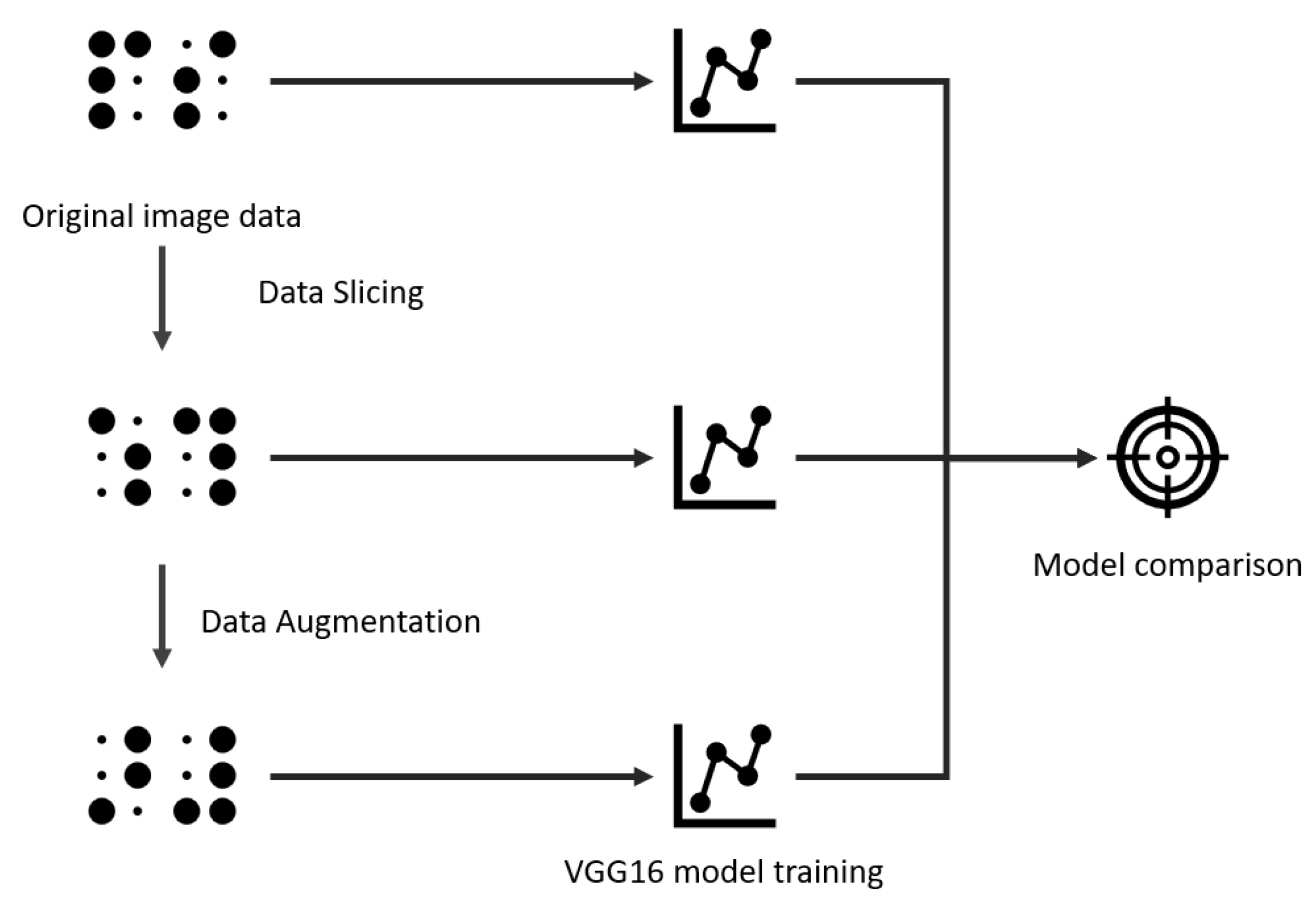
2. Methods and Materials

This section outlines the dataset, augmentation strategies, and the training and evaluation procedures used in this study. The methodology consists of taking the original dataset, performing the slicing and augmentation, and then training a VGG16 network (a deep convolutional neural network known for its simple architecture of stacked 3 × 3 convolutional layers and 16 weight layers, widely used for image classification tasks) [27] using three dataset versions: original, sliced, and augmented-sliced. The results were evaluated on a held-out test set, as illustrated in Figure 2.

Although VGG16 is an older CNN, it was selected for two reasons related to deployment in healthcare pipelines. First, it has modest resource requirements compared to modern CNNs. While alternatives like EfficientNet may offer similar or better performance [28,29], VGG16 serves as a suitable testbed to evaluate the benefits of augmentation. Second, VGG16 is well-supported and widely adopted in clinical applications, with a rich history of use and validation [30].

2.1. Dataset and Augmentation

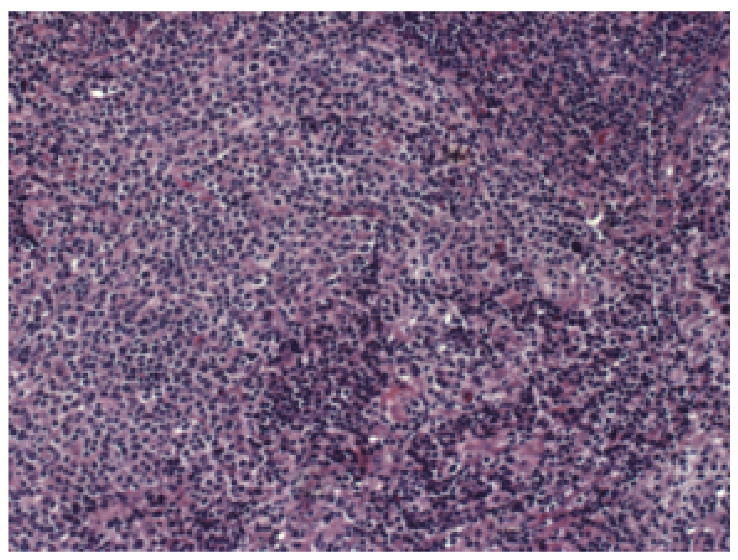
The dataset used in this study was the publicly available “Malignant Lymphoma Classification” [31], consisting of biopsy images stained with Hematoxylin/Eosin. The objective is to classify three malignant lymphoma types—chronic lymphocytic leukemia (CLL), follicular lymphoma (FL), and mantle cell lymphoma (MCL)—based solely on image data, avoiding probe-based diagnostics. All data images were captured using a Zeiss Axioscope microscope under white light illumination. The data acquisition employed a 20× objective and an AxioCam MR5 color CCD camera. Identical imaging parameters were maintained across all slides, including the same objective, camera, and light source, without normalization of camera channels [31]. The dataset is freely publicly available on Kaggle by its original authors (https://www.kaggle.com/datasets/andrewmvd/malignant-lymphoma-classification, accessed on 18 June 2025). Figure 3 provides an image example.

The dataset contains 374 TIF images at $1388\times 1040$ resolution: 113 CLL, 139 FL, and 122 MCL.

Augmentation

Two issues must be addressed before model training: the high image resolution and the limited sample size. Most CNNs require inputs of $224\times 224$ or $299\times 299$ [32], and resizing high-resolution images risks distorting crucial features or losing important diagnostic detail [33].

Second, the dataset’s small size (374 images) limits its utility for deep learning. When split into training, validation, and test subsets, each split contains too few samples, increasing the risk of overfitting.

To mitigate these challenges, a slicing strategy was applied: each $1388\times 1040$ image was divided into $224\times 224$ patches, forming a $6\times 4$ grid and expanding the dataset 24-fold. Figure 4 illustrates this process.

To further increase training data, deterministic augmentations were applied to each slice: rotations ($90\mathrm{deg}$, $180\mathrm{deg}$, $270\mathrm{deg}$), horizontal flip, and vertical flip. Figure 5a,b show an example patch and its augmented variants.

Augmentation increased the number of images uniformly across all classes, preserving balance.

Table 2. The number of images across classes in augmented datasets.

	CLL	FL	MCL
Original dataset	113	139	122
Sliced dataset	2712	3336	2928
Sliced and augmented dataset	16,272	20,016	17,568

summarizes image counts.

Each dataset variant was split into training, validation, and test subsets. The final evaluation used a test set unseen during training.

Table 3. The amount of images per class, in the original dataset and the augmented dataset.

	Total Images	Train	Validation	Test
Original dataset	374	239	60	75
Sliced dataset	8976	5744	1436	1796
Sliced and augmented dataset	53,856	34,467	8617	10,722

shows the distribution across subsets.

It may be pertinent to discuss trade-offs between score improvements and the computational cost of adding the slicing and augmentation step. While the slicing and augmentation are relatively simple computational tasks—especially if discussing applying it on a single image for inference, they are essentially negligible. The largest impact on the performance comes from the large increase in the amount of images used for training, as seen in Table 2. Still, this increase in computational time is kept to the training process which is completed once, prior to implementation, and it would not have significant impact during the exploitation of the developed models.

2.2. Classification Framework

Classification was performed using the VGG16 model [27], implemented in Keras. Training was conducted on a high-performance setup with five Nvidia Quadro RTX 6000 GPUs (24 GB each), dual Intel Xeon 6240R CPUs, and 768GB RAM.

VGG16’s moderate complexity enabled training on both high-resolution and augmented datasets without memory bottlenecks. Identical hyperparameters were used across all dataset variants: batch size of 8, maximum of 1000 epochs, and the Adam optimizer. An initial learning rate of 0.01 caused stagnation at 0.5, so it was reduced to $0.000001$, which resolved the issue.

To prevent overfitting, L2 regularization (0.01) was applied. Transfer learning was employed with weights pre-trained on ImageNet [34]. Categorical cross-entropy was used as the loss function.

Model Evaluation

Evaluation was based on the test set and included accuracy, AUC, precision, sensitivity, specificity, and F1 score. A one-vs-rest (OvR) scheme was used for the three-class problem, treating each class as positive in turn.

Binary classification metrics—false positives ($FP$), false negatives ($FN$), true positives ($TP$), and true negatives ($TN$)—were computed for each class. Metrics were then calculated as follows:

$$Accuracy={\displaystyle \frac{TP+TN}{TP+TN+FP+FN}}.$$

(1)

$$Precision={\displaystyle \frac{TP}{TP+FP}},$$

(2)

$$Sensitivity={\displaystyle \frac{TP}{TP+FN}}.$$

(3)

$$Specificity={\displaystyle \frac{TN}{TN+FP}}.$$

(4)

$$F1={\displaystyle \frac{2·Precision·Sensitivity}{Precision+Sensitivity}}.$$

(5)

All metrics range from 0 to 1, with 1 indicating perfect classification. Final results were obtained by averaging the metrics across all three classes.

3. Results

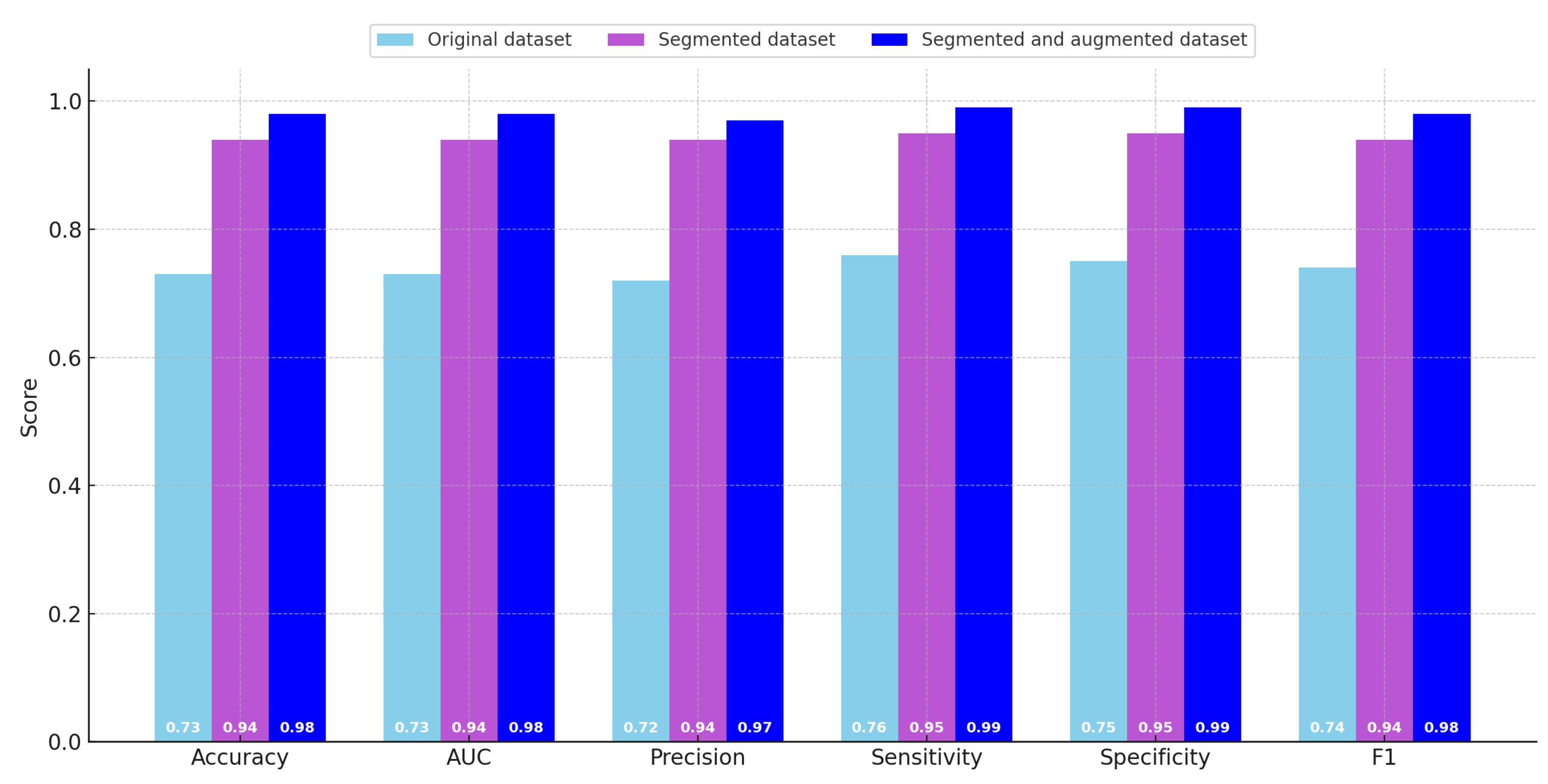
The principal results obtained through the evaluation of the trained classification models are presented in

Table 4. Achieved results across all datasets, for previously described metrics (higher value represents better classification performance).

	Accuracy	AUC	Precision	Sensitivity	Specificity	F1
Original dataset	0.733	0.729	0.718	0.757	0.750	0.737
Sliced dataset	0.943	0.943	0.940	0.946	0.947	0.943
Augmented dataset	0.978	0.978	0.970	0.986	0.986	0.978

, which summarizes the quantitative metrics across the different datasets, and are further illustrated graphically in Figure 6 to facilitate easier comparative visualization. As previously described in earlier sections, the evaluated metrics include classification accuracy, area under the curve (AUC), precision, sensitivity (also known as recall), specificity, and the F1 score. These metrics were computed in an averaged manner across the three classes included in the dataset.

Upon reviewing the metrics, a clear trend emerges: there was a consistent and substantial improvement in model performance when transitioning from the original dataset to the sliced dataset. The evaluation scores on the original dataset were generally low across most metrics. In particular, all metrics—except for sensitivity—fall within the range of 0.70 to 0.75, which is generally regarded as insufficient for reliable classification, especially when dealing with a dataset of limited size. Notably, the sensitivity score for the original dataset slightly exceeds 0.75, indicating that the model has a relatively better ability to identify true positive instances compared to its performance on other metrics.

With the introduction of the sliced dataset, there was a marked increase in performance across all evaluation measures. In this configuration, the model achieves an accuracy of 0.943, which represents a considerable improvement over the original dataset. Furthermore, both sensitivity and specificity reach high values of 0.946 and 0.947, respectively, while the lowest metric in this case (precision) is still high at 0.940. These results indicate that the model trained on the sliced dataset was significantly more robust and effective in distinguishing between the three classes.

The highest classification performance was obtained using the augmented dataset, which benefits from both the slicing and augmentation strategies previously described. In this scenario, the accuracy, AUC, and F1 score all achieve values of 0.978. The specificity and sensitivity metrics both reach a high of 0.986. While precision was slightly lower than the other metrics in this case, it still reaches a strong value of 0.970, making it the lowest among high-performing metrics. These results confirm the efficacy of data augmentation in enhancing the generalization and reliability of the trained models.

By examining the progression of scores, it becomes evident that the transition from the original dataset to the sliced dataset yields the most dramatic increase in classification performance. Although the performance gains between the sliced dataset and the augmented dataset were more modest in comparison, the use of the augmented dataset still enables the model to surpass a 0.95 threshold across all evaluated metrics. Despite these clear benefits in terms of performance, it was important to acknowledge that using the augmented dataset introduces a substantial increase in computational cost. Specifically, the training time required for the model to converge when using the augmented dataset was significantly higher than the time needed for training on either the original or sliced datasets.

To provide further insight into the improvement between the models trained on different datasets, the absolute differences in scores are summarized in

Table 5. The score difference between the data trained on “Model 1” and “Model 2” (higher value represents better classification performance).

Model 1	Model 2	$\mathbf{\Delta }$Accuracy	$\mathbf{\Delta }$AUC	$\mathbf{\Delta }$Precision	$\mathbf{\Delta }$Sensitivity	$\mathbf{\Delta }$Specificity	$\mathbf{\Delta }$F1	MIN	MAX	AVG
Original	Sliced	0.21	0.21	0.22	0.19	0.2	0.2	0.19	0.22	0.21
Sliced	Augmented	0.04	0.04	0.03	0.04	0.04	0.04	0.03	0.04	0.04
Original	Augmented	0.25	0.25	0.25	0.23	0.24	0.25	0.23	0.25	0.24

. This table compares each pair of dataset configurations in terms of how much improvement was observed across all six performance metrics. The final three columns present the minimum, maximum, and average score differences for each pairwise comparison.

From the values reported in Table 5, it can be concluded that the average performance improvement when moving from the original dataset to the sliced dataset was approximately 0.21 across the six metrics. In this comparison, the smallest improvement was observed in the specificity metric, with a value of $\mathsf{\Delta }Specificity=0.19$, while the largest improvement was observed in precision, which increases by $\mathsf{\Delta }Precision=0.22$. When evaluating the change in performance between the sliced dataset and the augmented dataset, the average increase across metrics was significantly smaller, amounting to 0.04. In this comparison, the precision shows the smallest increase at $\mathsf{\Delta }Precision=0.03$, with the other five metrics all exhibiting a consistent improvement of 0.04. When comparing the original dataset directly with the augmented dataset, the average performance gain was the largest, reaching a value of 0.24. In this case, specificity once again appears as one of the metrics contributing to this considerable gain.

Figure 7 shows the confusion matrices for the classification task using the original dataset, the sliced dataset, and the augmented dataset. The improvement in classification performance is clearly visible as the dataset size increases. In the original dataset, a notable amount of confusion is present between all classes. With slicing, the classification accuracy improves, reflected in higher true positive counts and fewer off-diagonal errors. The augmented dataset yields the best performance, with very few misclassifications, indicating that the augmentation strategy effectively enhances the model’s generalization ability.

A series of paired t-tests were conducted to assess whether the performance improvements across datasets (original, sliced, and augmented) were statistically significant. As shown in

Table 6. Paired t-test p-values for performance metric differences between datasets.

Comparison	Accuracy	AUC	Precision	Sensitivity	Specificity	F1
Original vs. sliced	0.0012	0.0011	0.0013	0.0010	0.0010	0.0012
Sliced vs. augmented	0.0215	0.0223	0.0287	0.0174	0.0180	0.0251
Original vs. augmented	0.0005	0.0006	0.0007	0.0004	0.0004	0.0006

, the differences in accuracy, AUC, precision, sensitivity, specificity, and F1 score were all statistically significant ($p<0.05$) when comparing the original dataset to both the sliced and augmented datasets. Additionally, improvements from the sliced to augmented dataset were also significant, though with slightly higher p-values, indicating smaller but still consistent performance gains. These results confirm that both the slicing and augmentation steps led to measurable and statistically significant improvements in classification performance.

4. Conclusions

In the presented paper, the authors have applied a slicing and augmentation procedure to the dataset. This dataset consists of 374 images split into three different classes of malignant lymphoma—MCL, CLL, and FL. After the slicing and augmentation were performed, the authors used a simple CNN—VGG16—to perform a multiclass classification between the three classes.

Using both slicing and augmentation shows an improvement in scores. Simply slicing the original images into smaller segments of the dimensions $224\times 224$ shows the average improvement of scores equal to 0.21. Adding augmentation into the pipeline achieves a further improvement of 0.04 (total 0.24 compared to simply training on the original dataset). This means that the highest scores were achieved with the combination of slicing and augmentation, with an F1 score of 0.98, specificity and sensitivity of 0.99, precision of 0.97, as well as AUC and accuracy of 0.98. These scores show the model being of satisfactory performance, with the model being able to differentiate between the three classes of malignant lymphoma with high accuracy.

Comparing to the state-of-the-art scores on this and similar datasets, as given in Table 1, it can be seen that the best scores achieved by the developed model were higher than the comparative studies. The scores on the original dataset were significantly lower, indicating that some processing or more advanced classification techniques—as used in the other reviewed research—were necessary to achieve satisfactory results. Additionally, it should be noted that the most significant improvement in scores came from slicing, and while these results were lower than the results achieved by the other reviewed research in Table 1, they are comparable. This indicates that similar or even better scores might be achievable simply using a more advanced classification network than VGG16, without the need for the application of augmentation, which significantly increases the data size and training times. The codes used in this paper are available as Github gists, with the image slicer and augmenter available at https://gist.github.com/ssegota/617bc81698de9a2b3ef62643e3d77024 (accessed on 18 June 2025), and the model trainer at: https://gist.github.com/ssegota/bb3a3a92c410c3e0185231a78b7abca8 (accessed on 18 June 2025).

Regarding the posed research questions (RQs), they can be addressed as follows:

• RQ1—the use of image slicing has a significant effect on the performance of the model compared to training on original data, increasing the scores on average by 0.21. This shows that the use of image slicing is a viable approach to increase the performance of the model in cases where the dataset consists of images that are significantly larger than the planned inputs for the CNN.
• RQ2—the use of simple geometric augmentation on sliced images does show an improvement when the scores are compared to the model trained on sliced images, although significantly smaller than the difference between the models trained on original and sliced images. This indicates that while geometric augmentation can improve scores, researchers should determine whether the additional computational cost is necessary, for a slight improvement. Since the performance was increased above 0.95 for all scores when using this technique in the presented research, it can be concluded that it is viable in some cases.
• RQ3—Multiclass classification of malignant lymphoma between MCL, FL, and CLL types can be performed with satisfactory scores (all metrics above 0.95), but processing techniques need to be applied to the images to achieve this. The use of image slicing and augmentation can be used to achieve this, but the use of more advanced classification networks might be able to achieve this without the need for augmentation.

There are two main limitations of this study. First, the CNN used for classification is relatively simple compared to some state-of-the-art techniques in image classification today, and better results could have been achieved using more advanced techniques such as vision transformers (ViT) [35], twin transformers [36], ConvNeXt [37], CoAtNet [38], or self-supervised models like BEiT [39] and DINOv2 [40], all of which represent state-of-the-art approaches that leverage either attention mechanisms, improved convolutional design, or large-scale pretraining to achieve significantly improved classification performance [41]. This issue was addressed because the authors wanted to test the possibility of using image slicing and augmentation on the dataset, with the goal of score improvement, instead of attempting to achieve a higher scoring classification and the results show that high classification performance is achievable even with a relatively simple CNN. The other limitation of the study was that the preprocessing techniques—slicing and augmentation—cannot be applied to every type of medical imagery. In the case of more localized tumors obtained with, e.g., CT scans, the use of slicing would not be possible as most of the image slices would not contain any significant data relating to tumor type. Simple geometric augmentation may be used, but depending on the disease in question, researchers should pay heed to whether the images can realistically be rotated or flipped without creating unrealistic images. The approach as described here would mostly focus on the images obtained with certain methods, such as histopathological images, in which the entire image represents cancerous tissue, and is orientation agnostic. Future work in this area should focus on testing the approach that was developed on different types of appropriate medical image datasets, to determine whether it is viable to apply it to different diseases. In addition to this, testing the performance of different techniques and how they benefit from adding a computationally simple augmentation is planned as well. One of the key issues that need to be addressed prior to focusing on the applicability of the suggested methodology is identifying other diseases where images collected are significantly larger than the CNNs are designed for, and that may benefit from the image slicing and augmentation techniques shown here. This would allow for more detailed conclusions relating to the applicability of the augmentation methodology provided in this paper to different diseases. As it currently stands, it is impossible to discuss whether the method would generalize well across different datasets, although significant improvements shown when applied provide a definite motivation for further testing.