Abstract
Portfolio optimisation is a crucial decision-making task. Traditionally static, this problem is more realistically addressed as dynamic, reflecting frequent trading within financial markets. The dynamic nature of the portfolio optimisation problem makes it susceptible to rapid market changes or financial contagions, which may cause drifts in historical data. While reinforcement learning (RL) offers a framework that allows for the formulation of portfolio optimisation as a dynamic problem, existing RL approaches lack the ability to adapt to rapid market changes, such as pandemics, and fail to capture the resulting concept drift. This study introduces a recurrent proximal policy optimisation (PPO) algorithm, leveraging recurrent neural networks (RNNs), specifically the long short-term memory network (LSTM) for pattern recognition. Initial results conclusively demonstrate the recurrent PPO’s efficacy in generating quality portfolios. However, its performance declined during the COVID-19 pandemic, highlighting susceptibility to rapid market changes. To address this, an incremental recurrent PPO is developed, leveraging incremental learning to adapt to concept drift triggered by the pandemic. This enhanced algorithm not only learns from ongoing market data but also consistently identifies optimal portfolios despite significant market volatility, offering a robust tool for real-time financial decision-making.
1. Introduction
Portfolio optimisation represents a decision-making framework for distributing capital across various financial assets to simultaneously maximise anticipated investment returns while minimising risk exposure. Conventional portfolio management techniques are categorised into four methodologies: follow-the-winner, follow-the-loser, pattern-matching, and meta-learning approaches, all of which depend substantially on sampled data or predetermined financial models [1]. These traditional methods depend on accurate market behaviour predictions, yet often struggle to adapt to the inherently noisy fluctuations of market prices.
Recurrent reinforcement learning (RRL) algorithms are reinforcement learning (RL) algorithms that employ recurrent neural networks (RNNs) as function approximators. One of the earliest studies on applying RL to optimise financial investments was conducted by [2]. Moody et al. considered a portfolio of two assets, one risky asset and one risk-free asset. The authors proposed an RRL algorithm based on real-time recurrent learning (RTRL) [2]. The research provided empirical evidence in support of using RL to obtain optimal portfolios. Thus, Moody et al. extended their work by employing Q-learning to find optimal portfolios and compared the performance with that of the RRL algorithm [3]. The findings indicated that the Q-learning algorithm exhibits greater sensitivity to the selected value function and demonstrates less stable performance compared with the RRL algorithm. Additionally, it was suggested that the differential Sharpe ratio—a metric quantifying risk-adjusted returns as excess return per unit of volatility—serves as a more favourable reward function than portfolio profit [3,4].
Recently, RL has been applied to this dynamic context, enhancing multistage stochastic optimisation—a key technique in sequential portfolio strategies. The absence of statistical presumptions makes the RL approaches simple and adaptable to form an online learning problem [5]. The goal of RL is to sequentially learn optimal decisions from historical market data. The dynamic nature of financial markets motivates the incorporation of pattern recognition networks, such as RNNs, for their memory capabilities and dynamic data adaptation [6]. Drift caused by financial contagions, such as pandemics, is effectively handled by using incremental learning with the windowing technique [7].
This study investigates optimal asset allocation strategies through the application of recurrent proximal policy optimisation (PPO) for portfolio optimisation in simulated environments. Given that financial markets represent a partially observable environment susceptible to concept drift, adaptive approaches are essential for maintaining performance during market volatility. The main contributions of the study include the use of incremental learning and LSTM to address the issue of concept drift in dynamic portfolio optimisation. The experimental results indicate that the proposed incremental PPO approach generates adaptive investment strategies that produce high-quality portfolios, albeit with slightly elevated risk compared with a standard recurrent PPO approach.
The rest of this paper is structured as follows: Section 2 reviews related work in portfolio optimisation and reinforcement learning approaches. Section 3 provides background on RL and portfolio optimisation. Section 4 presents the implementation and proposed methods in this study. Section 5 describes the experimental procedure and evaluation methodology. Section 6 presents and discusses the results of the proposed models. Section 7 concludes the paper and suggests potential future works.
2. Related Work
RRL algorithms are RL algorithms that employ RNNs as function approximators. One of the earliest studies on applying RL to optimise financial investments was conducted by [2]. Moody et al. considered a portfolio of two assets, one risky asset and one risk-free asset. The authors proposed an RRL algorithm based on real-time recurrent learning (RTRL) [2]. The research provided empirical evidence in support of using RL to obtain optimal portfolios. Thus, Moody et al. extended their work by employing Q-learning to find optimal portfolios and compared the performance with that of the RRL algorithm [3]. The findings indicated that the Q-learning algorithm exhibits greater sensitivity to the selected value function and demonstrates less stable performance compared with the RRL algorithm. Additionally, it was suggested that the differential Sharpe ratio serves as a more favourable reward function than portfolio profit [3,4]. The RRL strategy by Moody et al. gained popularity and it was explored by many researchers to search for optimal portfolios in different financial markets [8,9,10].
Jiang et al. proposed a deterministic policy gradient (DPG) algorithm [11], which utilised convolutional neural networks (CNNs) to predict the potential growth of the assets in the immediate future [1]. The algorithm used historical data that included the opening, highest, closing, and lowest (OHCL) prices of assets. The model was evaluated on the cryptocurrency exchange market data. The experiments showed that the framework achieved a higher Sharpe ratio and cumulative portfolio value when compared with other portfolio optimisation models. Shashank et al. evaluated the ability of deep deterministic policy gradient (DDPG) to construct risk aware portfolios [12]. The model effectively optimised the Sortino ratio [13] and found a portfolio with higher returns and lower variance [12]. Chaouki et al. investigated the ability of the DDPG algorithm to efficiently obtain optimal portfolios for constrained portfolio optimisation problems. The DDPG-based strategy was trained in a supervised manner where optimal policies were assumed to be known [14]. The performance showed that the proposed strategy converged to close-to-optimal portfolios.
More recently, Sood et al. conducted a comprehensive comparison between deep RL (DRL) and mean-variance optimisation for portfolio allocation using S&P500 sector indices [15]. Their PPO-based approach demonstrated superior performance over MVO across multiple metrics, including Sharpe ratio, maximum drawdown, and absolute returns. The study notably addressed a key limitation in the field by ensuring both methods were optimised for the same objective function and provided detailed implementation specifics for practical deployment. Recently, an anti-risk method for portfolio optimisation based on advantage actor critic (A2C) was proposed [16]. Yue et al. utilised supervised feature extraction techniques to approximate the true state of financial markets, and maximised the Sharpe ratio based on the output of a feature extractor [16].
3. Background
This section establishes the theoretical foundation for this study by reviewing key concepts for the proposed approach. Specifically, portfolio optimisation, RL, RNNs, including LSTM, and incremental learning are discussed in this section.
3.1. Portfolio Optimisation
Portfolio optimisation was first introduced through the mean-variance model by Markowitz [17]. The mean-variance model is a quadratic programming model used to determine a set of proportions that represents an optimal trade-off between the risk and returns [17]. It is formally defined as
where is the total risk of the portfolio, R is the total return on investment, and represents the preference value, also known as the risk tolerance. Optimal solutions are obtained by solving Equation (1) for varying values of . Portfolio return is maximised when . When , the portfolio risk is maximised. A trade-off between risk and return is attained when .
Risk is evaluated as
where n is the total number of assets in a portfolio, and and are proportions of the fund held in the assets i and j, respectively. The proportions are also referred to as portfolio weights. The covariance between assets i and j is denoted by . The expected return of a portfolio is calculated as
where denotes the expected return of the asset i. The total budget of the portfolio must be distributed among all the available assets. Thus, when the budget constraint is imposed, and Equations (2) and (3) are substituted in Equation (1), the mean-variance model is expressed as
3.2. Reinforcement Learning
RL is an effective and theoretically grounded area of machine learning inspired by behaviourist psychology [19]. It is a sub-field of machine learning, along with supervised and unsupervised learning. RL is defined as a computational approach carried out to understand and automate goal-directed learning, based on the science of decision making. In its standard form, RL allows solving single-objective optimisation problems which are usually modelled as Markov decision processes (MDPs) [20].
An MDP is an environment where all states are Markovian. Formally, an MDP is defined as a tuple , where is the state space of a finite set of states, is the action space of a finite set of actions, is the transition function, , that specifies the probability of arriving at after taking action a in state s. The reward function, , where , specifies the expected immediate reward associated with transitioning from state s to state , through action a. The variable is a discount factor with . MDPs possess the Markov property that the transition to state only depends on the last previously visited state and forgets about the other prior visited states.
3.3. Recurrent Neural Networks
RNNs are stateful sequential models that can be used to address the partial observability property of sequential decision making problems. RNNs [6] are feed-forward neural networks (ANNs) with feedback connections. The outputs of the model are fed back into itself and form a loop. The way RNNs are designed provides the ability to process a sequence of values using the parameter sharing approach [21]. RNNs model dynamical systems of the following state relations:
where is a state of the system at time step t and parameterise the function . The function maps the previous state to the next state . The sequence of historical data points, , is represented by .
The standard RNN with T inputs has a corresponding output vector of the same size T. The objective of the RNN model is to solve an optimisation problem defined as
where can be a regression or a classification loss function such as mean squared error [22] or negative log-likelihood [22]. The parameter is a vector of weights that parameterise the network. The optimisation problem is solved by applying gradient-based optimisation techniques. RNNs are trained with the back-propagation through time (BPTT) algorithm [23]. BPTT is a backpropagation algorithm that efficiently calculates the contribution of each network parameter to the loss function across all time steps.
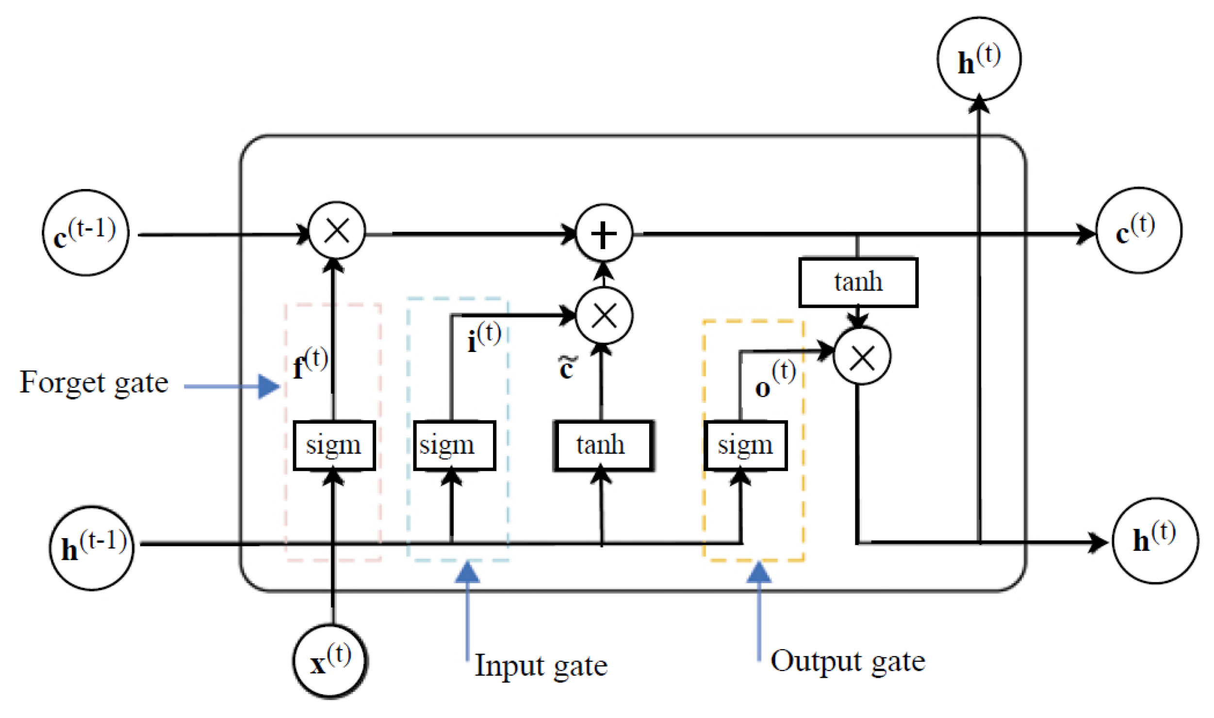
In practice, RNNs tend to suffer from exploding or vanishing gradients [24]. Vanishing gradients hinder optimisation of the loss function, while exploding gradients result in an unstable learning process of the model. Variants of RNNs, such as LSTMs [25], overcome these error back-flow problems. LSTMs are RNNs with internal recurrences that produce paths where the gradients can flow for a longer duration [21]. Figure 1 illustrates the structure of an LSTM cell.

Figure 1.
An illustration of an LSTM cell.
The gates in the LSTM cell serve different purposes. The weights associated with the self-loop are controlled by a forget gate responsible for filtering out old information at every timestep t. The cell state determines which information to store for future processing. Thus, hidden states are non-linearly shaped and do not accumulate information from the history of past observations.
3.4. Incremental Learning
Incremental learning is an active learning technique used to train ANNs to perform specific tasks. Normally, ANNs are trained to learn a task using a set of data samples. Incremental learning trains ANNs on an initial subset of a training set called the candidate set [7]. During training, more subsets of the candidate set are added to the training data using a set criterion. The new subsets can be added after a certain number of episodes, or when the model is no longer learning and the accuracy is no longer improving [7]. The process is repeated until the training data contains all subsets of the candidate set. The model trains on the training data as it increases and the candidate set decreases. The subsets of the candidate set are sampled without replacement using an active learning operator defined in [7] as
where , and are sets such that and is a vector of parameters of the neural network. The operator performs calculations on elements of to determine whether they should be added to the subset . The incremental learning process is illustrated in Algorithm 1 [7].
| Algorithm 1: Incremental Learning |
|
4. Proposed Methods
This section presents the proposed methods utilised for the portfolio optimisation in this study. Specifically, the design of the simulation environment, the proposed PPO algorithms, and the implementation specifics are addressed in this section.
4.1. Simulation Environment
OpenAI Gym: A simulation environment is an essential part of the RL system. It determines how the agent observes the environment and evaluates actions taken by the agent. The environment specifies the goal of an agent with a reward function and so prescribes the desired behaviour of an agent. An environment for the portfolio optimisation problem is simulated in Gym (https://github.com/openai/gym accessed on 21 May 2023). Gym is an open-source RL toolkit developed by OpenAI with a wide range of simulation environments. Amongst the numerous environments, Gym also allows third-party environments to be created by inheriting a defined standard class.
Assumptions: RL agents apply back-test trading to learn optimal investment strategies from observing the changes in historical prices of financial assets. Back-test trading is whereby a trading agent pretends to be back in time at a point in the financial market history and paper trades from then onward, without any knowledge of future market information. Paper trading is learning how to optimally buy, sell, or hold assets in a simulated environment using fake capital. The following assumptions are imposed in order to simulate a financial market environment appropriate for RL trading agents [1]:
- There exists sufficient market liquidity and zero slippage. That is, all assets are liquid, and each trade can be finished immediately at the price at which an order is placed.
- There is no impact on the market. That is, the capital invested by the RL algorithm is insignificant and has no influence on the market.
State Space: The state space is characterised as a combination of historical asset prices and returns. Given the impossibility of capturing a complete state space from the unknown high-dimensional characteristics of financial markets, the state is approximated through observable samples to streamline the state-space representation. Financial markets are partially observable environments. At any time step t, the agent can only observe absolute asset prices, which do not give information about the dynamics of financial markets. Asset returns give the rate of change of asset prices. However, logarithmic returns or log returns are statistically superior to asset prices and simple returns when predicting financial markets. The observation of log returns enables the cross-asset dependencies to be captured because the summation of log returns equivalently leads to the multiplication of gross returns. The products of gross returns are building factors when covariances between assets are computed. Therefore, the observation space is represented by the log returns of assets, given as
where is the logarithmic return of asset i at timestep t. However, one-period logarithmic returns cannot capture the complete state of the financial market.
Consequently, a log returns matrix, , of a shifting window of size T is used. The observation matrix is redefined as
The agent must use the observation to infer the underlying state of the environment and to construct an approximation of the actual environment state using an LSTM network. LSTMs are less computationally expensive as compared to complete history, since LSTMs are able to efficiently process historic observations in an adaptive manner, store information over a long timespan, and forget information that is no longer useful. The representative state of the environment is then defined as
where represents an LSTM layer which is a part of the policy network and thus, is a policy parameter.
Action Space: The action space for the portfolio optimisation problem is defined as the trading decision of an agent to reallocate each proportion of assets in the portfolio. At every timestep t, the RL agent must select a portfolio vector associated with N assets. In order to determine the portfolio vector, the agent must observe the environment state and take actions at every time step t, which, in turn, correspond to the portfolio vector at that time step . That is,
whereby the actions are scaled so that the proportions of the portfolio satisfy the budget constraint in Equation (5). That is,
and since short selling is prohibited in long-term portfolio management.
Reward Generating Function: Barto and Sutton [19] stated that the goal of an RL agent is described in terms of the reward signal. A reward signal is a scalar value that an agent receives at every time step. The agent aims to find a strategy that maximises the sum of received reward signals over time. The determination of an optimal reward-generating function is a known challenge in RL problems. In the case of portfolio optimisation problems, there are two objective functions, namely return and risk, which must be optimised simultaneously. A commonly investigated reward-generating function for RL-based portfolio optimisation is the Sharpe ratio.
When the Sharpe ratio is the reward-generating function, then both the portfolio return and risk are taken into account. The Sharpe ratio is a measure of risk-adjusted return. Therefore, the agent solves the portfolio problem,
4.2. Proximal Policy Optimisation
Amongst variants of the policy gradient method, PPO was implemented, which is said to have good stability during training of the algorithm [26]. PPO improves the training stability of the policy by constraining the change in the policy at each training epoch. Too large policy updates are avoided to prevent possible unrecoverable bad policies, while smaller updates are typically more likely to converge to an optimal solution. Unlike vanilla policy gradient methods, which aim to maximise the long-term returns over time, PPO maximises the generalised advantage estimation (GAE), , defined as
where
and is the approximated state value function; is the reward. The policy parameters are adjusted by an update rule, given as
where represents an action a selected following a parametrised policy . The function is a clipped objective function maximised through taking multiple steps of mini-batch stochastic gradient descent (SGD); is defined as
where is a hyperparameter set to bound how far away a new policy can be from the old policy ; and are parameters of new and old policies, respectively. Clipping ensures that a new policy is always bounded. That is, the ratio of the current policy to the previous policy falls in the range . The notion of clipping policies guarantees reasonable policy updates [27].
4.3. Implementation
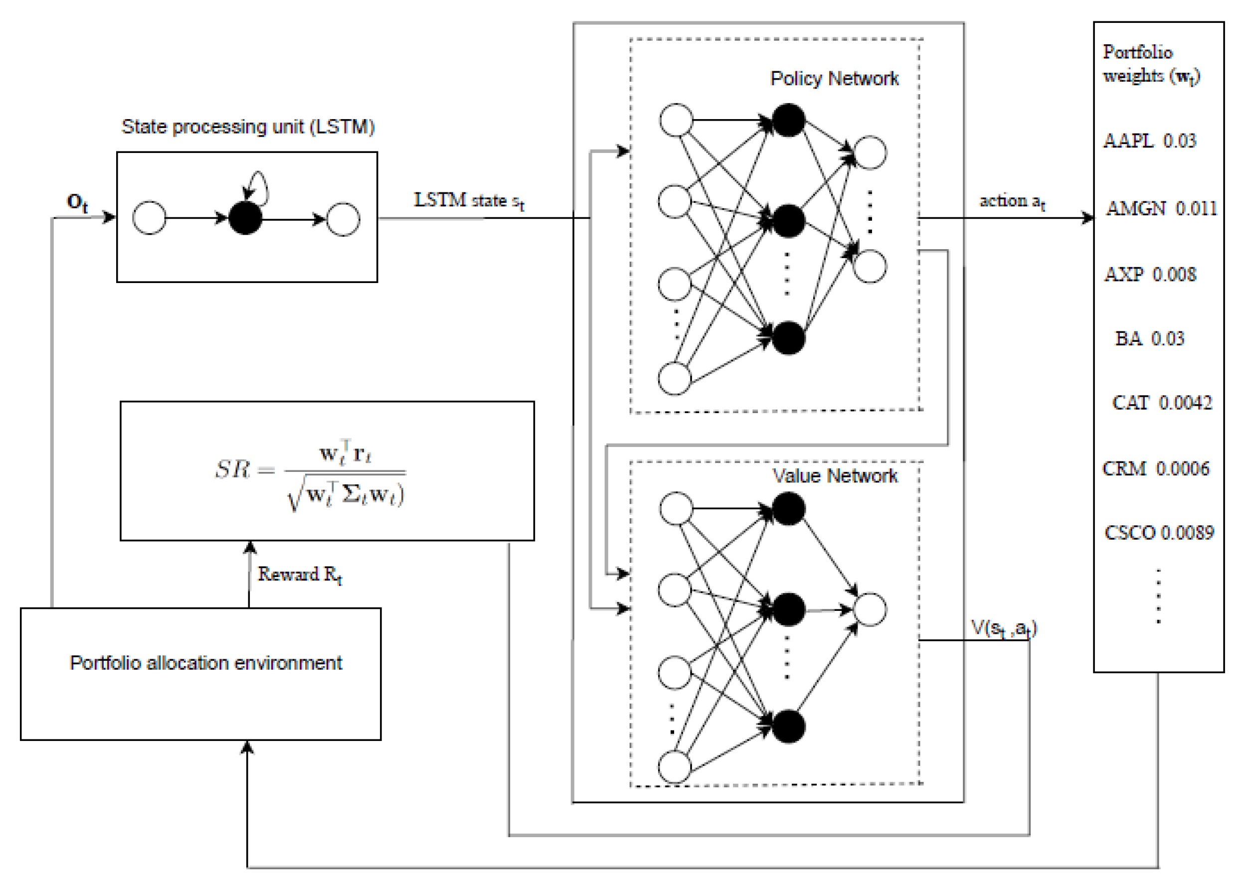
In RL algorithms, a policy that maps states to actions is represented by neural networks. The adopted recurrent PPO agent integrates two ANNs into a unified actor-critic network. The first ANN represents a policy network responsible for the policy function approximation. The policy function produces a probability distribution of portfolio weights. The second ANN, called a value network, predicts the value of the selected portfolio weights at each timestep. A timestep is defined as every open trading day in a trading period. Both networks share a single layer of an LSTM network. At each timestep, the agent receives a matrix of observations given by Equation (12). Each row i of the matrix represents a time series of log returns of an asset i. The observations are passed as input to the LSTM layer. The LSTM network processes the observations into an LSTM state used as a representation of the environment state. The LSTM state is transferred to the fully connected policy and actor networks. The policy network produces a probability distribution of actions that are sampled into portfolio weights. The value network estimates the value function, which is then used with the reward to calculate the GAE. The process is repeated for every timestep over multiple episodes. An episode is defined as the total number of timesteps in a trading period. If a trading period is 3 years, then an episode is equal to 756 timesteps. Figure 2 illustrates a schematic architecture of the proposed recurrent PPO model motivated by the work in [28].
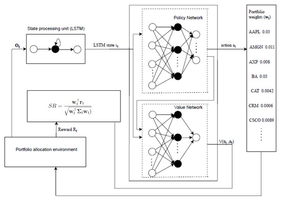
Figure 2.
A schematic illustration of a recurrent PPO model for portfolio optimisation.
Policy Optimisation: The goal of the agent is to find a policy that maximises the reward function given by Equation (16). The agent is trained to optimise a stochastic policy using collected experience. At the initial timestep, i.e., the first day of trading, the agent chooses an action using a random policy. A trajectory of states, actions, and rewards is added to a local storage called the replay buffer. This trajectory is referred to as the experience of an agent. The experience is added to the replay buffer asynchronously using the first-in-first-out (FIFO) method. When the replay buffer reaches a maximum capacity, old experiences are filtered out as new experience is added. The model gradients are computed using mini-batches of 504 timesteps of experience sampled from the replay buffer. The aim is to ensure that the agent uses very recent parameters to generate experience. The agent employs the adaptive moment estimation (Adam) optimiser [29] to update the policy network parameters, while the value network parameters are updated using SGD. The agent is trained until it achieves a deterministic stationary policy.
Training: RL agents are prone to lack of generalisation [30]. Hence, the early stopping technique was adopted to increase generalisation and to avoid model overfitting. The point at which to stop training was determined from a callback function that handled the validation of the policy. After every 10 episodes, the deterministic policy is validated and the model is saved if and only if the policy resulted in the highest average episode return compared with the previously evaluated policy. When the training terminates, the model with the best validation results is evaluated in the test environment. Here, the agent makes predictions using the deterministic policy. Normally, RL agents are tested in the same environment they have trained on [30]. However, for the portfolio optimisation problem, it is important to test the generalisation ability of the policy. Therefore, the agent was evaluated in a new market environment.
Training with Incremental Learning: The test dataset encompassed the full duration of the COVID-19 pandemic outbreak. This approach aimed to evaluate the recurrent PPO’s capacity to adjust to shifts in the environment’s underlying distribution caused by the pandemic. As the testing progressed, the recurrent PPO agent became obsolete over the trading period. In an attempt to improve the performance of recurrent PPO, incremental learning was introduced in model training. The training environment was cut down to an initial size equal to three years of training data. The size of the environment was systematically increased with a step size of six months of data as the agent continued to train. The agent was trained until the environment was complete, i.e., when the size of the observation space reached eight years of historical data. The goal was to allow the agent to incrementally learn the market and to allocate portfolios based on every old and new experience it has gathered. The trained model was tested on the entire four years of test data without increment. The reason for testing in a complete environment was to prohibit the agent from attempting to retrain if the test environment was incremented. Therefore, the incremental agent was tested in the same test environment as the recurrent agent.
5. Empirical Process
This section describes the empirical process used to evaluate the proposed methodology, including a description of the dataset, benchmark algorithms, control parameters of the proposed models, and performance measures employed in the experimental evaluation.
5.1. Data Description
The proposed strategy was trained over historical price data of 30 constituents listed on two American stock exchanges, namely the New York Stock Exchange (NYSE) and NASDAQ. All the data used were downloaded from the Yahoo Finance (https://finance.yahoo.com/ accessed on 23 May 2023) application programming interface. The data are a set of 94,888 samples and 9 features, which include open, high, low, and closing prices for each stock. The data dimensionality was reduced by considering the closing price as the only feature for the analysis. All the other features were dropped. Missing values were also dropped. Weekends were not considered open trading days. Therefore, there are 5 trading days in a week, 20 in a month, and 252 in a year. To allocate optimal portfolios, the agent must learn the market behaviour. Logarithmic returns of a fixed window of size 252 were used to represent environment observations at each timestep. The initial investment amount for all strategies during training and testing was . Table 1 shows the training and testing periods.

Table 1.
Trading periods considered for training and testing recurrent, and incremental PPO agents.
5.2. Benchmarks
The proposed strategy was compared with two benchmarks, namely the Dow Jones Industrial Average (DJIA) index and the sequential minimum variance model. DJIA is a price-weighted market index that measures the performance of stocks listed on the NYSE and NASDAQ. The sequential minimum variance model is the Markowitz mean-variance model with risk as its single objective, minimised with respect to return and boundary constraints. The model was derived by iteratively applying a one-step portfolio optimisation program solver, called PyPortfolioOpt [31], for each time step.
5.3. Control Parameters
The state processing unit is represented by a single layer of LSTMs with 64 hidden cells. The policy and value networks share the same parameters. The networks consist of two hidden layers of 128 neurons and the hyperbolic tangent activation function. The policy network output layer uses the softmax activation function since the result of the network is a probability distribution, which corresponds to portfolio weights. That is, each weight is a value in the range . The softmax function ensures that the boundary constraint is satisfied, i.e., the portfolio weights sum up to a unit. The activation function on the output layer of the value network is a linear function. The initialisation of actor-critic parameters was based on the parameters used to play Mujoco [32] and Atari [28], while the LSTM network parameters were selected by following the work conducted in [33]. The parameters were tuned using the random and grid search methods [34].
5.4. Performance Measures
The considered evaluation metrics are the cumulative returns (CR), which measure the accumulated portfolio return over the four years trading period as a percentage; average volatility (AV), which is the risk level of the portfolio at a given return level; maximum drawdown (MDD), which gives a measure of maximum loss percentage from a peak trough during the trading period; Sharpe ratio (SR), which measures the rate of return achieved per unit risk; the Calmar ratio (CMR), which measures the rate of return attained per unit MDD and value-at-risk (VAR), which measures the risk of loss from an investment given normal market conditions.
6. Results
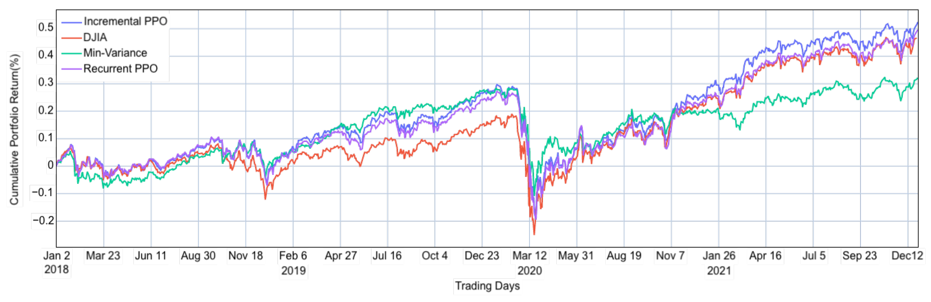
The experiment assessed the performance of both recurrent and incremental PPO agents in identifying optimal portfolios, comparing their performance against DJIA and a minimum variance model. Figure 3 depicts the daily portfolio allocations of the PPO models, DJIA, and the minimum variance model. The strong performance of the minimum variance model is justified, as it seeks to minimise the risk for any given level of return. Financial markets are inherently volatile, and unexpected events, such as the COVID-19 pandemic, exacerbate economic uncertainties and market volatility. Consequently, an investment strategy that prioritises volatility minimisation, like the minimum variance model, proves more advantageous during periods of high market turbulence.
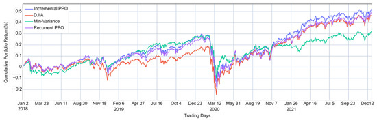
Figure 3.
Portfolio value on the Dow 30 stocks.
The recurrent PPO model consistently outperformed the market throughout the trading period and only surpassed the minimum variance model starting from November 2020 onward. According to the plot, it appears that the recurrent PPO model excels at identifying optimal portfolios under typical market conditions. The recurrent PPO agent employs an investment strategy developed through a backtesting approach, which relies on historical data reflective of standard market conditions. However, the model struggles to adjust to unexpected market shifts and tends to perform well only when the market conditions resemble those present during its training phase.
In contrast, the incremental PPO closely mirrored the performance of the minimum variance model from January 2019 through November 2020, demonstrating superior adaptability to market fluctuations. During the onset of the COVID-19 pandemic, all models experienced a downturn in performance. However, the incremental PPO demonstrated a robust recovery, with its cumulative returns quickly resuming an upward trajectory, while the recurrent PPO struggled to consistently outperform the DJIA. Unlike the recurrent PPO, which remained relatively static in its strategy, the incremental PPO adapted dynamically to market changes, optimising its portfolios effectively. Over the entire trading period, the incremental PPO consistently surpassed the performance of the other three models.
Table 2 presents the performance metrics across all four strategies. Among these approaches, incremental PPO achieved the highest performance with a CR of , SR of , and CMR of , and surpasses the other methodologies. Regarding risk assessment, the minimum variance model demonstrated superior performance compared with incremental PPO. The incremental PPO portfolios exhibited elevated risk levels relative to their recurrent PPO counterparts. A possible reason behind this is that incremental learning increases volatility in the simulation environment by continuously increasing the training observation space. Therefore, the incremental PPO agent is robust and more risk-tolerant because it was trained in a more volatile environment than recurrent PPO. It is important to note that the market index, DJIA, found the most risky portfolios.
Table 2.
Results of incremental PPO strategy against recurrent PPO and the benchmark strategies.
Portfolios Analysis
The initial investment for each strategy was set at , with the assumption of no transaction costs. Over the four-year trading period, portfolios were adjusted daily. Both the recurrent and incremental PPO agents commenced trading with equal weights assigned to each stock on the first trading day. These weights were dynamically adjusted over time based on the strategies learned during their training phases. Throughout the trading period, both strategies demonstrated a preference for assets with historically higher returns, including all available assets in their portfolios. Despite these similarities, the outcomes varied significantly between the two approaches. The recurrent PPO faced substantial losses in 2020, persisting in its strategy of favouring historically high-return assets even as their prices continued to decline. Consequently, the strategy became less effective over time. In contrast, the incremental PPO adapted more effectively to market changes. Particularly during the dramatic shifts brought about by the COVID-19 pandemic, the incremental PPO adjusted by decreasing the weights of previously highly valued stocks. It transitioned to a more balanced approach, assigning nearly equal weights across all stocks and gradually adjusting priorities based on the most recent price changes.
While some portfolios managed under both strategies still incurred losses, the incremental PPO’s approach proved to be more dynamic and successful. It consistently adapted to the evolving market conditions, displaying a superior ability to mitigate risks and capture opportunities, in contrast to the more static strategy of the recurrent PPO.
7. Conclusions
The study presented in this paper assessed the efficacy of an incrementally trained recurrent proximal policy optimisation (PPO) agent in tackling the portfolio optimisation problem within a simulated financial market. PPO, a policy-based reinforcement learning algorithm, utilises dual neural networks to estimate policy functions and evaluate actions. A long short-term memory (LSTM) network was employed to decode the financial state from historical asset prices over a 252-day window, ensuring a focus on the most recent and relevant information.
The recurrent PPO algorithm was benchmarked against conventional portfolio strategies and demonstrated its ability to identify optimal portfolios. However, the inherent volatility and susceptibility to drifts in financial markets, often triggered by factors like economic news, social media influences, or global pandemics, adversely impacted its performance. Notably, the COVID-19 outbreak significantly undermined the recurrent PPO’s effectiveness. In response, the algorithm was incrementally trained to better adapt to sudden market changes. This adaptive approach allowed the incremental PPO to consistently generate superior portfolios, outperforming not only the standard PPO but also the minimum variance model and the DJIA index by a considerable margin.
Limitations and future work. Despite the improved performance of the incremental PPO, its susceptibility to significant market upheavals highlights a limitation in its current training regime. Future work will focus on enhancing the generalisation of reinforcement learning (RL) for portfolio optimisation across more diverse market conditions. Employing transfer learning is anticipated to significantly improve the sample efficiency of RL agents, potentially revolutionising how portfolio management is approached in dynamically changing environments. The proposed incremental recurrent RL approach was evaluated on a limited number of assets and compared with the DJIA and the mean-variance model as classical approaches used in portfolio optimisation. In addition, it was also compared with a non-incremental recurrent RL approach to show the benefit of incremental learning to a recurrent RL implementation. Future work will include wider comparisons with alternative approaches to portfolio optimisation.
Author Contributions
Conceptualisation, R.S. and A.E.; methodology, R.S. and A.E.; software, R.S.; validation, R.S.; formal analysis, R.S.; investigation, R.S. and A.E.; resources, R.S.; data curation, R.S.; writing—original draft preparation, R.S.; writing—review and editing, A.E. and K.A.; visualisation, R.S.; supervision, A.E.; project administration, R.S., A.E. and K.A. All authors have read and agreed to the published version of the manuscript.
Funding
This research received no external funding.
Institutional Review Board Statement
Not applicable.
Informed Consent Statement
Not applicable.
Data Availability Statement
The datasets generated during and/or analysed during the current study are available from the corresponding author upon reasonable request.
Conflicts of Interest
The authors declare no conflicts of interest.
References
- Jiang, Z.; Liang, J. Cryptocurrency portfolio management with deep reinforcement learning. In Proceedings of the IEEE Intelligent Systems Conference, Glasgow, UK, 21–23 August 2017; pp. 905–913. [Google Scholar]
- Moody, J.; Wu, L.; Liao, Y.; Saffell, M. Performance functions and reinforcement learning for trading systems and portfolios. J. Forecast. 1998, 17, 441–470. [Google Scholar] [CrossRef]
- Moody, J.; Saffell, M. Reinforcement Learning for Trading Systems and Portfolios. In Proceedings of the Knowledge Discovery and Data Mining, Montreal, QC, Canada, 27–31 August 1998; pp. 279–283. [Google Scholar]
- Moody, J.; Saffell, M. Learning to trade via direct reinforcement. IEEE Trans. Neural Netw. 2001, 12, 875–889. [Google Scholar] [CrossRef] [PubMed]
- Agarwal, A.; Hazan, E.; Kale, S.; Schapire, R.E. Algorithms for portfolio management based on the newton method. In Proceedings of the International Conference on Machine Learning, Pittsburgh, PA, USA, 25–29 June 2006; pp. 9–16. [Google Scholar]
- Rumelhart, D.E.; Hinton, G.E.; Williams, R.J. Learning representations by back-propagating errors. Nature 1986, 323, 533–536. [Google Scholar] [CrossRef]
- Engelbrecht, A.P. Computational Intelligence: An Introduction; John Wiley & Sons: Hoboken, NJ, USA, 2007. [Google Scholar]
- Gabrielsson, P.; Johansson, U. High-frequency equity index futures trading using recurrent reinforcement learning with candlesticks. In Proceedings of the IEEE Symposium Series on Computational Intelligence, Singapore, 8–10 December 2015; pp. 734–741. [Google Scholar]
- Zhang, J.; Maringer, D. Indicator selection for daily equity trading with recurrent reinforcement learning. In Proceedings of the Genetic and Evolutionary Computation Conference Companion, Amsterdam, The Netherlands, 6–10 July 2013; pp. 1757–1758. [Google Scholar]
- Zhang, J.; Maringer, D. Two parameter update schemes for recurrent reinforcement learning. In Proceedings of the IEEE Congress on Evolutionary Computation, Beijing, China, 6–11 July 2014; pp. 1449–1453. [Google Scholar]
- Silver, D.; Lever, G.; Heess, N.; Degris, T.; Wierstra, D.; Riedmiller, M. Deterministic policy gradient algorithms. In Proceedings of the International Conference on Machine Learning, Beijing, China, 21–26 June 2014; pp. 387–395. [Google Scholar]
- Hegde, S.; Kumar, V.; Singh, A. Risk aware portfolio construction using deep deterministic policy gradients. In Proceedings of the IEEE Symposium Series on Computational Intelligence, Rio de Janeiro, Brazil, 6–8 November 2018; pp. 1861–1867. [Google Scholar]
- Sortino, F.A.; Van Der Meer, R. Downside risk. J. Portf. Manag. 1991, 17, 27. [Google Scholar] [CrossRef]
- Chaouki, A.; Hardiman, S.; Schmidt, C.; Sérié, E.; De Lataillade, J. Deep deterministic portfolio optimization. J. Financ. Data Sci. 2020, 6, 16–30. [Google Scholar] [CrossRef]
- Sood, S.; Papasotiriou, K.; Vaiciulis, M.; Balch, T. Deep reinforcement learning for optimal portfolio allocation: A comparative study with mean-variance optimization. Plan. Sched. Financ. Serv. 2023, 2023, 21. [Google Scholar]
- Yue, H.; Liu, J.; Tian, D.; Zhang, Q. A Novel Anti-Risk Method for Portfolio Trading Using Deep Reinforcement Learning. Electronics 2022, 11, 1506. [Google Scholar] [CrossRef]
- Markowitz, H. Portfolio Selection. J. Financ. 1952, 7, 77–91. [Google Scholar]
- Sharpe, W.F. Capital asset prices: A theory of market equilibrium under conditions of risk. J. Financ. 1964, 19, 425–442. [Google Scholar]
- Sutton, R.S.; Barto, A.G. Reinforcement Learning: An Introduction; MIT Press: Cambridge, MA, USA, 2018. [Google Scholar]
- Bellman, R. A Markovian decision process. J. Math. Mech. 1957, 6, 679–684. [Google Scholar] [CrossRef]
- Goodfellow, I.; Bengio, Y.; Courville, A. Deep Learning; MIT Press: Cambridge, MA, USA, 2016. [Google Scholar]
- Wang, Q.; Ma, Y.; Zhao, K.; Tian, Y.J. A Comprehensive Survey of Loss Functions in Machine Learning. Ann. Data Sci. 2022, 9, 187–212. [Google Scholar] [CrossRef]
- Werbos, P.J. Backpropagation Through Time: What It Does and How to Do It. Proc. IEEE 1990, 78, 1550–1560. [Google Scholar] [CrossRef]
- Pascanu, R.; Mikolov, T.; Bengio, Y. On the difficulty of training recurrent neural networks. In Proceedings of the International Conference on Machine Learning, Atlanta, GA, USA, 16–21 June 2013; pp. 1310–1318. [Google Scholar]
- Hochreiter, S.; Schmidhuber, J. Long Short-Term Memory. Neural Comput. 1997, 9, 1735–1780. [Google Scholar] [CrossRef] [PubMed]
- Luo, P.; Xiong, H.Q.; Zhang, B.; Peng, J.; Xiong, Z.F. Multi-resource constrained dynamic workshop scheduling based on proximal policy optimisation. Int. J. Prod. Res. 2022, 60, 5937–5955. [Google Scholar] [CrossRef]
- Schulman, J.; Wolski, F.; Dhariwal, P.; Radford, A.; Klimov, O. Proximal Policy Optimization Algorithms. arXiv 2017, arXiv:1707.06347. [Google Scholar]
- Huang, S.; Dossa, R.F.J.; Raffin, A.; Kanervisto, A.; Wang, W. The 37 Implementation Details of Proximal Policy Optimization. In Proceedings of the International Conference on Learning Representations Blog Track, Virtually, 25–29 April 2022. [Google Scholar]
- Kingma, D.P.; Ba, J. Adam: A method for stochastic optimization. arXiv 2014, arXiv:1412.6980. [Google Scholar]
- Cobbe, K.; Klimov, O.; Hesse, C.; Kim, T.; Schulman, J. Quantifying generalization in reinforcement learning. In Proceedings of the International Conference on Machine Learning, Long Beach, CA, USA, 9–15 June 2019; pp. 1282–1289. [Google Scholar]
- Martin, R.A. PyPortfolioOpt: Portfolio optimization in Python. J. Open Source Softw. 2021, 6, 3066. [Google Scholar] [CrossRef]
- Todorov, E.; Erez, T.; Tassa, Y. MuJoCo: A physics engine for model-based control. In Proceedings of the IEEE/RSJ International Conference on Intelligent Robots and Systems, Lisbon, Portugal, 7–12 October 2012; pp. 5026–5033. [Google Scholar]
- Yu, P.; Yan, X. Stock price prediction based on deep neural networks. Neural Comput. Appl. 2020, 32, 1609–1628. [Google Scholar] [CrossRef]
- Bergstra, J.; Bengio, Y. Random search for hyper-parameter optimization. J. Mach. Learn. Res. 2012, 13, 281–305. [Google Scholar]
Disclaimer/Publisher’s Note: The statements, opinions and data contained in all publications are solely those of the individual author(s) and contributor(s) and not of MDPI and/or the editor(s). MDPI and/or the editor(s) disclaim responsibility for any injury to people or property resulting from any ideas, methods, instructions or products referred to in the content. |
© 2025 by the authors. Licensee MDPI, Basel, Switzerland. This article is an open access article distributed under the terms and conditions of the Creative Commons Attribution (CC BY) license (https://creativecommons.org/licenses/by/4.0/).