Review of Deep Learning Applications for Detecting Special Components in Agricultural Products

Abstract

The rapid evolution of deep learning (DL) has fundamentally transformed the paradigm for detecting special components in agricultural products, addressing critical challenges in food safety, quality control, and precision agriculture. This comprehensive review systematically analyzes many seminal studies to evaluate cutting-edge DL applications across three core domains: contaminant surveillance (heavy metals, pesticides, and mycotoxins), nutritional component quantification (soluble solids, polyphenols, and pigments), and structural/biomarker assessment (disease symptoms, gel properties, and physiological traits). Emerging hybrid architectures—including attention-enhanced convolutional neural networks (CNNs) for lesion localization, wavelet-coupled autoencoders for spectral denoising, and multi-task learning frameworks for joint parameter prediction—demonstrate unprecedented accuracy in decoding complex agricultural matrices. Particularly noteworthy are sensor fusion strategies integrating hyperspectral imaging (HSI), Raman spectroscopy, and microwave detection with deep feature extraction, achieving industrial-grade performance ($RPD$ > 3.0) while reducing detection time by 30–100× versus conventional methods. Nevertheless, persistent barriers in the “black-box” nature of complex models, severe lack of standardized data and protocols, computational inefficiency, and poor field robustness hinder the reliable deployment and adoption of DL for detecting special components in agricultural products. This review provides an essential foundation and roadmap for future research to bridge the gap between laboratory DL models and their effective, trusted application in real-world agricultural settings.

1. Introduction

Special components in agricultural products encompass a diverse array of chemical, biological, and physical constituents that critically influence product safety, quality, and physiological integrity. These components are distinguished by their significant impact on human health, market value, and agricultural sustainability, yet they often occur at trace levels or exhibit complex interactions within biological matrices, rendering their detection analytically challenging. Broadly categorized, special components include (1) safety-critical hazards such as pesticide residues (e.g., chlorpyrifos in oils [1]), heavy metals (e.g., cadmium in lettuce [2], lead in oilseed rape [3,4]), mycotoxins (e.g., aflatoxin B₁ in maize [5]), and polycyclic aromatic hydrocarbons [6] (e.g., benzofluoranthene in seafood), which pose direct risks to consumers; (2) quality-defining attributes like soluble solids content in fruits [7], tea polyphenols [8], starch functional properties [9], gel strength in processed foods [10], and texture parameters (e.g., resilience in tofu [11]), which determine sensory acceptability and economic value; and (3) physiological markers, including chlorophyll (Chl) content [12], anthocyanin levels [13], moisture dynamics [14], and nutrient status (e.g., nitrogen in crops), which reflect plant health, stress responses, and post-harvest physiological changes.

The inherent complexity of agricultural systems, characterized by heterogeneous matrices, environmental variability, and dynamic biological processes, imposes stringent demands on detection methodologies. Traditional methods for detecting special components in agricultural products face significant constraints that impede efficient quality and safety monitoring, including chromatography (e.g., high-pressure liquid chromatography [15], gas chromatography–mass spectrometry) [16,17,18,19,20], atomic spectroscopy (e.g., inductively coupled plasma mass spectrometry (ICP-MS) [21,22]), and immunoassays [23,24,25,26]. These techniques are inherently destructive, requiring extensive sample preparation and chemical reagents, which prolongs the analysis time (often hours per sample) and increases operational costs. Moreover, their reliance on laboratory infrastructure and skilled personnel limits the field deployment, hindering real-time decision making in agricultural supply chains. For spectral-based methods such as near-infrared (NIR) or HSI [27,28,29], challenges persist in handling high-dimensional data with noise interference, baseline drift, and redundant variables, which degrade model robustness and generalizability across various crop matrices. Consequently, the precise identification and quantification of these special components require innovative approaches that transcend conventional analytical paradigms.

Deep learning (DL) techniques address these limitations by automating feature extraction and enabling end-to-end modeling [6,14,30,31,32,33]. Convolutional neural networks (CNNs) transform raw spectral data into discriminative spatial features, bypassing manual preprocessing steps like Savitzky–Golay smoothing or multiplicative scatter correction [34,35]. Recurrent architectures (e.g., long short-term memory (LSTM) networks [36]) capture temporal dependencies in sequential spectral data, enhancing prediction stability for dynamic processes such as fermentation or drying. Attention mechanisms [37] (e.g., Squeeze-and-excitation networks (SENet) [38,39], residual attention modules) further refine feature selection by adaptively weighting informative wavelengths or channels, mitigating interference from complex backgrounds. These capabilities allow DL models to achieve state-of-the-art accuracy in quantifying trace contaminants (e.g., aflatoxins at 0.03 mg/kg) and physiological markers (e.g., Chl with $R^2$ > 0.92) while reducing false positives under field conditions.

The integration of DL with edge computing [40,41] and lightweight architectures (e.g., 1D-CNNs [42,43], MobileNet [44,45,46]) facilitates real-time, non-destructive monitoring. For instance, portable systems combining miniaturized sensors (e.g., Raman spectrometers [10], microwave detectors [47]) with optimized DL algorithms can deliver results within seconds, significantly outperforming traditional methods in speed and cost efficiency. This paradigm shift not only enhances detection precision but also democratizes access to advanced analytics for resource-limited agricultural settings, ultimately strengthening food safety protocols and enabling proactive quality control across the production lifecycle.

Many studies have reviewed the application of DL in agriculture [33,48,49,50,51,52,53,54,55,56], but very few have specifically focused on the performance of special component detection. This review addresses the urgent need to synthesize emerging strategies for the detection of special components, with a focus on DL-driven solutions that enhance accuracy, efficiency, and adaptability in agricultural analytics. By defining “special components” through the tripartite lens of safety, quality, and physiology, we establish a foundation to evaluate how DL techniques overcome the limitations of traditional methods, ultimately enabling real-time and non-destructive monitoring across the agricultural value chain. The contributions of our review are summarized and given below:

• According to the impact of the special components in agricultural products, we divide the DL applications into three categories: DL for contaminant detection, DL for quality and nutritional component analysis, DL for structural/textural and biotic stress assessment.
• We introduce and analyze the above three categories of work. Specifically, we summarize and compare them mainly from the aspects of targets, samples, techniques, efficiency, accuracy and cost.
• We summarize the challenges and propose future research directions.

Figure 1 highlights the schematic diagram of the review methodologies in accomplishing the article. It presented the screening and review process. In screening process, the relevant articles were selected in several searching processes. All the articles were initially searched in MDPI, IEEE digital Library, Bing and Google Scholar etc. We used “Deep learning”, “Agriculture”, “Contaminant”, “Nutritional”, “Biotic”, etc as keywords for searching. After searching, 139 articles were primarily selected for review. In the second stage of our search, we selected 98 articles based on the paper title, abstract, and conclusion. Finally, we did an aggressive study and selected 85 published articles in recent journals, conferences, and websites based on impact factors, citations, relevance, and quality. We thoroughly read and scrutinized the papers to collect valuable information, then analyze and discuss challenges and future research work. The results of the reviews are summarized in different sections. First, the background of DL applications in detecting special components for agricultural products is summarized. The second stage is to divide the existing work into three categories. The third stage is exploration and analysis. Here, we discuss the targets, samples, techniques, efficiency, accuracy and cost. Fourth, challenges and future directions are summarized that are associated with model explainability, standardized datasets and protocols, and field application.

This paper is organized into six sections and graphically presented in Figure 2. Section 2 reviews the application of DL techniques for contaminant detection. Section 3 reviews the application of DL techniques for quality and nutritional component analysis. Section 4 reviews the application of DL techniques for structural/textural and biotic stress assessment. Section 5 presents the challenges and future directions. Finally, Section 6 concludes the review paper.

2. DL for Contaminant Detection

DL techniques have revolutionized the detection of contaminants in agricultural products by addressing critical limitations of traditional methods. For heavy metal detection, multimodal sensor fusion strategies demonstrate significant advantages. Han et al. [57] pioneered a low-cost optical electronic tongue system using colorimetric sensor arrays (CSA) with nine functionalized dyes immobilized on cellulose membranes, enabling visual recognition of Pb, Cd, and Hg in fish through specific metal–ligand coordination. By integrating extreme learning machines (ELM) optimized with principal component analysis (PCA), the system achieved the correlation coefficient in the prediction set as 0.854 (Pb), 0.83 (Cd), 0.845 (Hg) and the corresponding root mean square error of prediction ($RMSEP$) as 0.102 mg/kg (Pb), 0.026 mg/kg (Cd), and 0.016 mg/kg (Hg). Moreover, this colorimetric electronic tongue enables rapid simultaneous detection of multiple heavy metals at low cost and with portability for field analysis, compared to the conventional ICP-MS methods requiring expensive instrumentation and longer analysis times. This approach highlights the potential of combining low-cost sensing hardware (5 min) with lightweight neural networks for field-deployable solutions.

HSI coupled with deep feature extraction has emerged as a powerful paradigm for crop contamination analysis. Sun et al. [2,27] developed a particle swarm optimization (PSO)-enhanced deep belief network (DBN) to quantify Cd in lettuce, addressing spectral nonlinearity across 618 bands. Their PSO-DBN framework employed dynamic inertia weight tuning ($w_{max}=0.9\to w_{min}=0.4$) to escape local optima during pretraining, achieving unprecedented accuracy ($R^2$ = 0.9234, $RPD$ = 3.5894) that surpassed practical applicability thresholds. Similarly, advanced architectures like wavelet transform-stacked convolutional autoencoders (WT-SCAE) have been designed to resolve spectral interference from compound heavy metals [58]. By decomposing hyperspectral data into multi-frequency components via db5 wavelets and processing them through deep SCAE blocks, researchers attained $R^2$ > 0.93, for both Cd and Pb in lettuce while capturing metal interaction mechanisms such as Pb-enhanced Cd uptake. These approaches bypass manual feature selection and directly learn from raw spectral inputs, significantly enhancing biological plausibility.

Innovative data representation methods further expand DL’s capabilities in trace contaminant detection. Wang et al. [59] introduced Markov transition fields (MTF) to convert 1D near-infrared spectra of maize into 2D spatial images, preserving inter-wavelength dependencies through Markov transition probabilities. Coupled with a CNN, this MTF-CNN framework reduced prediction errors for aflatoxin B₁ by 75% ($RMSEP$ = 1.36 $\mathsf{\mu }$ g/kg) compared to 1D-CNN, while achieving $RPD$ = 14.94. It demonstrates how topological feature encoding enhances model sensitivity for ultratrace analytes. In pesticide detection, Wu et al. [1] integrated DL into surface-enhanced Raman spectroscopy (SERS) substrates to overcome spectral noise challenges. Li et al. [60] engineered Au-Ag octahedral hollow cages (OHCs) with electromagnetic field enhancement factors of $4.8\times {10}^6$, enabling 1D-CNN models to quantify thiram and pymetrozine in tea at parts-per-billion levels (limit of detection = 0.286 ppb for thiram), surpassing European Union maximum residue limits by two orders of magnitude. The CNN architecture’s inherent noise resistance eliminated complex pre-processing steps while maintaining high robustness (relative standard deviation = 5.23% over 15 days).

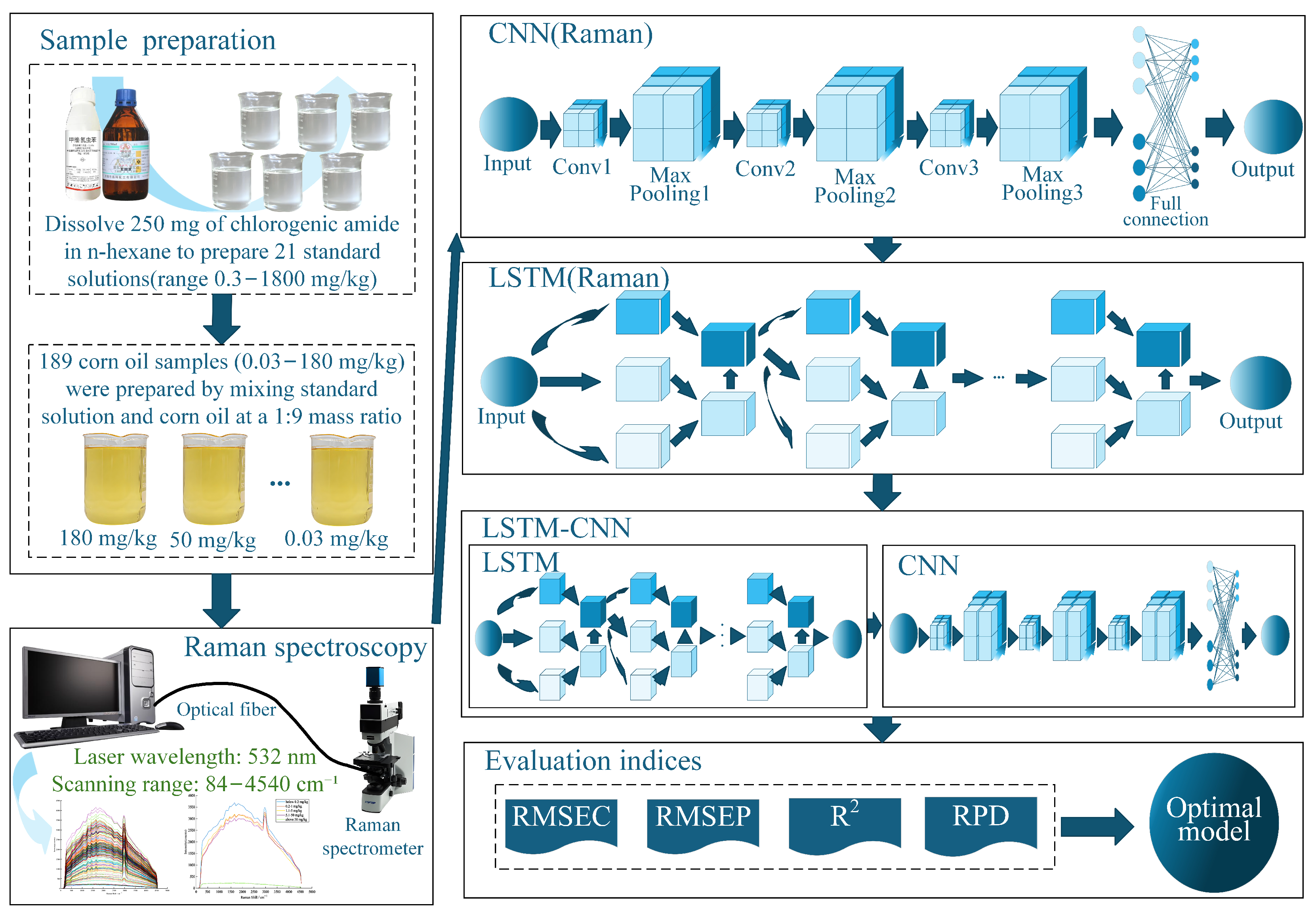
Hybrid DL models represent the frontier for processing complex spectral signatures. Xue et al. [61] devised an LSTM-CNN fusion network for chlorpyrifos detection in corn oil, where LSTM layers extracted sequential features from raw Raman spectra (84–4540 ${\mathrm{cm}}^{-1}$) and CNN blocks calibrated spatial dependencies. This end-to-end approach achieved superior performance ($RMSEP$ = 12.3 mg/kg, $RPD$ = 3.2) over standalone CNN or LSTM models by simultaneously capturing temporal-spectral correlations and spatial patterns without preprocessing. To make it clear, we present its schematic diagram in Figure 3 and core algorithm in Appendix A.1, as a representative example of DL research for contaminant detection. Despite these advances, computational efficiency and field adaptability remain critical challenges. Future efforts should prioritize lightweight architectures like MobileNetV3 for edge deployment, attention mechanisms for interpretable feature weighting, and multi-residue detection frameworks to address real-world contamination scenarios.

The pollution problem of plastic shopping bags in cotton fields is equally serious. If they are not removed before harvest, they will seriously affect the quality of fibers and disrupt the ginning operation. Yadav et al. [62] employed unmanned aerial vehicle (UAV)-captured RGB imagery and four variants of the YOLOv5 deep learning model $(s,m,l,x)$ to detect and locate plastic bags in real time, significantly improving upon traditional methods’ limited accuracy (64%) and processing delays. By manually placing 180 bags (90 white, 90 brown) at three heights on cotton plants and evaluating model performance through a desirability function, they demonstrated that YOLOv5 achieved 92% accuracy for white bags and 78% for brown bags (mAP@50: 88%), with color and height profoundly impacting detection—white bags outperformed brown due to contrast ($p<0.001$), while detection rates plummeted from 94.25% (top) to 5% (bottom) because of occlusion ($p<0.0001$). The YOLOv5 variant emerged as optimal (95% desirability, 86 FPS), balancing speed and accuracy, though larger models ($l/x$) underperformed due to insufficient training convergence. The framework enables near-real-time field deployment, with future work targeting edge-device implementation for robotic removal.

Last but not least, recent research [63,64] also demonstrates the versatility of DL in detecting diverse physical contaminants within agricultural products, utilizing advanced sensing modalities beyond conventional imaging. Alsaid et al. [63] explored the application of electrical impedance tomography (EIT) combined with CNNs for detecting hidden physical contaminants (plastic, stones, foreign food objects) embedded within fresh food products like chicken breast. Their approach leverages EIT’s ability to capture internal conductivity variations, overcoming limitations of surface-only inspection techniques when dealing with irregular shapes and sizes. Four dedicated CNNs were trained for binary classification (contaminated vs. clean), achieving promising accuracies (78–92.9%) for specific contaminant types and mixtures, showcasing EIT’s unique capability for internal anomaly detection, albeit with longer measurement times (15–20 min/sample). Complementing this, Lee et al. [64] addressed the critical challenge of detecting unknown or rare contaminants in food inspection lines using HSI. They propose the Partial and Aggregate Autoencoder (PA2E), a novel anomaly detection architecture specifically optimized for HSI spectral data. PA2E overcomes limitations of standard autoencoders (lacking locality) and convolutional layers (suffering from translation invariance) by employing masked fully connected layers to learn local spectral features without invariance, coupled with efficient global feature aggregation. Crucially, PA2E is engineered for real-time inference (0.53 ms/sample) through techniques like ReLU culling and layer fusion, significantly outperforming state-of-the-art anomaly detection methods (detecting 29 vs. avg. 23 out of 42 contaminants) on datasets like almonds, pistachios, and garlic stems. This makes PA2E particularly suitable for industrial settings requiring high-speed detection of unforeseen contaminants where labeled anomaly data is scarce.

Table 1. Contaminant, sample and technique analysis of DL applications in agricultural contaminant detection.

Reference	Contaminant	Sample	Technique
[57]	Heavy Metals	Fish	ELM + Colorimetric sensors
[2]	Heavy Metals	Lettuce	PSO-DBN
[58]	Heavy Metals	Lettuce	WT-SCAE
[59]	Mycotoxin	Maize	MTF-CNN
[60]	Pesticides	Tea	Au-Ag OHCs + 1D-CNN
[61]	Pesticides	Corn oil	LSTM-CNN
[62]	Plastic shopping bags	Cotton plants	YOLOv5
[63]	Plastic fragments, stone fragments, etc.	Chicken breast	EIT + CNN
[64]	Plastics, rubber, paper, metal, etc.	Almond, pistachio, garlic stems	HSI + PA2E

and

Table 2. Efficiency, accuracy and cost comparison among DL applications in agricultural contaminant detection.

Reference	Efficiency	Accuracy	Cost
[57]	Fast colorimetric measurements with 5-minute reaction time	Correlation coefficients: 0.854 for Pb, 0.83 for Cd, 0.845 for Hg); $RMSEP$: 0.102 mg/kg (Pb), 0.026 mg/kg (Cd), and 0.016 mg/kg (Hg)	Low-cost materials, Consumer-grade flatbed scanner
[2]	Rapid HSI with 618 bands, automated data processing	$R^2$ = 0.9234, $RMSEP$ = 0.5423 mg/kg, $RPD$ = 3.5894	Commercial hyperspectral camera with displacement platform
[58]	Automated HSI with 478 bands, rapid WT-SCAE feature extraction	$R^2$: 0.9319 for Cd, 0.9418 for Pb; $RMSEP$: 0.04988 mg/kg for Cd, 0.04123 mg/kg for Pb	HSI system, GPU
[59]	Automated NIR spectral processing with MTF-CNN, rapid feature extraction)	$R^2$ = 0.9955; $RPD$ = 14.9386; $RMSEP$ = 1.36 $\mathsf{\mu }$ g/kg	HSI system
[60]	Rapid detection (seconds per sample); suitable for on-site analysis	$R^2$: 0.995 for thiram, 0.977 for pymetrozine	SERS substrate synthesis, characterization equipment, Portable Raman spectrometer
[61]	Rapid analysis (seconds per sample); suitable for batch processing	$RMSEP$ = 12.3 mg/kg, $R^2$ = 0.90, $RPD$ = 3.2	QE Pro Raman, spectrometer
[62]	High-speed detection (81–86 FPS); real-time capability with YOLOv5m	92% for white bags, 78% for brown bags, mAP@50: 88%	Unmanned ircraft system equipment and cloud computing costs
[63]	Measurement time of 15–20 min/sample; 6.81× speedup vs. traditional chirp signals	92.9%, 85%, 85% accuracy for plastic, stone, all contaminants	EIT device development
[64]	Real-time inference (0.53 ms/sample); 2.6× faster than SOTA	Avg. 29/42 contaminants detected	PA2E + Layer Fusion

summarize these DL studies for contaminant detection, from the aspects of contaminant, sample, technique, efficiency, accuracy and cost. These studies demonstrate that DL can achieve rapid, non-destructive identification of heavy metals (Pb, Cd, Hg) and pesticides with exceptional accuracy ($R^2$ up to 0.9955). DL is a transformative tool for detecting diverse agricultural contaminants, leveraging techniques like HSI [2,27,58,64], CSA [57], Raman spectroscopy [61], and surface-enhanced Raman scattering [60]. For physical contaminants, UAV-based YOLOv5 models enable real-time plastic detection in fields (81–86 FPS [62]), while AI-enhanced EIT identifies subsurface materials like plastic with 92.9% accuracy [63]. Innovative architectures, including MTF-CNN for aflatoxins [59], LSTM-CNN hybrids [61], and efficiency-optimized autoencoders (PA2E [64]), significantly outperform traditional lab methods in speed and cost efficiency after initial hardware investments.

However, critical challenges persist, including computational complexity limiting field deployment for some advanced models (WT-SCAE, MTF-CNN, EIT), variable performance with contaminant properties (e.g., color/height for plastics, material type for EIT), and the need for optimization towards edge computing and broader generalizability. Moreover, the “black-box” nature of complex models (e.g., WT-SCAE, DBN-PSO) hampers regulatory trust due to limited model explainability, with few studies incorporating explainable artificial intelligence (XAI) techniques (e.g., attention mechanisms) to clarify feature contributions or decision logic. Furthermore, reproducibility is hindered by a pervasive lack of standardized datasets and protocols, as studies rely on proprietary or context-specific data with inconsistent contamination levels, sensor parameters (e.g., HSI wavelength ranges), and preprocessing methods, obstructing direct benchmarking and scalability. Future progress necessitates integrating XAI frameworks alongside collaborative efforts to establish unified data curation and evaluation standards, bridging the gap between laboratory efficacy and field deployment.

3. DL for Quality and Nutritional Component Analysis

Recent advances in DL have revolutionized the quality and nutritional component analysis in agricultural products. A prominent study by Zhang et al. [9] established a high-efficiency paradigm for geographical origin tracing of Radix puerariae starch using Fourier transform near-infrared (FT-NIR) spectroscopy. Their three-stage framework—incorporating interval selection via synergy interval partial least squares (siPLS) and an innovative iteratively retaining informative variables (IRIV) algorithm—achieved 100% classification accuracy with only 10 characteristic wavelengths. This approach demonstrated the critical role of feature engineering in DL pipelines, where IRIV’s variable interaction mechanism could enhance deep feature extraction layers. The extreme lightweight model (utilizing ELM) validated a “less-but-better” philosophy, though computational costs and untapped DL alternatives like CNNs warrant further exploration.

Similarly, in green tea polyphenol quantification [65], a cost-effective colorimetric sensor combined with ant colony optimization (ACO)-ELM addressed limitations of destructive chemical methods [8]. By optimizing 7–10 key RGB features from a 3 × 3 porphyrin array, the model achieved a prediction correlation coefficient ($R_p$) of 0.8035. This “simple hardware + intelligent algorithm” framework democratized rapid screening (<10 min/sample), yet moderate accuracy compared to NIR spectroscopy highlighted opportunities for integrating multi-sensor data or replacing handcrafted features with CNN-based image analysis.

For fruit quality assessment, Xu et al. [66] pioneered the fusion of deep spectral features and biophysical parameters in Kyoho grapes. An unsupervised stacked autoencoder (SAE) extracted pixel-level features from HSI data, while physical size compensation significantly improved predictions for total soluble solids (TSS, $R^2=0.924$) and titratable acidity (TA, $R^2=0.922$). This study underscored DL’s capacity to overcome spatial interference in HSI but revealed GPU dependency and single-variety limitations. Future edge computing adaptations could enable field deployment.

Physiological trait monitoring in crops has also benefited from multimodal integration of DL. Elsherbiny et al. [67] introduced a meta-learning framework for IoT-enabled aeroponic lettuce, fusing novel 3D spectral indices (e.g., $ND{I}_{1162,706,706}$), thermal indicators, and environmental parameters. Gradient boosting machine (GBM)-back-propagation neural networks (BPNN) stacking achieved robust recognition of leaf relative humidity (LRH, $R^2$ = 0.875), Chl ($R^2$ = 0.886) and Nitrogen levels (N, $R^2$ = 0.930), leveraging 3D indices’ superiority over conventional 2D counterparts. Despite hardware cost barriers, the work demonstrated meta-learning’s potential for rapid cross-crop adaptation.

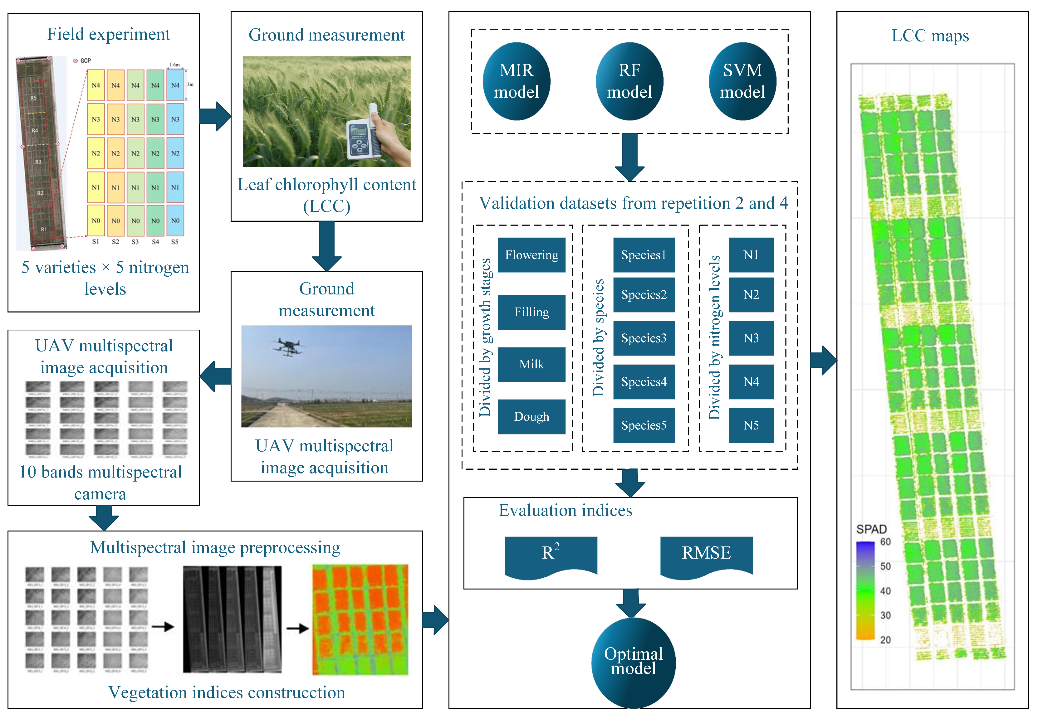
In Chl content estimation of winter wheat, Zhang et al. [12] systematically validated support vector machine (SVM) robustness across cultivars, nitrogen stresses, and growth stages using UAV multispectral data. SVM outperformed random forest (RF) and multiple linear regression (MLR), especially at dough stage ($R^2$ = 0.60 vs. 0.49 for RF), though water stress interference and underutilized red-edge bands remained challenges. To make it clear, we present its schematic diagram in Figure 4 and core algorithm in Appendix A.2. This study identified growth stage as the primary generalization bottleneck, advocating stage-specific models and multi-source data fusion.

Anthocyanin prediction in purple-leaf lettuce by Liu et al. [13] showcased optimized ELM enhanced by bio-inspired algorithms. A UVE-competitive adaptive reweighted sampling (CARS) feature selection pipeline compressed hyperspectral data to 12 key bands, while dung beetle optimizer (DBO) elevated ELM performance (validation $R^2$ = 0.8617). Three-band vegetation indices (e.g., Enhanced vegetation index (EVI)) surpassed two-band indices by 12.3% in $R^2$, emphasizing multispectral synergy in biochemical inversion. Computational load and field applicability limitations call for portable spectrometers and UAV integration.

Ahsan et al. [68] explored the application of DL for nutrient concentration assessment in hydroponic lettuce, achieving high accuracy (87.5–100%) in classifying nitrogen levels (0–300 ppm) across four cultivars using RGB images and transfer learning with VGG16/VGG19 architectures. This established the feasibility of DL for rapid monitoring of nutrients. Extending beyond direct RGB analysis, Ahmed et al. [69] addressed the limitations of HSI for real-time use by developing a DL-based reconstruction approach. Their hyperspectral convolutional neural network-dense (HSCNN-D) model successfully reconstructed hyperspectral images from standard RGB inputs for sweet potatoes, enabling accurate prediction of soluble solid content (SSC) via partial least squares regression (PLSR) models that outperformed those using full-spectrum HSI data. This highlights DL’s potential to democratize high-fidelity spectral analysis. For complex morphological phenotyping linked to yield quality, van Vliet et al. [70] tackled the data bottleneck in pod valve segmentation for Brassica napus. Their “DeepCanola” pipeline combined semi-synthetic data generation (using real pod annotations with programmatic augmentation and Thompson-inspired shape transformations) and active learning with human-in-the-loop validation. This drastically reduced annotation effort (1000× faster than manual labeling) while producing a robust Mask R-CNN model capable of accurately measuring yield-relevant valve length ($R^2$ = 0.99) in both ordered and disordered scenes, even generalizing to related species. These studies showcase DL’s evolution from direct image classification to sophisticated data synthesis/reconstruction for efficient, non-destructive quality and nutritional trait analysis across diverse products.

Collectively, these recent advances demonstrate the transformative role of DL and integrated sensing technologies in enabling efficient, accurate, and increasingly accessible analysis of key quality and nutritional components in agricultural products, which are summarized in

Table 3. Target component, sample and technique analysis of DL applications in detecting quality and nutritional component.

Reference	Target Component(s)	Sample	Technique
[9]	Geographical origin	Radix puerariae starch	FT-NIR + siPLS-IRIV-ELM (Interval selection → feature extraction)
[8]	Tea polyphenols	Green tea	Colorimetric sensor (porphyrin array) + ACO-ELM
[66]	TSS and TA	Kyoho grapes	HSI (400–1001 nm) + SAE-least squares SVM
[67]	LRH, Chlorophyll, Nitrogen	Lettuce (aeroponic)	Meta-learning (GBM-BPNN) multimodal fusion (3D-SRIs + thermal + IoT)
[12]	Leaf Chl Content	Winter wheat	UAV multispectral (10 bands) + SVM/MLR/RF multi-factor validation
[13]	Anthocyanins	Purple-leaf lettuce leaves	HSI + UVE-CARS + DBO + EVI
[68]	Nitrogen concentration	Four hydroponic lettuce cultivars	VGG16/19
[69]	SSC	Sweet potato	RGB-to-HSI reconstruction via HSCNN-D + PLSR
[70]	Pod valve length (yield-related trait)	Brassica napus pods (canola/rapeseed), Arabidopsis thaliana, Alliaria petiolata, Raphanus raphanistrum	Semi-synthetic data generation + Active learning (Mask R-CNN instance segmentation); Human-in-the-loop validation

and

Table 4. Efficiency, accuracy and cost comparison among DL applications in detecting quality and nutritional components.

Reference	Efficiency	Accuracy	Cost
[9]	Rapid spectral acquisition and automated variable selection (IRIV)	100% identification rate	High-end FT-NIR spectrometer
[8]	Manual sensor preparation and rapid screening (<10 min/sample)	$R_p$ = 0.8035, $RMSEP$ = 1.60039	Self-developed sensor, avoiding chemical reagents
[66]	SAE on pixel spectra (112 k); GPU-accelerated; size compensation	TSS: $R^2$ = 0.924, $RPD$ = 3.25; TA: $R^2$ = 0.922, $RPD$ = 3.21	HSI system, GPU
[67]	Real-time, non-invasive monitoring using IoT and meta-learning-driven data fusion	$R^2$ = 0.875 for LRH, 0.886 for Chl, 0.930 for N	Highspectrum data acquisition system, thermal imager
[12]	UAV-based multispectral imaging, enabling rapid data collection across large fields and multiple growth stages	$R^2$ = 0.93–0.95 for top VIs	Not specified
[13]	Non-destructive, suitable for rapid field/lab screening	$R^2$ = 0.8617, RMSE = 0.0095 mg/g, $RPD$ = 2.7192	Hyperspectral instrumentation
[68]	Trained on local machine (RTX-2080 GPU) in 85 s/epoch	VGG16/19: 97.9% avg. (87.5–100%	Not specified
[69]	Enables potential real-time, low-cost assessment using consumer cameras	$R^2$ = 0.6932, $RPD$ = 1.8054	Low-cost approach (compared to traditional HSI)
[70]	1000× faster data collection vs. manual annotation (39 vs. 996 person-hours for 44,823 annotations); Automated valve length extraction in seconds/image	Ordered pods: $R^2$ = 0.9930 (length), $R^2$ = 0.9966 (valve length); Disordered pods: $R^2$ = 0.9597 (length); Treatment effect significance: 100% agreement (p < 0.01) with manual measurements	Low-cost annotation, semi-synthetic generation

. Studies leveraging DL with diverse data sources—HSI for grape TSS/TA [66], UAV multispectral for wheat Chl [12], RGB images for lettuce nutrients [68], and even reconstructed HSI from RGB for sweet potato SSC [69]—consistently report high accuracy (often $R^2$ > 0.90 or accuracy > 87.5%) and efficiency gains over traditional methods. These approaches automate complex feature extraction (e.g., SAE for HSI pixels), enable rapid large-scale monitoring (e.g., via UAVs), and reduce long-term operational costs through minimized labor and targeted interventions. Meta-learning [67] and hybrid strategies combining DL with active learning/semi-synthetic data [70] further enhance robustness and reduce annotation burdens.

However, critical challenges remain. First, the inherent “black-box” nature of complex DL models like SAEs, CNNs (VGG16/19), and Mask R-CNN raises significant concerns regarding model explainability. Understanding why these models make specific predictions about component concentration or quality traits is crucial for building trust, diagnosing errors (e.g., accuracy drops during wheat dough stage), and enabling actionable insights for growers and regulators; yet, explicit discussion and application of XAI techniques within these agricultural DL studies are notably lacking. Second, the field suffers from a pronounced lack of standardized datasets and protocols. Research utilizes vastly different data types (pixel spectra, UAV images, RGB photos), acquisition settings, preprocessing methods, cultivar selections, and growth stage definitions. This heterogeneity severely hampers reproducibility, fair benchmarking of model performance, and the development of universally applicable solutions, limiting the broader adoption and scalability of these otherwise promising DL technologies. Third, there are some other challenges, including initial equipment costs (FT-NIR, HSI), model robustness across diverse conditions (growth stages, occlusion), and accuracy optimization for some sensor-based methods. Future directions should focus on building refined model architectures while being interpretable and establishing strict, community-agreed standards for data collection and annotation. There is also a need to enhance accessibility through portable devices, refine algorithms (e.g., exploring transformers for occlusion) and optimize sensor materials. By extending these frameworks to a wider set of components and crop types, scalable and intelligent precision agriculture will be necessary.

4. DL for Structural/Textural and Biotic Stress Assessment

DL techniques have demonstrated significant efficacy in the non-destructive assessment of agricultural product textures. For deep-fried tofu, Xuan et al. [11] proposed a novel framework, which integrated discrete wavelet transform (DWT) denoising with Light Gradient Boosting Machine (LightGBM) regression achieved high-precision texture prediction, yielding determination coefficients of 0.969 for resilience and 0.956 for cohesion. This approach leveraged ultrasonic echoes processed through PCA for dimensionality reduction, outperforming XGBoost and RF while visualizing spatial heterogeneity in porous structures.

Similarly, in minced chicken gel systems, Nunekpeku et al. [10] combined multimodal fusion of NIR and Raman spectroscopy with LSTM networks to decode complex gelation dynamics. Ultrasonic pretreatment optimized to 30 min enhanced protein $\beta$-sheet formation, and low-level data fusion enabled the LSTM model to attain unprecedented accuracy ($R^2$=0.9882, $RPD$=9.2091), capturing nonlinear relationships between spectral sequences and gel strength. Both studies highlight the critical role of signal preprocessing and sensor fusion in overcoming noise interference inherent to heterogeneous agricultural matrices. To make it clear, we present its schematic diagram in Figure 5 and core algorithm in Appendix A.3. This can serve as a representative example of DL research for structural/textural and biotic stress assessment.

For plant disease and weed management, DL models address key challenges in real-time field deployment. In strawberry cultivation, Liu et al. [71] designed a VGG16-based variable-rate spraying system to achieve targeted weed control with 93% coverage accuracy at speeds ≤ 3 km/h, reducing agrochemical usage by over 30% through low-cost cameras and solenoid valves. However, performance declined sharply beyond 3 km/h due to motion blur, revealing a fundamental speed–accuracy trade-off in dynamic environments.

To enhance disease diagnosis efficiency, Peng et al. [72] extracted fused deep features from pretrained CNNs (e.g., ResNet50 + ResNet101), and combined it with SVM to accelerate grape leaf disease classification to under 1 sec/inference while maintaining 99.81% F1-score—a 1000× speedup over end-to-end CNNs.

For tomato leaf diseases, Zhao et al. [73] proposed an SE-ResNet50 model embedding channel attention mechanisms (SENet), which improved small-lesion recognition to a 96.81% accuracy by amplifying discriminative features and suppressing background noise, outperformed vanilla ResNet50 by 4.25%. This model also exhibited exceptional cross-crop generalizability, attaining 99.24% accuracy on grape leaf datasets.

For cucumber leaf diseases, Khan et al. [74] present an automated framework for recognizing six cucumber leaf diseases (angular leaf spot, anthracnose, blight, downy mildew, powdery mildew, cucumber mosaic) using DL and feature selection. To address data imbalance and limited samples, the authors applied augmentation techniques (horizontal/vertical flips, 45°/60° rotations) to expand the dataset. Four pre-trained models (VGG16, ResNet50, ResNet101, DenseNet201) were fine-tuned, with DenseNet201 achieving the highest accuracy. A novel Entropy–ELM feature selection method was proposed to eliminate redundant features, followed by a parallel fusion approach to combine optimal features from individual and fused models. The framework achieved 98.48% accuracy using Cubic SVM, outperforming existing methods while reducing computational time.

For wheat leaf disease, Xu et al. [75] proposed an integrated DL framework for wheat leaf disease identification, combining parallel CNNs, residual channel attention blocks (RCAB), feedback blocks (FB), and elliptic metric learning (EML). The model achieves 99.95% accuracy on a proprietary dataset (7239 images across 5 classes) and maintains >98% accuracy on public datasets (CGIAR, Plant Diseases, LWDCD 2020). Key innovations include dual-path feature extraction for healthy/diseased leaves, channel-aware feature optimization via RCAB, iterative feature refinement through FB, and redundancy reduction using EML for precise classification. While demonstrating state-of-the-art performance over models like VGG19 and EfficientNet-B7, the authors note limitations in generalizing across ecological variations and wheat cultivars, suggesting future integration of hyperspectral data for enhanced robustness.

Complementing these approaches, Zhu et al. [76] integrated AlexNet, VGG, and ResNet features to propose a Multi-Model Fusion Network (MMFN) via transfer learning, which achieved 98.68% accuracy for citrus disease classification, leveraging complementary feature representations to distinguish subtle inter-class variations such as canker and greasy spot. Shafik et al. [77] introduced AgarwoodNet, a lightweight DL model designed for multi-plant biotic stress classification and detection to support sustainable agriculture. Addressing the limitations of heavy DL models (e.g., high computational costs and memory constraints), the authors developed a resource-efficient CNN using depth-wise separable convolutions and residual connections. The model was trained on two novel datasets: the agarwood pest and disease dataset (APDD) with 5,472 images (14 classes) from Brunei, and the turkey plant pests and diseases (TPPD) dataset with 4447 images (15 classes). AgarwoodNet achieved high accuracy (96.66–98.59% on APDD; 95.85–96.84% on TPPD) while maintaining a compact size of 37 MB, enabling deployment on low-memory edge devices for real-time field applications.

These recent advances in DL demonstrate significant potential for assessing structural/textural properties and biotic stress in agricultural products, which are summarized in

Table 5. Target application and technique analysis of DL applications in structural/textural and biotic stress assessment.

Reference	Target Application	Technique
[11]	Texture prediction (deep-fried tofu)	Ultrasonic detection + DWT denoising; LightGBM regression
[10]	Gel strength prediction (chicken mince)	NIR-Raman fusion + LSTM; Data augmentation (10× sample expansion)
[71]	Targeted weed control (strawberry fields)	VGG16 CNN for real-time weed detection; Arduino-controlled spraying system
[72]	Grape leaf disease diagnosis	Fused CNN features (AlexNet/GoogLeNet/ResNet); SVM classification with canonical correlation analysis (CCA)/direct fusion
[73]	Tomato disease diagnosis	SE-ResNet50 with attention module; Data augmentation (22k images)
[74]	Cucumber leaf disease classification	Entropy-ELM feature selection+Parallel feature fusion
[75]	Wheat leaf disease identification	RFE-CNN’s hybrid architecture (RCAB + FB + EML)
[76]	Citrus disease classification	MMFN: Fusion of AlexNet/ VGG/ ResNet; Feature stitching + transfer learning
[77]	Multi-plant biotic stress classification	Lightweight CNN (AgarwoodNet) with depth-wise separable convolutions, residual connections, and inception modules

and

Table 6. Efficiency, accuracy and cost comparison among DL applications in structural/textural and biotic stress assessment.

Reference	Efficiency	Accuracy	Cost
[11]	Rapid ultrasonic detection and LightGBM model training	$R^2$: 0.969 (resilience) and 0.956 (cohesion)	Ultrasonic system, texture analyzer
[10]	Rapid spectral data acquisition and LSTM model training	$R^2$ = 0.9882, $RPD$ = 9.2091	High-end spectroscopic instruments, ultrasonic processors, texture analyzers, and refrigerated centrifuges
[71]	Real-time weed classification and targeted spraying; performance decreases at speeds > 3 km/h due to blurry images	97% validation, 89% field	Custom-built electric sprayer chassis, webcams, solenoid valves, GPU; Training three CNN models on 12,443 images using TensorFlow framework
[72]	SVM training time < 1 s, real-time deployment potential	99.81% F1-score	High-performance workstation
[73]	Fast convergence (150 epochs) and real-time diagnosis (31.68 ms/image)	tomato diseases (10-class): 96.81%, grape diseases (5-class): 99.24%	Low-cost SE-ResNet50, suitable for resource-limited agricultural settings
[74]	Feature selection reduced processing time by 68% (vs. full features)	98.48%	Entropy–ELM feature selection, suitable for edge devices in field conditions
[75]	Short time consumption, adaptive ability	Overall accuracy: 98.83%	Not specified
[76]	Rapid processing of large datasets and model fusion	healthy/unhealthy leaves: 99.72%, multi-disease classification: 98.68%	Transfer learning, automated classification
[77]	Model size: 37 MB; Inference time: 2.93–3.93 s; Optimized for low-memory devices	APDD: 96.66–98.59%, TPPD: 95.85–96.84%	Not specified

. Studies highlight the efficiency, cost effectiveness, and high accuracy (often >95–99%) of DL models like VGG16, SE-ResNet50, MMFN, and lightweight architectures (e.g., AgarwoodNet) in tasks such as targeted weed/spray control, disease diagnosis across crops (strawberry, grape, tomato, citrus, wheat, cucumber), and texture prediction (e.g., deep-fried tofu, chicken gel). Innovations like attention mechanisms (e.g., SENet [38,39]), fused deep features (e.g., direct concatenation [78], CCA [79,80]) and ensemble methods enhance feature extraction, reduce computational costs, and enable near-real-time processing, facilitating field deployment.

However, critical limitations persist. First, model explainability remains largely unaddressed. While attention modules (e.g., SE-ResNet50) offer basic interpretability by highlighting relevant features, deeper exploration of XAI techniques (e.g., Shapley additive explanations (SHAP), local interpretable model-agnostic explanations (LIME)) is essential to build trust, understand decision logic, and refine models for complex agricultural environments. Second, the lack of standardized datasets and protocols hampers reproducibility and benchmarking. Performance variations across plant varieties (e.g., wheat), ecological conditions, and datasets (e.g., cross-domain drops in AgarwoodNet), coupled with challenges from data imbalance (e.g., minority disease classes) and dynamic field conditions (lighting, occlusion), underscore the need for large-scale, diverse, and consistently annotated benchmark datasets. Third, challenges persist in balancing speed–accuracy trade-offs, generalizing models across diverse environments, and adapting DL systems to resource-constrained edge devices. Future work must prioritize XAI integration and collaborative efforts toward standardized data collection and evaluation frameworks to ensure robustness and scalability. Simultaneously, lightweight model optimization, multimodal data integration, and cross-species adaptability are also critical to advance scalable precision agriculture.

5. Challenges and Future Directions

This review categorizes DL applications in detecting special components of agricultural products into three primary domains. Firstly, DL for contaminant detection focuses on identifying foreign materials and hazardous substances, utilizing advanced image analysis and spectral data processing to enhance food safety inspection. Secondly, DL for quality and nutritional component analysis leverages non-invasive techniques like HSI and computer vision to rapidly and accurately quantify internal quality attributes, ripeness, and nutritional value, overcoming limitations of traditional destructive methods. Finally, DL for structural/textural and biotic stress assessment employs high-throughput image analysis to evaluate surface features, texture, and physical damage, while also enabling early and precise detection of pest infestations, diseases, and other biotic stresses affecting crop health and marketability. Collectively, these DL approaches offer transformative capabilities for automated, objective, accurate and efficient assessment across the agricultural product value chain.

Despite significant advancements in DL for agricultural component detection, several persistent challenges impede widespread deployment. Foremost, the pervasive “black-box” nature of complex models (e.g., WT-SCAE, DBN-PSO, SAEs, Mask R-CNN, SE-ResNet50) severely limits explainability and regulatory trust, as critical spectral features identified by networks (e.g., key wavelengths for heavy metal detection) often lack clear biophysical justification, hindering scientific validation and user trust. Few schemes adopt XAI techniques (e.g., attention, SHAP, LIME) to clarify decision logic or feature contributions. Second, reproducibility and scalability are crippled by a pronounced lack of standardized datasets, protocols, and benchmarking frameworks. Studies rely on fragmented, context-specific data with inconsistencies in contamination levels, sensor parameters (HSI wavelengths, FT-NIR), acquisition settings, preprocessing methods, crop varieties, growth stages, and annotation criteria. Most DL frameworks exhibit substantial performance degradation when confronted with variations in crop cultivars, growth stages, or environmental conditions, as evidenced by [12] on wheat Chl prediction where model accuracy dropped by over 60% during the dough stage compared to flowering. This fragility stems from insufficient training data representing agricultural heterogeneity and the inherent complexity of biotic/abiotic interactions in field environments. Third, computational inefficiency further constrains real-time applications, particularly for resource-intensive architectures like 3D-CNNs and hybrid models (e.g., CNN-LSTM), which require specialized hardware (e.g., GPUs) and struggle with latency requirements for field-deployable systems. Moreover, challenges also exist in balancing speed–accuracy trade-offs, achieving robustness across variable field conditions (occlusion, lighting, biotic stresses), generalizing models across environments/species, and adapting advanced architectures to resource-constrained edge devices. Additional hurdles include high equipment costs, data imbalance (minority disease classes), and performance sensitivity to contaminant properties or component variability. Specifically, the dependency on controlled laboratory settings for data acquisition—where samples are meticulously prepared under optimal conditions—fails to capture the sensor noise, occlusion, and lighting variability endemic to real-world agricultural operations.

Future progress necessitates integrated strategies addressing core limitations. First, the systematic incorporation of XAI frameworks (e.g., attention mechanisms, SHAP, LIME) is essential to demystify model reasoning, build trust, and enable actionable diagnostics. Embedding domain-specific physical knowledge into DL architectures will enhance robustness and interpretability. Techniques like physics-guided feature weighting (e.g., prioritizing chlorophyll-sensitive bands in Cd-stressed crops) or coupling mechanistic models (e.g., protein denaturation kinetics in thermal processing) with neural networks could bridge data-driven predictions and agricultural principles [81]. Second, establishing large-scale benchmark datasets and standardized validation protocols for cross-crop, cross-environment model testing is essential to reproducibility and fair benchmarking. Transfer learning leveraging agricultural foundation models, alongside federated learning frameworks for distributed farm data, will accelerate the transition from lab-validated prototypes to field-ready solutions capable of addressing global food safety and quality challenges. Third, developing lightweight architectures (e.g., knowledge-distilled CNNs, attention-optimized MobileNetV3) compatible with edge devices will enable real-time field deployment, as demonstrated in Deng et al.’s miniaturized microwave sensor for lead detection in edible oils [5]. Integrating multimodal data fusion represents another critical pathway, where complementary sensing technologies—such as HSI combined with IoT environmental parameters or Raman spectroscopy [82] paired with ultrasonic metrics—can compensate for individual modality limitations. Osama et al.’s meta-learning framework for lettuce physiology monitoring exemplifies this approach [67], synergizing 3D spectral indices with microclimate data to achieve $R^2>0.88$ for Chl and nitrogen prediction. Extending validated frameworks to diverse components and crop types, alongside sensor material innovation, will be critical for scalable, intelligent precision agriculture.

6. Conclusions

This comprehensive review demonstrates the transformative potential of DL in revolutionizing the detection and analysis of special components within agricultural products. Across diverse applications—from contaminant surveillance to quality attribute assessment—DL techniques have consistently outperformed traditional methods by overcoming inherent limitations of high-dimensional data processing, nonlinear feature extraction, and environmental interference. The integration of advanced neural architectures with novel sensing modalities (e.g., e.g., SERS [6,60,83], HSI [14,66,84], microwave [5,47]) has enabled unprecedented sensitivity in detecting trace-level hazards such as heavy metals, pesticides, and mycotoxins, while simultaneously providing non-destructive quantification of nutritional metabolites and physiological indicators.

Critically, the evolution of specialized DL frameworks—including attention-enhanced networks for lesion localization, wavelet-coupled autoencoders for spectral denoising, and multi-task learning for joint parameter prediction—has addressed fundamental challenges in agricultural diagnostics. Future progress requires prioritizing the integration of XAI, establishing standardized cross-domain datasets and protocols, and developing lightweight, edge-compatible models alongside multimodal data fusion to enable robust, scalable precision agriculture.

References

1. Wu, M.; Sun, J.; Lu, B.; Ge, X.; Zhou, X.; Zou, M. Application of deep brief network in transmission spectroscopy detection of pesticide residues in lettuce leaves. J. Food Process Eng. 2019, 42, e13005. [Google Scholar] [CrossRef]
2. Sun, J.; Wu, M.; Hang, Y.; Lu, B.; Wu, X.; Chen, Q. Estimating cadmium content in lettuce leaves based on deep brief network and hyperspectral imaging technology. J. Food Process Eng. 2019, 42, e13293. [Google Scholar] [CrossRef]
3. Cheng, J.; Sun, J.; Yao, K.; Xu, M.; Wang, S.; Fu, L. Hyperspectral technique combined with stacking and blending ensemble learning method for detection of cadmium content in oilseed rape leaves. J. Sci. Food Agric. 2023, 103, 2690–2699. [Google Scholar] [CrossRef] [PubMed]
4. Zhou, X.; Zhao, C.; Sun, J.; Cao, Y.; Yao, K.; Xu, M. A deep learning method for predicting lead content in oilseed rape leaves using fluorescence hyperspectral imaging. Food Chem. 2023, 409, 135251. [Google Scholar] [CrossRef] [PubMed]
5. Deng, J.; Ni, L.; Bai, X.; Jiang, H.; Xu, L. Simultaneous analysis of mildew degree and aflatoxin B1 of wheat by a multi-task deep learning strategy based on microwave detection technology. LWT 2023, 184, 115047. [Google Scholar] [CrossRef]
6. Adade, S.Y.S.S.; Lin, H.; Nunekpeku, X.; Johnson, N.A.N.; Agyekum, A.A.; Zhao, S.; Teye, E.; Qianqian, S.; Kwadzokpui, B.A.; Ekumah, J.N.; et al. Flexible paper-based AuNP sensor for rapid detection of diabenz (a,h)anthracene (DbA) and benzo(b)fluoranthene (BbF) in mussels coupled with deep learning algorithms. Food Control 2025, 168, 110966. [Google Scholar] [CrossRef]
7. Tian, Y.; Sun, J.; Zhou, X.; Yao, K.; Tang, N. Detection of soluble solid content in apples based on hyperspectral technology combined with deep learning algorithm. J. Food Process. Preserv. 2022, 46, e16414. [Google Scholar] [CrossRef]
8. Jiang, H.; Xu, W.; Chen, Q. Determination of tea polyphenols in green tea by homemade color sensitive sensor combined with multivariate analysis. Food Chem. 2020, 319, 126584. [Google Scholar] [CrossRef]
9. Zhang, H.; Jiang, H.; Liu, G.; Mei, C.; Huang, Y. Identification of Radix puerariae starch from different geographical origins by FT-NIR spectroscopy. Int. J. Food Prop. 2017, 20, 1567–1577. [Google Scholar] [CrossRef]
10. Nunekpeku, X.; Zhang, W.; Gao, J.; Adade, S.Y.S.S.; Li, H.; Chen, Q. Gel strength prediction in ultrasonicated chicken mince: Fusing near-infrared and Raman spectroscopy coupled with deep learning LSTM algorithm. Food Control 2025, 168, 110916. [Google Scholar] [CrossRef]
11. Xuan, L.; Lin, Z.; Liang, J.; Huang, X.; Li, Z.; Zhang, X.; Zou, X.; Shi, J. Prediction of resilience and cohesion of deep-fried tofu by ultrasonic detection and LightGBM regression. Food Control 2023, 154, 110009. [Google Scholar] [CrossRef]
12. Zhang, L.; Wang, A.; Zhang, H.; Zhu, Q.; Zhang, H.; Sun, W.; Niu, Y. Estimating Leaf Chlorophyll Content of Winter Wheat from UAV Multispectral Images Using Machine Learning Algorithms under Different Species, Growth Stages, and Nitrogen Stress Conditions. Agriculture 2024, 14, 1064. [Google Scholar] [CrossRef]
13. Liu, C.; Yu, H.; Liu, Y.; Zhang, L.; Li, D.; Zhang, J.; Li, X.; Sui, Y. Prediction of Anthocyanin Content in Purple-Leaf Lettuce Based on Spectral Features and Optimized Extreme Learning Machine Algorithm. Agronomy 2024, 14, 2915. [Google Scholar] [CrossRef]
14. You, J.; Li, D.; Wang, Z.; Chen, Q.; Ouyang, Q. Prediction and visualization of moisture content in Tencha drying processes by computer vision and deep learning. J. Sci. Food Agric. 2024, 104, 5486–5494. [Google Scholar] [CrossRef]
15. Dong, M. HPLC Applications in Food, Environmental, Chemical, and Life Sciences Analysis. In HPLC and UHPLC for Practicing Scientists; John Wiley & Sons, Ltd.: Hoboken, NJ, USA, 2019; Chapter 13; pp. 335–369. [Google Scholar] [CrossRef]
16. Hill, C.; Roessner, U. Metabolic Profiling of Plants by GC-MS; John Wiley & Sons, Inc.: Hoboken, NJ, USA, 2013. [Google Scholar] [CrossRef]
17. Adebo, O.A.; Oyeyinka, S.A.; Adebiyi, J.A.; Feng, X.; Wilkin, J.D.; Kewuyemi, Y.O.; Abrahams, A.M.; Tugizimana, F. Application of gas chromatography–mass spectrometry (GC-MS)-based metabolomics for the study of fermented cereal and legume foods: A review. Int. J. Food Sci. Technol. 2020, 56, 1514–1534. [Google Scholar] [CrossRef]
18. Min, X.; Xu, H.; Huang, F.; Wei, Y.; Lin, W.; Zhang, Z. GC-MS-based metabolite profiling of key differential metabolites between superior and inferior spikelets of rice during the grain filling stage. BMC Plant Biol. 2021, 439, 15. [Google Scholar] [CrossRef] [PubMed]
19. Choudhury, F.; Pandey, P.; Meitei, R.; Cardona, D.; Gujar, A.; Shulaev, V. GC-MS/MS Profiling of Plant Metabolites; Humana: New York, NY, USA, 2022; Volume 2396, pp. 101–115. [Google Scholar] [CrossRef]
20. Kim, Y.K.; Baek, E.J.; Na, T.W.; Sim, K.S.; Kim, H.; Kim, H.J. LC–MS/MS and GC–MS/MS Cross-Checking Analysis Method for 426 Pesticide Residues in Agricultural Products: A Method Validation and Measurement of Uncertainty. J. Agric. Food Chem. 2024, 72, 22814–22821. [Google Scholar] [CrossRef] [PubMed]
21. Mazarakioti, E.C.; Zotos, A.; Thomatou, A.A.; Kontogeorgos, A.; Patakas, A.; Ladavos, A. Inductively Coupled Plasma-Mass Spectrometry (ICP-MS), a Useful Tool in Authenticity of Agricultural Products’ and Foods’ Origin. Foods 2022, 11, 3705. [Google Scholar] [CrossRef]
22. Langasco, I.; Barracu, F.; Deroma, M.A.; López-Sánchez, J.F.; Mara, A.; Meloni, P.; Pilo, M.I.; Sahuquillo Estrugo, À.; Sanna, G.; Spano, N.; et al. Assessment and validation of ICP-MS and IC-ICP-MS methods for the determination of total, extracted and speciated arsenic. Application to samples from a soil-rice system at varying the irrigation method. J. Environ. Manag. 2022, 302, 114105. [Google Scholar] [CrossRef]
23. Grothaus, G.; Bandla, M.; Currier, T.; Giroux, R.; Jenkins, G.; Lipp, M.; Shan, G.; Stave, J.; Pantella, V. Immunoassay as an Analytical Tool in Agricultural Biotechnology. J. AOAC Int. 2006, 89, 913–928. [Google Scholar] [CrossRef]
24. Schmidt, J.; Alarcon, C. Immunoassay Method Validation. In Immunoassays in Agricultural Biotechnology; John Wiley & Sons, Ltd.: Hoboken, NJ, USA, 2011; Chapter 6; pp. 115–138. [Google Scholar] [CrossRef]
25. Clapper, G.M.; Kurman, L. Immunoassay Applications in Grain Products and Food Processing. In Immunoassays in Agricultural Biotechnology; John Wiley & Sons, Ltd.: Hoboken, NJ, USA, 2011; Chapter 11; pp. 241–256. [Google Scholar] [CrossRef]
26. Du, M.; Yang, Q.; Liu, W.; Ding, Y.; Chen, H.; Hua, X.; Wang, M. Development of immunoassays with high sensitivity for detecting imidacloprid in environment and agro-products using phage-borne peptides. Sci. Total Environ. 2020, 723, 137909. [Google Scholar] [CrossRef]
27. Sun, J.; Cao, Y.; Zhou, X.; Wu, M.; Sun, Y.; Hu, Y. Detection for lead pollution level of lettuce leaves based on deep belief network combined with hyperspectral image technology. J. Food Saf. 2021, 41, e12866. [Google Scholar] [CrossRef]
28. Shi, Y.; Wang, Y.; Hu, X.; Li, Z.; Huang, X.; Liang, J.; Zhang, X.; Zhang, D.; Zou, X.; Shi, J. Quantitative characterization of the diffusion behavior of sucrose in marinated beef by HSI and FEA. Meat Sci. 2023, 195, 109002. [Google Scholar] [CrossRef]
29. Lu, B.; Sun, J.; Yang, N.; Hang, Y. Fluorescence hyperspectral image technique coupled with HSI method to predict solanine content of potatoes. J. Food Process. Preserv. 2019, 43, e14198. [Google Scholar] [CrossRef]
30. Zhang, Z.; Lu, Y.; Yang, M.; Wang, G.; Zhao, Y.; Hu, Y. Optimal training strategy for high-performance detection model of multi-cultivar tea shoots based on deep learning methods. Sci. Hortic. 2024, 328, 112949. [Google Scholar] [CrossRef]
31. Zhang, Z.; Yang, M.; Pan, Q.; Jin, X.; Wang, G.; Zhao, Y.; Hu, Y. Identification of tea plant cultivars based on canopy images using deep learning methods. Sci. Hortic. 2025, 339, 113908. [Google Scholar] [CrossRef]
32. Jothibasu, M.; Vallisa, R.; Abinaya, S.; Abishek, M. Deep Learning Models for Precision Agriculture: Evaluating CNN Architectures for Accurate Plant Disease Detection. In Proceedings of the 2025 International Conference on Computational Innovations and Engineering Sustainability (ICCIES), Coimbatore, India, 24–26 April 2025; pp. 1–7. [Google Scholar] [CrossRef]
33. Altalak, M.; Ammad uddin, M.; Alajmi, A.; Rizg, A. Smart Agriculture Applications Using Deep Learning Technologies: A Survey. Appl. Sci. 2022, 12, 5919. [Google Scholar] [CrossRef]
34. Zhang, P. Energy Detection using Savitzky-Golay Smoothing Method for Spectrum Sensing in Cognitive Radio. In Proceedings of the 2019 IEEE 8th Joint International Information Technology and Artificial Intelligence Conference (ITAIC), Chongqing, China, 24–26 May 2019; pp. 1181–1185. [Google Scholar] [CrossRef]
35. Yang, N.; Chang, K.; Dong, S.; Tang, J.; Wang, A.; Huang, R.; Jia, Y. Rapid image detection and recognition of rice false smut based on mobile smart devices with anti-light features from cloud database. Biosyst. Eng. 2022, 218, 229–244. [Google Scholar] [CrossRef]
36. Mateo-Sanchis, A.; Adsuara, J.E.; Piles, M.; Munoz-Marí, J.; Perez-Suay, A.; Camps-Valls, G. Interpretable Long Short-Term Memory Networks for Crop Yield Estimation. IEEE Geosci. Remote Sens. Lett. 2023, 20, 2501105. [Google Scholar] [CrossRef]
37. Sung, W.T.; Tofik Isa, I.G. The Improved Mango Plant Detection Model Based on Attention Module Mechanism. In Proceedings of the 2024 IEEE International Conference on Systems, Man, and Cybernetics (SMC), Kuching, Malaysia, 6–10 October 2024; pp. 1193–1194. [Google Scholar] [CrossRef]
38. Hu, J.; Shen, L.; Sun, G. Squeeze-and-Excitation Networks. In Proceedings of the 2018 IEEE/CVF Conference on Computer Vision and Pattern Recognition, Salt Lake City, UT, USA, 18–23 June 2018; pp. 7132–7141. [Google Scholar] [CrossRef]
39. Xing, S.; Tang, H. Combining Gated SENet with ResNet Backbone for Image Classification. In Proceedings of the 2024 36th Chinese Control and Decision Conference (CCDC), Xi’an, China, 25–27 May 2024; pp. 5927–5931. [Google Scholar] [CrossRef]
40. Joshi, P.; Das, D.; Udutalapally, V.; Misra, S.C. FarmEdge: A Unified Edge Computing Framework Enabling Digital Agriculture. In Proceedings of the 2021 IEEE International Symposium on Smart Electronic Systems (iSES), Jaipur, India, 18–22 December 2021; pp. 255–260. [Google Scholar] [CrossRef]
41. K, V.; Camargo, M.E.; Filho, W.P.; Sathiyanarayanan, M. Enhancing Personalized Agriculture With Cutting-Edge Hybrid Machine Learning Models And Intelligent Edge Computing For Sustainable Farming. In Proceedings of the 2025 International Conference on Data Science, Agents & Artificial Intelligence (ICDSAAI), Chennai, India, 28–29 March 2025; pp. 1–6. [Google Scholar] [CrossRef]
42. Yi, Y.; Li, R.; Chen, Z. Deep Meta-Learning with 1D-CNNs for Surface Deterioration Recognition of Overhead Conductors of Electricity Grid. IEEE Trans. Instrum. Meas. 2023, 72, 3500110. [Google Scholar] [CrossRef]
43. Sahu, P.; Jha, S.; Kumar, S. Optimized 1D CNNs for Enhanced Early Detection and Accurate Prediction of COPD and Other Pulmonary Diseases. In Proceedings of the 2024 IEEE Region 10 Symposium (TENSYMP), New Delhi, India, 27–29 September 2024; pp. 1–6. [Google Scholar] [CrossRef]
44. Athiramol, S.; Sudheep Elavidom, M. Enhanced MobileNet Architecture with Residual Blocks for Improved CT Image Classification. In Proceedings of the 2024 1st International Conference on Trends in Engineering Systems and Technologies (ICTEST), Kochi, India, 11–13 April 2024; pp. 1–5. [Google Scholar] [CrossRef]
45. Ou, L.; Zhu, K. Identification Algorithm of Diseased Leaves based on MobileNet Model. In Proceedings of the 2022 4th International Conference on Communications, Information System and Computer Engineering (CISCE), Shenzhen, China, 27–29 May 2022; pp. 318–321. [Google Scholar] [CrossRef]
46. Kaur, A.; Kukreja, V.; Thapliyal, N.; Manwal, M.; Sharma, R. Pre-trained MobileNet Model to Revolutionise Dermatological Diagnostics: A Multi-Class Skin Disease Detection. In Proceedings of the 2024 IEEE International Conference on Interdisciplinary Approaches in Technology and Management for Social Innovation (IATMSI), Gwalior, India, 14–16 March 2024; Volume 2, pp. 1–5. [Google Scholar] [CrossRef]
47. Deng, J.; Zhao, X.; Luo, W.; Bai, X.; Xu, L.; Jiang, H. Microwave detection technique combined with deep learning algorithm facilitates quantitative analysis of heavy metal Pb residues in edible oils. J. Food Sci. 2024, 89, 6005–6015. [Google Scholar] [CrossRef] [PubMed]
48. Kamilaris, A.; Prenafeta-Boldú, F.X. Deep learning in agriculture: A survey. Comput. Electron. Agric. 2018, 147, 70–90. [Google Scholar] [CrossRef]
49. Kaur, P.; Gautam, V. Research patterns and trends in classification of biotic and abiotic stress in plant leaf. Mater. Today Proc. 2021, 45, 4377–4382. [Google Scholar] [CrossRef]
50. Bouguettaya, A.; Zarzour, H.; Kechida, A.; Taberkit, A.M. Deep learning techniques to classify agricultural crops through UAV imagery: A review. Neural Comput. Appl. 2022, 34, 9511–9536. [Google Scholar] [CrossRef]
51. Attri, I.; Awasthi, L.K.; Sharma, T.P.; Rathee, P. A review of deep learning techniques used in agriculture. Ecol. Inform. 2023, 77, 102217. [Google Scholar] [CrossRef]
52. Albahar, M. A Survey on Deep Learning and Its Impact on Agriculture: Challenges and Opportunities. Agriculture 2023, 13, 540. [Google Scholar] [CrossRef]
53. Guerri, M.F.; Distante, C.; Spagnolo, P.; Bougourzi, F.; Taleb-Ahmed, A. Deep learning techniques for hyperspectral image analysis in agriculture: A review. ISPRS Open J. Photogramm. Remote Sens. 2024, 12, 100062. [Google Scholar] [CrossRef]
54. Waqas, M.; Naseem, A.; Humphries, U.W.; Hlaing, P.T.; Dechpichai, P.; Wangwongchai, A. Applications of machine learning and deep learning in agriculture: A comprehensive review. Green Technol. Sustain. 2025, 3, 100199. [Google Scholar] [CrossRef]
55. Krishnamoorthy, R.; Thiagarajan, R.; Padmapriya, S.; Mohan, I.; Arun, S.; Dineshkumar, T. Applications of Machine Learning and Deep Learning in Smart Agriculture. In Machine Learning Algorithms for Signal and Image Processing; John Wiley & Sons, Inc.: Hoboken, NJ, USA, 2023; pp. 371–395. [Google Scholar] [CrossRef]
56. Zhu, H.; Lin, C.; Liu, G.; Wang, D.; Qin, S.; Li, A.; Xu, J.L.; He, Y. Intelligent agriculture: Deep learning in UAV-based remote sensing imagery for crop diseases and pests detection. Front. Plant Sci. 2024, 15, 1435016. [Google Scholar] [CrossRef]
57. Han, F.; Huang, X.; Teye, E. Novel prediction of heavy metal residues in fish using a low-cost optical electronic tongue system based on colorimetric sensors array. J. Food Process Eng. 2019, 42, e12983. [Google Scholar] [CrossRef]
58. Zhou, X.; Sun, J.; Tian, Y.; Lu, B.; Hang, Y.; Chen, Q. Hyperspectral technique combined with deep learning algorithm for detection of compound heavy metals in lettuce. Food Chem. 2020, 321, 126503. [Google Scholar] [CrossRef]
59. Wang, B.; Deng, J.; Jiang, H. Markov Transition Field Combined with Convolutional Neural Network Improved the Predictive Performance of Near-Infrared Spectroscopy Models for Determination of Aflatoxin B1 in Maize. Foods 2022, 11, 2210. [Google Scholar] [CrossRef]
60. Li, H.; Luo, X.; Haruna, S.A.; Zareef, M.; Chen, Q.; Ding, Z.; Yan, Y. Au-Ag OHCs-based SERS sensor coupled with deep learning CNN algorithm to quantify thiram and pymetrozine in tea. Food Chem. 2023, 428, 136798. [Google Scholar] [CrossRef]
61. Xue, Y.; Jiang, H. Monitoring of Chlorpyrifos Residues in Corn Oil Based on Raman Spectral Deep-Learning Model. Foods 2023, 12, 2402. [Google Scholar] [CrossRef]
62. Yadav, P.K.; Thomasson, J.A.; Hardin, R.; Searcy, S.W.; Braga-Neto, U.; Popescu, S.C.; Rodriguez, R.; Martin, D.E.; Enciso, J.; Meza, K.; et al. Plastic Contaminant Detection in Aerial Imagery of Cotton Fields Using Deep Learning. Agriculture 2023, 13, 1365. [Google Scholar] [CrossRef]
63. Alsaid, B.; Saroufil, T.; Berim, R.; Majzoub, S.; Hussain, A.J. Food Physical Contamination Detection Using AI-Enhanced Electrical Impedance Tomography. IEEE Trans. AgriFood Electron. 2024, 2, 518–526. [Google Scholar] [CrossRef]
64. Lee, J.; Kim, M.; Yoon, J.; Yoo, K.; Byun, S.J. PA2E: Real-Time Anomaly Detection With Hyperspectral Imaging for Food Safety Inspection. IEEE Access 2024, 12, 175535–175549. [Google Scholar] [CrossRef]
65. Zhao, S.; Adade, S.Y.S.S.; Wang, Z.; Jiao, T.; Ouyang, Q.; Li, H.; Chen, Q. Deep learning and feature reconstruction assisted vis-NIR calibration method for on-line monitoring of key growth indicators during kombucha production. Food Chem. 2025, 463, 141411. [Google Scholar] [CrossRef] [PubMed]
66. Xu, M.; Sun, J.; Cheng, J.; Yao, K.; Wu, X.; Zhou, X. Non-destructive prediction of total soluble solids and titratable acidity in Kyoho grape using hyperspectral imaging and deep learning algorithm. Int. J. Food Sci. Technol. 2023, 58, 9–21. [Google Scholar] [CrossRef]
67. Elsherbiny, O.; Gao, J.; Ma, M.; Guo, Y.; Tunio, M.H.; Mosha, A.H. Advancing lettuce physiological state recognition in IoT aeroponic systems: A meta-learning-driven data fusion approach. Eur. J. Agron. 2024, 161, 127387. [Google Scholar] [CrossRef]
68. Ahsan, M.; Eshkabilov, S.; Cemek, B.; Küçüktopcu, E.; Lee, C.W.; Simsek, H. Deep Learning Models to Determine Nutrient Concentration in Hydroponically Grown Lettuce Cultivars (Lactuca sativa L.). Sustainability 2022, 14, 416. [Google Scholar] [CrossRef]
69. Ahmed, M.T.; Monjur, O.; Kamruzzaman, M. Deep learning-based hyperspectral image reconstruction for quality assessment of agro-product. J. Food Eng. 2024, 382, 112223. [Google Scholar] [CrossRef]
70. van Vliet, L.J.; Atkins, K.; Kurup, S.; Siles, L.; Hepworth, J.; Corke, F.M.; Doonan, J.H.; Lu, C. DeepCanola: Phenotyping brassica pods using semi-synthetic data and active learning. Comput. Electron. Agric. 2025, 237, 110470. [Google Scholar] [CrossRef]
71. Liu, J.; Abbas, I.; Noor, R.S. Development of Deep Learning-Based Variable Rate Agrochemical Spraying System for Targeted Weeds Control in Strawberry Crop. Agronomy 2021, 11, 1480. [Google Scholar] [CrossRef]
72. Peng, Y.; Zhao, S.; Liu, J. Fused-Deep-Features Based Grape Leaf Disease Diagnosis. Agronomy 2021, 11, 2234. [Google Scholar] [CrossRef]
73. Zhao, S.; Peng, Y.; Liu, J.; Wu, S. Tomato Leaf Disease Diagnosis Based on Improved Convolution Neural Network by Attention Module. Agriculture 2021, 11, 651. [Google Scholar] [CrossRef]
74. Khan, M.A.; Alqahtani, A.; Khan, A.; Alsubai, S.; Binbusayyis, A.; Ch, M.M.I.; Yong, H.S.; Cha, J. Cucumber Leaf Diseases Recognition Using Multi Level Deep Entropy-ELM Feature Selection. Appl. Sci. 2022, 12, 593. [Google Scholar] [CrossRef]
75. Xu, L.; Cao, B.; Zhao, F.; Ning, S.; Xu, P.; Zhang, W.; Hou, X. Wheat leaf disease identification based on deep learning algorithms. Physiol. Mol. Plant Pathol. 2023, 123, 101940. [Google Scholar] [CrossRef]
76. Zhu, H.; Wang, D.; Wei, Y.; Zhang, X.; Li, L. Combining Transfer Learning and Ensemble Algorithms for Improved Citrus Leaf Disease Classification. Agriculture 2024, 14, 1549. [Google Scholar] [CrossRef]
77. Shafik, W.; Tufail, A.; De Silva, L.; MohdApong, R. A lightweight deep learning model for multi-plant biotic stress classification and detection for sustainable agriculture. Sci. Rep. 2025, 15, 12195. [Google Scholar] [CrossRef]
78. Zou, Q.; Wang, J.; Li, Q.; Yuan, H. The accurate estimation of soil available nutrients achieved by feature selection coupled with preprocessing based on MIR and pXRF fusion. Eur. J. Agron. 2025, 168, 127633. [Google Scholar] [CrossRef]
79. Sun, Q.S.; Zeng, S.G.; Heng, P.A.; Xia, D.S. Feature fusion method based on canonical correlation analysis and handwritten character recognition. In Proceedings of the ICARCV 2004 8th Control, Automation, Robotics and Vision Conference, Kunming, China, 6–9 December 2004; Volume 2, pp. 1547–1552. [Google Scholar] [CrossRef]
80. Chang, Y.; Yu, X.; Yang, X.; Chen, Z.; Chen, P.; Yang, X.; Bai, Y. Agricultural Greenhouse Extraction Based on Multi-Scale Feature Fusion and GF-2 Remote Sensing Imagery. Remote Sens. 2025, 17, 2061. [Google Scholar] [CrossRef]
81. Xu, J.; Liu, H.; Shen, Y.; Zeng, X.; Zheng, X. Individual nursery trees classification and segmentation using a point cloud-based neural network with dense connection pattern. Sci. Hortic. 2024, 328, 112945. [Google Scholar] [CrossRef]
82. Li, H.; Sheng, W.; Adade, S.Y.S.S.; Nunekpeku, X.; Chen, Q. Investigation of heat-induced pork batter quality detection and change mechanisms using Raman spectroscopy coupled with deep learning algorithms. Food Chem. 2024, 461, 140798. [Google Scholar] [CrossRef] [PubMed]
83. Zhu, J.; Jiang, X.; Rong, Y.; Wei, W.; Wu, S.; Jiao, T.; Chen, Q. Label-free detection of trace level zearalenone in corn oil by surface-enhanced Raman spectroscopy (SERS) coupled with deep learning models. Food Chem. 2023, 414, 135705. [Google Scholar] [CrossRef]
84. Zhang, D.; Chen, X.; Lin, Z.; Lu, M.; Yang, W.; Sun, X.; Battino, M.; Shi, J.; Huang, X.; Shi, B.; et al. Nondestructive detection of pungent and numbing compounds in spicy hotpot seasoning with hyperspectral imaging and machine learning. Food Chem. 2025, 469, 142593. [Google Scholar] [CrossRef]
Figure 1. Screening and review process.
Computers 14 00309 g001
Figure 2. Roadmap of this review.
Computers 14 00309 g002
Figure 3. Schematic representation of [61].
Computers 14 00309 g003
Figure 4. Schematic representation of [12].
Computers 14 00309 g004
Figure 5. Schematic representation of [10].
Computers 14 00309 g005