LSTM-Based Music Generation Technologies

Abstract

In deep learning, Long Short-Term Memory (LSTM) is a well-established and widely used approach for music generation. Nevertheless, creating musical compositions that match the quality of those created by human composers remains a formidable challenge. The intricate nature of musical components, including pitch, intensity, rhythm, notes, chords, and more, necessitates the extraction of these elements from extensive datasets, making the preliminary work arduous. To address this, we employed various tools to deconstruct the musical structure, conduct step-by-step learning, and then reconstruct it. This article primarily presents the techniques for dissecting musical components in the preliminary phase. Subsequently, it introduces the use of LSTM to build a deep learning network architecture, enabling the learning of musical features and temporal coherence. Finally, through in-depth analysis and comparative studies, this paper validates the efficacy of the proposed research methodology, demonstrating its ability to capture musical coherence and generate compositions with similar styles.

1. Introduction

The four most important parts of music are high and low notes, speed, and single and multiple note combinations. Different musical instruments produce sounds of different pitches. Even for the same song, the change of high and low notes will give a different feeling. Speed is also called rhythm. The speed can make people feel calm, sad, or happy. Each note is like a brick that makes up a house, and the combination of notes of different lengths and pitches can produce beautiful melodies. Songs of different styles use different note arrangements, but rhythm and chords also need to be carefully arranged. These four elements are like the four seasons, constantly changing their combinations to create different musical styles. Classical, pop, and electronic music all follow the same basic rules but exhibit different styles. Even if we are not professionals, when we hear a good song, we will feel great in our hearts because the various musical elements work perfectly together to produce soul-stirring music. This paper attempts to use deep learning technologies, taking these four basic elements as the basis, and utilizing many techniques to produce a good-sounding piece of music. The main contribution of this paper is to learn how to disassemble musical elements, and then set learning parameters and construct an LSTM architecture to learn and integrate various musical elements. Music generation can be achieved using deep learning because deep learning models can learn the structure, rhythm, harmony, and other features of music from a large amount of music data and generate new music with similar styles. Common deep learning architectures used in music generation include the following:

1. Long Short-Term Memory (LSTM): LSTM is a variant of Recurrent Neural Networks (RNN) that can capture long-term dependencies in time series data. In music generation, LSTM networks can learn the structure and rhythm of music sequences and generate new music segments [1,2,3,4,5].

2. Generative Adversarial Networks (GANs): GANs consist of a generator and a discriminator. The generator is responsible for generating music, while the discriminator tries to distinguish between generated music and real music. Through adversarial training, the generator can continuously optimize the generated music to make it closer to the style and structure of real music [6,7].

3. Variational Autoencoders (VAEs): VAEs combine auto encoders and random sample generation to learn low-dimensional representations of music from music data.

By sampling in the latent space, new music segments can be generated [8,9]. The theoretical foundations of these deep learning models include the following: (1) Backpropagation algorithm: The training of deep learning models usually involves using the backpropagation algorithm to calculate gradients and update parameters based on the gradients, aiming to minimize the difference between generated music and real music. (2) Loss function: To measure the difference between generated music and real music, appropriate loss functions need to be defined. Common loss functions include Mean Squared Error (MSE) and Cross-Entropy. (3) The goal of training deep learning models is to maximize the style diversity and creativity of generated music while maintaining consistency in the structure and tonality of the music.

The landscape of artificial intelligence has undergone a revolution and transformation in recent years, driven by the development of groundbreaking architectures and models. At the heart of these advancements lies the Transformer, a neural network architecture [10,11]. Unlike traditional recurrent neural networks, the Transformer leveragesself-attention mechanisms, enabling it to process data in parallel and capture long-range dependencies more effectively. This architecture has not only significantly improved the performance of natural language processing tasks but has also served as the foundation for many cutting-edge models.

In [10], the authors proposed a gated parallel attention module for sequence-to-sequence encoder–decoder architectures. This module can more effectively handle the given conditioning thematic material in the Transformer decoder’s generation process. Through objective and subjective evaluations, the authors show that their best model can generate polyphonic pop piano music with repetitions and musically coherent variations of the given theme. In [11], the author proposes an effective and convenient method to calculate rewards for long-sequence generation steps, replacing time-consuming Monte Carlo search methods. The various methods described above are summarized in

Table 1. A comparison table of major papers on music generation.

Model/Architecture	Key Components/Principles	Main Contributions to Music Generation	Theoretical Foundations	References
Long Short-Term Memory (LSTM)	Variant of RNN; captures long-term dependencies via cell states, forget/input/output gates.	Learns structure and rhythm of music sequences to generate new segments.	- Backpropagation algorithm - Loss functions (e.g., MSE, Cross-Entropy) - Optimization for style consistency and creativity.	[1,2,3,4,5]
Generative Adversarial Networks (GANs)	Consists of generator (produces music) and discriminator (classifies real/generated music).	Improves generated music quality through adversarial training, aligning with real music style/structure.	- Backpropagation - Adversarial loss optimization.	[6,7]
Variational Autoencoders (VAEs)	Combines autoencoders with latent space sampling for low-dimensional representation learning.	Generates new music by sampling from learned latent space distributions.	- Backpropagation - Variational inference - Reconstruction loss (e.g., KL divergence).	[8,9]
Transformer	Relies on self-attention mechanisms for parallel processing and long-range dependency capture.	- Enables efficient sequence modeling in NLP and music generation. - Serves as foundation for advanced models like MusicGPT.	- Self-attention mechanism - Positional encoding - Parallel computation.	[10,11]

.

In recent years, the field of artificial intelligence has witnessed remarkable advancements, with Large Language Models (LLMs) and Vision-Language Models (VLMs) emerging as transformative forces. LLMs, such as the renowned GPT series, and Bard have redefined the boundaries of natural language processing [12,13]. In [12], the authors conducted a comprehensive overview of LLMs, highlighting their architectural designs, training methodologies, and diverse applications. These models, trained on vast corpora of text, have demonstrated extraordinary capabilities in tasks like text generation, summarization, and question-answering—for instance, generating coherent, context-aware articles, stories, and dialogues, and even assisting with code writing. In [13], the authors delved into the various metrics and benchmarks used to assess these models’ performance, reliability, and ethical implications, providing a critical framework for understanding their capabilities and limitations.

Concurrently, VLMs have emerged as a powerful paradigm at the intersection of computer vision and natural language processing [14,15]. In [14], the authors presented a survey on VLMs’ applications to vision tasks. These models integrate visual perception with language understanding, enabling tasks such as image captioning, visual question-answering, and multimodal content generation. For example, given an image, a VLM can generate a detailed text description capturing visual elements and semantic relationships. In [15], the authors analyzed VLMs’ potential for edge-based applications (e.g., real-time visual data analysis, intelligent surveillance) while discussing challenges and opportunities in deploying these models in resource-constrained edge environments.

Against this backdrop, while our study primarily focuses on the LSTM model, it is crucial to recognize the impact and potential of Transformer, LLMs, and VLMs. Transformer can process data in parallel and capture long-range dependencies more effectively. LLMs could potentially offer new perspectives for generating textual interpretations or metadata related to our time-series data (e.g., creating descriptive narratives for observed patterns and trends). VLMs, on the other hand, might inspire innovative approaches for integrating visual representations with time-series data, enabling more intuitive analysis, and potentially enhancing prediction accuracy. By acknowledging these SOTA (state-of-the-art) models, we aim to position our research within the broader landscape of artificial intelligence advancements, highlighting both its unique contributions and areas where future research could leverage these emerging techniques.

In music generation, LSTM, Transformer, and GAN each have distinct advantages and drawbacks. LSTM, designed for sequential data, excels at capturing temporal dependencies, making it ideal for generating consistent melodies and rhythms. Its relatively simple architecture enhances interpretability, allowing creators better control over the output. Additionally, LSTM requires fewer computational resources and less training data, making it accessible for projects with limited hardware. However, LSTM struggles with maintaining context over extremely long sequences and has slower training times due to its sequential processing nature.

Transformers, leveraging self-attention, handle long-range dependencies across entire musical compositions effortlessly, enabling the creation of complex, coherent music. Their parallel processing capabilities significantly reduce training duration. The flexibility of Transformers allows them to adapt to various input–output formats, supporting tasks like text-to-music. Nevertheless, they demand substantial data and computational power for optimal performance, and their intricate structure can be challenging to interpret.

GANs are renowned for producing high-fidelity music with realistic timbres, closely mimicking real performances. The adversarial training process fosters creative and diverse outputs. Yet, GANs suffer from notorious training instability, often leading to mode collapse or vanishing gradients. Moreover, precise control over musical structures or genres is difficult, as the focus is primarily on realism.

In summary, deep learning models utilize theoretical foundations such as the backpropagation algorithm and loss functions to learn the features and structure of music from a large amount of music data and generate new music with similar styles. In music generation research, the approaches to building tools may vary depending on specific needs and environments. Some common approaches for building tools, along with the differences and pros and cons between Ubuntu and Windows, include the following:

1. Using programming languages and libraries: Music generation tools can be built using programming languages such as Python and relevant music-related libraries. This approach can be implemented on both Ubuntu and Windows since most programming languages and libraries support cross-platform development. The advantage is flexibility, as you can freely choose and combine different libraries. The downside is that it requires programming skills and familiarity with the relevant APIs and tools.

2. Using music generation software: There are specialized software tools for music generation, such as MuseNet and OpenAIJukedeck. These software tools typically provide user-friendly interfaces and pre-trained music generation models, allowing users to directly use them without complex programming. There may be some differences in using these software tools between Ubuntu and Windows, such as variations in installation and runtime environment configuration. The advantage is ease of use and quick music generation, while the downside is potentially limited flexibility and customization.

3. Using deep learning frameworks: If you want to perform music generation based on deep learning models, popular deep learning frameworks like TensorFlow [16] can be used. These frameworks have good support on both Ubuntu and Windows and provide rich deep learning tools and libraries. The advantage is the ability to leverage the powerful features of deep learning frameworks for model design and training, while the downside is that it requires a certain level of deep learning knowledge and programming skills.

Ubuntu is a Linux-based operating system that is more open and free, suitable for deep learning and programming, and provides a rich set of open-source tools and libraries. Windows, on the other hand, is a common commercial operating system with familiar commands and operations.

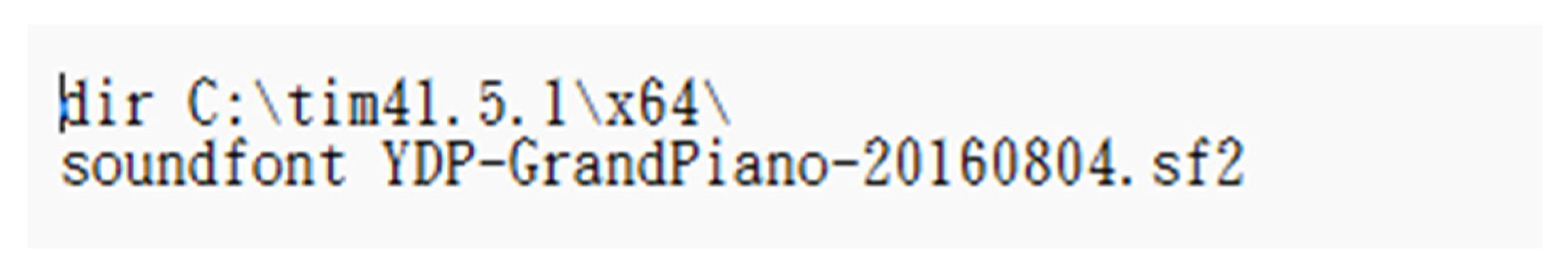
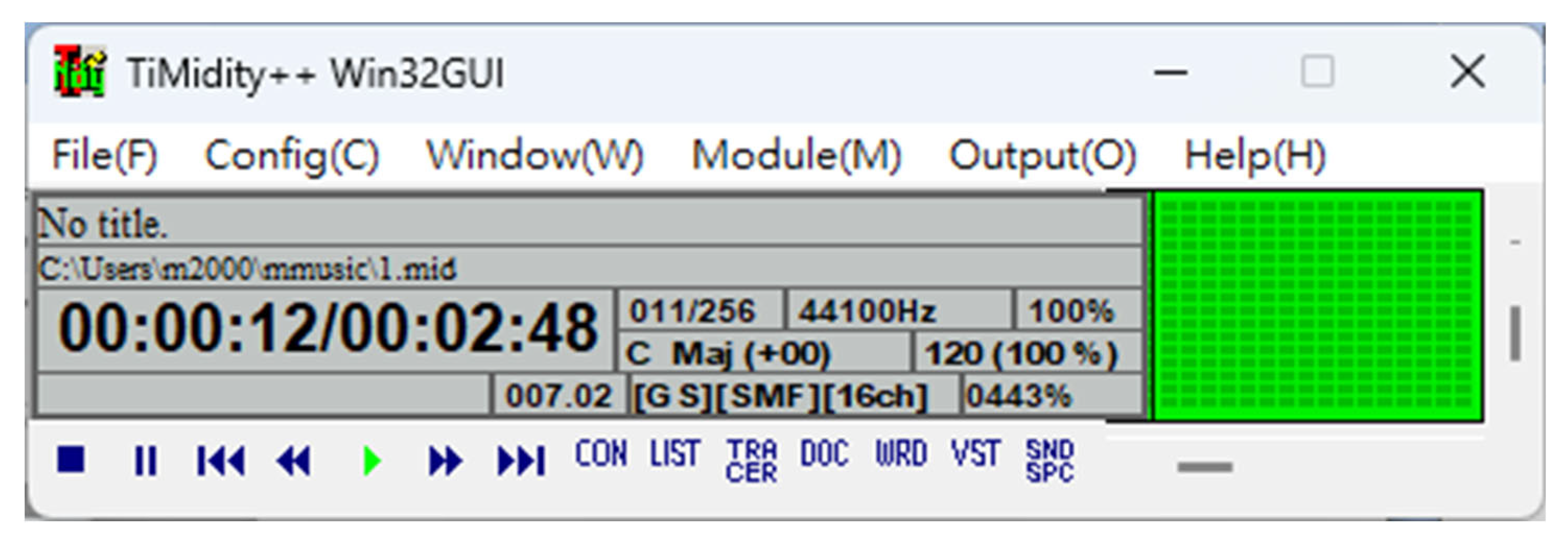
This paper will use Windows 11 as the development environment and install packages such as Anaconda, TensorFlow, Keras, h5py, Timidity [17], FFmpeg [18], and music21 [19]. It will utilize the LSTM network architecture for deep learning and music generation.

2. LSTM Network Design Concept for Music Generation

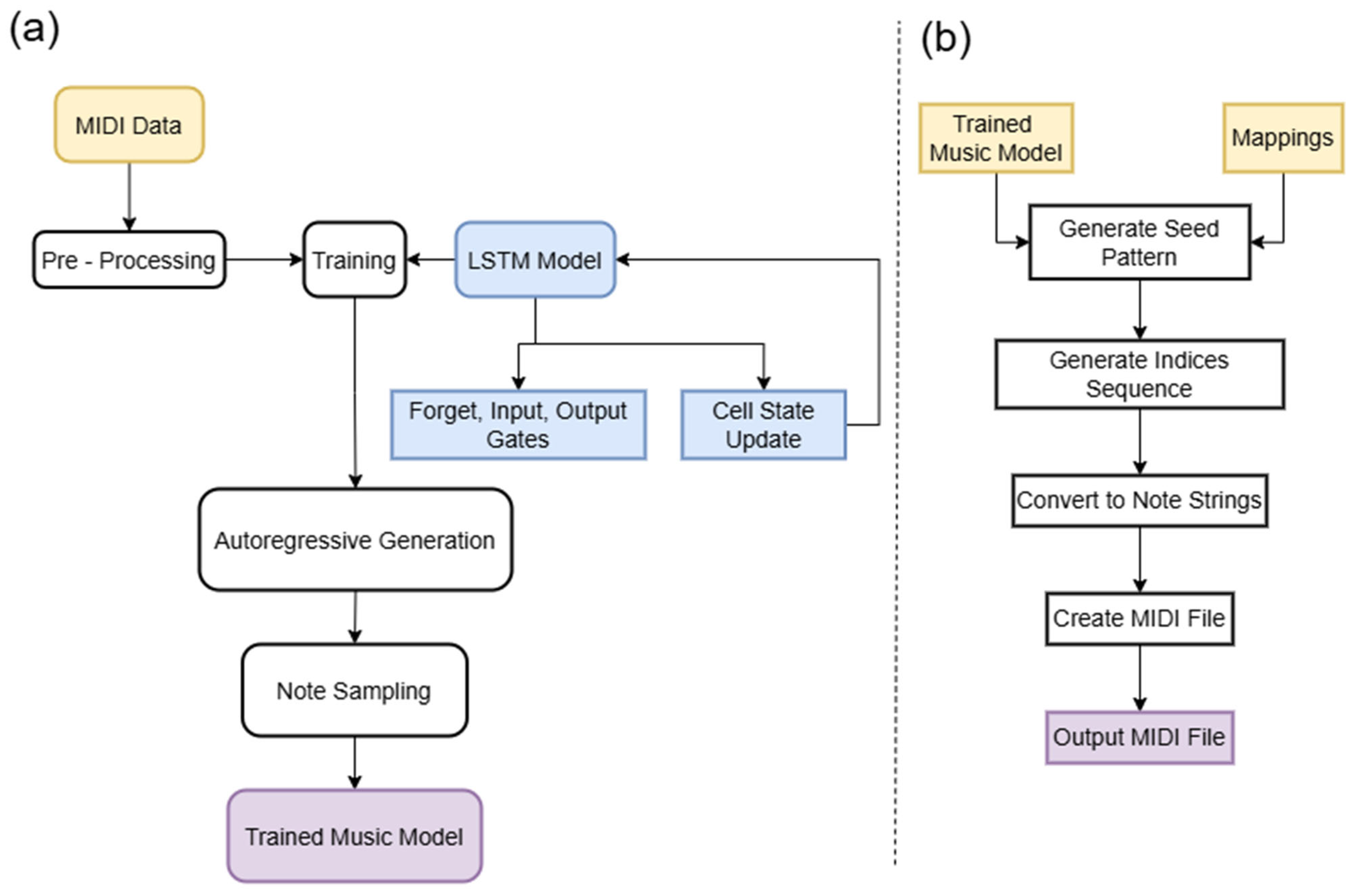
The design concept is shown in Figure 1. The LSTM neural network model is a special type of recurrent neural network (RNN) designed to address the long-term dependency problem in sequence data. To build an LSTM network based on the extracted notes and chords from music21, we can follow these steps to train an hdf5 model:

(1). Data preprocessing: Convert the notes and chords into sequence data suitable for the LSTM model. We can encode each note or chord as a numerical vector representation to input into the LSTM network. Firstly, we collect many Midi music data to perform preprocessing. Please find the details of this work in the Appendix A.

(2). Sequence generation: Based on the preprocessed sequence data, divide it into input sequences and target sequences. For example, define a fixed-length input sequence as the input to the LSTM and the next note or chord as the target output.

(3). Construct the LSTM network model: Use the TensorFlow deep learning framework to build the LSTM model. Define the parameters of the LSTM layer, including the size of the hidden layer, the number of time steps, and other hyperparameters.

(4). Model training: Train the LSTM network using the preprocessed sequence data. Use an appropriate loss function (such as categorical_crossentropy) and optimizer (such as RMSprop) to optimize the model weights.

(5). Model evaluation and auto regressive generation: Use the trained LSTM model to generate new sequences of notes or chords.

(6). Create a dictionary to map numbers to notes and chords, and list the generated notes and chords in order.

After the model is generated, the following process can be used to generate music:

(1). Load Model and Mappings: Load the pre-trained LSTM model and the integer-to-note/chord mapping dictionary from files. Validate the integrity of the model and mappings.

(2). Generate Seed Pattern: Create a random initial sequence of integers (seed) to prime the generation process, ensuring it matches the model’s expected sequence length.

(3). Generate Indices Sequence: Use the LSTM model with temperature sampling to generate a sequence of note/chord indices based on the seed, creating new musical patterns.

(4). Convert to Note Strings: Map the generated integer indices to human-readable note/chord strings using the loaded mapping dictionary.

(5). Create MIDI File: Convert the note/chord strings into a MIDI stream with specified tempo and duration, using the music21 library to handle note/chord objects.

(6). Output MIDI File: Save the generated MIDI stream to a file, with validation to ensure valid notes/chords are present before writing.

An individual LSTM neuron architecture is shown in Figure 2. It consists of an input gate, a forget gate, an output gate, and a cell state. These components interact with musical data in the context of music generation as follows:

Assuming the current time step is $t$, the input is $x(t)$ being a musical representation (such as a one-hot encoded MIDI note or a vectorized musical feature that encapsulates note pitch, duration, and velocity), the previous hidden state is $h(t-1)$, and the previous cell state is $C(t-1)$. In LSTM, $h(t)$ and $C(t)$ represent the current time step’s hidden state and cell state, respectively.

1. Input gate:

$$i(t)=\sigma (W_i\cdot [h(t-1),x(t)]+b_i$$

(1)

where $W_i$ is the input weight matrix; $x(t)$ encodes musical features like the pitch of a note (represented as a MIDI number), its attack velocity, or rhythmic patterns capturing the musical context from the previous time step. The sigmoid function $\sigma$ outputs a value between 0 and 1, and $b_i$ is the bias term. The input gate decides which musical elements from the current time step, such as new melodic contours or dynamic changes, should contribute to updating the cell state.

2. Forget gate:

$$f(t)=\sigma (W_f\cdot [h(t-1),x(t)]+b_f$$

(2)

The forget gate regulates which musical information from the previous cell state, like a recurring chord progression or a motif, should be discarded. $W_f$ is the weight matrix of the forget gate, $\sigma$ is also a sigmoid function, and $b_f$ is the bias term. A value close to 1 indicates retaining the information, while a value near 0 means forgetting it.

3. Candidate state:

$$\tilde{C}(t)=\tanh (W_c\cdot [h(t-1),x(t)]+b_c$$

(3)

The candidate cell state, computed using the tanh function, represents potential new musical content. It is influenced by the current musical input and the previous hidden state. $W_c$ is the weight matrix of the candidate cell state, $b_c$ is the bias term. This candidate state, in conjunction with the input and forget gates, determines how the cell state evolves to incorporate new musical ideas.

4. Update cell state:

$$C(t)=f_t\otimes C(t-1)+i_t\otimes \tilde{C}(t)$$

(4)

where $\otimes$ stands for element-wise multiplication. The updated cell state integrates the retained musical information from the previous time step (controlled by the forget gate) and the newly introduced musical elements (governed by the input gate), thus defining the musical context at the current time step.

5. Output gate:

$$O(t)=\sigma (W_o\cdot [h(t-1),x(t)]+b_o$$

(5)

The output gate dictates which aspects of the current hidden state, such as the harmonic structure or the direction of the melody, should be output. $W_o$ and $b_o$ are the weight matrix and bias term for the output gate, respectively.

6. Hidden state:

$$h(t)=O_t\otimes \tanh (C(t))$$

(6)

The hidden state, calculated based on the output gate and the current cell state, serves as the LSTM’s output for the current time step. It encapsulates the musical knowledge processed so far, which can be used to generate subsequent musical notes.

7. Output layer:

In music generation, $x(t)$ encodes musical information (e.g., a specific note or a short musical phrase). The objective is to predict the probability distribution of the next musical note ${\widehat{y}}_t$:

$${\widehat{y}}_t=Softmax(W_h{h}_t+b_h)$$

(7)

where ${\widehat{y}}_t\in R^N$, N represents the number of possible musical notes (e.g., 128 MIDI notes). This output can be used to sample the next note in a generated musical sequence, taking into account the learned musical patterns and context within the LSTM. In the realm of music generation, N denotes the cardinality of the musical note space, typically corresponding to 128 MIDI notes which span the full chromatic range from the lowest to the highest audible pitches.

In the music generation task, the input $x(t)$ is usually the encoding of notes (such as one-hot encoding of MIDI numbers or embedding vectors), and the goal is to predict the probability distribution of the next note $\widehat{y}(t)$ based on the historical note sequence. The following takes single pitch sequence prediction (such as a MIDI number sequence) as an example for illustration: 1. For the input Layer: Convert notes into numerical values (such as MIDI number $p(t)$, and map them into dense vectors $e(t)$ through the Embedding Layer, i.e., $x(t)=e(t)$. 2. For the output Layer: Use the Softmax activation function to output the probability distribution of the next note, which is as Equation (7).

Let the training data be $\left\{\begin{array}{cccc}[x(1),y(1)]& [x(2),y(2)]& \cdots & [x(T),y(T)]\end{array}\right\}$, where $y(t)$ is the true note number (one-hot encoding) at time $t$. The loss function is cross-entropy:

$$E=-{\displaystyle \frac{1}{T}}{\displaystyle \sum _{t=1}^T{\displaystyle \sum _{i=1}^N{y}_i(t)}}\log {\widehat{y}}_i(t)$$

(8)

where N is the total number of note categories (such as the number corresponding to the MIDI number range). The training objective is to optimize the parameters $\left[\begin{array}{cccccccccc}{W}_f& W_i& W_c& W_o& W_h& b_f& b_i& b_c& b_o& b_h\end{array}\right]$ of the LSTM through backpropagation through time (BPTT) to minimize the loss function.

After training, the LSTM generates music through an autoregressive approach; the learning process of LSTM for music generation essentially models the temporal dependencies of the note sequence through the mathematical operations of the gating mechanism, and optimizes the parameters through backpropagation to fit the probability distribution of the training data. The core of its mathematical derivation lies in the dynamic adjustment of the gating signals and the long-term transfer of the cell state, ultimately achieving the learning of patterns from historical data and the generation of new musical sequences.

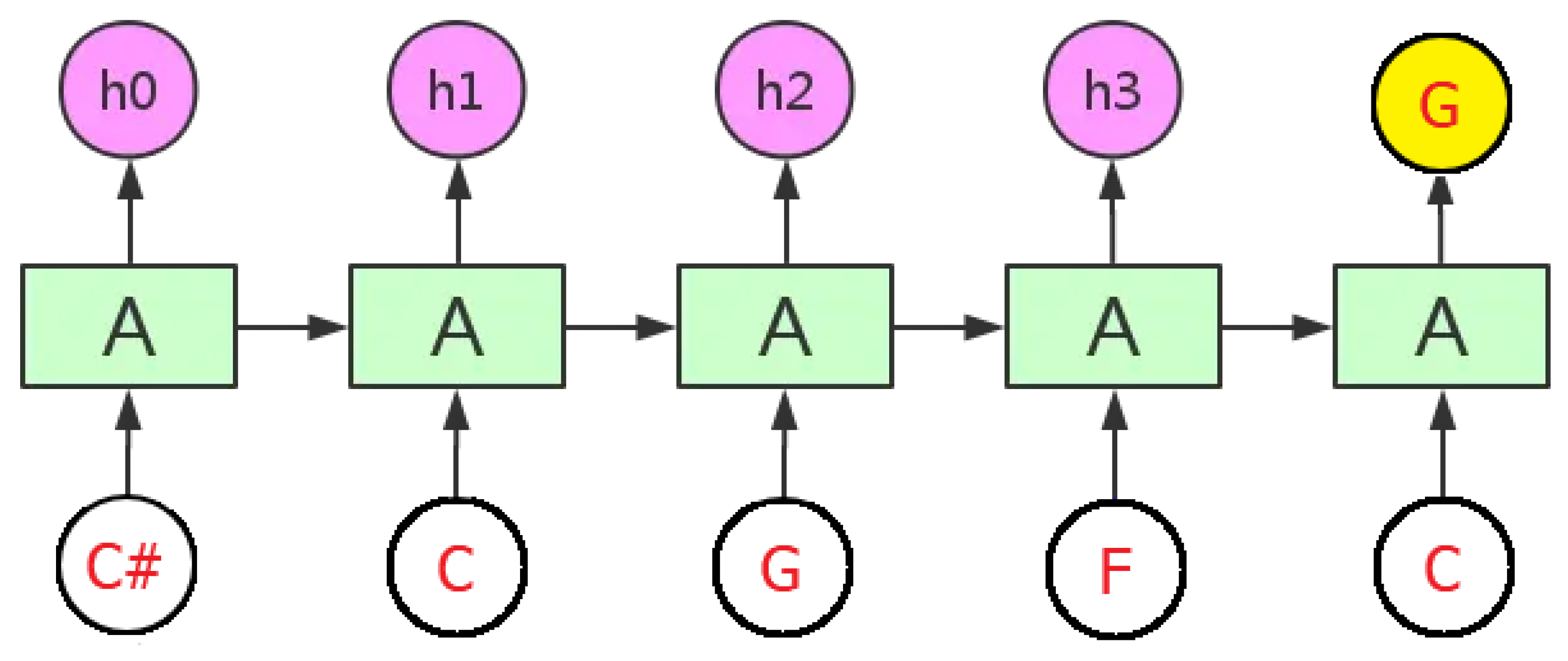
If we consider an individual neuron as A, the continuous action of LSTM in music generation is shown in Figure 3. After remembering the previous segment, when receiving the note C next, the output will be G. In short, the design of LSTM is to control and filter the flow of information in the cell state. By controlling the forget gate, input gate, and output gate, LSTM can capture long-term dependencies in sequence data and effectively handle the issues of vanishing or exploding gradients. This makes LSTM performwell in tasks that require long-term memory, such as language modeling, machine translation, speech recognition, and music generation.

To optimize the effect of generated music and distinguish between samples and generated music using different line styles during visualization, we can make the following improvements:

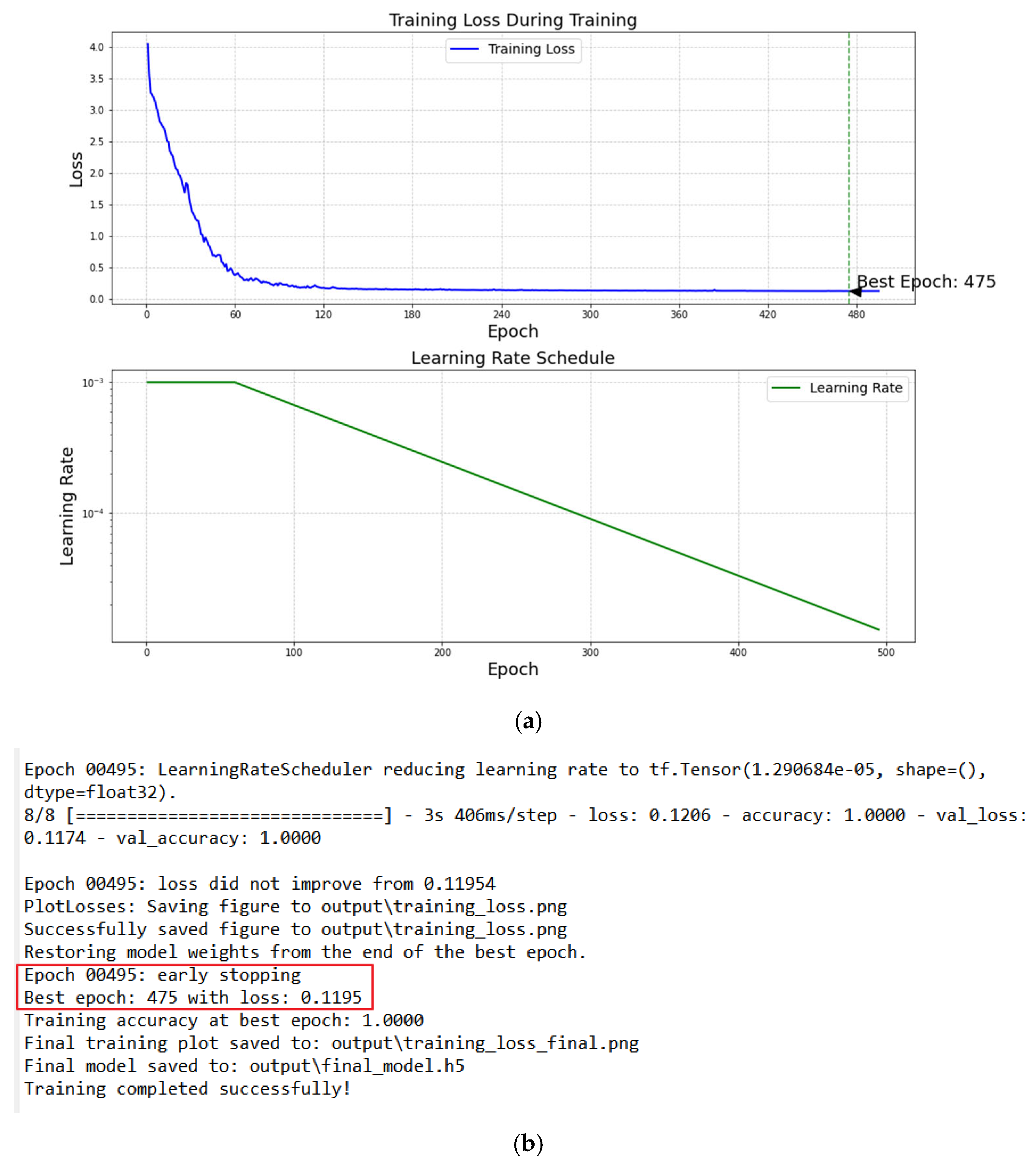
Increase training data and training epochs: More data and longer training can enable the model to learn more diverse patterns. While increasing training data and epochs may initially improve performance, excessive epochs can lead to overfitting. To address this, I have included anexplanationof early stopping as a critical mitigation strategy in Section 4.

Optimize the generation logic: When generating music, introduce some randomness to avoid always choosing the note with the highest probability.

Visualization optimization: Draw samples with dashed lines and generated music with solid lines.

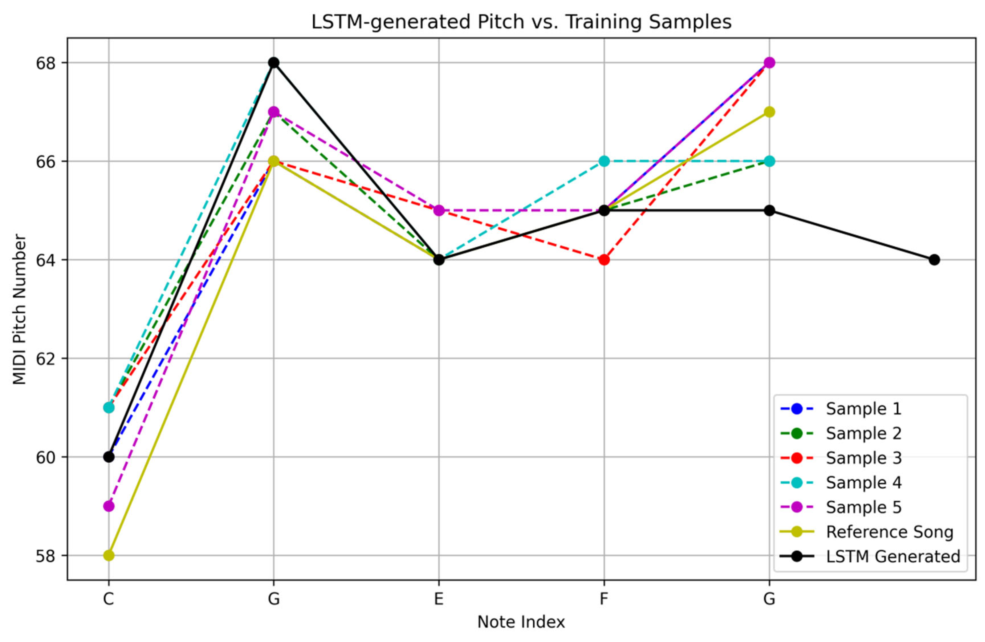
Using five randomly generated simple song samples with pitch sequences of C, G, E, F, and G, process them using Python 3.5, and plot the pitch and velocity graphs. This defines the pitch sequences of [‘C’, ‘G’, ‘E’, ‘F’, ‘G’]. After running the code, we will see five sets of pitch and velocity graphs, and five MIDI files will be generated in the current directory. The pitch diagram is shown in Figure 4.

Figure 4 is designed to visualize the performance of the LSTM model in generating musical sequences, specifically focusing on pitch distribution and continuity. The y-axis represents pitch numbers (e.g., MIDI note values) to illustrate the melodic contour generated by the model at different time steps (x-axis). While the figure primarily serves as a qualitative visualization of pitch patterns, we can derive quantitative insights from it indirectly. For example:

1. Pitch Range Consistency: By observing the spread of pitch numbers, we can assess whether the model generates notes within the expected musical range (e.g., typical piano register, 21–108 in MIDI).

2. Melodic Coherence: The smoothness of pitch transitions (e.g., stepwise motion vs. large leaps) reflects the model’s ability to learn melodic rules from the training data. Sudden, unrealistic leaps might indicate underfitting, while repetitive patterns could suggest overfitting.

3. Distribution Match: Although not a direct quantitative metric, comparing the pitch density in the figure to the training data’s pitch distribution (e.g., via a histogram) can hint at how well the model captures the statistical properties of real music.

3. Implementation

For implementation, TensorFlow was used to develop the program. The algorithms for generating code are shown below Algorithms 1 and 2:

Algorithm 1: Neural Network Training with Early Stopping

Input: Training data D, seq. length L, batch size B, max epochs E, patience P. Output: Trained model weights W saved to HDF5. 1: Load D, create pitch mappings P and I 2: Prepare sequences X, Y from D 3: Split X, Y into training/validation sets 4: Build LSTM model with BN, Dropout, L2 regularization 5: Compile model with Adam optimizer and cross-entropy loss 6: Initialize best_loss← 100, patience_counter← 0 7: for epoch = 1 to E do 8:    Train model for one epoch 9:    Compute validation loss L_val 10:  if L_val<best_loss then 11:    best_loss←L_val 12:    Save weights W 13:    patience_counter← 0 14:  else 15:    patience_counter←patience_counter + 1 16:  end if 17:  if patience_counter ≥ P then 18:    Break training loop (Early Stopping) 19:  end if 20: end for 21: Load best weights W 22: Save final model and mappings

Algorithm 2: Harmonically Constrained Music Generation

Input: HDF5 model path, training data, sequence length, generation length, chord progression, temperature factor. Output: MIDI melody file 1: Load training data and create pitch mappings 2: Build neural network model architecture 3: Load pre-trained weights from HDF5 file 4: Initialize input sequence from training data 5: for each note in generation length do 6:    Predict pitch probabilities using model 7:    Apply harmonic constraints: 8:       Increase chord tones by 300% 9:       Increase scale tones by 150% 10:  Reduce non-harmonic tones to 10% 11:  Normalize probabilities to sum to 1 12:  Apply temperature scaling to probabilities 13:  Sample next pitch index from adjusted probabilities 14:  Add sampled pitch to melody and update input sequence 15: end for 16: Structure melody into AABA form: 17:  Split into sections A (120 notes) and B (60 notes) 18:  Transpose section B by minor third interval 19:  Recombine as A + A + B + A 20: Create MIDI file with melody and harmonic accompaniment

The program architecture is shown in Figure 5. Training was conducted for more than 500 epochs. The CPU used was Intel i7-10700, and the GPU was NVIDIA GeforceGT-1030. The dropout rate for LSTM layers was determined through a combination of domain knowledge, grid search, and validation performance monitoring. I began with dropout rates commonly used in sequence models (0.1–0.3), as higher values risk disrupting the temporal dependency learning critical for music generation. I performed a systematic grid search over candidate values (0.1, 0.2, 0.3) using a validation set of held-out musical sequences. After 475 epochs, the loss reached 0.1195, as depicted in Figure 6. The output file will be generated as a MIDI format by using the “FFmpeg” tool.

4. Comparison and Analysis

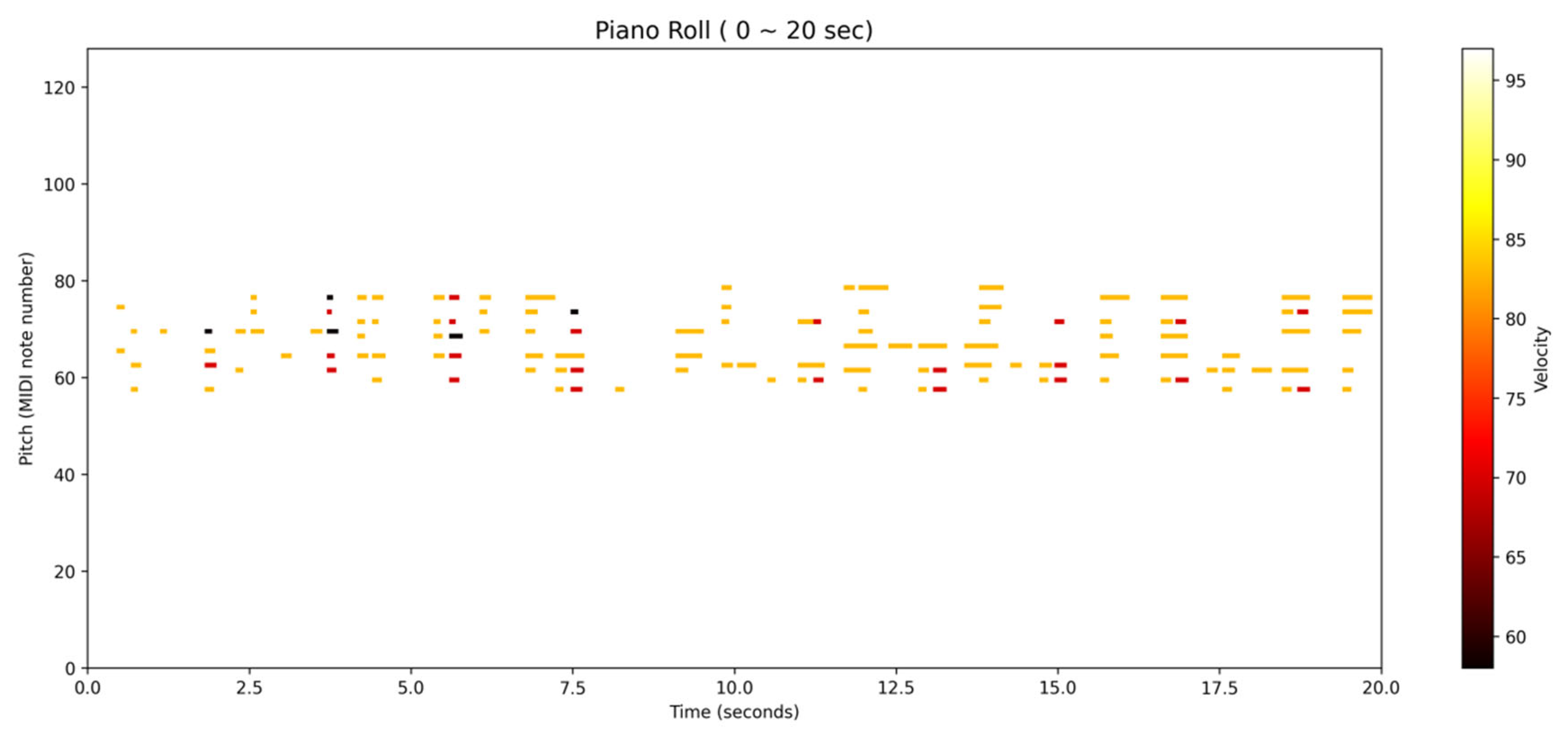
If we compare a piece of music (the original duration of the music is 2 min and 20 s), I capture 20 s of it for illustration. It can show the characteristics of the original music’s pitch and velocity. The Midi format diagram is shown in Figure 7. Then, we can get the characteristic diagram shown in Figure 8.

In a tonal composition, the model’s prediction will be influenced by the established key signature, with notes within the key having higher probabilities of being selected. In terms of technical implementation, the Softmax function normalizes the raw output scores from the neural network into probabilities, enabling a probabilistic sampling approach. Techniques like temperature-adjusted sampling can be applied here. A lower temperature value will lead to more conservative, “safe” note selections, adhering closely to learned musical patterns and common progressions, while a higher temperature encourages more creative and exploratory outputs, potentially introducing novel melodic or harmonic turns. This way, the model not only generates new musical sequences but also balances between adhering to established musical conventions and exploring new musical territories, leveraging the learned context and patterns within the LSTM architecture.

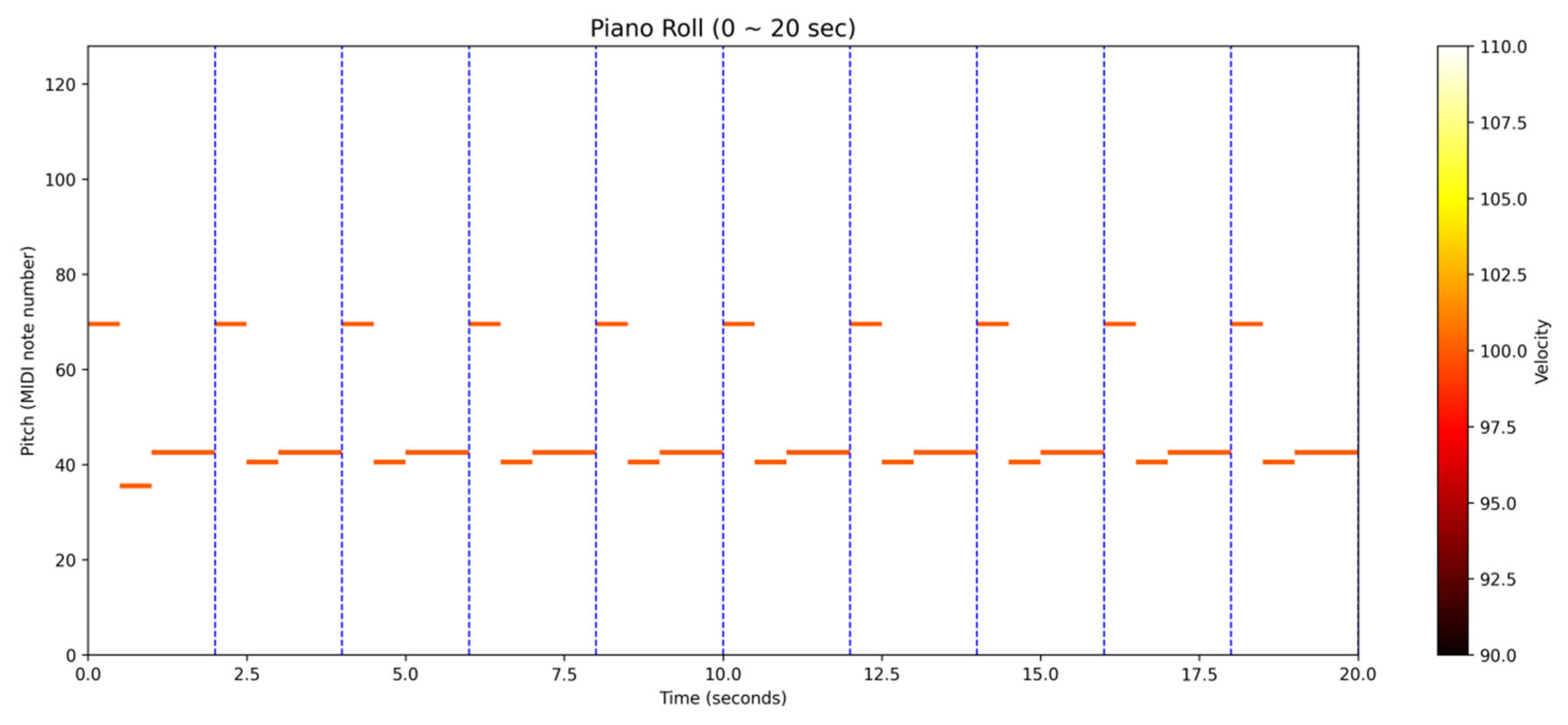
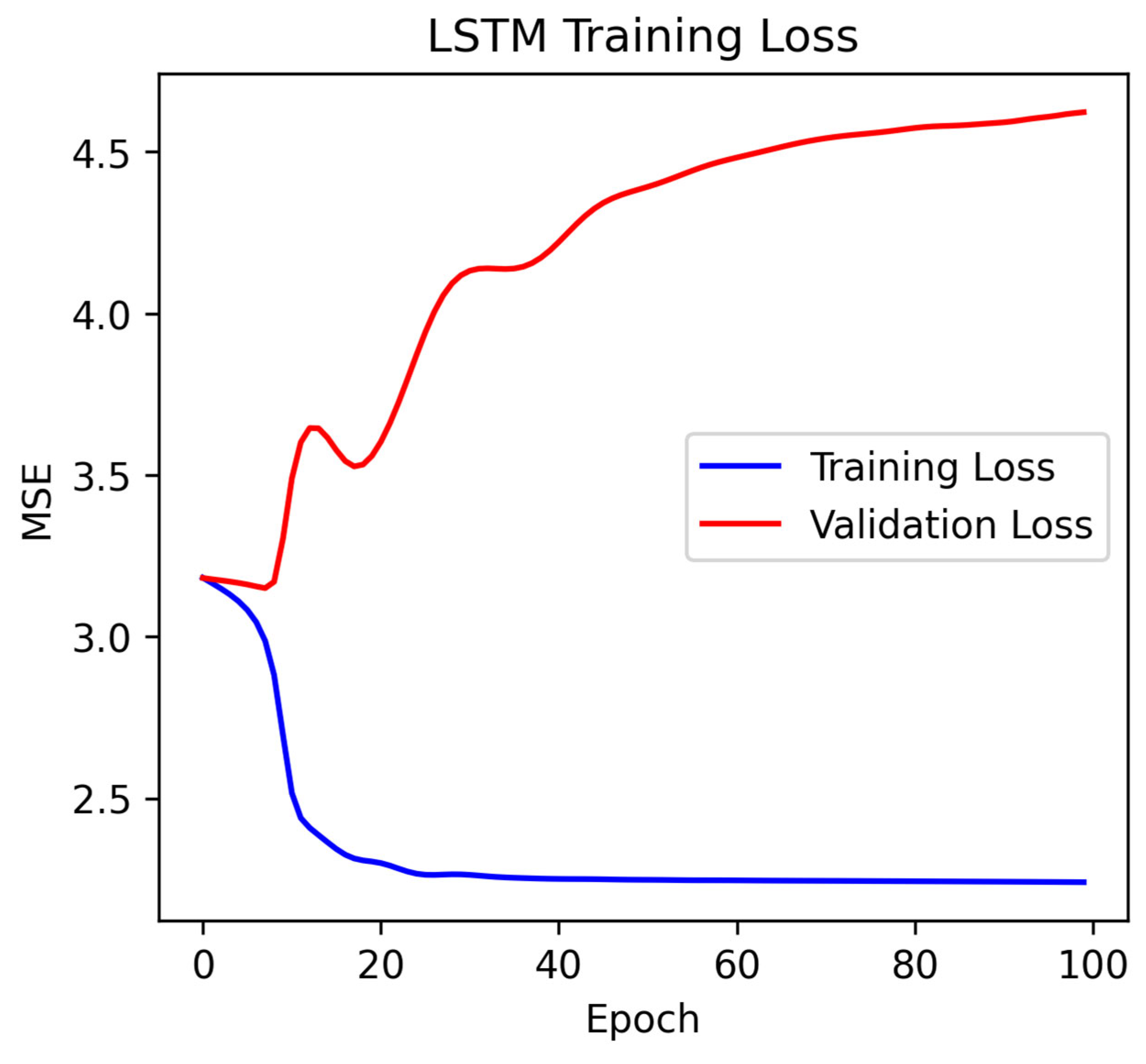
If the information we extract is only pitch but not duration, then the LSTM will have difficulty learning. In other words, it has too few notes and it is useless to increase the epoch, so the learning effect will be poor such as in Figure 9.

In order to improve our shortcomings, we set and design the following strategies:

1. Data preprocessing:

Normalization: Use the parameter “MinMaxScaler” to ensure that the input features are at the same scale to avoid vanishing gradients.

Reasonable window size: Set the parameter “window_size = 30” to balance the context information and the amount of computation.

2. Model architecture optimization:

We use bidirectional LSTM to capture contextual dependencies and improve sequence modeling capabilities. The discrete notes (0–127) are mapped to a low-dimensional continuous space in the Embedding layer parameter “Embedding”, reducing the input dimensionality. The parameter “LayerNormalization” should be declared, which can speed up training convergence and alleviate gradient instability.

3. Training strategy:

Learning rate scheduling: Use cosine annealing to dynamically adjust the learning rate to avoid falling into the local optimum. The parameter “Early Stopping” should be set so that the validation loss can be monitored to prevent overfitting and terminate the training early. Use small batch training, and set the parameter “Batch Size” to 128 to balance memory usage and gradient update stability.

4. Regularization

This uses L2 regularization: set the parameter “kernel_regularizer” to 12 to reduce the risk of overfitting.

Validation split: Setting the parameter “validation_split” to 0.2 can monitor the generalization ability of the model in real time.

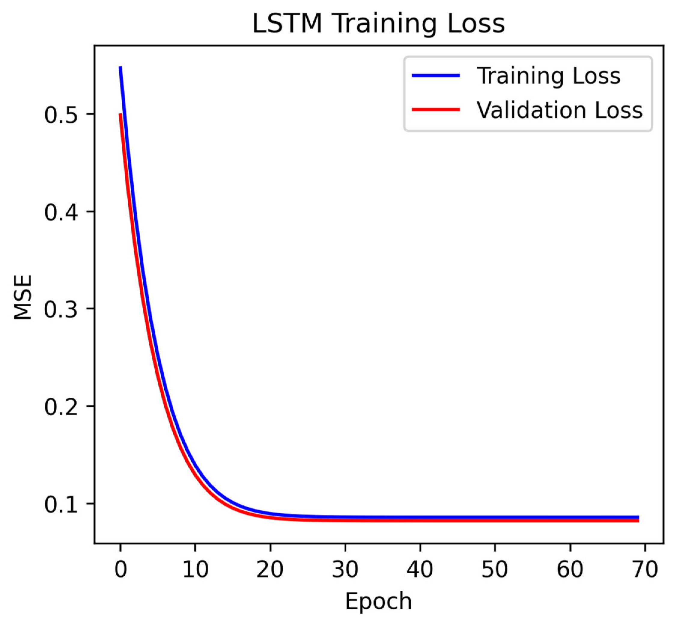
5. Real data replacement: Use MIDI datasets (such as MAESTRO) to replace random simulated data and extract features such as pitch, rhythm, and dynamics. Upgrade models; use Transformer architecture (such as MusicGPT [20]) to handle long sequence dependencies, or use GANs to generate adversarial training to improve music authenticity. While MusicGPT is not explicitly labeled as the “current SOTA” in all music generation tasks (as the field evolves rapidly), it represents a significant advancement intext-to-music generation and has been referenced in recent literature for its ability to produce high-quality, semantically aligned outputs. The results are shown in Figure 10 and Figure 11.

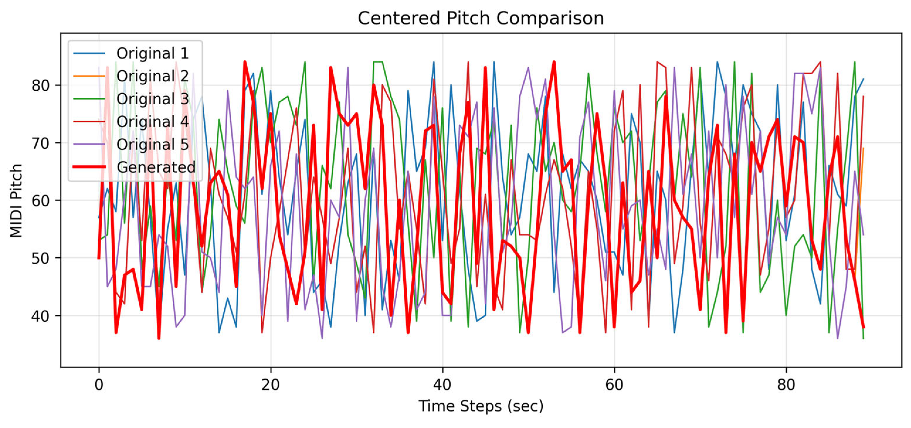
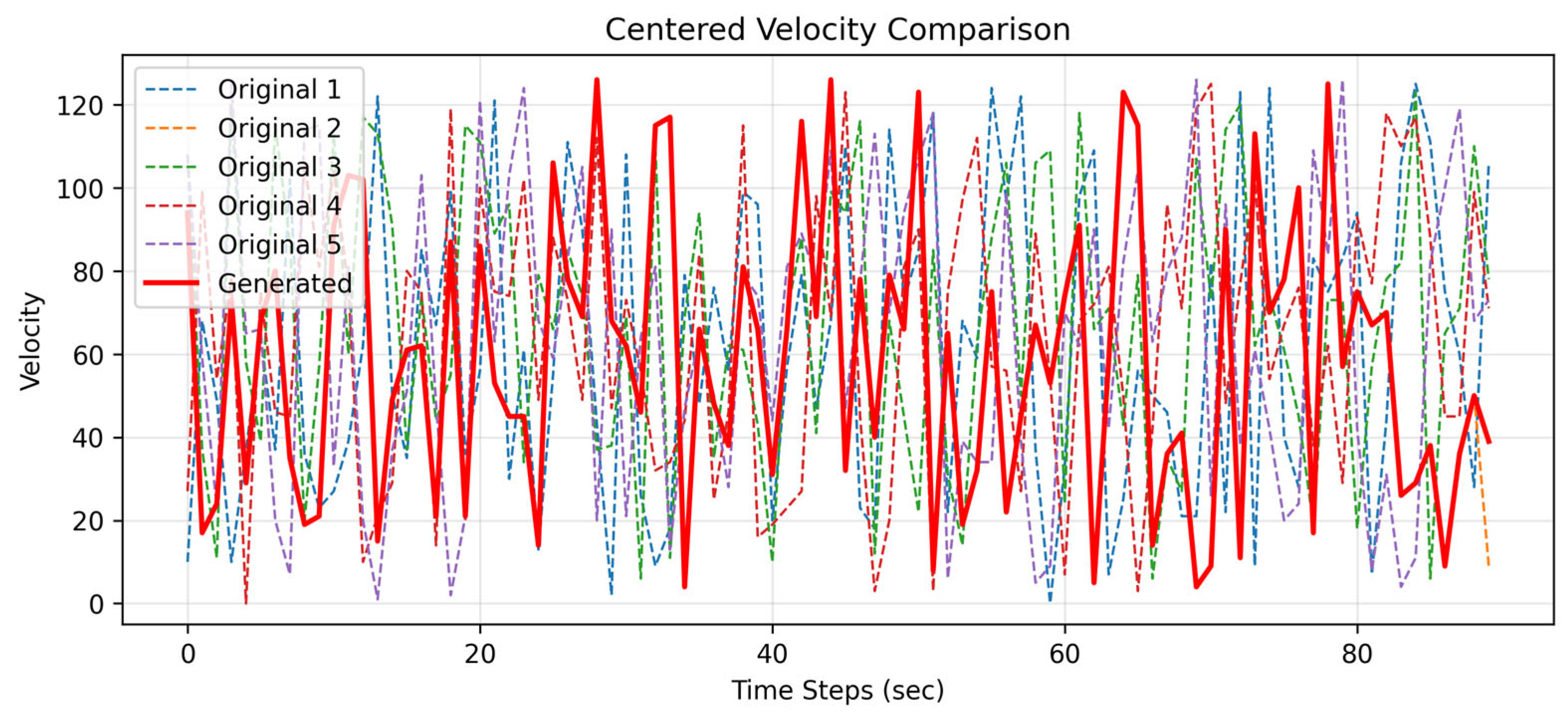
I selected the first 90 s of 5 original songs in the same style for comparison. After training with our LSTM architecture, we generated a piece of music with pitch and velocity features. The comparison results are shown in Figure 12 and Figure 13. We found that all 90 s segments were trainable, yielding corresponding generated results that met our expectations and demonstrated excellent performance.

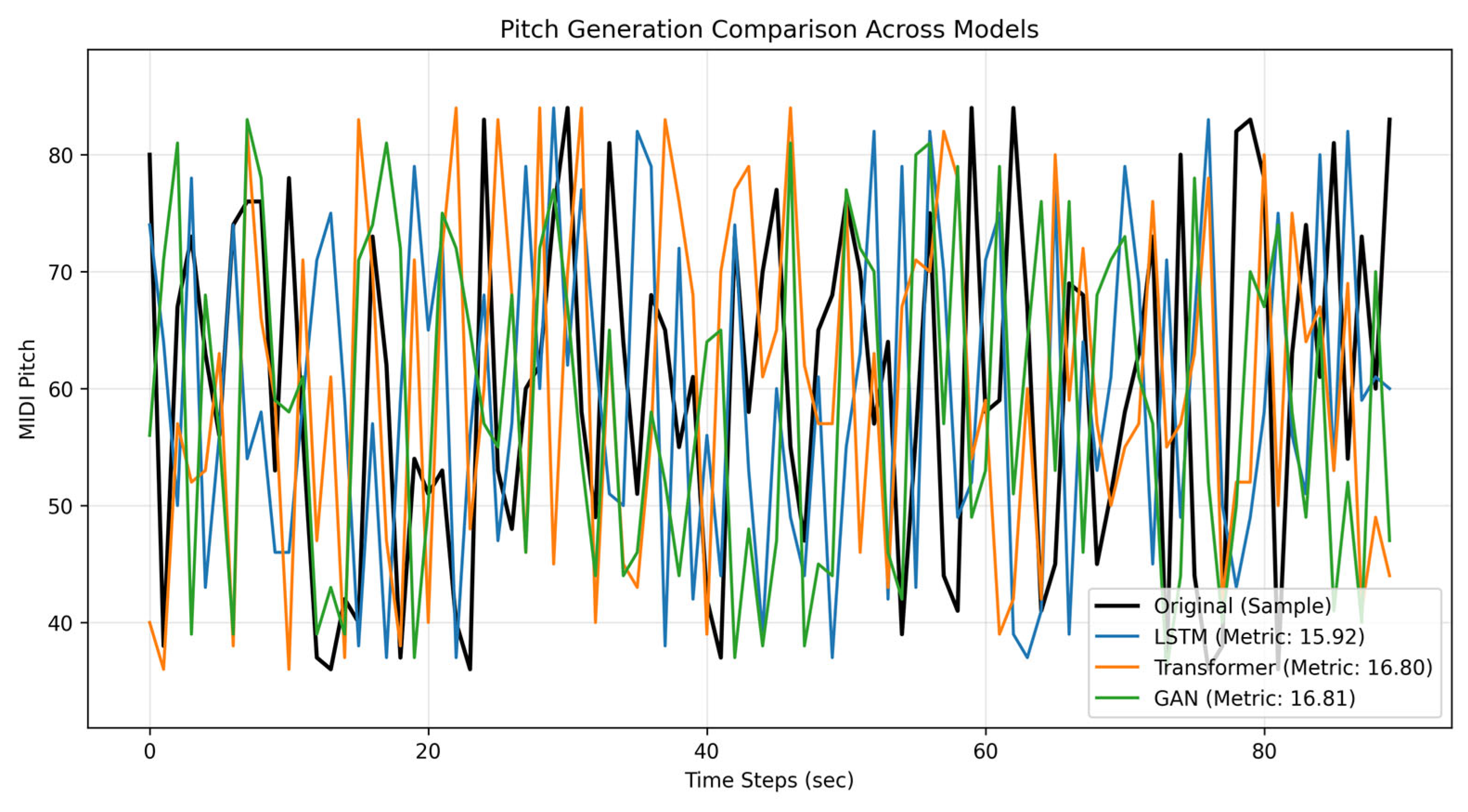
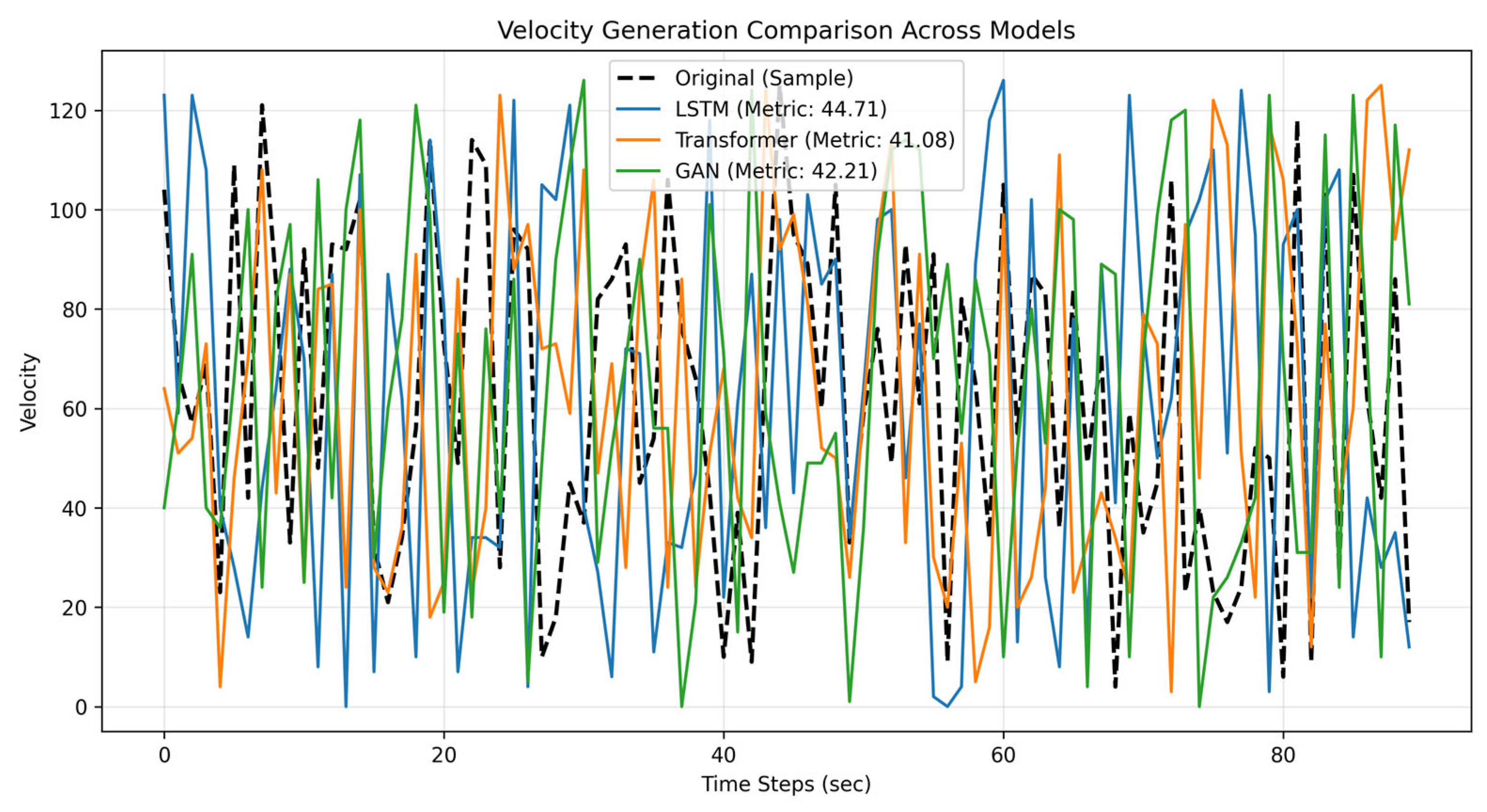
The comparison plots shown in Figure 14 and Figure 15 evaluate three models—LSTM, Transformer, and GAN—for music generation by analyzing their ability to replicate real MIDI pitch and velocity patterns. Key metrics include the “Average Distance to Original” data (lower is better: the metric calculatesthe mean absolute difference between generated values and real data, measuring how closely the model mimics the original patterns), and visual alignment with real sequences (black lines). LSTM excels in sequential coherence, Transformer handles long-range dependencies effectively, and GAN prioritizes diversity. Use

Table 2. A comparison table of LSTM, Transformer, and GAN.

Model	Average Pitch Distance	Velocity Average Distance	Features
LSTM	15.92	44.71	Strong sequential modeling capabilities and high generation coherence
Transformer	16.80	41.08	Global attention mechanism, effectively handles long-sequence dependencies
GAN	16.81	42.21	Strong diversified generation ability and higher creativity

to compare quantitative performance and the plots to assess qualitative trends (e.g., smoothness, variability). For practical applications, choose LSTM/Transformer for high fidelity or GAN for creative diversity.

5. Conclusions

Although the technology of music generation is already very mature, there are still many technical details to pay attention to when generating a piece of music. In the Windows environment, we can use open-source projects such as TensorFlow, music21, FFmpeg, and abundant high-quality music training data to achieve music generation based on the LSTM deep learning architecture. However, we need to pay attention to the setting of many parameters, which requires an understanding of the entire music generation architecture. These architectures can capture the temporal dependencies of musical sequences and produce musical compositions with considerable structure and creativity. Through implementation, it is demonstrated that LSTM can effectively achieve the production of perfect, original, and subjectively attractive short- and medium-term musical compositions.