1. Introduction
In the rapidly evolving field of quantum computing, as of now, no quantum computer possess the capability to fundamentally disrupt the computational landscape. However, the remarkable progress witnessed in recent years suggests that such a transformative shift may be imminent. Over the past few months, leading organizations and research teams have achieved groundbreaking milestones, significantly advancing the development of quantum technologies and their potential applications. Building on the success of the 127-qubit Eagle processor [
1] and the 433-qubit Osprey processor [
2], IBM has made significant strides with the introduction of the 1121-qubit Condor processor [
3], and the cutting-edge R2 Heron, recognized as IBM’s most powerful quantum processor to date [
4]. These advancements enhance the computational capacity that is required for complex quantum algorithms, including those used in function classification. Google has recently demonstrated the superior performance of quantum computers over the most advanced classical supercomputers, as documented in [
5,
6]. These breakthroughs underscore the potential of quantum systems to tackle computationally intensive tasks, such as the classification of Boolean and generalized functions, with unprecedented efficiency. Microsoft has unveiled the revolutionary Majorana 1 quantum chip, a significant development poised to redefine quantum computing capabilities [
7,
8,
9]. This innovation promises to enhance the scalability of quantum systems, supporting demanding applications in cryptography and quantum classification. In the realm of quantum annealing, D-Wave has achieved a notable success by using a quantum processor to solve a scientifically significant problem faster than classical computers, as reported in [
10,
11]. This milestone highlights the potential of quantum annealers to address optimization problems, which can also be useful for classification tasks. At the same time, other research teams have reported significant breakthroughs. Although this report is far from exhaustive, we believe that some of the most significant recent advancements are as follows. The state-of-the-art Zuchongzhi 3.0 quantum processor, featuring 105 qubits, represents a significant technological step in quantum hardware development [
12,
13]. This processor enhances the computational power available for quantum algorithms, including those leveraging algorithms for function analysis. Beyond individual processors, recent advancements include novel design concepts [
14,
15] and innovative hardware solutions [
16,
17]. A particularly noteworthy development is the demonstration of distributed quantum computing, where researchers successfully connected two separate quantum processors via a photonic network interface, creating a unified, fully integrated quantum computer [
18,
19]. This breakthrough in distributed quantum computing opens new possibilities for scalable quantum systems, which could significantly enhance the implementation of quantum classification algorithms.
This research introduces a novel and innovative perspective on the quantum classification of Boolean functions, redefining the approach to this significant challenge within the realm of quantum computing. Our study focuses on the capabilities of quantum classification algorithms, which can achieve a classification probability of
for functions that adhere to specific, well-defined characteristics—referred to as the “promised class”. However, the central objective of this work is to investigate the extent to which meaningful insights can be derived when the input function deviates from this promised class, presenting a scenario where classification becomes inherently more complex. To make these technical concepts more accessible and engaging, we present our quantum classification algorithm in the form of a game featuring the well-known characters Alice and Bob. By leveraging the entertaining and intuitive nature of games, we aim to facilitate a clearer understanding of the underlying quantum principles for a broader audience. Since the seminal works of Meyer [
20] and Eisert et al. [
21], quantum games have gained significant traction in the research community, largely due to the demonstrated superiority of quantum strategies over their classical counterparts in various scenarios. A prime example is the quantum version of the Prisoners’ Dilemma [
21], which serves as a compelling case study and has inspired the development of numerous abstract quantum games, as explored in the recent literature [
22]. Beyond their entertainment value, quantum games have proven to be powerful tools for addressing serious computational challenges, including the design of cryptographic protocols, as evidenced by foundational work in quantum cryptography [
23] and recent advancements [
24]. Furthermore, the principles of quantum games have been extended to transform classical systems into quantum frameworks, including applications in political and social systems, highlighting their versatility and potential impact across diverse domains.
1.1. Related Work
The field of quantum classification has seen remarkable progress since the introduction of the seminal Deutsch–Jozsa algorithm [
25], which laid the foundation for leveraging quantum advantages in function classification. This pioneering work has inspired a series of sophisticated contributions that have expanded the scope and capabilities of quantum classification algorithms. For instance, Cleve et al. [
26] explored a multidimensional generalization of the Deutsch–Jozsa problem, which was further refined by Chi et al. [
27] through an in-depth analysis of evenly distributed and balanced Boolean functions. Subsequent advancements by Holmes et al. [
28] adapted the Deutsch–Jozsa algorithm to classify balanced functions within finite Abelian subgroups, broadening its applicability. Another notable generalization was proposed by Ballhysa et al. [
29], while Qiu et al. [
30] extended the Deutsch–Jozsa framework and introduced an optimized algorithm for enhanced performance. More recently, Ossorio-Castillo et al. [
31] presented an innovative generalization of the Deutsch–Jozsa algorithm, pushing the boundaries of quantum classification. Practical applications of this algorithm have also been explored in works such as [
32,
33], demonstrating its versatility in real-world scenarios. Furthermore, significant efforts toward developing distributed versions of the Deutsch–Jozsa algorithm have been documented in [
34,
35], highlighting the potential for scalable quantum classification systems. In a related vein, Nagata et al. [
36] extended Deutsch’s original algorithm to binary Boolean functions, enriching the theoretical framework for quantum classification. The broader literature on Quantum Learning and Quantum Machine Learning has also contributed significantly to this domain, with key studies such as [
37,
38,
39,
40,
41,
42] focusing on oracular algorithms for computing and classifying Boolean functions. These works predominantly emphasize the distinction between constant and balanced functions, where a balanced function is defined as one whose domain elements yielding output 0 are equal in number to those yielding output 1. In contrast, a recent study by Andronikos et al. [
43] shifts the focus to imbalanced Boolean functions, introducing the novel BFPQC (Boolean Function Pattern Quantum Classifier) algorithm, which is designed to classify a diverse class of imbalanced functions exhibiting specific behavioral patterns, leveraging pattern-based hierarchies.
Quantum classification algorithms are typically guaranteed to succeed only when the input function satisfies certain well-defined properties, forming what is commonly referred to as a “promise problem”. In essence, if the input function belongs to a rigorously specified category—such as the promised class defined by the pattern bases in the BFPQC framework—the algorithm will produce accurate results. However, if the input function deviates from these properties, the algorithm’s performance is not guaranteed, most often leading to erroneous outcomes. The literature consistently emphasizes this limitation, with authors meticulously outlining the precise conditions under which their algorithms are applicable [
25,
26,
30]. To the best of our knowledge, the vast majority of prior work has not systematically investigated the behavior of quantum classification algorithms when the input function lies outside the promised class, leaving a critical gap in understanding their robustness and applicability.
Contribution. Quantum classification algorithms represent a promising approach to categorizing functions that adhere to specific structural properties, achieving a perfect classification probability of when these conditions are met, a concept widely recognized in the literature as a “promise problem”. The “promised class” encapsulates the rigorously defined set of functions that satisfy these properties, ensuring the algorithm’s optimal and reliable performance. In this study, we establish a precise and formal definition of the promised class in Definition 13. To eliminate any potential ambiguity, we emphasize that the algorithm’s effectiveness is contingent upon the input function belonging to this promised class; when the function deviates from this class, the algorithm is not expected to yield accurate results, as the absence of the required properties undermines its reliability. From an implementation standpoint, these algorithms leverage a quantum oracle that efficiently evaluates the input function, a pivotal component that harnesses the quantum advantage in classification tasks.
The primary objective of this research is to address a significant gap in the literature by investigating whether meaningful insights can be extracted when the input function lies outside the promised class, a challenging scenario that tests the robustness of quantum classification algorithms. To ensure a rigorous and productive investigation, we adopt a well-defined framework based on specific assumptions. Our analysis centers on the BFPQC algorithm, introduced in [
43], which is designed to classify all Boolean functions within the promised class with optimal accuracy and a probability of
using a single oracular query. In this work, we extend our exploration to examine the behavior of the BFPQC algorithm when applied to functions that, while not members of the promised class, are sufficiently close to its elements, as formalized in Definition 19. This represents a noteworthy advancement, as, to the best of our knowledge, this study is the first to provide rigorous evidence that quantum classification algorithms can yield valuable insights into the structure and behavioral patterns of functions outside the promised class, offering a novel perspective on their classification and potential applications.
A key innovation of this work is the introduction of a novel concept of “nearness” between Boolean functions, which quantifies proximity to the promised class through a carefully defined distance metric. By applying this concept, we demonstrate that the BFPQC algorithm can extract significant information about the behavioral patterns of functions that are close to the promised class, thereby expanding the algorithm’s utility beyond its original scope. Within our framework, the notion of left and right cluster proximity serves as a robust criterion for assessing nearness, providing a structured and mathematically rigorous approach to evaluate how closely an unknown function aligns with the promised class. This concept of “nearness” is not only a novel contribution to the literature but also appears to offer distinct advantages over alternative distance metrics. For example, the Hamming distance, which counts the number of inputs where two functions differ, is a straightforward and intuitive metric but is limited in the quantum context due to the projective nature of quantum states, which prioritizes phase and amplitude differences over simple value discrepancies. Our analysis strongly suggests that imposing a distance-based constraint is critical for any quantum classification algorithm to yield useful insights when dealing with functions outside the promised class.
1.2. Organization
This article is structured in the following way.
Section 1 introduces the topic and includes references to relevant literature.
Section 2 offers a brief overview of key concepts, which serves as a basis for grasping the technical details.
Section 3 and
Section 4 rigorously define the promised class itself, and what we perceive as Boolean functions being outside the promised class, but still close enough to it.
Section 5 provides an in-depth analysis of the information that Alice can infer about the behavioral pattern of the unknown function. Finally, the paper wraps up with a summary and a discussion of the algorithm’s nuances in
Section 6.
2. Background Concepts
To begin, we will establish the notation and terminology that will be utilized throughout this article.
is the binary set .
is a sequence of n bits that makes up a bit vector of length n. zero and one are two special bit vectors, represented by and , respectively, where all the bits are zero and one: and .
For clarity, we write in boldface when referring to a bit vector . For convenience, is frequently viewed as the binary representation of the integer b.
It is also useful to think of each bit vector as the binary correspondence to one of the basis kets that constitute the computational basis of the -dimensional Hilbert space.
Definition 1 (Boolean Functions)
. A Boolean function f is a function from to , .
Example 1 (Boolean Functions)
. We give now two examples of Boolean functions. The binary Boolean function f and the ternary Boolean function g are defined as shown below: The above functions assume the values listed in Table 1. In this work, when studying a system consisting of
n qubits, we shall often refer to following signature state
as the perfect superposition state. This state is of particular importance because it is the starting point of most quantum algorithms. In modern quantum computers it is easily prepared by acting with the
n-fold Hadamard transform on the initial state
. Two other important states are the
and
states, which are defined as
Example 2 (Perfect Superposition State)
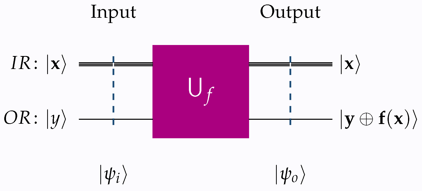
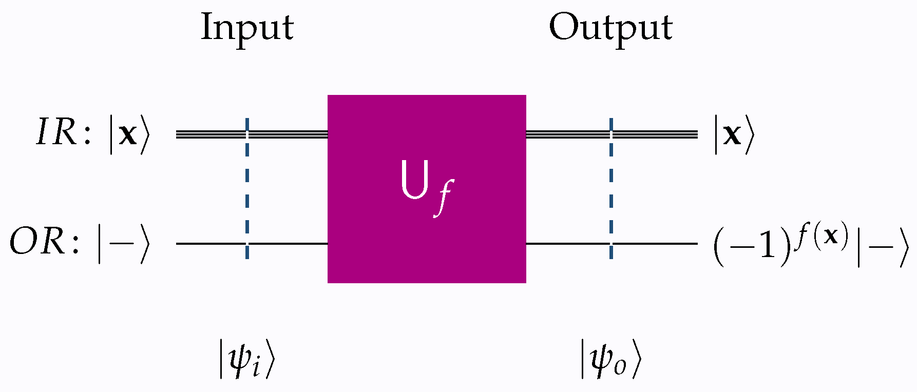
. Let and stand for the perfect superposition state corresponding to two quantum registers, one with 2 and one with 3 qubits, respectively. In such a scenario, the general formula (1) becomes Oracles represent a fundamental concept in quantum computing, serving as components in numerous quantum algorithms. An oracle functions as a black box that encapsulates a particular function or information within a quantum circuit, enabling quantum algorithms to address problems more effectively than classical algorithms in specific scenarios. It facilitates the evaluation of the function or the verification of a condition without disclosing the internal mechanisms of the function. In the realm of quantum algorithms, oracles are frequently employed to identify solutions to a problem or to convey insights regarding a function’s behavior. For the purposes of this discussion, the following definition is adequate.
Definition 2 (Oracle & Unitary Transform)
. An oracle
is a black box implementing a Boolean function f. The idea here is that, being a black box function, we know nothing about its inner working; just that it works correctly. Thus, it can be used for the construction of a unitary transform that captures the behavior of f. Henceforth, we shall assume that the corresponding unitary transform implements the standard schema This particular oracle is occasionally designated as a Deutsch–Jozsa oracle. It is pertinent to mention that there exist other types of oracles, such as the Grover oracle, primarily employed to identify solutions to a problem. The present study assumes that every oracle and unitary transform adheres to Equation (
4) and is utilized to infer a function based on its behavior. The primary measure of complexity in oracular algorithms is the query complexity, defined as the number of queries directed towards the oracle by the algorithm. To obtain any useful information from the schema (
4), we set
equal to
, in which case (
4) takes the following familiar form:
Figure 1 and
Figure 2 give a visual outline of the unitary transforms
that implement schemata (
4) and (
5), respectively.
Throughout this work, the following conventions are consistently applied to all quantum circuits, including those shown in
Figure 1 and
Figure 2.
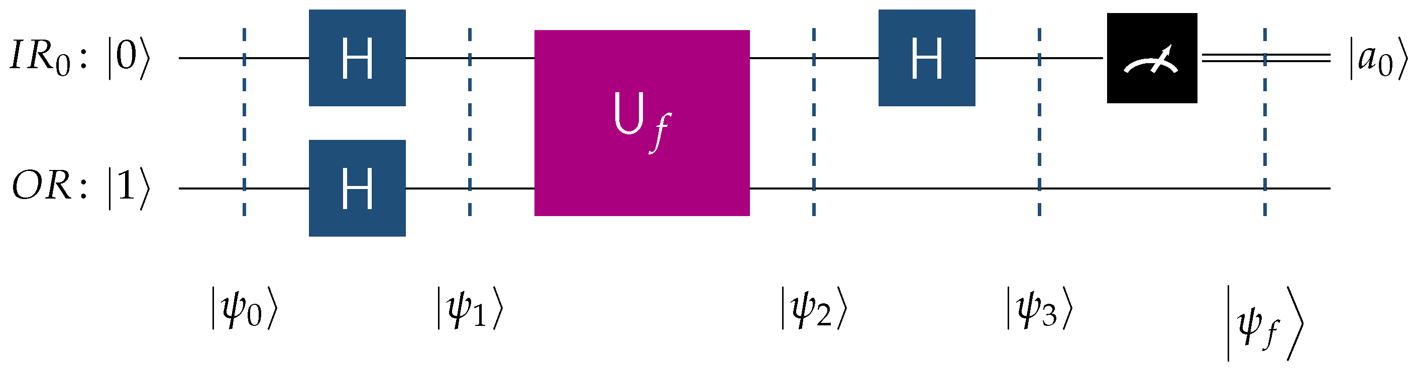
Example 3 (Oracle in Deutsch’s Algorithm)
. Perhaps the earliest quantum algorithm, Deutsch’s algorithm, provides a simple but instructive example of a quantum oracle. This algorithm is mainly a proof of concept, in that it solves a specific problem faster than any classical algorithm. Given a Boolean function , which is either constant (same output for both inputs) or balanced (different outputs for each input), the algorithm determines whether f is constant or balanced using only one query to the function, compared to two queries required classically. The quantum circuit in Figure 3 visualizes the implementation of Deutsch’s algorithm and employs the following notation. is the quantum input register that contains one qubits and starts its operation at state .
is the single-qubit output register initialized to state .
H is the Hadamard transform.
is the unitary transform corresponding to the oracle for the unknown function f. The latter is promised to be constant or balanced.
Referring to Figure 3 and recalling that the ordering the qubits adheres to the Qiskit [44] convention, we may express the initial state as shown below Applying Hadamard gates to all qubits leads to the next state , which, by taking into account (2) and (3), can be written as The oracle’s action according to the schema (5), evolves the state to The power of the quantum oracle stems from its ability to encode both output values of the Boolean function f into the relative phase of state . In the literature, this is referred to as the phase kickback
phenomenon. Phase kickback is a fundamental trait of many quantum algorithms because an operation on the ancilla qubit induces a phase shift on the control qubit. To successfully employ this technique, it is necessary for the ancilla qubit to be in state = = (recall Equation (3)). Using phase kickback is crucial because the oracle instead of writing the values explicitly to a qubit, encodes them as the relative phase . The typical method to produce is to initialize the ancilla qubit to state and, subsequently, apply the Hadamard transform H, as depicted in the quantum circuit of Figure 3. Modern-day quantum computers allow for the immediate initialization of qubits to states other than and , such as . In all of the quantum circuits shown in the rest of this paper, we directly initialize the output register to . Subsequently, by applying the Hadamard gate to the quantum input register , we drive the system into the described below It is easy to see that the amplitude of the state is given by the following formulawhich enables us to distinguish between the following two cases. - (D1)
If f is constant, then (7) reduces to . - (D2)
If f is balanced, then (7) reduces to .
Thus, if we measure , then f is constant, otherwise f is balanced. An important observation is that the quantum oracle demonstrates parallelism by evaluating f on both inputs simultaneously, and interference by amplifying desired outcomes.
We point out that the term “promise” is frequently used in the literature to describe a specific property of the Boolean function f. This means that we are assured, or if you would prefer we are certain with probability , that f satisfies the property in question. One well-known example of this is the Deutsch–Jozsa algorithm, which promises that f is either balanced or constant.
Extending the operation of addition modulo 2 to bit vectors is a natural and fruitful generalization.
Definition 3 (Bitwise Addition Modulo 2)
. Given two bit vectors , with and , we define their bitwise sum modulo
2, denoted by , as Following the standard approach, we use the same symbol ⊕ to denote the operation of addition modulo 2 two between bits, and the bitwise sum modulo 2 between two bit vectors because the context always makes clear the intended operation.
3. The Promised Class
Typically, by employing a quantum classification algorithm, we are able to classify with probability functions that satisfy certain special properties. Most often in the literature, one encounters some phrase that states that we have been given the promise that the classifiable functions fulfill these special properties, hence the “promise” problem. In this work, we refer to the “promised” class to encompass all these functions that satisfy these properties. In our investigation, the promised class is rigorously defined in Definition 13. To dispel any possible ambiguity, we clarify that the classification algorithm is not expected to work correctly, or to be more accurate, is improbable to give the right answer, whenever the input function fails outside the promised class. Implementation-wise, these quantum algorithms make use of an oracle that stealthily implements the input function. The main premise of this work is to investigate if it is possible to gain any information when the input function falls outside the promised class, as rigorously defined in Definition 13. To bear any useful result, such an undertaking must be concrete. Therefore, we shall work under the following hypotheses.
- (H1)
We study the behavior of the quantum classification algorithm BFPQC, introduced in [
43]. The acronym stands for Boolean Function Pattern Quantum Classifier.
- (H2)
BFPQC is designed to classify all Boolean functions belonging to the promised class with probability using just a single oracular query.
- (H3)
In this paper, we study functions that, despite being outside the promised class, are still quite “close” to its elements, in the sense we shall make precise in Definition 19.
Under the above hypotheses, the question we shall answer here is: can we obtain any useful information? And, if so, under what circumstances?
As previously mentioned, we conceptualize this method as the advancement of a game played between our talented stars, Alice and Bob. This game is called the Classification Game and is governed by the following rules.
- (G1)
Bob is free to choose any Boolean function, belonging either to the promised class or to a class near to the promised class as ordained by Definition 19. Bob must announce to Alice the class to which the unknown function belongs.
- (G2)
Bob wins the game if Alice fails to identify the chosen function if it belongs to the promised class, or if Alice fails to obtain any useful information if it is outside the promised class. Otherwise, Alice is the winner.
- (G3)
In terms of implementing the game as a quantum circuit, Bob chooses the hidden oracle, while Alice furnishes the classifier, and is allowed to make a single query to the oracle.
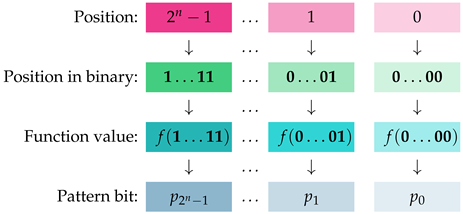
Definition 4 (Pattern Bit Vectors)
. Let f be a Boolean function from to , . We abstract the operation of f into a unique bit vector that we call pattern bit vector. The technicalities are given below.
The pattern bit vector = … corresponding to f is the element of with the property that , where is the binary bit vector representing integer i, . The pattern bit vector codifies the binary values of as ranges over .
The negation of the pattern bit vector = …, denoted by , is the pattern bit vector …, which encodes the function .
Example 4 (Pattern Bit Vectors)
. In the previous Example 1, we defined the Boolean functions f and g, whose values are contained in Table 1. The pattern bit vectors and their negations corresponding to the functions f and g are listed below: Definition 5 (Functions from Patterns Bit Vectors)
. Conversely, to any bit vector = … of length , we associate the Boolean function with the property that , where is the binary bit vector representing integer i, .
In the rest of this paper, to avoid excessive notation, when we want to refer to an arbitrary pattern bit vector without emphasizing the corresponding function f, we shall simply write instead of .
Example 5 (Functions from Patterns Bit Vectors)
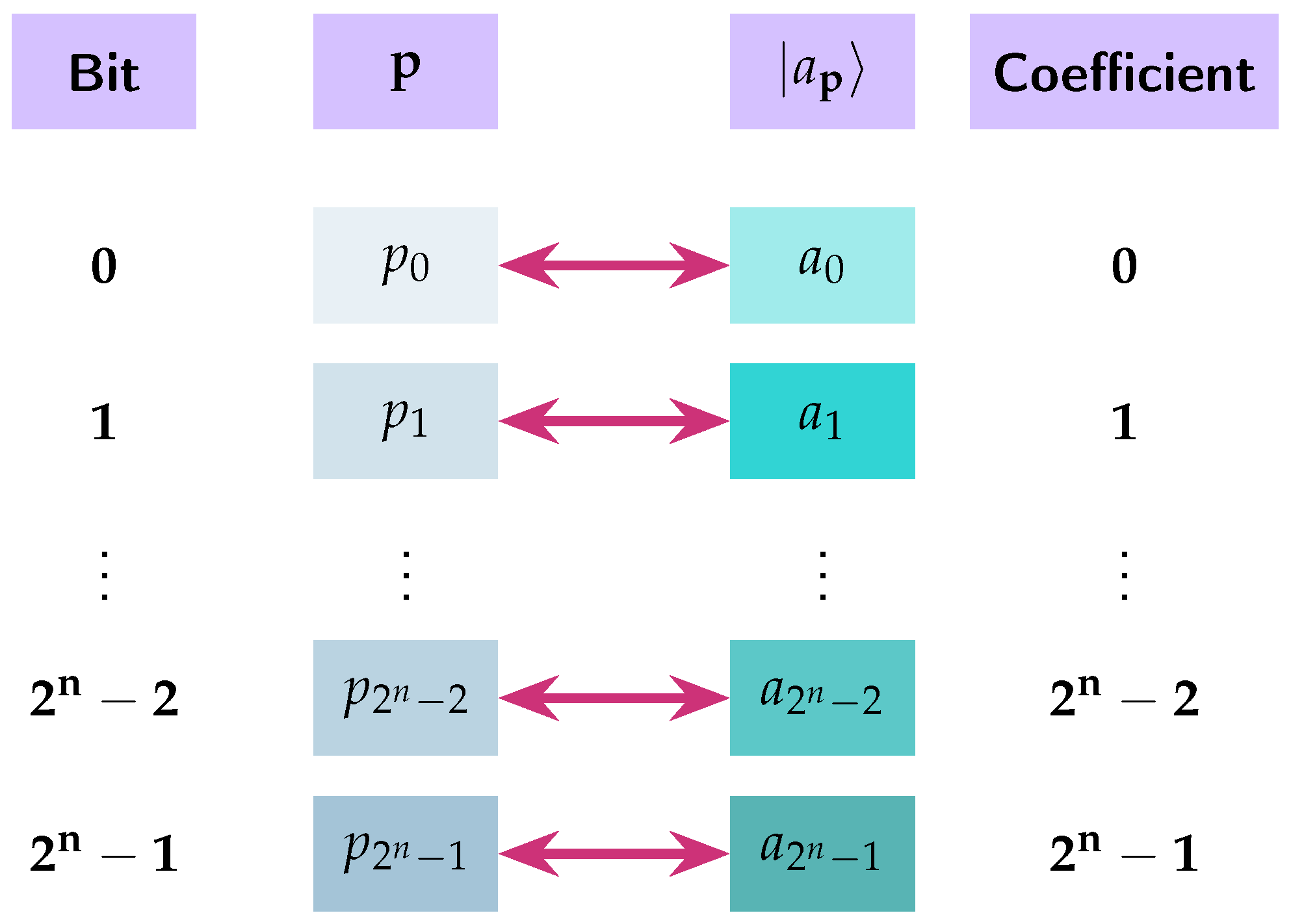
. Let us consider the pattern bit vectors and and let f and g be the Boolean functions that correspond to these bit vectors. The behavior of these functions, i.e., their values as their inputs range over , is given in Table 2. The closed form of functions f and g is described below: Definition 6 (Pattern Kets)
. To each pattern bit vector = …, we associate the -dimensional pattern ket
, with coefficients , , given by the next formula. The visual interpretation of Definition 6 is presented in
Figure 4.
The intuition behind the above Definition 6 is quite straightforward. If
is an oracle realizing the Boolean function
f, then, by recalling (
1), we surmise that
results from the action of
onto the perfect superposition state
. For future reference, we make a rigorous note of this fact in the following relation:
Example 6 (Pattern Kets)
. Recalling the pattern bit vectors and computed in the previous Example 4, and applying Definition 6, we see that the pattern kets and are: If and are oracles for f and g, respectively, their action on the perfect superposition states and , as described in Example 2, will produce the pattern kets and shown above.
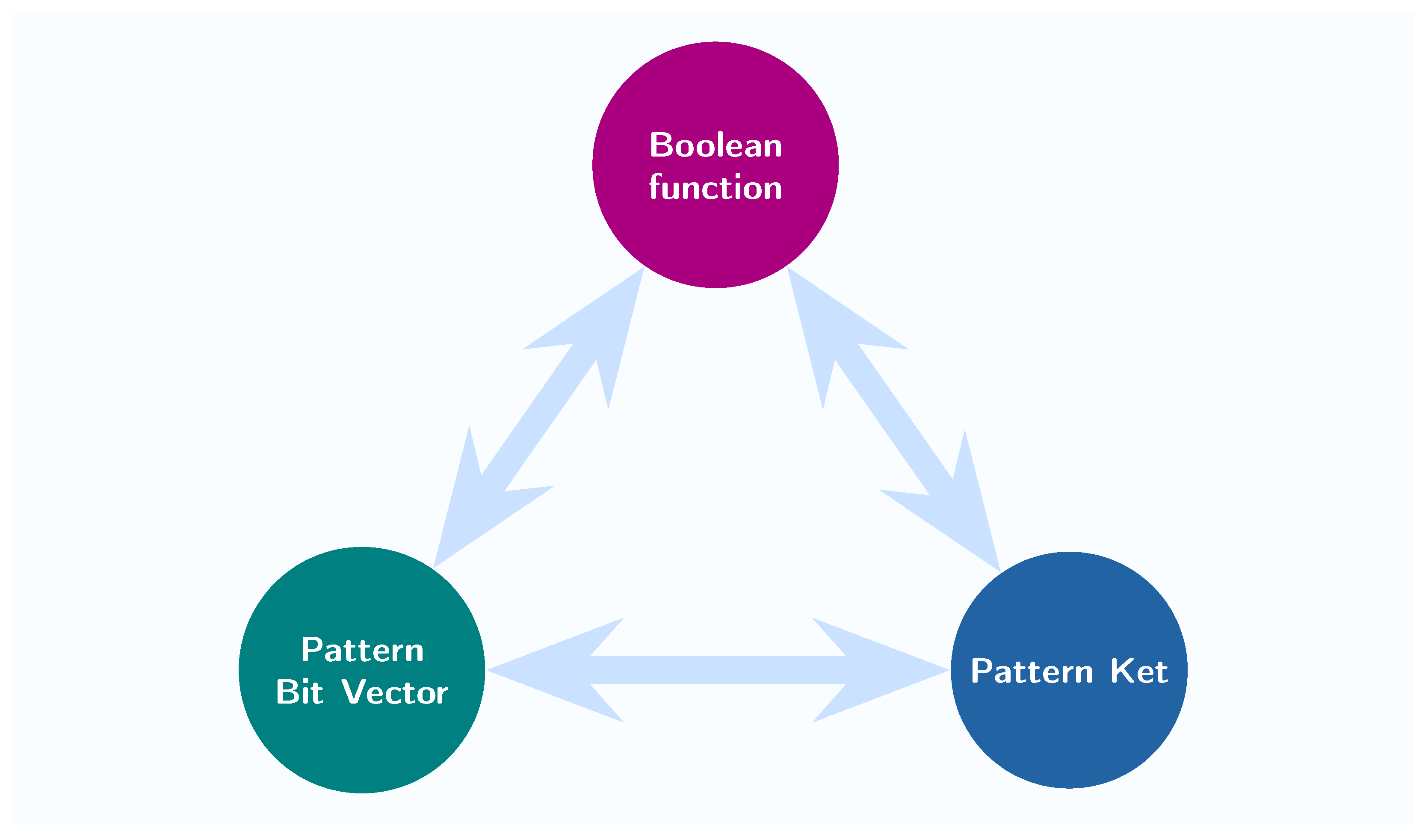
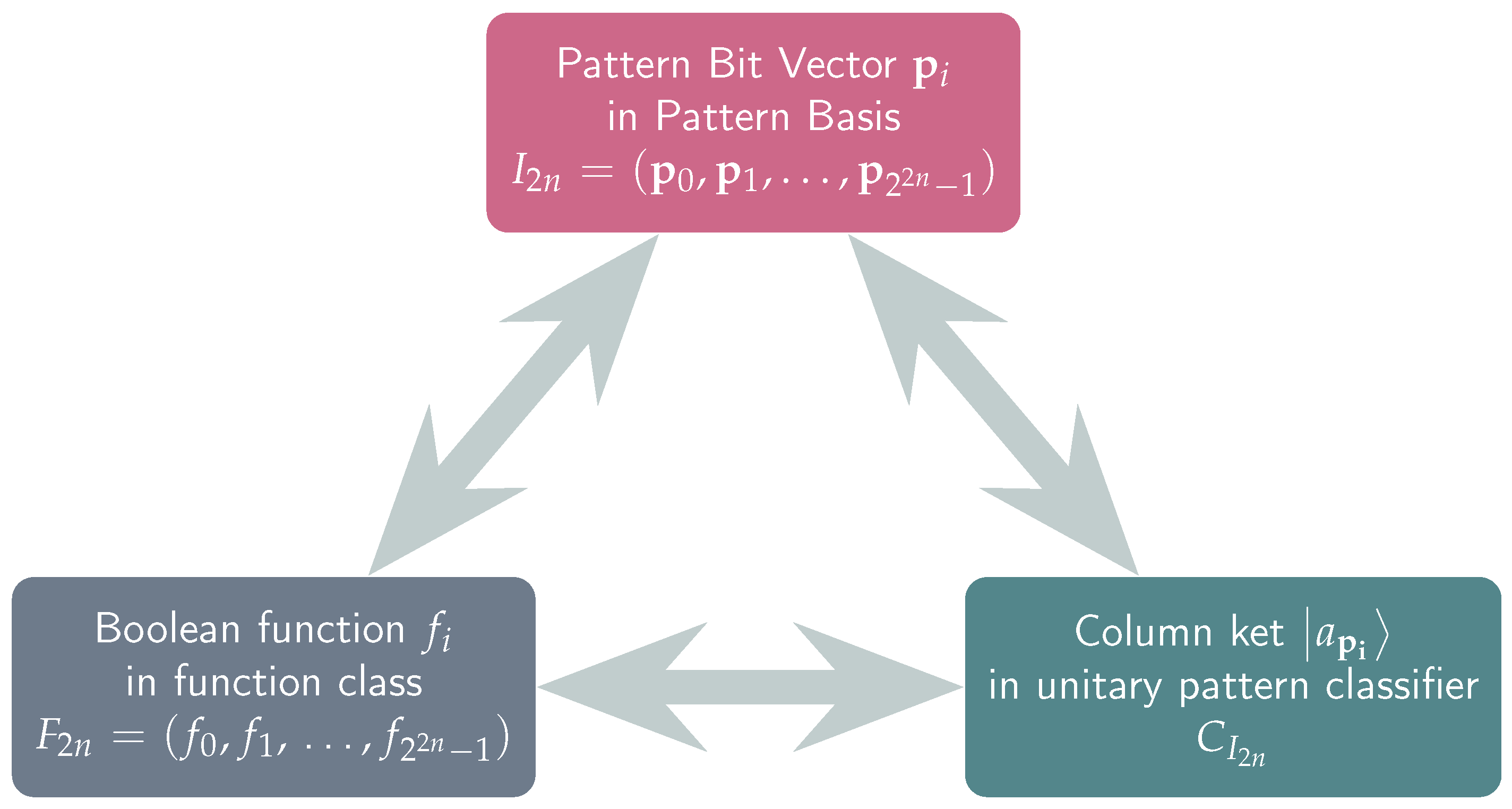
The previous Definitions 4 and 6 clearly illustrate a one-to-one relationship between Boolean functions and pattern bit vectors and between pattern bit vectors and pattern kets. One should consider a Boolean function, its corresponding pattern bit vector, and the corresponding pattern ket as different facets of the same entity. Consequently, understanding the behavior of a Boolean function allows for the creation of its pattern bit vector, or its pattern ket, while any one of the pattern bit vectors or the pattern kets holds all the essential information required to recreate the Boolean function. The next
Figure 5 is meant to convey this strong correlation among these three entities.
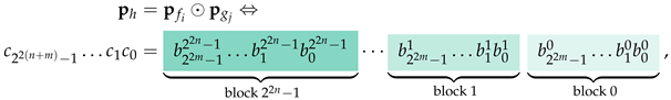
Definition 7 (Pattern Bit Vectors Product)
. Let = … and be two pattern bit vectors of length and , respectively, where, in general, . We define their product, denoted by , as Example 7 (Pattern Bit Vectors Product)
. We explain the product operation between two pattern bit vectors begin by giving two detailed examples: and .To explain all the details, we show the step-by-step product construction process in Table 3 and Table 4. Definition 8 (Orthogonal Pattern Bit Vectors)
. Given two pattern bit vectors and of length , we say that and are orthogonal if contains 0s and 1s.
Definition 9 (Pattern Basis)
. A pattern basis of rank n, , is a list of pairwise orthogonal pattern bit vectors , each of length .
Example 8 (Pattern Bases)
. Consider the following two lists and of pattern vectors: Every has length and is orthogonal to every other , , and, similarly, every has length and is orthogonal to every other , . Furthermore, both lists and consist of pattern bit. Hence, according to Definition 9, and are two different pattern bases of rank 2.
Definition 10 (Pattern Bases Product)
. Let = … and = …, be two pattern bases of rank n and m, respectively, where, in general, . Their product ⊙ is defined ascomprising a list of pattern bit vectors, each of length . We employ the same symbol ⊙ to denote the product operation between two pattern bit vectors, and the product operation between two pattern bases because the context always makes clear the intended operation.
Example 9 (Pattern Bases Product)
. In this example, we construct the product between two pattern bases. We focus on the pattern basis , which is the set consisting of the following four pairwise orthogonal pattern vectors: The intuition behind our choice of the pattern basis is that these pattern vectors correspond to imbalanced binary Boolean functions and can be used to generate a sequence of classes of imbalanced Boolean functions. We compute the product of with itself To show how Definition 10 works, we list the elements of in Table 5, indicating their derivation from . In view of the previous example, it becomes clear that we can define a sequence of classes of imbalanced Boolean functions. To do so, we start from the pattern basis
, already encountered in Example 12, that consists of the following four pairwise orthogonal pattern bit vectors:
Definition 11 (A Sequence of Imbalanced Pattern Bases)
. We recursively define a sequence , of pattern bases exhibiting imbalance.
- (I0)
If , the corresponding pattern basis is , as defined by (13). - (I1)
Given the pattern basis of rank , we define the pattern basis of rank as follows: - (I2)
This sequence of pattern bases , , …, , …, is denoted by .
As we have pointed out, the sequence of pattern bases induces a corresponding sequence of classes of Boolean functions. This concept is formalized by Definition 12.
Definition 12 (Functions from Imbalanced Bases)
. Let = … be a pattern basis of rank . To we associate the class = … of Boolean functions from to such that is the pattern bit vector corresponding to , . This sequence of classes of Boolean functions , , …, , …, is denoted by .
Definition 13 (The Promised Class)
. The promised class is the collection of Boolean functions belonging to the sequence.
In a symmetrical manner, the sequence of pattern bases induces a corresponding sequence of unitary pattern classifiers. This concept is formalized by Definitions 14 and 15.
Definition 14 (Unitary Pattern Classifiers)
. Let = be a pattern basis of rank n, . To corresponds the unitary pattern classifier
, defined as follows: Definition 14 concerns the most general case, where the starting point of the construction is an arbitrary pattern basis. The following Definition 15 is tailored to the special case of imbalanced pattern bases.
Definition 15 (Unitary Pattern Classifiers for Imbalanced Functions). We recursively define a sequence of unitary pattern classifiers corresponding to the sequence of imbalanced pattern bases as follows.
- (CI0)
For , the unitary pattern classifier corresponding to is denoted by , and, in accordance to Definition 14, is given by - (CI1)
Given the unitary pattern classifier corresponding to the pattern basis , we define , corresponding to as - (CI2)
We use for the sequence of unitary pattern classifiers , , …, , … .
Example 10 (Unitary Pattern Classifiers)
. We start by explicitly writing the unitary classifier that corresponds to the pattern basis . Its precise construction follows the guidelines outlined in Definitions 6 and 14. The end result is shown below: Incidentally, we note that can be easily constructed by modern quantum computers using ubiquitous standard gates such as the Hadamard, Z and controlled-Z gates: In the same way, we construct the matrix representation of the unitary classifier , given below. The previous Definitions 11, 12, and 15 clearly illustrate a one-to-one correspondence among the elements of the pattern basis
, the functions of the function class
, and the column kets of the unitary pattern classifier
since they all contain precisely the same information. This situation is captured by the following
Figure 6.
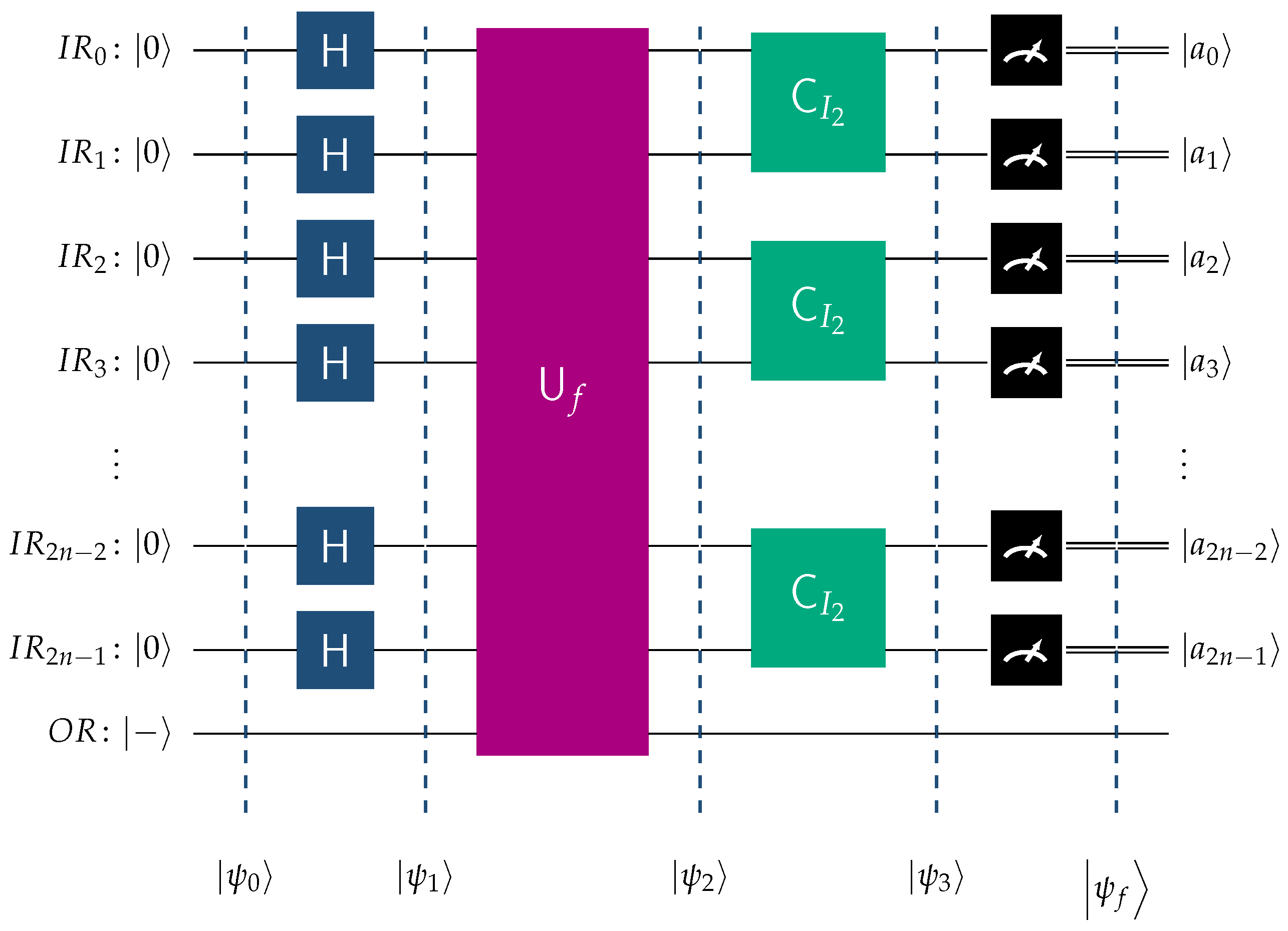
The quantum algorithm BFPQC (Boolean Function Pattern Quantum Classifier), as introduced in [
43], classifies imbalanced Boolean functions that belong to the promised class defined in Definition 13. The primary characteristic of these functions is that the proportion of elements in their domain assigned the value 0 is different from the proportion assigned the value 1. The BFPQC algorithm classifies these functions with a probability of
using a single oracular query. To achieve this, it employs the unitary classifiers
,
, as the main component in the construction of a family of quantum circuits QCPC
2n, for the classification of the class of Boolean functions
. Suppose we intend to classify a Boolean function belonging to the
sequence, and, in particular, to the class
, for some specific
n. This is easily achievable by the quantum circuit QCPC
2n that utilizes as the primary component the unitary classifier
. This quantum circuit is depicted in
Figure 7. If the oracle encodes a function of
, the QCPC
2n circuit will conclusively, i.e., with probability
, determine this function.
To enhance clarity, we explain the notation used in the above figure.
is the quantum input register that contains qubits and starts its operation at state .
is the single-qubit output register initialized to .
H is the Hadamard transform.
is the unitary transform corresponding to the oracle for the unknown function h.
is the fundamental building block of
, as evidenced by Equation (
17).
The situation is summarized in the following Theorem 1 proved in [
43]. To enhance the readability of this article, we have relocated the proofs of all results in
Appendix A.
Theorem 1 (Classification in the Promised Class). Let , , be a Boolean function contained in the class = …. Upon measuring the quantum circuit QCPC2n containing the oracle for and the unitary classifier , we obtain , where is the binary representation of the index i, and is one of the basis kets of the computational basis.
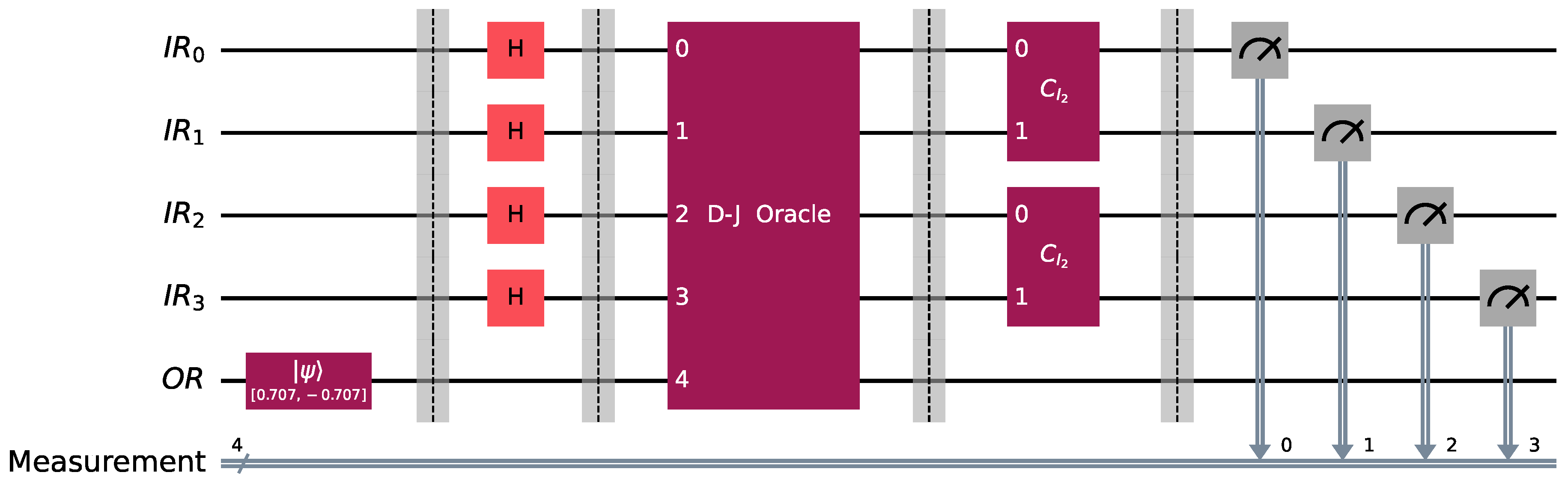
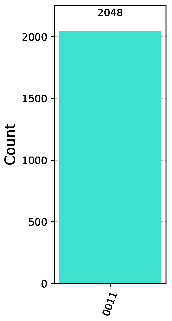
Example 11 (Classifying functions in the Promised Class)
. Suppose that, in the Classification Game between Bob and Alice, Bob chooses a Boolean function from , which belongs to the promised class of functions. Say that Bob chooses , the behavior of which is encoded by the pattern vector , listed in Example 12. Alice makes her move by employing the classifier . In this case, the concrete implementation in Qiskit [44] of the classification algorithm takes the form shown in Figure 8, where Bob uses the oracle for the function and Alice the classifier . After the action of the classifier, the state of the system is just . Therefore, measuring the quantum circuit depicted in Figure 8 will output the bit vector 0011 with probability 1 (as corroborated by the measurements contained in Figure 9), which is the binary representation of the index of . Alice surely wins the game, as anticipated. This article aims to explore the information that can be derived from the BFPQC algorithm when the input is a function that, while not part of the promised class, remains relatively close, in a way to be rigorously defined in Definition 19. When the oracle realizes a function outside , the final measurement will not reveal the function. However, as we shall demonstrate, it is possible to obtain some useful information when the input function is sufficiently close to the class , in the sense of Definition 19.
4. Outside the Promised Class
For our investigation regarding the behavior of functions outside the promised class, we shall consider functions that are a mixture of balanced and imbalanced Boolean functions. We begin by first defining the sequence of balanced pattern bases, as outlined in the next Definition 16. To avoid any confusion, we clarify that only the first pattern bit vector in every basis represents the constant function; all the remaining pattern bit vectors encode balanced functions.
Definition 16 (A Sequence of Balanced Pattern Bases)
. We recursively define a sequence , of pattern bases demonstrating balanced behavior.
- (B0)
If , the corresponding pattern basis is , as defined below - (B1)
Given the pattern basis of rank , we define the pattern basis of rank as follows: - (B2)
This sequence of pattern bases , , …, , …, is denoted by .
Example 12 (Pattern Bases Product)
. In this example, we construct the pattern basis . Starting from the initial pattern basis , as defined by Equation (21), we construct the product of with itself Using Definition 10, we compute the elements of in Table 6, indicating their derivation from . As we have pointed out before, only the first pattern bit vector in represents the constant function, and all the remaining pattern bit vectors encode balanced functions.
Definition 17 (Functions from Balanced Bases)
. Let = … be a balanced pattern basis of rank . To we associate the class = … of Boolean functions from to such that is the pattern bit vector corresponding to , . This sequence of classes of Boolean functions , , …, , …, is denoted by .
It is clear that the pattern bit vectors in correspond to binary functions outside . These particular pattern bit vectors are inspired from the 2-fold Hadamard transform .
Example 13 (Inability to classify functions outside the Promised Class)
. Although the BFPQC can conclusively classify all the functions that lie within the promised class , it fails, as expected, to classify functions outside the promised class. It is straightforward to see that given any , , the corresponding function cannot be classified by BFPQC. The explanation for this behavior is the following. The pattern kets corresponding to the bit vectors of arewhich are precisely the columns of . Accordingly, the action of the classifier on any of them will result in one of the following stateswhich, upon measurement, will collapse of any of the four basis states with equal probability . This line of reasoning leads to Theorem 2, which is proved in
Appendix A.
Theorem 2. Let , , be a Boolean function contained in the class = …. The state of the input register in the quantum circuit QCPC2m that contains the oracle for and the unitary classifier , before measurement isUpon measurement of the input register , we may obtain any of the basis kets of the computational basis with equal probability , rendering classification probabilistically impossible. Definition 18 (Extended Product)
. Let and be two Boolean functions. We construct their extended product
, denoted by , as the Boolean function defined as follows: Example 14 (Extended Product Example)
. This example explains how the extended product between Boolean functions works. Consider two functions from the class , say and , corresponding to pattern bit vectors and from (12). The detailed construction of their extended product function is contained in Table 7. The pattern bit vectors and the pattern kets of , and are shown in Table 8. The resulting function belongs to the class , and the corresponding pattern bit vector is listed in Table 5, as . As we have previously explained, our aim is to study what information can be obtained by the BFPQC algorithm if the input function is outside the promised class, but, at the same time “close” to some function of the sequence. The next Definition 19 formalizes this concept of nearness.
Definition 19 (Left & Right Clusters)
. Let and , , be two classes of functions in the and sequences, respectively. We define the following two concepts.
The left cluster of by , denoted by , is the class of Boolean functions of the form , where and . We refer to the function as being in the left cluster of f.
The right cluster of by , denoted by , is the class of Boolean functions of the form , where and . In this case, we say that the function is in the right cluster of f.
Henceforth, we shall consider any function in as being close to every function in the left or right cluster of by .
Example 15 (Functions in the Left and Right Cluster)
. Suppose that we are given a function belonging to the sequence, say , that corresponds to the pattern bit vector . Let us also consider a function from the sequence, say , corresponding to the pattern bit vector . The truth values of and are listed in Table 2 of Example 5. Using and , we may construct the new functions and that belong to the left and right cluster of , respectively. The detailed construction of and , according to Definition 18, produces the truth values contained in Table 9. From Table 9, we immediately surmise that and are the pattern bit vectors of the Boolean functions and , respectively. From now on, we assume that the oracle in
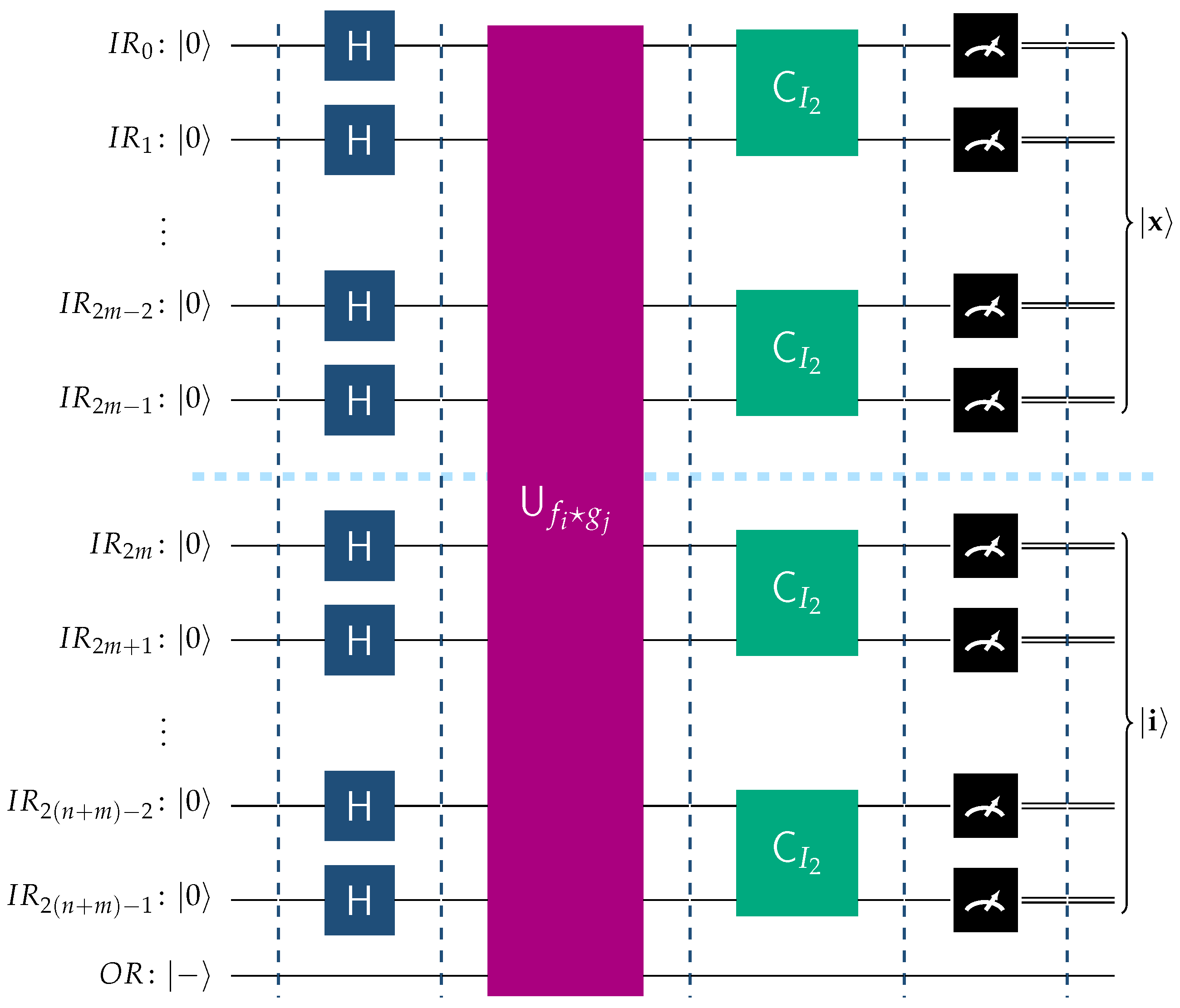
Figure 7 realizes a function
h that is either in the left, or right cluster of
. It is convenient to distinguish the following two cases, depending on whether the function
h belongs to the left or right cluster of
.
Suppose that
, where
and
with corresponding indices
i and
j, respectively. The appropriate circuit in this scenario is depicted in
Figure 10. In this case,
In view of Theorems 1 and 2, we arrive at the following relation
This is the state of the input register of the system prior to the final measurement. Hence, upon measurement, the final outcome in the input register will be , that is the most significant qubits will contain a random basis ket from , and the least significant qubits will contain , which correctly identifies the function belonging to .
Suppose that
, where
and
with corresponding indices
i and
j, respectively. This situation is visualized in
Figure 11. Resorting to the same reasoning as in the previous case, we see that
Invoking Theorems 1 and 2, we derive the following relation
Therefore, upon measurement, the input register will contain . Now the most significant qubits will contain , correctly identifying the function belonging to , and the least significant qubits will contain a random basis ket from .
Figure 10.
This figure shows the operation of the BFPQC circuit for the function .
Figure 10.
This figure shows the operation of the BFPQC circuit for the function .
Figure 11.
The above figure depicts the operation of the BFPQC circuit for the function .
Figure 11.
The above figure depicts the operation of the BFPQC circuit for the function .
Example 16 (Functions Outside the Promised Class)
. In this example we consider two possible rounds of the Classification Game played by Alice and Bob.
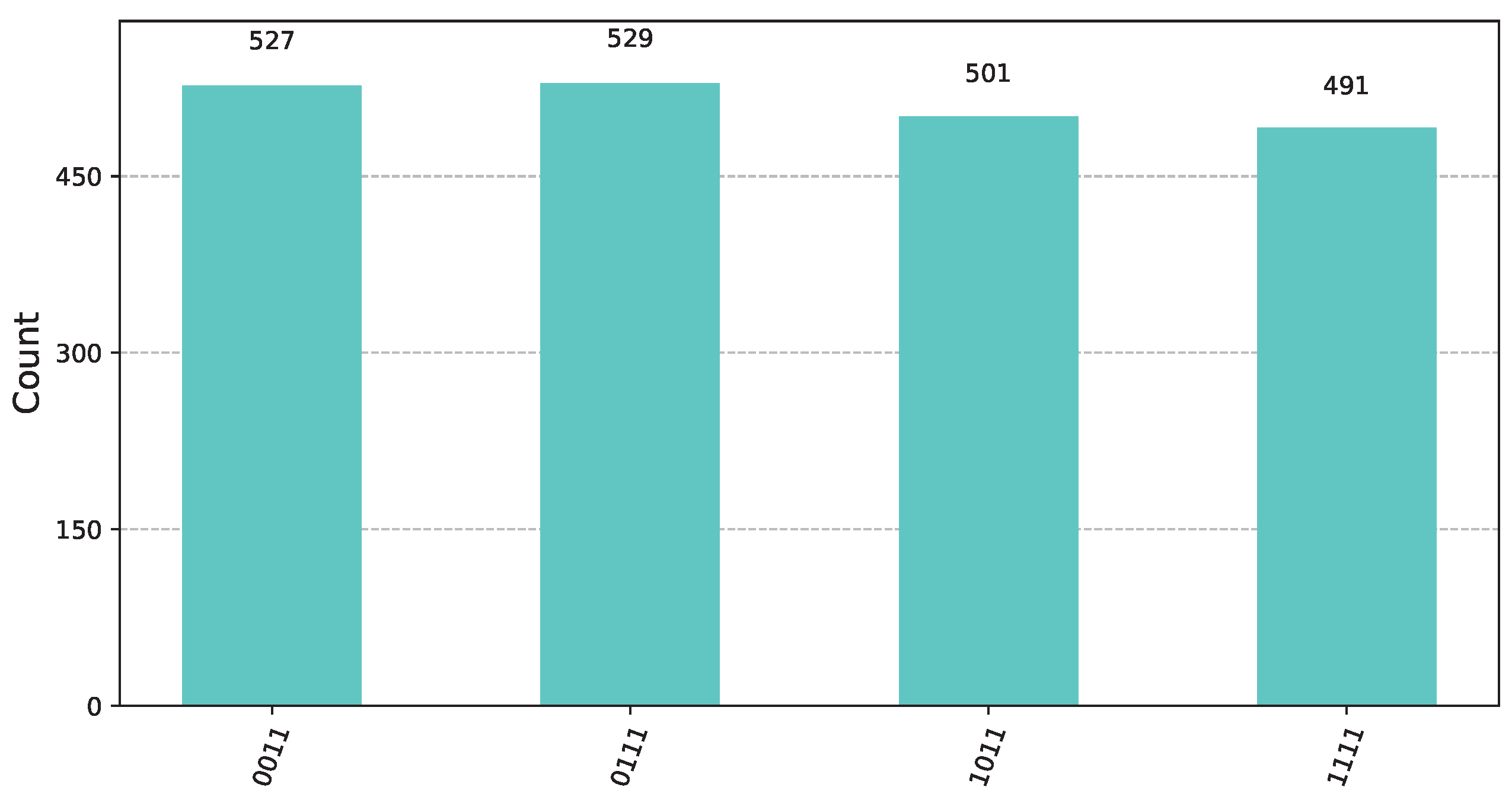
![Computers 14 00228 i001]() Let us suppose that in the first round, Bob chooses a function from the left cluster , say . Function is from the class and corresponds to the pattern bit vector from (21), while is from corresponding to the pattern bit vector from (13). According to the rules of the Classification Game, as explained in Section 3, Bob announces to Alice the underlying class that he has chosen. We note that this is the only information known to Alice. Subsequently, Bob constructs the oracle for the secret function . In this scenario, Alice must use the unitary pattern classifier = from Definition 15. For this particular instance, the circuit, with the exception of the oracle furnished by Bob, takes the concrete implementation visualized in Figure 8. By applying (26) we see that the state of the input register prior to the final measurement is
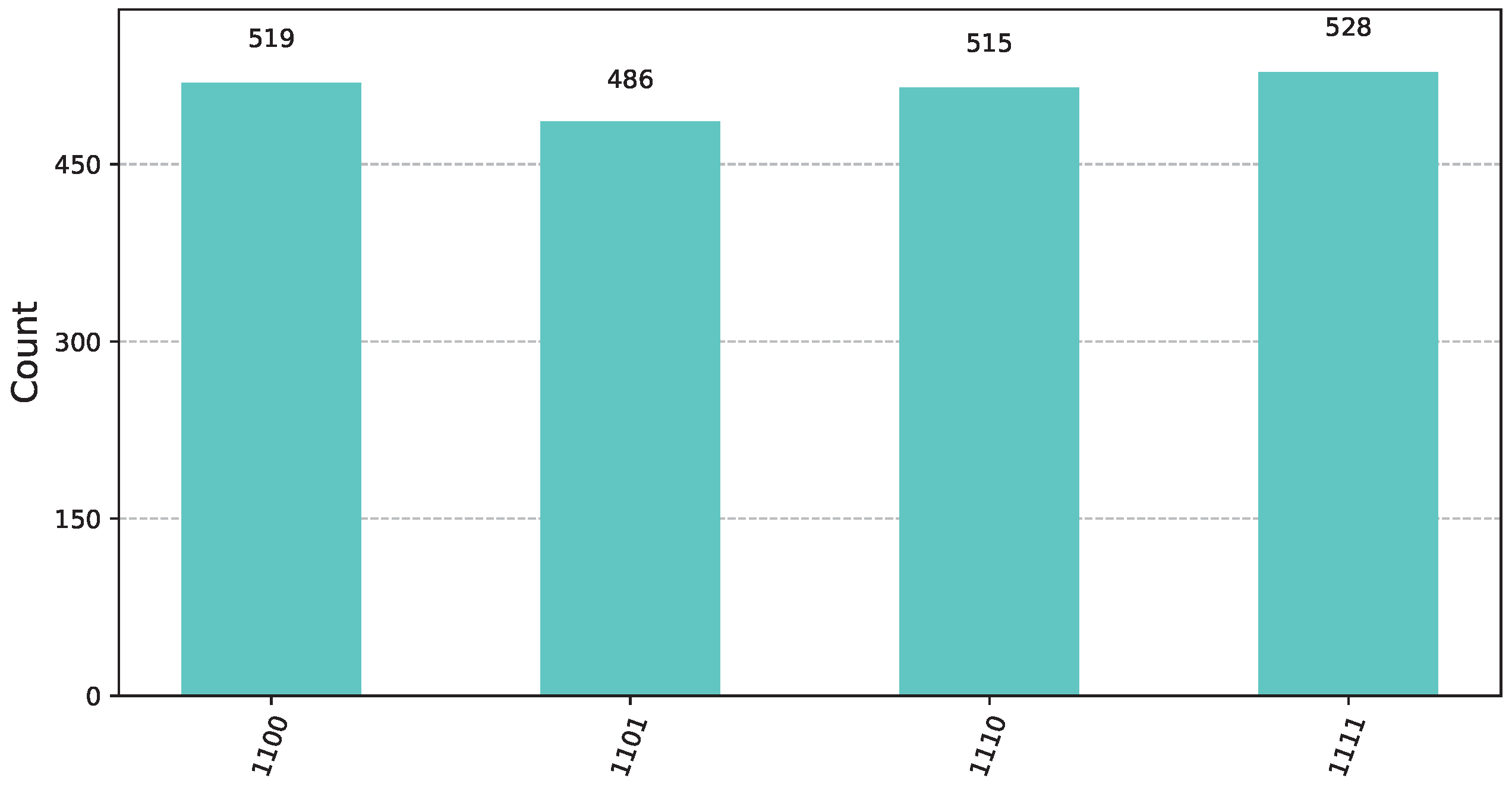
Let us suppose that in the first round, Bob chooses a function from the left cluster , say . Function is from the class and corresponds to the pattern bit vector from (21), while is from corresponding to the pattern bit vector from (13). According to the rules of the Classification Game, as explained in Section 3, Bob announces to Alice the underlying class that he has chosen. We note that this is the only information known to Alice. Subsequently, Bob constructs the oracle for the secret function . In this scenario, Alice must use the unitary pattern classifier = from Definition 15. For this particular instance, the circuit, with the exception of the oracle furnished by Bob, takes the concrete implementation visualized in Figure 8. By applying (26) we see that the state of the input register prior to the final measurement isFigure 12 shows the state of the input register prior to measurement. Upon measurement, the input register will be , for some random . Practically, this means that, while the 2 most significant qubits will contain a random basis ket from , the 2 least significant qubits will contain 11. This will conclusively reveal that the second operand in the unknown extended product is the function. Therefore, Alice will win the first round. ![Computers 14 00228 i002]() For the second round, Bob now picks a function from the right cluster , specifically the function . Functions and , with pattern bit vectors from (13) and from (21), belong to the classes and , respectively. As ordained by the rules of the Classification Game, given in Section 3, Bob informs Alice that he has picked a function from the right cluster . Subsequently, Bob constructs the oracle for the unknown function . Alice, knowing only that the unknown function belongs to the right cluster , employs the unitary pattern classifier = from Definition 15. For this round, the quantum circuit, with the exception of the oracle furnished by Bob, resembles the implementation depicted in Figure 8. By applying (28), Alice concludes that the state of the input register prior to the final measurement is
For the second round, Bob now picks a function from the right cluster , specifically the function . Functions and , with pattern bit vectors from (13) and from (21), belong to the classes and , respectively. As ordained by the rules of the Classification Game, given in Section 3, Bob informs Alice that he has picked a function from the right cluster . Subsequently, Bob constructs the oracle for the unknown function . Alice, knowing only that the unknown function belongs to the right cluster , employs the unitary pattern classifier = from Definition 15. For this round, the quantum circuit, with the exception of the oracle furnished by Bob, resembles the implementation depicted in Figure 8. By applying (28), Alice concludes that the state of the input register prior to the final measurement isFigure 13 shows the state of the input register prior to measurement. Upon measurement, the input register will be , for some random . Hence, the 2 most significant qubits will contain 11, while the 2 least significant qubits will contain a random basis ket from . Thus, Alice will correctly identify the first operand of the of the extended product as being , and win the second round too. 6. Discussion and Conclusions
6.1. Synopsis
Advanced research on the classification of Boolean functions that satisfy specific properties, i.e., belong to a particular class, is abundant in the literature. Yet, to the best of our knowledge, no prior studies have examined what information might be revealed when the input Boolean function does not fall into this category. This paper offers a fresh research perspective that demonstrates that significant knowledge can still be obtained under appropriate circumstances.
In this paper, we studied what information may be gained when a specific classification algorithm is applied to functions that do not belong to the promised class, but are still relatively close to its elements. For this purpose, we have introduced a novel concept that defines “nearness” between Boolean functions. We illustrate this concept by showing that, as long as the input function is close enough to the promised class, the classification algorithm can still yield insightful information about its behavioral pattern. To the best of our knowledge, this study is the first to demonstrate the benefits of using quantum classification algorithms to look at functions that are not part of the promised class in order to get a glimpse of important data.
In concluding this subsection, we wish to highlight the inherent limitations of our quantum classification framework, particularly when dealing with functions outside the promised class, and to provide guidance for future research directions. When the unknown function lies outside the designated class, it becomes essential to introduce a well-defined notion of distance to quantify its proximity to the promised class, thereby enabling meaningful classification outcomes. To corroborate this, we have conducted extensive experimental simulations using randomly generated Boolean functions that fall outside the promised class. These experiments suggest that, in such random scenarios, the BFPQC algorithm struggles to extract useful information without additional constraints. Consequently, we advocate that for any quantum classification algorithm, including ours, to effectively handle functions outside the promised class, some form of proximity condition must be satisfied to ensure the function is sufficiently “close” to the class. In our framework, the concept of left and right cluster proximity serves as a suitable criterion for defining this nearness, providing a structured approach to assess how closely an unknown function aligns with the promised class. However, other alternative distance metrics could also be considered, each with its own merits and challenges. For instance, the Hamming distance, which measures the number of inputs where two functions differ, represents a straightforward and viable option, though its effectiveness may be limited in the quantum setting due to the projective nature of quantum states, which emphasizes phase and amplitude relationships over simple value differences. Our analysis strongly suggests that imposing a distance-based constraint is critical for any quantum classification algorithm to yield useful insights when dealing with functions outside the promised class.
| Synopsis |
| When the unknown input function h belongs to the left or right cluster of a function f
within the promised class, meaning that h can written either as g⋆f, or f⋆g, where
g, and, thus, h is outside the promised class, the classification algorithm BFPQC can
conclusively unveil f with a single query. This furnishes important information
about the behavioral pattern of h, albeit not the complete information. |
6.2. Additional Possibilities
In our view, one of the most critical and intellectually stimulating directions for advancing the concept of classification—both within and beyond the promised class—lies in generalizing these methodologies to functions defined from , where , . This research direction offers substantial promise, particularly due to the natural compatibility of the Quantum Fourier Transform (QFT) with this task, as it provides a powerful tool for analyzing functions in the Fourier domain. Nevertheless, the transition to this broader domain introduces significant technical challenges that warrant careful consideration. These challenges include the effective generalization of quantum oracles to handle modular arithmetic over , the efficient implementation of the QFT for larger state spaces, and the adaptation of the classification framework to accommodate the increased complexity of both the domain and codomain. Regarding the selection of an appropriate distance metric for comparing such functions, several viable options exist, yet no single approach stands out as the definitively optimal. For example, while the Hamming distance can be straightforwardly extended to count the number of positions where two functions differ, the projective nature of quantum systems may limit its effectiveness in capturing the nuances of quantum states. Consequently, alternative metrics, such as the Fourier-based distance, which leverages the QFT to compare functions in the frequency domain, may offer a more suitable approach for quantum classification tasks.
This investigation, for concreteness, employs the Boolean Function Pattern Quantum Classifier (BFPQC) algorithm, designed to classify imbalanced Boolean functions within a well-defined hierarchy of function classes, denoted
,
, …,
, …. This hierarchy is derived from a corresponding sequence of imbalanced pattern bases,
,
, …,
, …, as rigorously established in Definition 5. Each pattern basis
serves as the structural foundation for constructing the function class
, enabling the BFPQC algorithm to systematically categorize Boolean functions based on their syntactical characteristics. Drawing on the principles outlined in [
43], this framework allows for the development of tailored variants of the BFPQC algorithm, designed to classify diverse classes of Boolean functions by modifying the pattern bases or classification methodologies. For instance, the pattern basis
encapsulates Boolean functions that are either constant or perfectly balanced, providing a foundational example within the hierarchy. To extend this classification to other hierarchical levels, one can revise Definition 14 to redefine the classification process. A particularly effective approach involves defining a new hierarchy of unitary classifiers, as specified in Equation (
37). This results in an alternative hierarchy of Boolean function classes, each incorporating both perfectly balanced and imbalanced functions, thereby expanding the algorithm’s applicability. These modifications not only enhance the versatility of the BFPQC algorithm but also pave the way for further exploration of Boolean function classification in computational and quantum domains, offering potential applications in areas such as quantum algorithm design and pattern recognition.
6.3. Future Research
One research direction that we believe is worth pursuing in the near future is to investigate the viability of encoding strategies in some famous games, such as the Repeated Prisoners’ Dilemma, as Boolean functions. In the Repeated Prisoners’ Dilemma, each player chooses a strategy that dictates their action (Cooperate or Defect) in each round. For a finite number of rounds, strategies like “Tit-for-Tat”, “Grim Trigger”, or “Always Defect”, can be modeled as Boolean functions by associating C to 0 and D to 1, or vice versa. In the quantum setting, a strategy can be implemented as a secret oracle that computes the player’s action. Therefore, given two players with strategies f and g, we believe it will be interesting to examine whether their oracles can be queried to simulate the game’s progression, allowing the analysis of their interaction via the extended product . The classification of as the evaluation of payoffs could be viable because the joint actions at each round determine the payoff matrix entries. Hopefully, by analyzing , one may compute expected payoffs over multiple rounds or characterize the strategy pair’s behavior by determining cooperative or defective tendencies.


 ,
, 

 Let us suppose that in the first round, Bob chooses a function from the left cluster , say . Function is from the class and corresponds to the pattern bit vector from (21), while is from corresponding to the pattern bit vector from (13). According to the rules of the Classification Game, as explained in Section 3, Bob announces to Alice the underlying class that he has chosen. We note that this is the only information known to Alice. Subsequently, Bob constructs the oracle for the secret function . In this scenario, Alice must use the unitary pattern classifier = from Definition 15. For this particular instance, the circuit, with the exception of the oracle furnished by Bob, takes the concrete implementation visualized in Figure 8. By applying (26) we see that the state of the input register prior to the final measurement is
 For the second round, Bob now picks a function from the right cluster , specifically the function . Functions and , with pattern bit vectors from (13) and from (21), belong to the classes and , respectively. As ordained by the rules of the Classification Game, given in Section 3, Bob informs Alice that he has picked a function from the right cluster . Subsequently, Bob constructs the oracle for the unknown function . Alice, knowing only that the unknown function belongs to the right cluster , employs the unitary pattern classifier = from Definition 15. For this round, the quantum circuit, with the exception of the oracle furnished by Bob, resembles the implementation depicted in Figure 8. By applying (28), Alice concludes that the state of the input register prior to the final measurement is
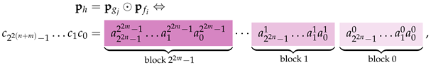
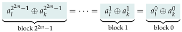
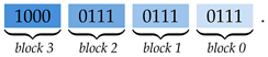
 or
or  . She only requires a single additional bit in any block to know the entire block. Furthermore, Alice concludes that the modulo 2 sum of any two distinct bits of the same block is equal to the modulo 2 sum of the corresponding bits in every other block, e.g., the least two significant bits in every block sum up to 0.
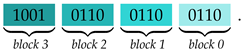
