Enhancing Injector Performance Through CFD Optimization: Focus on Cavitation Reduction

Abstract

The use of computer-aided engineering (CAE) tools has become essential in modern design processes, significantly streamlining mechanical design tasks. The integration of optimization algorithms further enhances these processes by facilitating studies on mechanical behavior and accelerating iterative operations. A key focus lies in understanding and mitigating the detrimental effects of cavitation on injector surfaces, as it can reduce the injector lifespan and induce material degradation. By combining advanced numerical finite element tools with algorithmic optimization, these adverse effects can be effectively mitigated. The incorporation of computational tools enables efficient numerical analyses and rapid, automated modifications of injector designs, significantly enhancing the ability to explore and refine geometries. The primary goal remains the minimization of cavitation phenomena and the improvement in injector performance, while the collaborative use of specialized software environments ensures a more robust and streamlined design process. Specifically, using the simulated annealing algorithm (SA) helps identify the optimal configuration that minimizes cavitation-induced effects. The proposed approach provides a robust set of tools for engineers and researchers to enhance injector performance and effectively address cavitation-related challenges. The results derived from this integrated framework illustrate the effectiveness of the optimization methodology in facilitating the development of more efficient and reliable injector systems.

1. Introduction

Cavitation is a complex and partially understood phenomenon influenced by multiple factors such as vibration and erosion. In an early study, the authors in [1] analyzed cavitation in the cylinder liner of an engine, observing that vibration between components during combustion promoted its occurrence. More recently, the researchers in [2] employed Reynolds-averaged Navier–Stokes (RANS) equations to analyze fluid turbulence, emphasizing the need for further studies to quantify the damage and risks associated with cavitation in diesel fuel injectors. Computational fluid dynamics (CFD) has been instrumental in advancing the understanding and management of cavitation. The studies in [3,4] employed CFD to optimize the design of cavitating jet nozzles and diesel injection nozzles, respectively, highlighting the critical role of pressure and geometry in cavity formation. Building upon these approaches, the present work introduces a novel optimization methodology based on the simulated annealing algorithm, integrated with CFD analysis, to enhance the prediction and control of cavitation behavior. The model was validated through numerical comparison with the results reported in [3], under similar operating conditions, demonstrating strong agreement in cavitation distribution and pressure drop. Similarly, the investigations in [5,6] highlighted the importance of these factors in optimizing engine performance and preventing erosion. Additional research, such as the work in [7,8], provided crucial insights for the design and durability of diesel injection systems, utilizing CFD to predict cavitation erosion and enhance injector reliability. The findings in [9,10,11] further emphasized the impact of geometry and other configurations on flow and efficiency, reinforcing the relevance of CFD in industrial applications.

Geometric optimization is crucial in modern engineering to develop efficient and effective solutions. The studies in [12,13] discussed optimal design and the simulated annealing (SA) algorithm, a stochastic method that is effective for combinatorial and continuous optimization problems. Although SA encounters challenges in the early high-temperature stages where it accepts suboptimal solutions, the improvements proposed in [14] enhanced its convergence by introducing a temperature-dependent penalty function. Additionally, the review presented in [15] proposed variations and strategies such as adaptive cooling and promising neighborhood generation to enhance SA efficiency. The approach in [16] introduced cultural algorithms, combining population-based search techniques with cultural learning mechanisms to address complex optimization problems.

To enhance the efficiency of the optimization process, it is crucial to implement computational strategies that allow for seamless integration between numerical analysis and algorithmic evaluation. In this context, the use of Ansys^® Fluent in journal mode has emerged as a valuable approach, enabling the automation of CFD simulations through scripting. The journal mode allows for the execution of predefined sequences, such as geometry import, meshing, solver setup, and post-processing, without manual intervention, significantly reducing the processing time and ensuring consistency across multiple iterations. When combined with external platforms like MATLAB R2022a, this workflow becomes even more powerful. MATLAB can dynamically modify input parameters, control the journal execution, and retrieve results to evaluate them using the simulated annealing (SA) algorithm. This computational synergy provides a robust framework for design optimization, where the model is continuously updated based on the algorithm’s feedback. Such integration facilitates the identification of an optimal configuration that minimizes cavitation (volume fraction) while maintaining stable pressure and velocity profiles, as highlighted in the development of a model where the input variables serve as primary data for optimization. This integrative approach ensures rapid adaptability and precision in the design process.

2. Theory

2.1. Cavitation

Cavitation occurs when vapor bubbles form in a liquid due to a local pressure drop below the liquid’s vapor pressure. This phenomenon is particularly critical in fluid systems as it can induce vibrations, noise, and unexpected material degradation if not properly predicted and managed. The formation and subsequent collapse of these vapor bubbles generate high-pressure shock waves, which can lead to surface erosion and significantly reduce the lifespan of hydraulic components [8]. During cavitation, mass transfer occurs between the liquid and vapor phases, governed by evaporation and condensation processes, which are highly dependent on thermodynamic and fluid dynamic conditions [8]. The local pressure fluctuations play a crucial role in determining the size, growth rate, and collapse intensity of cavitation bubbles. The studies in [7,9] demonstrated that these rapid pressure variations influence the inception of cavitation and its destructive potential, particularly in high-speed fluid flows.

Moreover, the interaction between vapor bubbles and turbulent flow structures was analyzed in [5,6], highlighting how turbulence intensity can accelerate cavitation onset and amplify its effects. The presence of high shear stresses in the flow can further promote asymmetric bubble collapse, leading to localized surface fatigue and structural weakening. Understanding and accurately predicting cavitation is essential for optimizing the design of fluid systems and establishing appropriate operating parameters. The research in [3,4] showed that computational fluid dynamics (CFD) simulations are valuable tools for modeling cavitation behavior and evaluating different design modifications to mitigate its impact. By integrating cavitation models with advanced optimization algorithms, as proposed in [12,13], it is possible to develop more efficient and durable components that minimize cavitation-induced damage while maintaining optimal fluid performance.

2.2. CFD

Computational fluid dynamics (CFD) is a branch of fluid mechanics that utilizes numerical algorithms and methods to solve and analyze flow-related problems [17]. In Reference [1], the authors provide an overview of the CFD principles and their applications, highlighting its importance in engineering and scientific research. Among the various CFD tools available, Ansys^® stands out as an advanced software that employs these methods to simulate the behavior of products and industrial processes. As demonstrated in [2], the use of Ansys^® significantly reduces the production time and costs compared with traditional experimentation, making it an essential tool in modern engineering. CFD focuses on how fluid motion affects the interaction between the flow and design structures, providing a highly effective analytical tool. Additionally, as discussed in [3], CFD serves as an educational resource that enables students to apply fundamental concepts to real-world situations, enhancing their understanding of fluid dynamics.

The CFD methodology is fundamentally based on the governing equations of fluid dynamics, which mathematically express the conservation laws of physics [3]:

• The conservation of mass for the fluid

$$\left({\displaystyle \frac{\partial \rho }{\partial t}}\right)+\nabla \cdot \left(\rho v\right)=0$$

(1)

where ρ is the fluid density and v is the velocity vector. This allows determining how the fluid mass is distributed and varies over time, which is essential for accurately representing flow behavior, especially in fluid dynamics problems where density can change significantly such as in cavitation or multiphase flows.

• Newton’s second law, stating that the rate of change of momentum is equal to the sum of forces acting on the fluid.

$${\displaystyle \frac{\partial \left(\rho v\right)}{\partial t}}+\nabla \cdot \left(\rho vv\right)=-\nabla p+\nabla \cdot T+f$$

(2)

where p is the pressure, T is the stress tensor, and f represents external forces. This equation is solved for each cell of the computational domain to determine how pressure forces, viscous forces, and other external forces influence fluid motion. Momentum conservation allows for the prediction of flow behavior, including velocity and pressure distribution, which is crucial for analyzing phenomena such as turbulence, cavitation, and fluid–structure interaction.

• The first law of thermodynamics, which asserts that the rate of energy change is equal to the sum of heat addition and the work done on the fluid.

$${\displaystyle \frac{\partial \left(\rho E\right)}{\partial t}}+\nabla \cdot \left(\rho Ev\right)=\nabla \cdot \left(k\nabla T\right)+T:\nabla v+q$$

(3)

where E is the total energy per unit volume, k is the thermal conductivity, T is the temperature, and q represents the heat sources. Energy conservation is crucial for predicting phenomena such as phase change, heat transfer, and chemical reactions, providing a comprehensive understanding of the thermal and energetic behavior of the flow. These principles form the foundation of CFD simulations, as detailed in [4], which discusses the mathematical modeling of fluid flow and its physical implications. In computational CFD environments, a generic equation is used, which serves as an equivalent representation of all of the aforementioned conservation equations. This equation is commonly referred to as the transport equation, represented mathematically in Equation (4). As outlined in [5], the transport equation plays a crucial role in unifying the fundamental principles of mass, momentum, and energy conservation within numerical analyses in fluid dynamics.

$${\displaystyle \frac{\partial }{\partial t}}{\int }_V\rho \Phi dV+{\oint }_A\rho \Phi VdA={\oint }_A{\Gamma }_{\Phi }\nabla \Phi dA+{\oint }_V{S}_{\Phi }dV$$

(4)

The conservation equations in CFD share a common structure consisting of four terms: time (velocity change or acceleration), advective (spatial distribution of solutes), diffusive (variation in concentration depending on the volume traveled), and source (volume displacement). As described in [1], these terms are fundamental for modeling fluid behavior under different conditions. In these equations, ρ represents the fluid density, Φ denotes the flow variable, Γ is the diffusion coefficient, and S represents the source term. Since no analytical solution exists for these equations, numerical methods are employed to obtain approximate solutions while ensuring an appropriate convergence criterion, as demonstrated in [2].

The CFD solution process consists of three main stages: preprocessing, solving, and postprocessing. During preprocessing, the geometry is defined, the mesh is created, and the material properties and initial conditions are established. The importance of selecting an appropriate computational model is highlighted in [3], where finite element methods and numerical techniques are used to solve the equations efficiently. The postprocessing stage presents the results in 2D plots and 3D visualizations, making it easier to interpret data and identify critical regions in mechanical studies. As shown in [4], contour plots are particularly useful for detecting areas of higher and lower impact in mechanical analysis and cavitation zones.

2.3. Simulated Annealing Algorithm

The simulated annealing (SA) algorithm is a global optimization technique inspired by the slow cooling process of materials. It is widely used in combinatorial and continuous optimization problems. SA is notable for its ability to escape local optima and efficiently explore the solution space by accepting suboptimal solutions during the search. This prevents it from getting trapped in local minima and increases the chances of finding the global optimal solution [18].

The simulated annealing (SA) algorithm was first introduced by [19] in 1983 as a stochastic optimization method inspired by the physical process of thermal annealing in materials. It has since been widely applied to both combinatorial and continuous optimization problems due to its ability to escape local optima through a probabilistic acceptance of worse solutions [20,21]. This mechanism allows the SA to effectively explore the solution space and increases the chances of locating the global optimum. In addition, SA has been successfully adapted and extended for constrained and multi-objective optimization problems, as demonstrated in the work of [18], making it a versatile tool in computational engineering applications.

The algorithm consists of three main elements: a cost function that measures the quality of a solution, a perturbation function that generates neighboring solutions, and an acceptance function that decides whether to accept a suboptimal solution. It is useful in optimization problems with multiple local optima or complex constraints. Common applications include:

• Allocation and planning problems;
• System design and configuration;
• Route optimization and scheduling;
• Parameter optimization in models and simulations;
• Routing and location problems.

SA starts with a random initial solution and generates new neighboring solutions through controlled perturbation. If the new solution improves the cost function, it is accepted; if it is worse, it is accepted with a probability determined by the temperature and the cost difference. This mechanism allows for the exploration of suboptimal solutions and avoids getting stuck in the local optima. As the algorithm progresses, the temperature gradually decreases, reducing the probability of accepting worse solutions and improving convergence toward the optimal solution. At the end of the process, SA provides the best solution found and the resulting value of the cost function. Although this optimal solution may not meet all constraints, it is considered as an approximation that minimizes the test function given the established constraints (see Figure 1).

The simulated annealing (SA) algorithm was employed in this study as a stochastic optimization method capable of exploring global solutions through a search strategy that avoids entrapment in local optima. Its gradual cooling mechanism and probabilistic acceptance of suboptimal solutions allow for a broad exploration of the design space. This feature makes it well-suited for nonlinear and multimodal optimization problems such as those related to the geometry of injectors under cavitating conditions. Moreover, SA has been proven to be efficient and versatile in engineering applications where the numerical evaluation of each solution involves a high computational cost.

2.4. Ansys^® Journal and MATLAB Integration

To efficiently optimize the injector geometry in a cavitating system, a computational integration was developed by combining Ansys^® 2020 R1 Journal mode and MATLAB R2022a. This methodology automated the iterative process of geometry evaluation by coupling a simulated annealing (SA) optimization algorithm written in MATLAB with the execution of Ansys^® numerical evaluations via Journal scripts. Journal Mode in Ansys^® Workbench allows users to automate workflows by scripting commands that mimic user interactions within the graphical interface. In this approach, a Journal script is dynamically modified with new geometry variables for each optimization iteration, which are computed and substituted by MATLAB.

The MATLAB-based SA algorithm drives the optimization by adjusting six input parameters that define the geometry of the injector. These include dimensions such as the inlet and outlet diameters and lengths of various sections. The cost function is defined in terms of the volume fraction—a key indicator of cavitation—extracted from each CFD analysis performed in Ansys^®. MATLAB updates the Journal script with the current input variables, executes the analysis using a system call, and reads the resulting volume fraction and other performance metrics from an output file.

This integration enables the automated execution of multiple CFD analyses, governed by parameters such as the maximum number of iterations (MaxIt), initial temperature (T0), cooling rate (alpha), and population size (nPop). Each virtual experimentation cycle, which includes writing the Journal file, running Ansys^®, and reading the results, contributes to evaluating the effectiveness of each geometry. Despite the computational cost (in this case, the full optimization ran continuously for three days), the method successfully minimizes the cavitation effects by generating a globally optimized design.

This integrative framework significantly reduces manual intervention in the design process, enhances reproducibility, and enables more efficient exploration of the design space. Furthermore, it provides a valuable foundation for developing automated test benches and predictive design systems in CFD-based mechanical design.

Therefore, while the aforementioned works were reviewed to provide general context and assess the feasibility of using the simulated annealing (SA) algorithm, the present study distinguishes itself by implementing this method to accelerate the selection of optimal geometric parameters for an injector model. Through the integration of MATLAB with Ansys Workbench’s Journal mode, a test framework was established to evaluate multiple cavitation models. This setup enabled the efficient estimation of cavitation onset, enhancing the methodology for investigating this phenomenon, and offering a valuable contribution to the development of robust CFD-based optimization strategies.

3. Materials and Methods

Injectors are used to spray fuel into the combustion chamber of the cylinders to mix with air and generate an explosion, which allows the engine to function. The design of the injectors mainly consists of an inlet with a diameter established by the manufacturer. The inlet pressure is set by the fuel pump and can range from 30 to 50 psi, approximately 0.35 MPa. On the other hand, the injection process is different and can achieve an atomization process of up to 30,000 psi, depending on the diameter and length of the injection throat (see [3]). Cavitation refers to the phenomenon where when the liquid pressure is lower than the saturated vapor pressure, the liquid vaporizes and vapor bubbles form. These vapor bubbles then collapse due to instability. During the phase transformation process, the bubble generally undergoes initiation, development, and collapse. The collapse process is accompanied by high temperatures, high pressures, microjets, and sonoluminescence, which can cause severe erosion damage to the contact material surface.

An SA optimization algorithm was intended to be applied to the geometry of a simplified model of an injector used for water jet cutting, in which the appearance of the cavitation effect occurs due to the inlet pressure characteristics of 4 MPa in initial water pressure conditions in the system. This causes cavitation to appear due to the spraying of the liquid through the throat orifice, providing clearer data on the inlet pressure and the possible pressure drop. This study aimed to observe the optimization of the inlet diameter size according to the length and diameter of the injector throat, generating input variables that can be modified by the algorithm to achieve an optimal value, where the pressure drop is not too large, and the occurrence of cavitation does not increase due to the generated turbulence model.

3.1. Process

The schematic diagram of the process is presented in Figure 2, which mainly involves identifying the input variables to generate the injector geometry. For the experimental case, a jet injector was used to simulate cavitation, obtaining a two-phase flow, transitioning from the liquid state to the gaseous state to reproduce the atomization phenomenon. These variables are used within variable ranges in the simulated annealing algorithm, which allows for an estimation of the geometry based on the output of the volume fraction percentage. This will result in progressively lower values in the cost function, as the process consists of reducing the cost function by comparing previous results until reaching a global minimum. The algorithm undergoes a reduction cycle until finding the optimized design with appropriate measurements to ensure that the volume fraction percentage is lower than that observed in the experimentation conducted by [3]. Subsequently, the geometry generated by the algorithm was analyzed and evaluated, obtaining the optimized variables. This was conducted to verify that the volume fraction percentage was below the range used as a reference.

3.2. Geometry

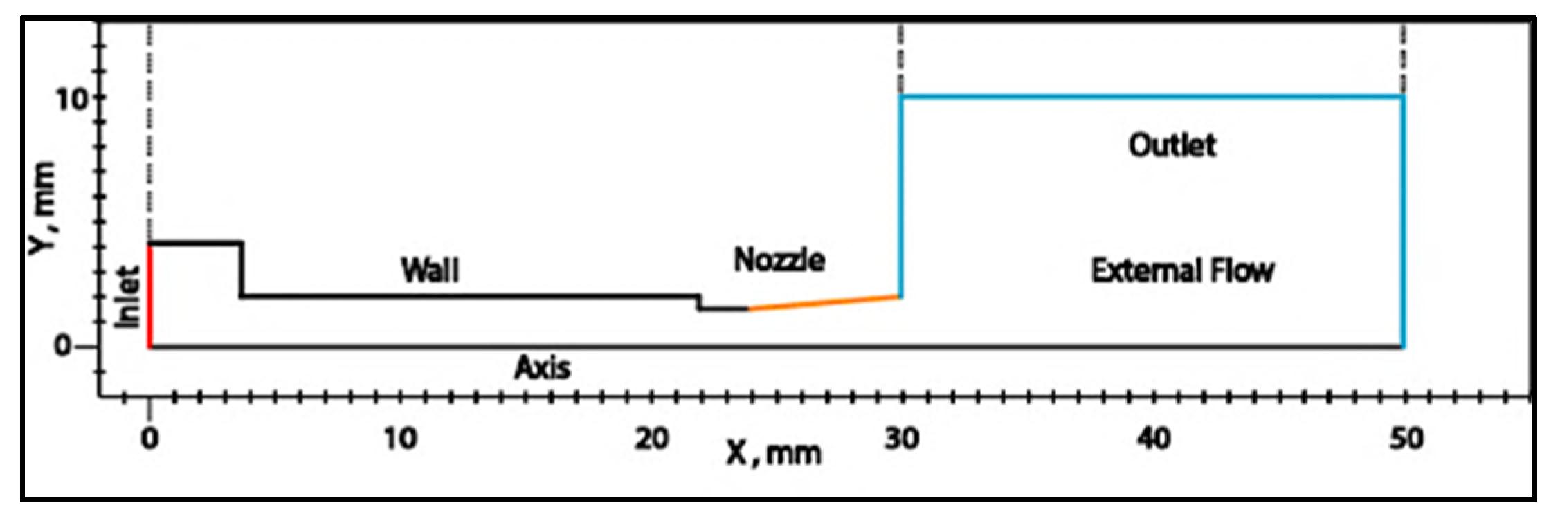
A geometry based on [3] was used, consisting of a rotational-symmetric 2D structure whose main objective is to reproduce the base shape of the injector. This model represents the injector’s dimensions in a simplified form. The two-dimensional rotating cross-section of the real model was used instead of the actual geometric model to simulate the symmetrical cylindrical nozzle. In Figure 3, the water flow entry can be seen traveling along the walls until it passes through the injector area, creating the cavitation phenomenon. Subsequently, the external flow at the outlet represents the water in a gaseous state. All dimensions are in millimeters. Similarly,

Table 1. Structure design of the two-dimensional injector.

Inlet Diameter	Inlet Length	Wall Diameter	Wall Length	Nozzle Diameter	Nozzle Length
2–4 mm	2–4 mm	4–6 mm	16–32 mm	0.5–2 mm	1–6 mm

shows the measurements used, which were the variables utilized in the SA algorithm: inlet diameter, inlet length, wall diameter, wall length, nozzle diameter, and nozzle length.

3.3. CFD Cavitation Model

The computational fluid dynamics (CFD) simulations were performed using Ansys^® Fluent 2020 R1 (Ansys^® Inc., Canonsburg, PA, USA), with the geometry and mesh setup conducted within the Ansys^® Workbench environment. To automate the simulation process, we utilized Journal mode in Fluent, which enables the scripting of simulation commands for sequential execution without manual intervention. This functionality allowed for consistent and repeatable simulation runs across multiple design configurations. The simulated annealing (SA) optimization algorithm was implemented in MATLAB R2022a (MathWorks Inc., Natick, MA, USA) using custom-developed scripts.

The simulations were performed on a laptop equipped with an Intel^® Core™ i5-9300H CPU @ 2.40 GHz, 32 GB of RAM, a 477 GB NVMe SSD, and an additional 894 GB SATA SSD. The system ran on a Windows 10 64-bit, and CFD simulations were executed using a NVIDIA GeForce GTX 1650 GPU with 4 GB of dedicated memory.

To represent the model in two dimensions, the previous geometry was used to delineate the model, which represents a section of the injector. Today, the Reynolds-averaged Navier–Stokes (RANS) model is a widely used turbulence model in industrial flow calculations due to its advantages in a broad range of applications, accuracy, and computational efficiency. Additionally, it has been demonstrated that the RNG k-ε model is effective in CFD cavitation analysis, providing the best results with minimal error. Therefore, this model was used to reproduce the cavitation behavior. The SIMPLEC algorithm and the finite volume method in Fluent were used to discretize the equations. Based on the Reynolds-averaged N–S equation, the momentum equation and the turbulent transport equation were discretized using the second-order upwind difference scheme, while the diffusion term was discretized using the central difference scheme. The pressure interpolation scheme for the continuity equation and the QUICK scheme for the convection term of the vapor volume fraction equation were employed by [23]. The inlet boundary condition of the nozzle was the pressure inlet with a pressure value of 4 MPa. The outlet boundary condition was fixed at zero pressure at the outlet. The nozzle boundary was set as a wall boundary condition (see

Table 2. Boundary conditions.

Pressure Inlet	Outlet	Walls	Turbulence Intensity	Reference Pressure
4 MPa	Fixed zero pressure	No-slip conditions for nozzle and wall	5% at inlet and outlet	0.101325 MPa

), and the geometric model axis was set as an axis boundary condition. The nozzle and wall were considered no-slip walls. The turbulence intensity of the jet at the inlet and outlet was set to 5%, and the reference pressure was 0.101325 MPa.

Water is presented as a mixture of two phases. In the first phase, it is liquid and has the characteristics shown in

Table 3. Water phases and properties.

Liquid Phase	Vapor Phase
Density (kg/m3)	Density (kg/m3)
998.2	0.5542
Viscosity (kg/m·s)	Viscosity (kg/m·s)
0.001003	1.34 × 10−5

. Similarly, the vapor phase displays the density and viscosity of the fluid, with a mass transfer mechanism from the liquid phase to the vapor phase through cavitation. This allows for a better observation of the areas where this phenomenon occurs, providing the volume fraction percentage of the mixture.

The cavitation phenomenon was modeled using the Zwart–Gerber–Belamri model implemented in Ansys Fluent, which simulates a two-phase mixture of liquid and vapor water. This model inherently includes the phase change process through mass transfer between the phases. Specifically, the model activates evaporation when the local pressure drops below the saturation vapor pressure of the liquid, and condensation when the pressure increases above it. Thus, a separate evaporation sub-model is not required, as these processes are intrinsically incorporated into the mass transfer mechanism defined by the cavitation model. This approach enables a more realistic prediction of the vapor volume fraction and the regions susceptible to cavitation within the flow domain.

3.4. Mesh

In this study, the computational domain was divided into blocks to create quadrilateral structured grids. A tetrahedral mesh was used, starting from the x-axis, to represent the calculation of the equations more precisely. The meshing process involved dividing the domain into small elements to accurately calculate the velocity, pressure, and density. Additionally, the mesh was refined in the injector area to better visualize the cavitation effect near the outlet. The main face of the model was selected for applying a standard mesh with an element size of 0.03 mm to represent the entire domain. Similarly, a refinement of 3 was applied to the sections of the geometry corresponding to the injector and the outlet angle. This resulted in 315,303 nodes and 312,287 elements for the reference geometry and 283,932 nodes and 281,755 elements for the optimized model geometry. In the same meshing area, zones were selected to input the boundary condition values, including the inlet, walls, and outlet, as shown in Figure 3.

3.5. SA Algorithm

In the simulated annealing (SA) algorithm [24], the author aimed to present an algorithm based on a reduction in the cost function, which was modified to utilize six different inputs and reduce each of the variables within the selected ranges. This, in combination with the Journal documents, allowed for the automatic opening and closing of the analysis program. Several parameters are crucial for its effective operation. The maximum number of iterations (MaxIt) determines how many times the main cycle of the algorithm will repeat, while the maximum number of sub-iterations (MaxSubIt) sets how many times an internal cycle can repeat within each main iteration. The initial temperature (T0) controls the probability of accepting worse solutions at the beginning to avoid falling into local optima, and the temperature reduction rate (alpha) defines how quickly the system cools, affecting the duration of exploration. The population size (nPop) indicates how many solutions are maintained and evaluated in each iteration, and the number of neighboring solutions (nMove) generated per current solution affects the breadth of the search. The mutation rate (mu) controls the probability of a solution being mutated, introducing variability to escape the local optima, while the mutation range (sigma) defines the magnitude of the changes introduced, influencing the precision and scope of the exploration. These parameters must be carefully adjusted to balance exploration and exploitation in the search for the optimal solution (see

Table 4. Parameters for the SA algorithm.

MaxIt	MaxSubIt	T0	Alpha	nPop	nMove	Mu	Sigma
40	1	0.01	0.9	4	2	0.2	0.1∗(VarMax − VarMin)

).

The algorithm mainly involves selecting the input geometry variables shown in Table 1, which follows the process outlined in the algorithm’s flowchart. These variables are used to calculate the initial solution of the cost function, which represents the percentage of volume fraction with random data within the selected ranges. Simultaneously, the initial variables were selected to calculate the initial temperature to start the algorithm’s cycle. The data were updated in a Journal file created in Ansys^®, which consists of the workflow for calculating the cavitation phenomenon through the aforementioned process, generating a solution for the percentage of cavitation.

The iteration cycle lasts for 3 days because the program runs the solution the same number of times as the product of the population size and the number of neighboring solutions generated. Once this transition between opening and closing the program is completed, an iteration is shown for calculating the cost function solution. The results obtained, once the solution criteria of the algorithm are met, must be evaluated to observe the reduction in the cavitation effect and make a comparison between the reference model and the new optimized model.

4. Results and Discussions

The results aimed to demonstrate the computational contribution of integrating Ansys^® with the simulated annealing (SA) algorithm for selecting and comparing the optimal geometric parameters in an improved injector model. Through this integration, it becomes possible to automate the evaluation of the volume fraction as the cost function, streamlining the comparison with a baseline model used as a reference. Additionally, a comparison of cavitation in the outlet region of the injector is presented to validate the effectiveness of the optimized geometry. Similarly, a comparison of output variables—specifically the operating pressure and velocity—is included, showing that the jet’s performance remained consistent despite the geometric changes.

4.1. Simulated Annealing Analysis

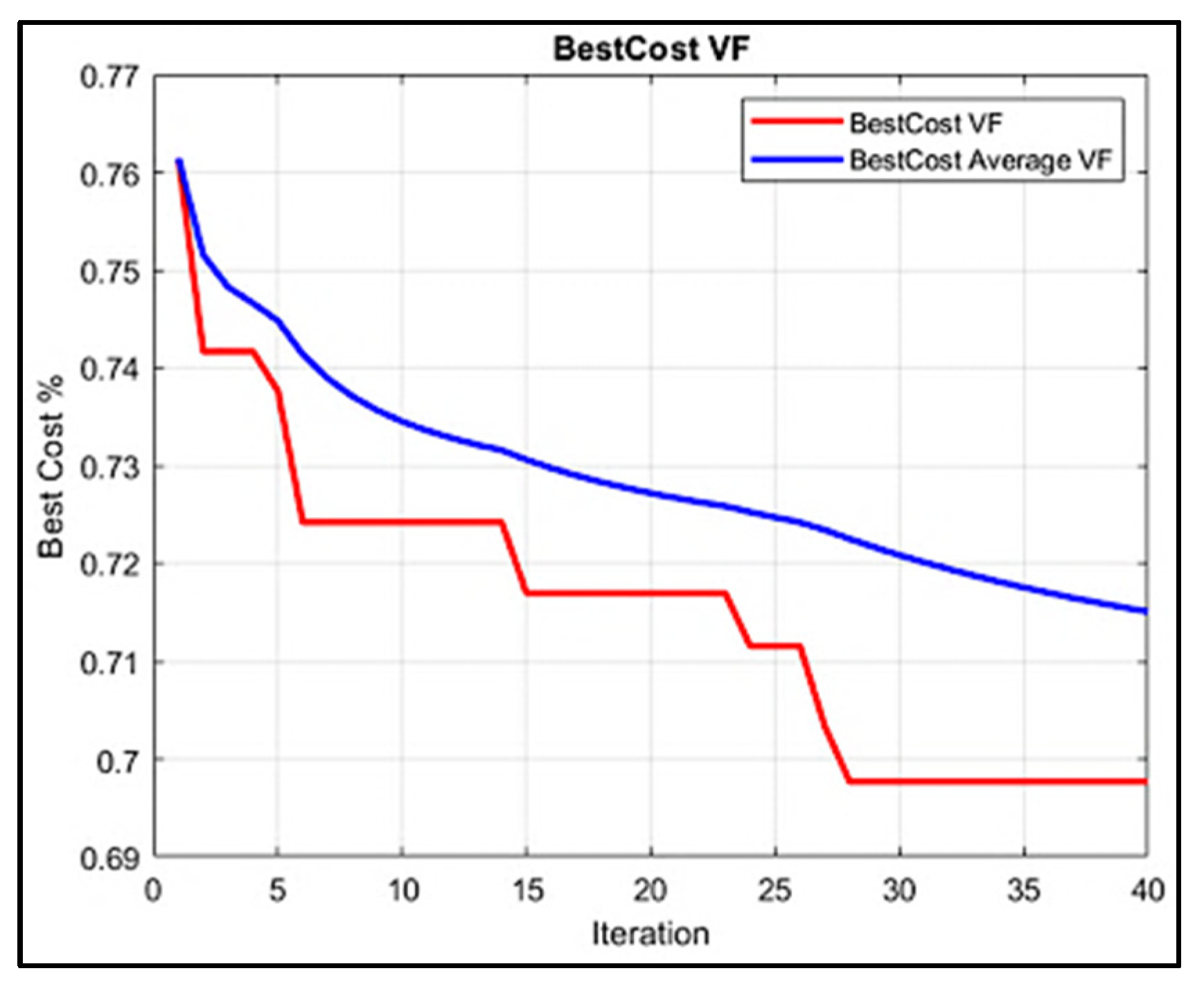
Figure 4 illustrates the evolution of iterations concerning the volume fraction calculation. The x-axis represents the number of iterations performed by the SA algorithm, which, in this case was 40. Meanwhile, the y-axis depicts the trend in cavitation percentage calculated for each iteration. Once the computation process concludes, the cost function data are analyzed, corresponding to the evaluation of each population element and its generated neighbors. The decreasing trend of the function can be observed iteration by iteration.

Initially, the cost function reduction trend per iteration is represented in red in Figure 4. It begins with random values based on the baseline model’s dimensions, with the first iteration yielding a volume fraction percentage of 76%. In contrast, the blue graph represents the average value of the same cost function, providing a more centralized reference. This function demonstrated a reduction in cost and temperature, ultimately reaching 69.2% for the optimized model. From iteration 27 onward, the volume fraction percentage calculation remained constant. Consequently, even if more than 40 iterations were performed, the results would stabilize, indicating that the algorithm performs reliably and that the model effectively reduces cavitation.

Geometric patterns were established to select the optimized variables, as the algorithm’s primary objective is to search for local minima and compare them until reaching a global minimum, ultimately determining the optimal model dimensions.

It is worth mentioning that the computational workload associated with the SA algorithm required 205,649.24 s to complete the selected 40 iterations. This execution was performed on a standard workstation, highlighting that the implementation of the algorithm does not necessitate access to high-performance computing resources. Nevertheless, the use of hardware with enhanced computational capabilities, such as multi-core processors, greater memory bandwidth, or GPU acceleration, would contribute to a substantial reduction in computational time, thereby increasing the overall efficiency of the optimization process. Similarly, the algorithm calculated the operations with the neighbors, resulting in 8 sub-iterations for each of the aforementioned iterations, generating 32 cycles in total, dividing each 8 cycles in each calculation of the main one. This work was carried out automatically with the implication that the algorithm might cycle and restart.

4.2. CFD-Based Volume Fraction Calculation

It was crucial to analyze the distribution of volume fraction zones in the CFD approximation model, as a comparative study of the phenomenon’s dispersion in the area of interest was conducted using input data from both the baseline and optimized models. As previously mentioned, the numerical process in Ansys^® estimated the fluid behavior in specific regions highlighted in red. In these areas, the fluid exhibited pressure drops at the injector outlet.

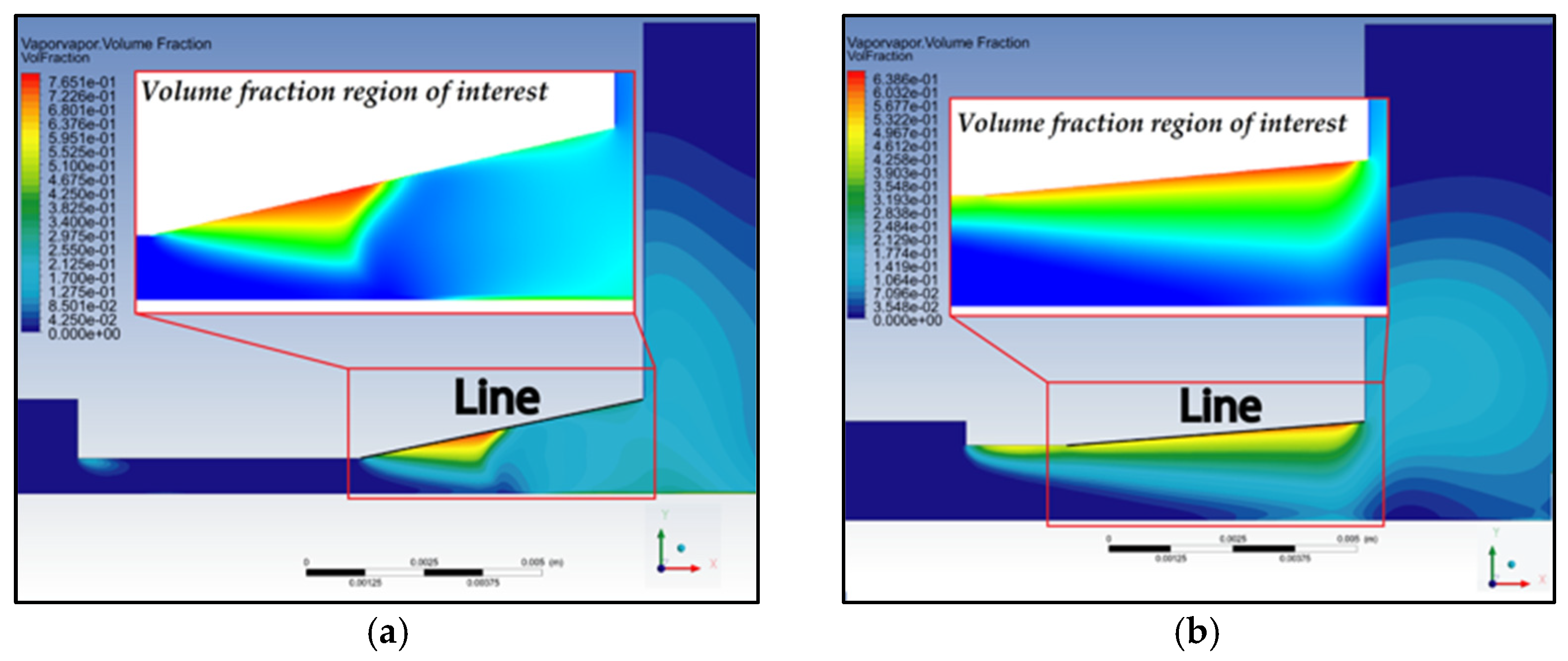
The results obtained for the baseline model are shown in Figure 5a, which illustrates the water flow at the injector outlet, yielding a volume fraction of 78.6%. The cavitation cloud was primarily concentrated at the outlet angle, indicating that this region is prone to cavitation-induced wear. The baseline geometry featured a small injector diameter of 0.75 mm and an extended length of 6 mm, leading to high negative pressure drops. Meanwhile, the velocity was calculated at approximately 65 m/s. To ensure proper cutting performance, the inlet and outlet pressures must be maintained similar to those of the baseline model.

In Figure 5b, the optimized model was constructed based on the dimensions calculated by the algorithm, featuring an injector diameter of 1.5145 mm and a length of 2.0225 mm. This modification caused the cavitation cloud to concentrate along the outlet angle, exhibiting lower values than the baseline model, with an estimated volume fraction of 65.9%. The optimized model was subsequently analyzed to evaluate the pressure and velocity behavior of the mixture, ensuring a fair comparison while maintaining the initial conditions. This approach aimed to preserve the operational characteristics of the cutting injector, similar to those used in [3].

Within the analysis program, it is possible to create an action line. Using the geometry sketch, an initial point with coordinates (x, y) and an endpoint with the same approach were established. This line had a length of 6 mm with a different angle. In the reference model, the cavitation behavior was observed in a specific area, and the line is denoted in black.

In Figure 5, it can be seen that the angle of the reference model (see Figure 5a) was larger, while the optimized model showed a line with the same length but at a smaller angle (see Figure 5b). This model will serve as a reference to establish a graph with cavitation data in both zones along the action line. The graphs generated with Ansys^® Fluent allowed for the establishment of contours to display the calculated results from the approximation processing for flow calculation.

In both subfigures of Figure 5, a zoomed-in section highlights the volume fraction region of interest, where the vapor phase distribution due to cavitation is clearly visible. The color map indicates the volume fraction of vapor, ranging from 0 (liquid) to values above 0.7 (mostly vapor), showing regions of phase change. The black line in each image was positioned across this region to collect and analyze the vapor volume fraction. Notably, the reference model (Figure 5a) presented a steeper inclination, while the optimized model (Figure 5b) had a gentler slope, resulting in a shift in the high vapor concentration zone. This difference in angle influenced the cavitation characteristics, which were quantitatively assessed through line plots derived from the data along these lines.

To explain the differences in vapor distribution observed in Figure 5, it is important to consider the geometric impact on flow behavior. The baseline model, with a narrower diameter and longer outlet length, generated higher velocities and a stronger pressure drop, resulting in a more concentrated cavitation cloud near the outlet (volume fraction of 78.6%). In contrast, the optimized geometry—wider and shorter—reduced the pressure losses and shifted the cavitation region upstream, leading to a lower vapor concentration (volume fraction of 65.9%) and a more diffused distribution. The difference in outlet angle also contributed to this shift. To support this analysis, a common action line was used in both models to extract the volume fraction data, as shown in Figure 6. The baseline showed a sharp peak in cavitation, while the optimized model displayed a smoother curve, confirming a reduced cavitation intensity due to the geometric improvements.

4.3. Volume Fraction Distribution on the Action Line

The tabulated data for both analyses show the behavior of the cavitation cloud along the action line, and the results can be seen in Figure 6. The red dotted line shows the percentage of the volume fraction along the axis established at the outlet angle of the base model, with data above a 70% concentration and a peak at 43.8 mm along the x-axis, followed by a decrease in occurrence at 45 mm. In contrast, the blue graph showed an almost linear behavior of cavitation occurrence with a maximum of 63%, generating a lower concentration cloud in the optimized design and decreasing sharply once the mixture exit the system in a gaseous state, representing the result as atomization. Similarly, the action line measured 6 mm in both cases, but for the optimized model, the overall geometry length was reduced, with the highest concentration occurring between 23 mm and 30 mm.

4.4. Pressure

Another key factor to consider is the pressure distribution and how it varies when comparing the baseline model to the optimized one, as this allows for the evaluation of the proper functioning of both designs. It is important to emphasize that the inlet and outlet pressures must remain stable. Below, a comparison is presented between the pressure values calculated for each model: the reference model and the optimized model, whose geometry was determined using the simulated annealing (SA) algorithm.

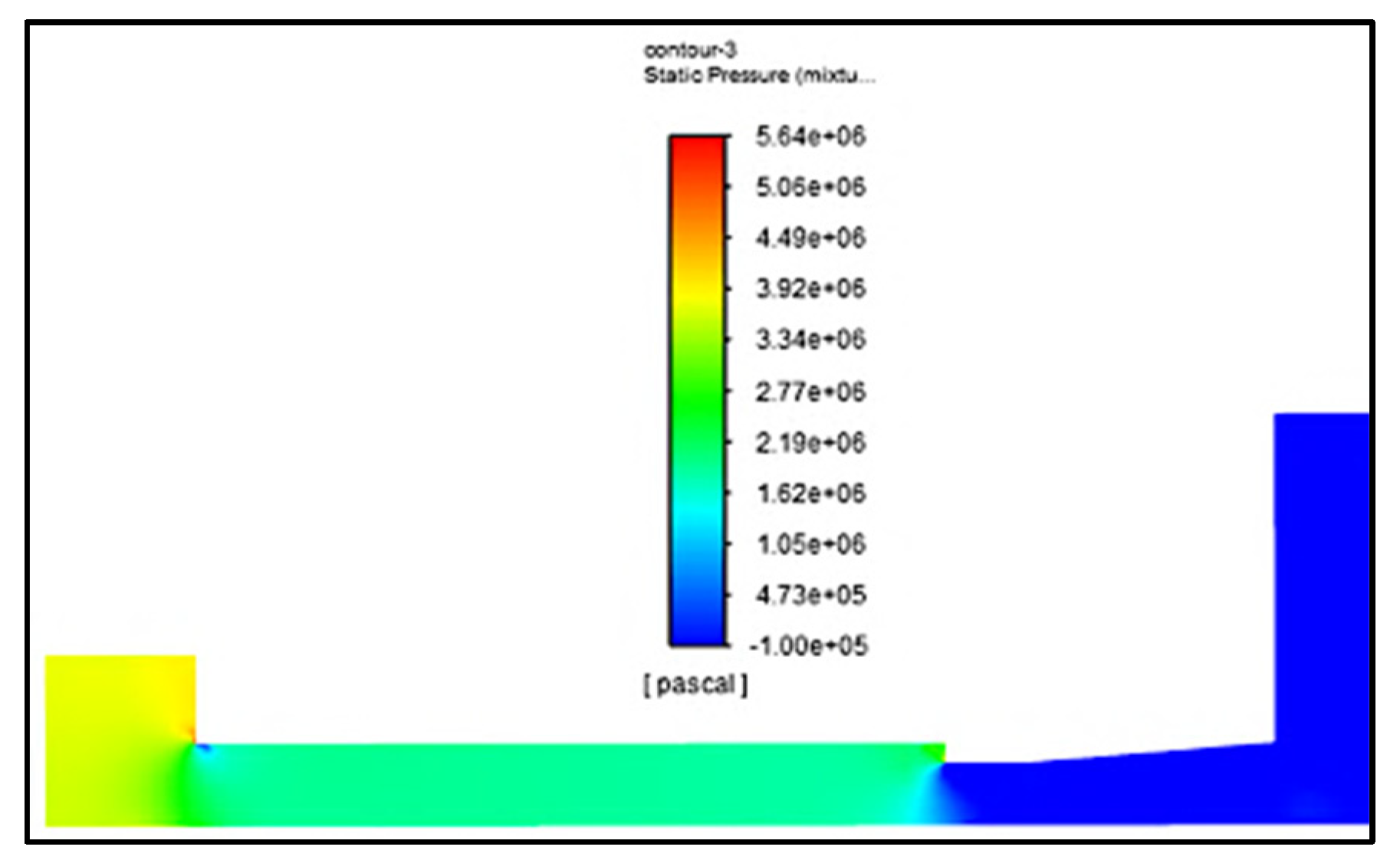
In comparison with the baseline model, the system pressure remained stable in the optimized configuration. The optimized geometry showed an inlet pressure of 4 MPa and an outlet pressure of 0 MPa. Pressure peaks of up to 5.6 MPa appeared at specific vertices due to turbulence generated by the geometry. The blue regions indicated pressure drops, which corresponded to the primary zones where cavitation occurred. Figure 7 illustrates a pressure contour along the geometry, showing the fluid behavior up to the outlet. A clear pressure drop was observed near the outlet, which coincided with the phase change zone—from liquid to vapor—where the RANS equations captured both the pressure variation and the appearance of the volume fraction.

The baseline model exhibited less variation in pressure compared with the optimized model, showing an inlet pressure of 6 MPa that also dropped to 0 MPa at the outlet. The optimized model, therefore, maintained suitable pressure characteristics for system operation, comparable to those of the baseline design.

4.5. Velocity

Similarly, when optimizing the model, it is important to clarify that the liquid velocity must remain comparable to that of the baseline model. A significant drop in velocity must be avoided, as it would compromise the primary function of the cutting jet, rendering it ineffective for the intended operational range.

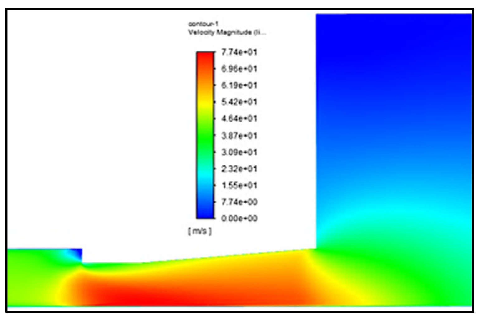
In this regard, the reference model initially yielded a maximum outlet velocity of 65.3 m/s. After applying the computational procedure with the optimized parameters, it was observed in Figure 8 that the velocity increased at the outlet, reaching up to 77.4 m/s. As previously discussed, although the pressure decreases, this benefits the outlet by enhancing the velocity. Consequently, the performance of the cavitating injector improves at the outlet, which is critical given that these injectors are primarily used for material-cutting applications. The optimized geometry thus enhances the outlet behavior by facilitating a more effective mixture of the liquid and vapor phases of water.

5. Conclusions

This study presented a computational strategy for optimizing the geometry of a water jet injector through the integration of CFD analysis and the simulated annealing (SA) algorithm. The primary objective was to minimize cavitation at the injector outlet without compromising key performance variables such as pressure and velocity. Beginning with a reference model, the initial CFD simulations revealed a cavitation volume fraction of approximately 80%. By applying the SA algorithm, the volume fraction was reduced to 65.9%, all while maintaining the inlet pressure at 4 MPa and improving the outlet velocity from 65.3 m/s to 77.4 m/s—favorable for high-velocity jet cutting applications.

A key component of this work was the integration of Ansys^® Journal mode with MATLAB. Journal mode enables the automation of parametric updates, batch execution of numerical analyses, and efficient management of input/output data through scripting. When combined with MATLAB, it allows for the real-time modification of design variables, automatic execution of the analysis workflow, and seamless integration with the optimization algorithm. This reduces human error, accelerates the design cycle, and enables high-throughput numerical studies.

The MATLAB code dynamically adjusts geometry inputs and writes them into Journal files that Ansys^® Workbench reads to perform CFD simulations. The resulting volume fraction, pressure, and velocity data are then automatically extracted and evaluated by the algorithm to update the cost function. This iterative feedback loop continues for several days, representing hundreds of iterations, and leads to the successful identification of an optimal injector configuration.

The robustness of this automated framework lies in its ability to explore the design space effectively, reduce computational effort, and deliver stable, optimized results. The convergence of the cost function throughout the iterations confirmed the consistency of the solution, while graphical analyses supported the algorithm’s ability to escape the local minima and find a global optimum.

Beyond the specific case of cavitation reduction in injectors, the methodology is applicable to a wide range of fluid–structure interaction problems. It can be adapted to optimize heat exchangers, nozzles, pumps, or biomedical devices—any system where geometric parameters significantly influence performance. Moreover, the proposed integration streamlines the design-to-validation pipeline, offering a valuable tool for researchers and engineers aiming to enhance performance through automated computational design.

In conclusion, the proposed framework not only improves the design quality and performance of cavitating injectors, but also opens up a path for scalable, automated optimization methods in advanced engineering applications. This work sets the stage for future experimental validations, rapid prototyping, and deployment in industrial systems requiring high-efficiency, fluid-based solutions.

References

- Yu-Kang, Z.; Jiu-Gen, H.; Hammitt, F.G. Cavitation erosion of cast iron diesel engine liners. Wear 1982, 76, 329–333. [Google Scholar] [CrossRef]
- Brunhart, M.; Soteriou, C.; Daveau, C.; Gavaises, E.; Koukouvinis, P.; Winterbourn, M. Investigation on the removal of the cavitation erosion risk in a control orifice inside a prototype diesel injector. In Proceedings of the Fuel Systems—Engines, London, UK, 4–5 December 2019. [Google Scholar]
- Wu, X.Y.; Zhang, Y.Q.; Tan, Y.W.; Li, G.S.; Peng, K.W.; Zhang, B. Flow-visualization and numerical investigation on the optimum design of cavitating jet nozzle. Pet. Sci. 2022, 19, 2284–2296. [Google Scholar] [CrossRef]
- Saha, K. Modelling of Cavitation in Nozzles for Diesel Injection Applications. Ph.D. Thesis, University of Waterloo, Waterloo, ON, Canada, 2014. [Google Scholar]
- Zeidi, S.M.J.; Mahdi, M. Effects of nozzle geometry and fuel characteristics on cavitation phenomena in injection nozzles. In Proceedings of the 22st Annual International Conference on Mechanical Engineering-ISME, Ahvaz, Iran, 22 April 2014. [Google Scholar]
- Giannadakis, E.; Gavaises, M.; Arcoumanis, C. Modelling of cavitation in diesel injector nozzles. J. Fluid Mech. 2008, 616, 153–193. [Google Scholar] [CrossRef]
- He, Z.; Zhong, W.; Wang, Q.; Jiang, Z.; Shao, Z. Effect of nozzle geometrical and dynamic factors on cavitating and turbulent flow in a diesel multi-hole injector nozzle. Int. J. Therm. Sci. 2013, 70, 132–143. [Google Scholar] [CrossRef]
- Mouvanal, S.; Chatterjee, D.; Bakshi, S.; Burkhardt, A.; Mohr, V. Numerical prediction of potential cavitation erosion in fuel injectors. Int. J. Multiph. Flow 2018, 104, 113–124. [Google Scholar] [CrossRef]
- Payri, R.; Margot, X.; Salvador, F.J. A Numerical Study of the Influence of Diesel Nozzle Geometry on the Inner Cavitating Flow (No. 2002-01-0215); SAE Technical Paper: Warrendale, PA, USA, 2002. [Google Scholar]
- Li, W.; Li, E.; Shi, W.; Li, W.; Xu, X. Numerical simulation of cavitation performance in engine cooling water pump based on a corrected cavitation model. Processes 2020, 8, 278. [Google Scholar] [CrossRef]
- Yu, Y.; Shademan, M.; Barron, R.M.; Balachandar, R. CFD study of effects of geometry variations on flow in a nozzle. Eng. Appl. Comput. Fluid Mech. 2012, 6, 412–425. [Google Scholar] [CrossRef]
- Arora, J.S. Introduction to Optimum Design; Elsevier: Amsterdam, The Netherlands, 2004. [Google Scholar]
- Moins, S. Implementation of a Simulated Annealing Algorithm for Matlab. Available online: https://www.diva-portal.org/smash/record.jsf?pid=diva2%3A18667&dswid=8349 (accessed on 30 April 2025).
- Stern, J.M. Simulated annealing with a temperature dependent penalty function. ORSA J. Comput. 1992, 4, 311–319. [Google Scholar] [CrossRef]
- Guilmeau, T.; Chouzenoux, E.; Elvira, V. Simulated annealing: A review and a new scheme. In Proceedings of the 2021 IEEE Statistical Signal Processing Workshop (SSP), Rio de Janeiro, Brazil, 11–14 July 2021; pp. 101–105. [Google Scholar]
- Becerra, R.L.; Coello, C.A.C. Cultured differential evolution for constrained optimization. Comput. Methods Appl. Mech. Eng. 2006, 195, 4303–4322. [Google Scholar] [CrossRef]
- Tu, J.; Yeoh, G.H.; Liu, C. Computational Fluid Dynamics: A Practical Approach; Butterworth-Heinemann: Oxford, UK, 2018. [Google Scholar]
- Cortés Rivera, D.; Landa Becerra, R.; Coello Coello, C.A. Cultural algorithms, an alternative heuristic to solve the job shop scheduling problem. Eng. Optim. 2007, 39, 69–85. [Google Scholar] [CrossRef]
- Kirkpatrick, S.; Gelatt, C.D., Jr.; Vecchi, M.P. Optimization by simulated annealing. Science 1983, 220, 671–680. [Google Scholar] [CrossRef] [PubMed]
- Aarts, E.; Korst, J. Simulated Annealing and Boltzmann Machines: A Stochastic Approach to Combinatorial Optimization and Neural Computing; John Wiley & Sons, Inc.: Hoboken, NJ, USA, 1989. [Google Scholar]
- Van Laarhoven, P.J.; Aarts, E.H.; van Laarhoven, P.J.; Aarts, E.H. Simulated Annealing; Springer: Berlin/Heidelberg, Germany, 1987; pp. 7–15. [Google Scholar]
- Ramalingam, S.; Subramanian, R.A. Solving level scheduling in mixed model assembly line by simulated annealing method. Circuits Syst. 2016, 7, 907. [Google Scholar] [CrossRef]
- Matsson, J.E. An Introduction to Ansys® Fluent 2022; Sdc Publications: Mission, KS, USA, 2022. [Google Scholar]
- Mostapha Kalami Heris, Real-Coded Simulated Annealing (SA) in MATLAB. Yarpiz. 2015. Available online: https://yarpiz.com/421/ypea106-real-coded-simulated-annealing (accessed on 31 July 2023).