On Generating Synthetic Datasets for Photometric Stereo Applications

Abstract

The mathematical model for photometric stereo makes several restricting assumptions, which are often not fulfilled in real-life applications. Specifically, an object surface does not always satisfies Lambert’s cosine law, leading to reflection issues. Moreover, the camera and the light source, in some situations, have to be placed at a close distance from the target, rather than at infinite distance from it. When studying algorithms for these complex situations, it is extremely useful to have at disposal synthetic datasets with known exact solutions, to assert the accuracy of a solution method. The aim of this paper is to present a Matlab package which constructs such datasets on the basis of a chosen exact solution, providing a tool for simulating various real camera/light configurations. This package, starting from the mathematical expression of a surface, or from a discrete sampling, allows the user to build a set of images matching a particular light configuration. Setting various parameters makes it possible to simulate different scenarios, which can be used to investigate the performance of reconstruction algorithms in several situations and test their response to lack of ideality in data. The ability to construct large datasets is particularly useful to train machine learning based algorithms.

1. Introduction

Computer vision techniques find application in many different fields. Among these, the digital reconstruction of objects is an extensively studied topic, for which various mathematical models are available. The idea behind Shape from Shading (SfS) is to derive shape and color information from a single image of the object [1,2,3]. Since this problem is ill-posed, an alternative SfS technique denoted photometric stereo (PS) [4,5] is often used to determine the three-dimensional shape of an observed target from a set of images. The original formulation requires that images are obtained by light sources placed at different known positions, theoretically at infinite distance from the target, and that the object surface is Lambertian. Under these assumptions, it was proved by Kozera [6] that for the problem to have a unique solution at least two images with different lighting must be available. In this case, the solution method is based on the resolution of a system of first-order Hamilton-Jacobi partial differential equations, which have been studied by different numerical approaches; see, e.g., [7]. However, the assumptions of the model are very limiting, especially in real-life applications.

In [8], PS was applied to an archaeological scenario, with the aim of reconstructing the digital shape of rock art carvings found in various sites; see, e.g., [9]. In this kind of applications, light source has often to be placed close to the surface, due to the structure of the excavation sites. For similar light configurations different methods have been developed, including learning-based models as those presented in [10,11]. An additional issue in archaeology is that the rock is not an ideal Lambertian reflector. This condition have been largely studied using different algorithmic approaches: some based on a statistical model [12], others on learning-based methods [13,14,15,16]. A pre-processing of non-Lambertian data has been discussed in [17], while in [8] a method to extract from dataset a subset of pictures which satisfy the ideal assumptions of the model has been introduced.

Various benchmark datasets for PS are available: some are obtained from real objects [18,19,20,21], some are synthetic datasets, as CyclePS [22], PSWild [23], and PSMix [24], built from online 3D models, for which different reflectance functions have been chosen to replicate real objects. In [25], the Blobby Shape Dataset was presented. This synthetic dataset is obtained by considering 10 fixed surfaces in 10 lighting environments, with a physically-based renderer. A software package to construct a dataset of 100 images of these surfaces, under fixed lighting conditions, is available.

The aim of this paper is to present a Matlab package which allows the user to construct arbitrarily large synthetic datasets that reflect particular observation conditions, starting from a chosen model surface, either known by its mathematical representation or by a discrete sampling. A limited choice of symbolic surfaces is available in the package, but its number can be easily extended. The user can choose the number of light sources and their position, and the package deals with two deviations from the standard Lambertian model: the “close-light configuration”, which allows the user to position selected light sources at a finite distance from the observed object, and the reflection phenomenon, that is, the possibility for the surface to reflect light specularly. Setting specific parameters, the user can produce datasets which combine such issues. Differently from available datasets, where the observation conditions are fixed, with our tool one can freely choose the scenario configuration and generate as many “pictures” as needed, by suitable changing some parameters. Two demonstration programs show how to use the package to produce datasets with different features.

Our study is not oriented to a particular reconstruction method, but produces general datasets that can be used to ascertain the performance of any method, by comparing the results with the exact solution.

The paper is organized as follows: in Section 2 we resume the photometric stereo mathematical model. Section 3 describes the algebraic setting for generating datasets with lights at a finite distance, while Section 4 shows how we deal with reflective surfaces. The software implementation and its use are discussed in Section 5, where some example datasets are also displayed. A sensitivity analysis for datasets produced by the package is performed in Section 6, where an example of its use as a data generator for reconstruction algorithms is also illustrated. Section 7 contains final considerations.

2. The Mathematical Model for Photometric Stereo

In this section we briefly review the mathematical setting introduced in [5], with the notation adopted in [26].

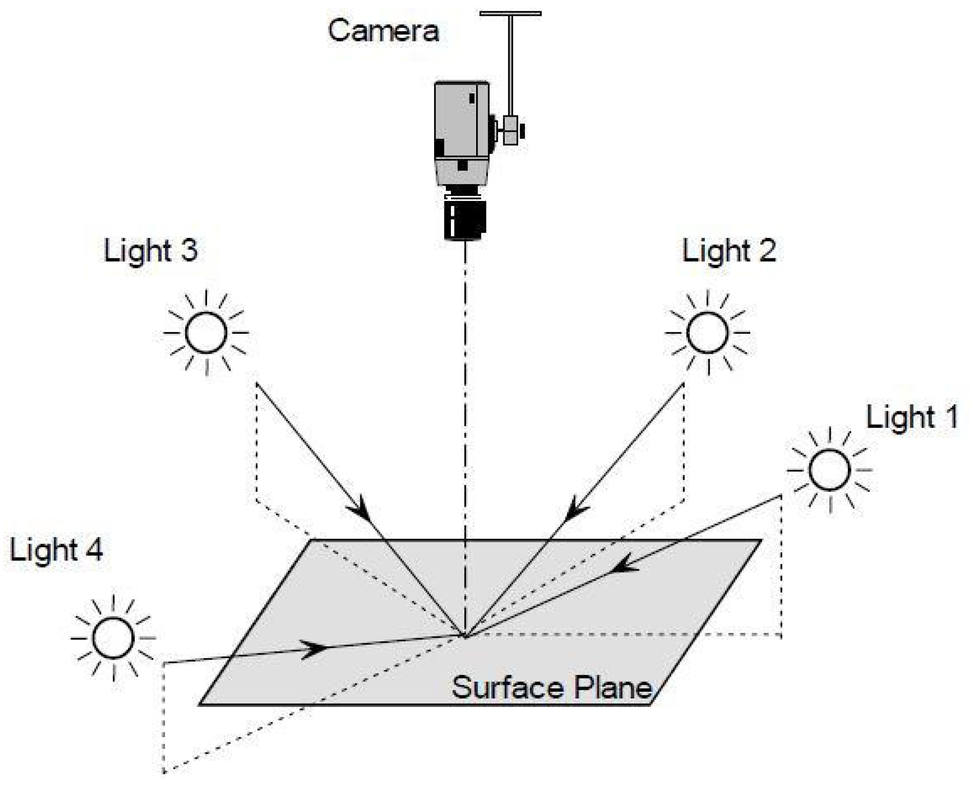
The photometric stereo (PS) technique provides the reconstruction of object surfaces on the basis of information contained in a set of digital pictures. The camera position is theoretically fixed at infinite distance from the object, and the light source is positioned far from the object at different directions, which are assumed to be known, in order to obtain images under different lighting conditions; see Figure 1. The assumption of infinite distance from the target for both the camera and the light sources implies that orthographic projection can be used to describe the scene and that the light rays are all parallel to a fixed vector, different for each picture.

A reference system is fixed in ${\mathbb{R}}^3$, so that the observed object is located at the origin and the optical axis of the camera coincides with the z-axis. Each image has resolution $(r+2)\times (s+2)$, and is associated to a rectangular domain $\mathsf{\Omega }=\left[-{\displaystyle \frac{A}{2}},{\displaystyle \frac{A}{2}}\right]\times \left[-{\displaystyle \frac{B}{2}},{\displaystyle \frac{B}{2}}\right]$, where A is the horizontal size of the image and $B=(s+1)h$ is its vertical size, with $h=A/(r+1)$.

If the surface is represented by the bivariate function $z=u(x,y),(x,y)\in \mathsf{\Omega }$, the normalized normal vector can be expressed as

$$\mathbf{n}(x,y)={\displaystyle \frac{{[-u_x,-u_y,1]}^T}{\sqrt{1+{\parallel \nabla u\parallel }^2}}},$$

(1)

where $u_x$, $u_y$ denote the partial derivatives of u, $\nabla u$ its gradient, and $\parallel ·\parallel$ the 2-norm.

We consider a discretization of the domain, i.e., a grid of points with coordinates $(x_i,y_j)$, $i=0,\dots ,r+1$, $j=0,\dots ,s+1$, and we sort the pixels lexicographically. Then, the symbols $u(x_i,y_j)$, $u_{i,j}$, $u_k$, indifferently represent the value assumed by u at the points of the grid, where $k:=(i-1)s+j=1,\dots ,p$ indexes the internal points and $p=rs$ represents their number.

Assuming that q images are available, the vector that spreads from the object to the light source is denoted by ${\mathsf{\ell }}_t={[{\mathsf{\ell }}_{1,t},{\mathsf{\ell }}_{2,t},{\mathsf{\ell }}_{3,t}]}^T$, $t=1,\dots ,q$. Its norm is chosen proportional to the light intensity

Saying that the surface of the object is a Lambertian reflector means that it satisfies Lambert’s cosine law

$$\rho (x,y)\langle \mathbf{n}(x,y),{\mathsf{\ell }}_t\rangle =I_t(x,y),t=1,\dots ,q,$$

(2)

where the albedo $\rho (x,y)$ represents the partial absorption of the light at each point of the surface and $I_t(x,y)$ is the perceived light intensity, that is, the pixel value at the point $(x,y)$ of the tth image.

By discretizing Formula (2) and ordering pixels lexicographically, Lambert’s law can be expressed in the matrix form as

$$D{N}^{T}L=M.$$

(3)

In this expression, $D=\mathrm{diag}({\rho }_1,\dots ,{\rho }_p)$, where ${\rho }_k$, $k=1,\dots ,p$, is the albedo at the internal points, $N=[{\mathbf{n}}_1,\dots ,{\mathbf{n}}_p]$ and $L=[{\mathsf{\ell }}_1,\dots ,{\mathsf{\ell }}_q]$ contain respectively the normal vectors and the lighting directions, and the tth column of $M=[{\mathbf{m}}_1,\dots ,{\mathbf{m}}_q]$ represents the vectorized image $I_t$ of the dataset.

The standard PS formulation assumes the knowledge of lighting positions, i.e., the matrix L. Then, the solution can be easily found by setting $\tilde{N}=ND$ and computing $\tilde{N}=M{L}^{†}$, with $L^{†}$ the pseudoinverse matrix of L [27]. By normalizing the columns of $\tilde{N}$ one finds an approximation of the normal vector field N and the albedo matrix D. Finally, the solution of the Poisson problem $\Delta u(x,y)=f(x,y)$, where f is obtained by numerically differentiating the normal field, provides the surface of the object; see [8] for details.

In some applications, the request for known lighting is a huge limitation, as it might be rather difficult to detect the exact position of the light source during the acquisition of the images. In [26], a method to solve the photometric stereo problem under unknown lighting was analyzed, based on Hayakawa’s procedure for unknown lighting PS [28]. Other approaches for light localization have been considered; see, e.g., [29].

In this paper, we will use Equation (3) as a direct model to generate the data matrix M, given the position of the light sources, a continuous or discrete representation of the surface, and its albedo. If the continuous representation is chosen, than the functions u, $u_x$, and $u_y$ must be supplied. If one prefers a discrete representation, the coordinates $(x_i,y_i,z_i$), $i=1,\dots ,p$, of each point of the surface are needed. In this case, the partial derivatives $u_x$ and $u_y$ are approximated by second order finite differences. The albedo can be either a grayscale image, or a RGB color image.

This model only approximates real observation scenes. Indeed, many studies showed that some of its assumptions are not met in experimental settings. As remarked in [8], the request on the light position is particularly limiting in archaeological applications, since several sites do not allow to position the light sources at sufficient distance from the target.

Also, real-world surfaces rarely satisfy Lambert’s law, causing distortions in collected data. Differently from the Lambertian case, whose model is discussed in this section, there is not a general model for non-Lambertian surfaces, so the available reconstruction approaches generally consider specific aspects of non-Lambertianity.

Designing algorithms that can handle these situations require the availability of realistic datasets reproducing specific scene configurations. Synthetic datasets has the advantage to allow a developer to test an algorithm performance by comparing the reconstructed solution with the exact object which generated the data.

In the next two section we focus on two particular situations, namely, “close-lights” and reflection, which have already been discussed in the Introduction and are quite common in real-world applications. The aim is to provide reliable datasets for testing the performance of reconstruction algorithms.

3. The Case of Close Lights

When a light is positioned at a finite distance from the observation, every point of the surface is illuminated from a different direction, as light rays diverge from the source. If we denote by ${\mathbf{v}}_j$ the position vector of the jth point of the surface, then the relative position of the ith light from that point is ${\mathsf{\ell }}_i-{\mathbf{v}}_j$, for $i=1,\dots ,q$ and $j=1,\dots ,p$. The light intensity is damped from an attenuation factor ${\delta }_{i,j}$, which depends on the distance between the illuminated point and the light source. Its theoretical value is ${\delta }_{i,j}={\parallel {\mathsf{\ell }}_i-{\mathbf{v}}_j\parallel }^{-2}$, but it is often chosen as ${\delta }_{i,j}={\parallel {\mathsf{\ell }}_i-{\mathbf{v}}_j\parallel }^{-1}$; see Section 9.7 from [30]. Our software allows the adoption of both values.

With this notation, the light intensity produced by the ith light at the jth point is given by

$$m_{j,i}={\rho }_j{\mathbf{n}}_j^T{\tilde{\mathsf{\ell }}}_{i,j},$$

(4)

where ${\tilde{\mathsf{\ell }}}_{i,j}={\delta }_{i,j}({\mathsf{\ell }}_i-{\mathbf{v}}_j)$; $m_{j,i}$ represents the jth pixel value of the ith image.

To obtain an efficient algorithm for the generation of a synthetic dataset, we express the computation in matrix form. Let us first consider the block-diagonal matrix

$$N_s=\left[\begin{array}{c}{\mathbf{n}}_1\\ & {\mathbf{n}}_2\\ & & \ddots \\ & & & {\mathbf{n}}_p\end{array}\right]\in {\mathbb{R}}^{\left(3p\right)\times p}.$$

Even if its size is quite large, it can be efficiently created as a sparse matrix, which requires a storage space slightly larger than the original matrix N.

We gather the position vectors of the surface points in the matrix

$$W=[{\mathbf{v}}_1,\dots ,{\mathbf{v}}_p],$$

and define, for $i=1,\dots ,q$,

$$V_i=({\mathsf{\ell }}_i{\mathbf{u}}_p^T-W){\Delta }_i=[{\mathsf{\ell }}_i-{\mathbf{v}}_1,\dots ,{\mathsf{\ell }}_i-{\mathbf{v}}_p]{\Delta }_i,$$

with ${\mathbf{u}}_p={(1,\dots ,1)}^T\in {\mathbb{R}}^p$ and ${\Delta }_i=\mathrm{diag}({\delta }_{i,1},\dots ,{\delta }_{i,p})$. The matrix $V_i$ contains the vectors joining each surface point to the ith light source, damped by the attenuation factors ${\delta }_{i,j}$.

We vectorize each $V_i$ in lexicographic order in the matrix

$$V=[\mathrm{vec}\left(V_1\right),\dots ,\mathrm{vec}\left(V_q\right)].$$

It is then immediate to verify that Equation (4) gives the generic entry of the matrix M defined by

$$M=D{N}_s^{T}V,$$

(5)

where D is the diagonal albedo matrix. Equation (5) allows for a fast and efficient construction of the dataset corresponding to a PS scenario with lights at a finite distance.

4. The Reflection Phenomenon

The basic property of Lambertian surfaces is that they diffuse light in the same way in every direction, i.e., their brightness does not depend on the point of view. This describes a class of ideal Lambertian reflectors which includes few real surfaces: actually, the majority of existing objects present characteristics for which Lambert’s law is not satisfied.

Non-ideal reflectors are such that the brightness at each point depends on the viewing angle. For this reason, some of them may present the phenomenon of reflection, which leads to distortion in the ideal PS data.

This phenomenon implies that, when the reflected light ray is parallel to the optical axis of the camera, the corresponding point presents a lighting intensity much larger than expected according to the PS model, leading to errors in the reconstruction.

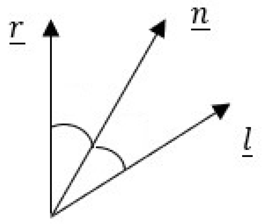
Since for each pixel the angle between the normal vector $\mathbf{n}$ and the lighting vector ℓ is equal to the one between $\mathbf{n}$ and the reflected vector $\mathbf{r}$, as in Figure 2, reflection occurs when $\mathbf{r}$ is parallel to the optical axis of the camera, that is, the z axis.

Starting from this consideration, using elementary geometric notions, the reflected vector at the point j of the ith image is given by

$${\mathbf{r}}_j^{\left(i\right)}=2\left({\mathbf{n}}_j^T{\mathsf{\ell }}_i\right){\mathbf{n}}_j-{\mathsf{\ell }}_i,i=1,\dots ,q,j=1,\dots ,p.$$

The above relation can be expressed in the following matrix form

$$R_i=N\mathrm{diag}\left(2N^T{\mathsf{\ell }}_i\right)-{\mathsf{\ell }}_i{\mathbf{u}}_p^T,$$

(6)

where $R_i=[{\mathbf{r}}_1^{\left(i\right)},\dots ,{\mathbf{r}}_p^{\left(i\right)}]$ and ${\mathbf{u}}_p={(1,\dots ,1)}^T\in {\mathbb{R}}^p$.

Reflection occurs at the jth point when the angle ${\theta }_j^{\left(i\right)}$ between ${\mathbf{r}}_j^{\left(i\right)}$ and the vector $\mathbf{z}={[0,0,1]}^T$ is equal to zero. For detecting such situation, we consider

$$\cos {\theta }_j^{\left(i\right)}={\displaystyle \frac{\langle {\mathbf{r}}_j^{\left(i\right)},\mathbf{z}\rangle }{\parallel {\mathbf{r}}_j^{\left(i\right)}\parallel \parallel \mathbf{z}\parallel }}={\displaystyle \frac{{\left({\mathbf{r}}_j^{\left(i\right)}\right)}_3}{\parallel {\mathbf{r}}_j^{\left(i\right)}\parallel }},$$

where ${\left({\mathbf{r}}_j^{\left(i\right)}\right)}_3$ is the third component of the reflected vector.

To construct a new dataset $\tilde{M}$ which keeps into account reflection, we modify a given dataset M by the simple rule

$${\tilde{m}}_{i,j}=\left\{\begin{array}{cc}max(m_{i,j},{\kappa }_R),\hfill & \mathrm{if}\arccos {\theta }_j^{\left(i\right)}<{\tau }_R,\hfill \\ m_{i,j},\hfill & \mathrm{otherwise},\hfill \end{array}\right.$$

(7)

where ${\tau }_R$ is a chosen tolerance, and ${\kappa }_R$ the pixel value which characterizes reflection for the given surface. Setting a value of ${\tau }_R$ significantly larger than zero results in a wide reflecting area in the neighborhood of the reflection point. The choice of ${\kappa }_R$ may be useful to specify different surface materials.

When the lights are positioned at a finite distance from the target, the computation in (6) is suitably modified according to the notation used in Section 3.

5. Software Description

This section describes a Matlab software (developed on version R2024b) to generate synthetic datasets for the photometric stereo problem. It can manage different PS configurations: the ideal one, the case of lights at finite distance, and the case of reflecting surfaces.

The psdatasynth Matlab package is available at the web page https://bugs.unica.it/cana/software.html (accessed on 27 April 2025). It consists of 6 functions and 2 demonstration scripts, listed in

Table 1. Functions of the psdatasynth package.

psdatagen	Demo program to illustrate the use of the package.
makepsimages	Generate a synthetic dataset based on a chosen configuration.
choosefun	Return symbolic descriptions of 5 test surfaces.
makealbedo	Create the albedo matrix D.
createlights	Create the matrix containing the light source directions.
plotlights3d	Plot the light directions.
psimshow	Display images with chosen resize factor and color limits.
genbigdataset	Demo program to create a large dataset

.

The demo program psdatagen shows how to set various parameters and call the other routines. The function makepsimages is the one that actually constructs the synthetic dataset by generating the matrix M starting from a chosen surface. The surface may be a symbolic function, selected by the choosefun, or a discretized one. The albedo matrix D is constructed by the makealbedo function. Both functions may be easily extended to add more symbolic surfaces and albedo types to the package.

The remaining functions are createlights, which constructs the light matrix L, and the visualization functions plotlights3d and psimshow. The last two functions are used internally and will rarely be called directly by the user.

The functions choosefun, createlights, makealbedo, and plotlights3d, were included without documentation in the ps3d Matlab package, introduced in [26]. In this package, we introduce few minor changes in the makealbedo function. The new functions in psdatasynth will become part of ps3d in a future release.

We now briefly describe the main functions of the package.

5.1. choosefun

This function allows the user to choose among 5 different model surfaces. It can be easily extended to include more examples. It takes as input an index to select the chosen example. It returns Matlab function handles that define the bivariate function $u(x,y)$ representing the surface, its partial derivatives $u_x$, $u_y$, necessary to compute the normal field, and the Laplacian $\Delta u=u_{xx}+u_{yy}$. The Laplacian is useful for those PS solution methods which integrate the normal field by solving a Poisson differential problem.

5.2. makealbedo

The function requires in input an index corresponding to the type of albedo and the size of the image, and returns the albedo image. Three types of albedo are provided and more can be added by the user.

5.3. createlights

This function generates the light matrix $L=[{\mathsf{\ell }}_1,\dots ,{\mathsf{\ell }}_q]$ containing the directions of light sources. The input consists of a vector of q angles, determining the angular coordinate of the projection of the light directions on the $xy$ plane, and a vector of the same size containing their z coordinates.

5.4. makepsimages

This is the function which actually constructs the dataset. The input parameters are the following:

• surface: contains the struct variable which defines the surface;
• L, A, r, s, D: the light matrix, the horizontal size of each image, the image sizes in pixels, and the albedo matrix, respectively;
• reflectau: this parameter sets the reflection constants, see text;
• intens: lights intensity, default value 1 for all lights;
• autoexp: automatic or manual camera exposure, allows to normalize the pixel values to 1, default value is 0 for a fixed exposure;
• atten: attenuation factor for lights at finite distance; see text.

The function returns the following variables:

• M: dataset matrix of size $\left(rs\right)\times q$, containing one image per column;
• X, Y, Z: coordinates of surface points;
• N: matrix containing normal vectors;
• h, B: discretization step and vertical size of images.

Initially, some constants are either extracted from input data or computed: the number of pixel $p=rs$, the number of images q, the discretization step h, etc.

If a symbolic representation of the surface is available, the slope of the surface points and the gradients components are directly computed. If the surface is discretized, the gradient is numerically approximated by second order finite differences.

When light sources are at infinite distance, each lighting direction is either a vector in ${\mathbb{R}}^3$, or a vector in ${\mathbb{R}}^4$ in homogeneous coordinates, whose fourth entry is set to zero. In this scenario, the model (3) is used to construct the dataset matrix M. If, otherwise, the light vectors have a non-zero fourth component, that is, if lights are at a finite distance, the procedure described in Section 3 is implemented.

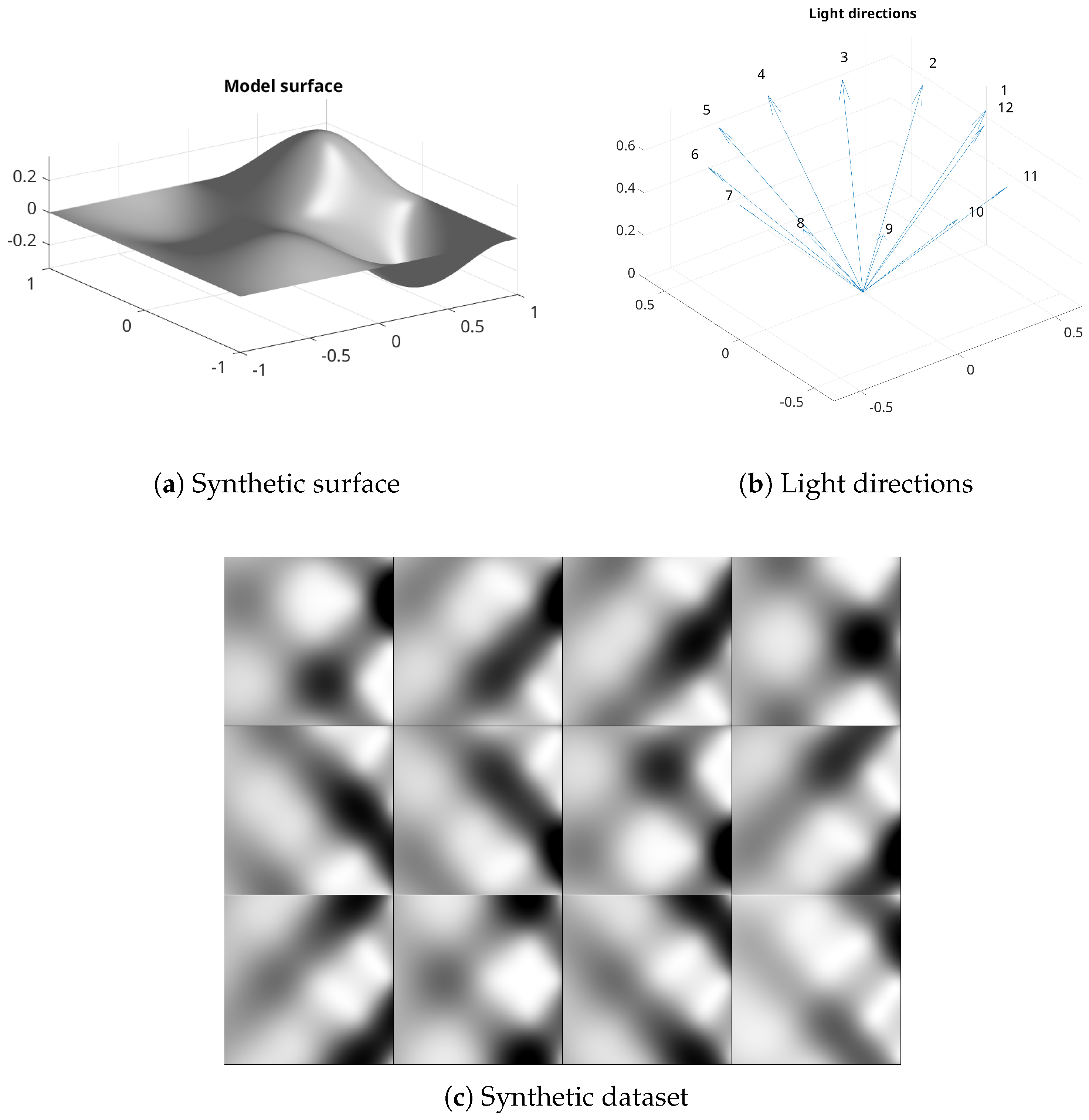
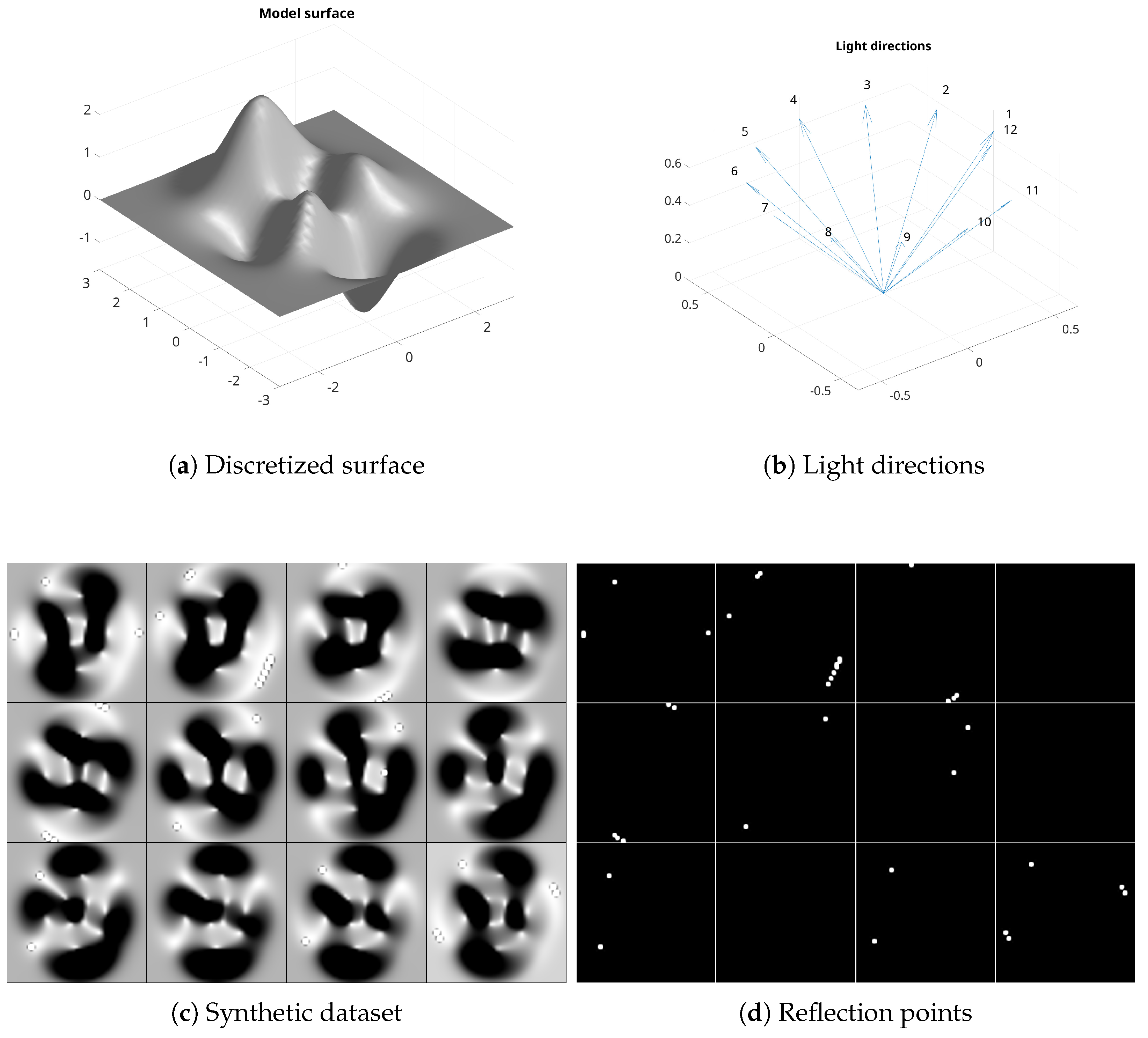
Figure 3 displays a synthetic dataset generated by the package, corresponding to a surface available in the choosefun function; see Figure 3a. The lighting directions, plotted in Figure 3b, are obtained by considering 12 angles between 0 and $11\pi /6$. Here, we consider a constant albedo and set $A=2$, $r=s=101$, obtaining the dataset displayed in Figure 3c.

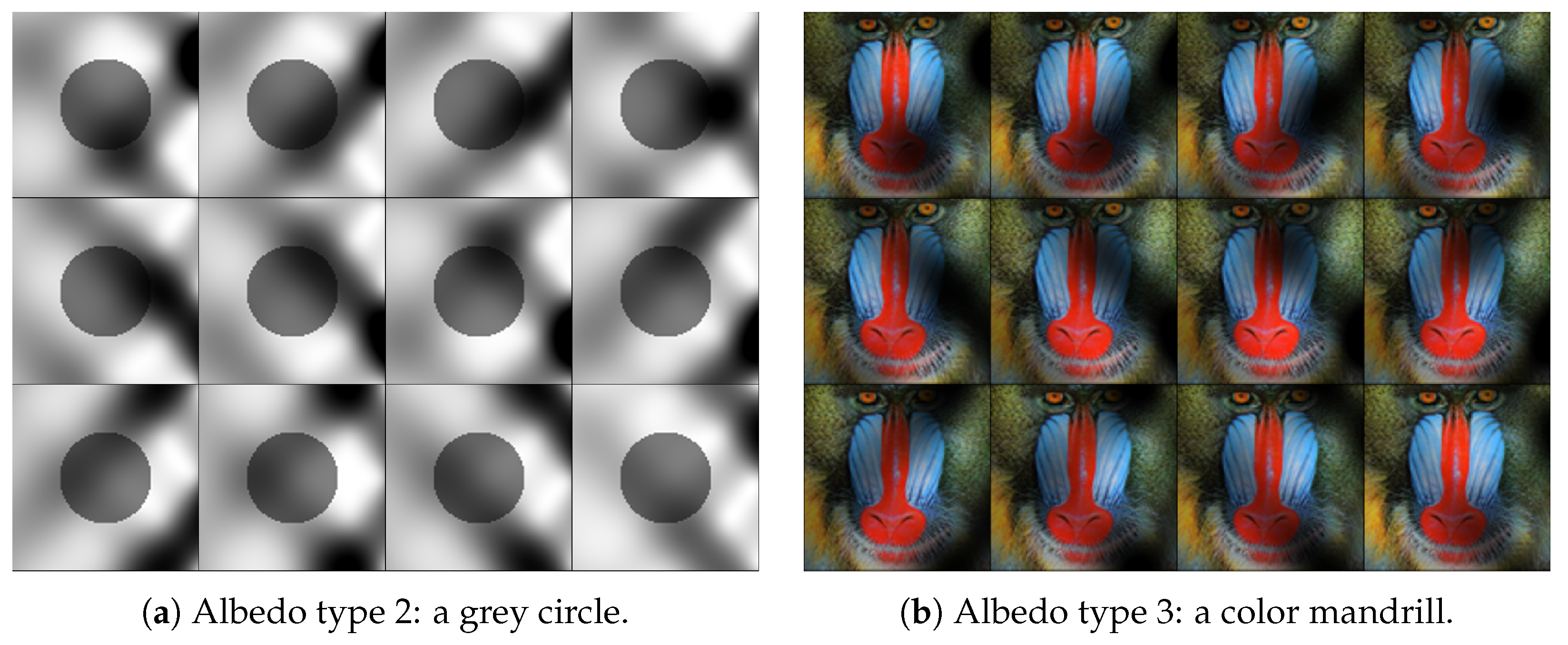
The presence of a color RGB albedo causes the final data matrix M to have dimensions $p\times q\times 3$. The three layers of the matrix contain RGB information for each data image. In the computation, the matrices containing normals and lights vectors are the same, only the albedo matrix changes according to red, green, and blue color channels. Figure 4 shows two datasets, corresponding to the same surface and light positions as in Figure 3, with two different albedos, both generated by the function makealbedo.

If the input parameter reflectau is zero, the surface is assumed to be a perfect Lambertian reflector. If it is nonzero, it must be a vector containing the constants ${\tau }_R$ and ${\kappa }_R$ of Equation (7), and the construction described in Section 4 is employed. Figure 5 shows an example of a discretized reflecting surface. The lighting directions are the same used in Figure 3, the albedo is constant. Setting ${\tau }_R=0.1$ and ${\kappa }_R=5$, we obtain the dataset displayed in Figure 5c, which presents reflection points. Such points are visualized in Figure 5d, reporting the difference between the reflective dataset and a nonreflective one.

The entries of the parameter intens, if provided, are used as 2-norms of the columns of L, that is, as lights intensity. If autoexp is set to 1, each image in the dataset M is divided by the largest pixel value in that image, ensuring that the brightness reaches its maximum. The parameter atten selects the attenuation factor ${\delta }_{i,j}$ for close lights: if its value is 1, ${\delta }_{i,j}={\parallel {\mathsf{\ell }}_i-{\mathbf{v}}_j\parallel }^{-2}$, if it is 0, then ${\delta }_{i,j}={\parallel {\mathsf{\ell }}_i-{\mathbf{v}}_j\parallel }^{-1}$; see the discussion in Section 3 and Section 9.7 from [30].

5.5. psdatagen

The scripts psdatagen provides a practical example of the construction of a dataset. We give an algorithmic description of the process.

• The script initially sets some constants that characterize the type of PS scenario, and some visualization parameters. Such constants have easily comprehensible names and are extensively commented in the code. Their names resemble, as much as possible, the notation introduced in previous sections.
• The first step consists of constructing the model surface. As already noted, the software accepts two formats for the surface of the target: its analytical expression or a discretization. Such alternatives are implemented in the code by a struct variable, called surface. In the first case, it contains the functions u, $u_x$, and $u_y$ returned by choosefun, in the second one, three matrices X, Y, and Z, containing the coordinates of each point of the discretization.
• The variable ray is then introduced for the purpose of selecting the distance of the light sources from the target. If its value is zero, the standard setting with lights at infinite distance is selected. A non-zero value represents the distance between the light sources and the reference origin. Similarly, the reflectau parameter is set to activate or deactivate surface reflection, as discussed in the notes to the makepsimages function.
• Then, the position of the light sources is set. Various choices for the angles around the z axis are contained in the script, and the vector $\mathbf{z}$ contains the z coordinate of each source. At this point, the light matrix L is constructed by calling the createlights function. The matrix can be optionally perturbed by Gaussian noise.
• If the variable ray is nonzero, homogeneous coordinates for each source are stored in the column of the matrix $L_h$. This notation signals to the function makepsimages that a scenario with “close” lights has been selected.
• Finally, the albedo is obtained by the makealbedo function, and the dataset is constructed by a call to makepsimages.
• Results are plotted in different figures: the model surface, light directions, and the dataset. If reflection is activated, a further figure displays the difference between images with and without reflection.

The variable produced by psdatagen are the following:

• M: PS data matrix;
• $N,L,D$: normal vectors, light positions, and albedo;
• $X,Y,Z$: discrete coordinates of the synthetic object points;
• $r,s$: image size;
• $A,B,h$: physical size of the observed scene and pixels size.

The computed data can be used as a test dataset for any method intended to solve the photometric stereo problem. In particular, given the possibility to set the parameters at will, the user can create datasets of any size, under very different observation conditions, to be used as training data for machine learning methods. Furthermore, since the algorithms are coded through high-level vector and matrix operations, their Matlab implementation is quite efficient and is automatically parallelized in a multi-core or multi-processor environment, making the software considerably fast.

To illustrate this aspect, the script genbigdataset has been included in the package. It allows to select:

• a list of model functions $f_1,\dots ,f_{n_1}$;
• a list of reflection tolerances ${\tau }_1,\dots ,{\tau }_{n_2}$;
• a list of noise levels ${\sigma }_1,\dots ,{\sigma }_{n_3}$;
• the number of light sources $n_L$.

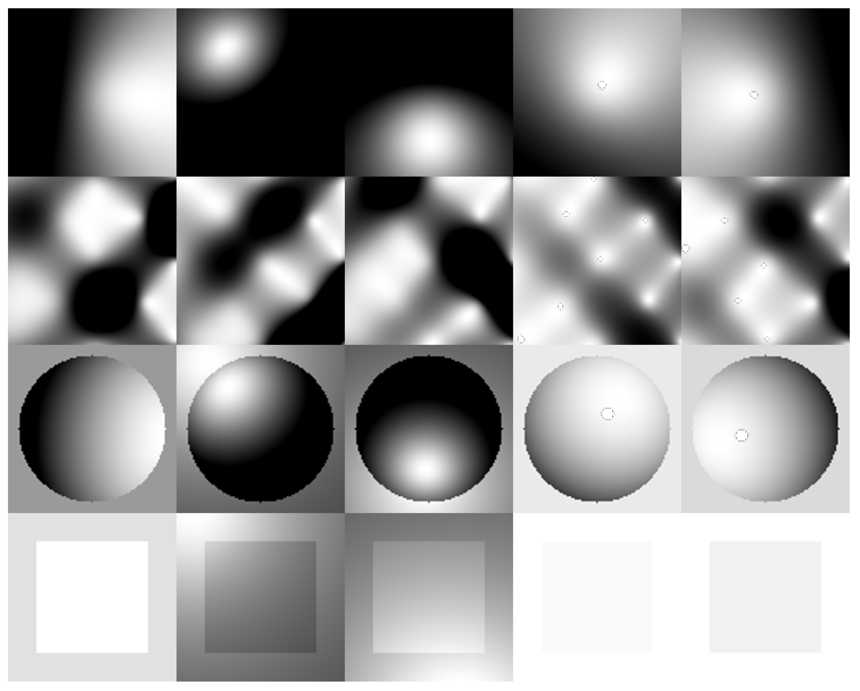
The script constructs $n_L$ random light directions (sources at infinite distances) and $n_L$ light positions at a finite distance. Then, it constructs synthetic pictures corresponding to all possible combinations of such parameters, generating $2n_1{n}_2{n}_3{n}_L$ test images.

As an experiment, we fix $n_1=5$, $n_2=n_3=2$, and $n_L=100$ (see the code of the function genbigdataset.m) to generate 4000 images at resolution $101\times 101$. The scripts runs in less than 4 seconds on a desktop computer. Figure 6 shows 20 images extracted from the resulting dataset.

6. Some Numerical Simulations

To investigate the quality of the datasets produced by the package proposed in this paper, we present here some numerical experiments.

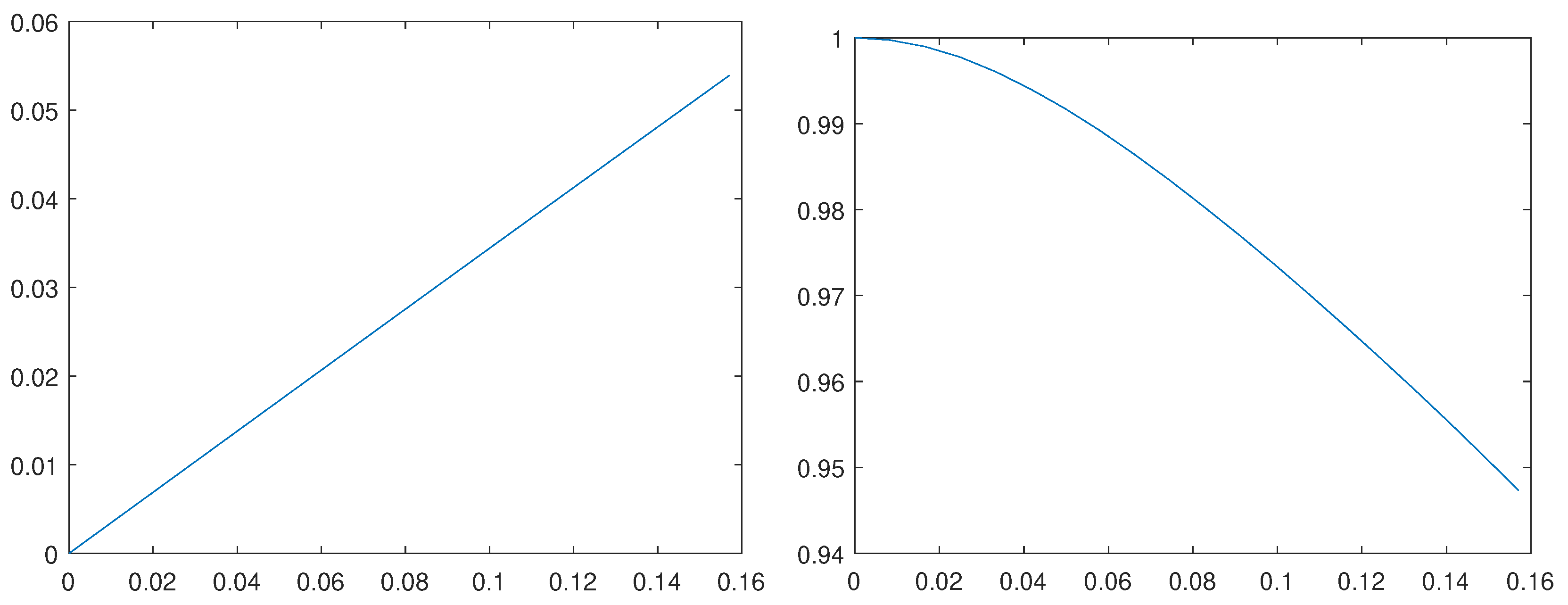
We start with a sensitivity analysis. A picture is generated by illuminating a model surface from a direction identified by a chosen vector. Then, the vector is progressively rotated around the z axis up to the angle $\pi /20$ radiants. For each rotation step, a new picture is generated and compared to the initial one.

Figure 7 shows the root mean squared error (RMSE) and the structural similarity (SSIM) for each image of the sequence, as computed by Matlab functions rmse and ssim, versus the angle measured in radiants. It can be seen that the RMSE linearly converges to zero as the angle decreases.

The results of a similar sensitivity analysis for the lighting distance are displayed in Figure 8. In this case a light source is initially placed at distance A (the horizontal size of the observed scene) from the target. Then, the light is progressively moved away from the subject, up to the distance $40A$. Each picture is compared to the image corresponding to a source at infinite distance. In this case, the RMSE converges to zero exponentially as the distance increases.  

We now test the performance of a dataset produced by our package as input for a reconstruction algorithm. We consider the model surface of Figure 3 and construct a sequence of datasets, each one of 7 images of size $401\times 401$. Each dataset is produced with light sources at fixed directions and distance $\gamma A$ from the observed target, with 

$$\gamma \in \{1,3,10,30,100,300,1000,\infty \},$$

where $\gamma =\infty$ means that the lights are positioned at infinite distance from the surface.

Each dataset is used as input for the reconstruction algorithm coded in the package ps3d from [26], available at https://bugs.unica.it/cana/software.html (accessed on 27 April 2025). Such algorithm first computes the normal vectors as columns of the matrix $\tilde{N}$, approximating N in (3), and then reconstructs the surface by a finite difference approach applied to a Poisson differential problem, as outlined in Section 2. This method assumes that the surface is Lambertian and that the light sources are at infinity, so we expect small errors when $\gamma =\infty$ and increasing errors as $\gamma$ takes smaller values.

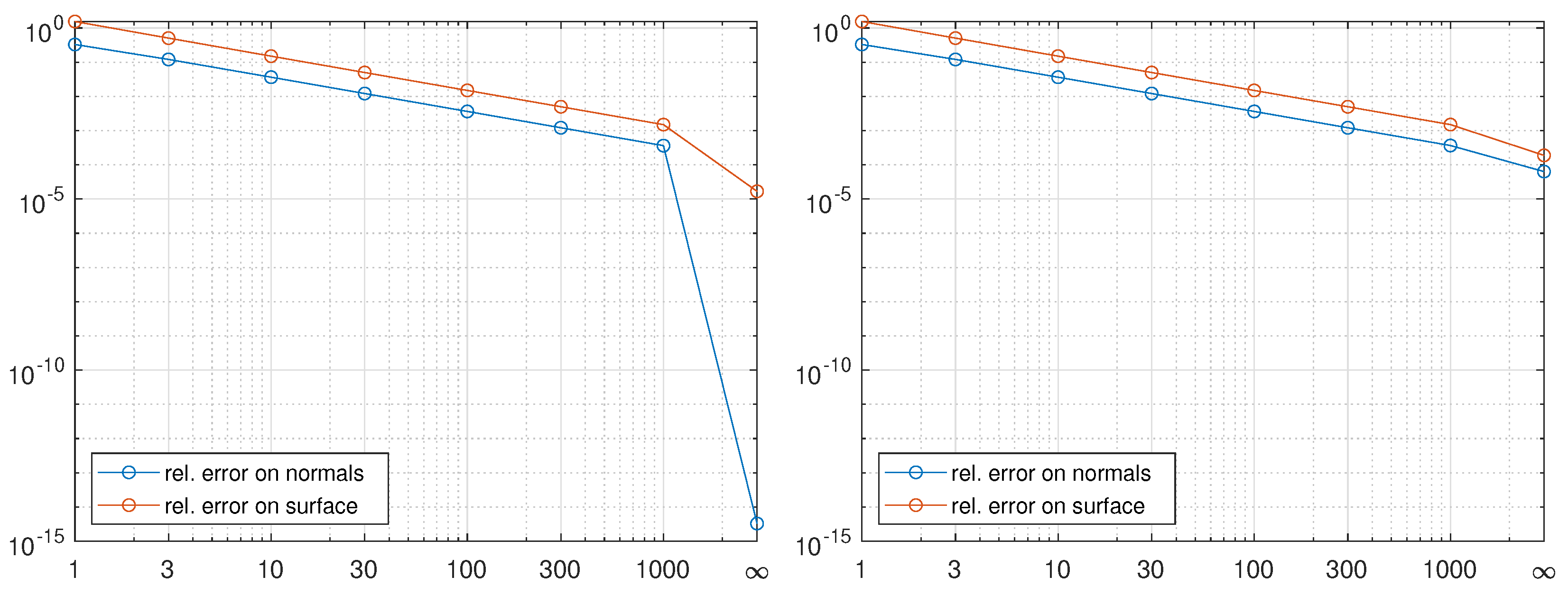
To evaluate the quality of the reconstruction we consider the relative errors on the normal vectors and the surface

$${\displaystyle \frac{\parallel N - \tilde{N}{\parallel }_F}{{\parallel N\parallel }_F}},{\displaystyle \frac{\parallel U - \tilde{U}{\parallel }_F}{{\parallel U\parallel }_F}},$$

where U contains the values of the model function on the grid, $\tilde{U}$ its numerical approximation, and ${\parallel ·\parallel }_F$ denotes the Frobenius norm.

Such relative errors are displayed in the left graph of Figure 9. We can see that when $\gamma =\infty$ the normal vectors are approximated at machine precision, showing that the synthetic dataset produced by the package is perfectly compliant with the assumptions of the standard PS model. The reconstruction error for the surface is about ${10}^{-5}$, in line with the central differences approximation used to solve the Poisson problem, which ensures an error or order $O\left(h^2\right)$, where $h\simeq 5·{10}^{-3}$ in this particular setting.

When the light sources get closer to the observed surface, the errors increase. Indeed, the dataset become “non ideal”, as it progressively violates more and more the assumptions of the standard model.

We show here how a synthetic dataset may be used to simulate particular experimental conditions. When pictures are taken with a camera set for automatic exposure, the light conditions are automatically optimized for each picture. The default option for the function makepsimages is to use a “fixed” exposure for all images, but a simulation of automatic exposure can be activated by setting the input variable autoexp to the value 1, as discussed in Section 5.

The graph on the right of Figure 9 reports the results obtained by repeating the previous experiment with “automatic exposure”. Most of the errors slightly increase, showing that it is preferable to disable automatic exposure in the camera before collecting images. In particular, we observe a strong worsening of both the normal vector computation and the surface reconstruction when light sources are at infinity, situation that is practically encountered when sunlight can be used for illuminating the observed scene.

7. Conclusions

This paper presents an open source software tool to construct datasets for shape from shading problems under specific conditions. In addition to the standard photometric stereo ideal setting, light sources can be placed at any distance from the target, and surfaces with specular reflection can be simulated by the software. The chosen object surface is represented either by explicit formulae or by a discretization, and the albedo can be a grayscale or a color image. Large datasets can be constructed reproducing several observation conditions by simply setting some parameters, allowing to construct large datasets for training neural networks. Differently from available datasets, which only reproduce fixed configurations, one can freely recreate any specific condition. This allows to employ the package in different fields, e.g., in archaeology, where is extremely useful to be able to simulate particular scenarios. Having the exact solution at disposal is essential to estimate the accuracy of new algorithms, allowing to understand the reason for failures, test which algorithmic changes lead to an improvement in accuracy, and experiment with particular shooting techniques.