From Transformers to Voting Ensembles for Interpretable Sentiment Classification: A Comprehensive Comparison

Abstract

This study conducts an in-depth investigation of the performance of six transformer models using 12 different datasets—10 with three classes and two with two classes—on sentiment classification. We use these six models and generate all combinations of triple schema ensembles, Majority and Soft vote. In total, we compare 46 classifiers on each dataset and see in one case up to a 7.6% increase in accuracy on a dataset with three classes from an ensemble scheme and, in a second case, up to 8.5% increase in accuracy on a dataset with two classes. Our study contributes to the field of natural language processing by exploring the reasons for the predominance, in this particular task, of Majority vote over Soft vote. The conclusions are drawn after a thorough investigation of the classifiers that are co-compared with each other through reliability charts, analyses of the confidence the models have in their predictions and their metrics, concluding with statistical analyses using the Friedman test and the Nemenyi post-hoc test with useful conclusions.

1. Introduction

The amount of data generated daily on the internet is enormous. If we manage these data effectively, their value multiplies. High-quality data can lead to valuable conclusions, and combined with critical thinking and knowledge, can be used for predictions or even diagnoses. However, within this massive production of data, there is also ‘noise’, i.e., information that is irrelevant or unhelpful, which increases computational costs without adding much value [1,2]. It is therefore critical to filter out the noise before proceeding to model training. One of the most challenging areas of natural language processing is the detection and categorization of emotion through text. Understanding sentiment is important for improving services based on data analytics, such as financial services, but also for creating better predictive models. The goal of the scientific community is for models to understand natural language in depth, with emotion playing a key role in the whole process. Categorizing emotions is often difficult, even for humans, let alone machines. The difficulty increases when the data contains ironic or ambiguous emotions, or when the datasets include multiple classes, such as “negative”, “neutral” and “positive”. The neutral class can be most confusing as often it borders the other two, making it difficult to decide; besides, classes can partially overlap each other, which means similar texts will be classified under different categories. Proper preparation of the training data is imperative [3]. A sufficient amount of data is required and, in this paper, we will analyze this further. Clear categorization and training of models for several epochs is required to be able to learn the patterns present in the given set. At the same time, the models used must be suitably designed to process these data, balancing accuracy with computational requirements. In recent years, transformer models have dominated the field of natural language processing, bringing excellent results. Many different models have been developed, some of which focus on saving computational resources, while others prioritize accuracy or offer a compromise between the two. We focused on medium-sized transformers, so that the experiments can be implemented on not very expensive hardware. In any case, the experimental procedure and ultimately the conclusions drawn are independent of the models, because we are dealing with processes and characteristics that any classifiers can have.

The reminder of the article is structured as follows. Section 2 presents related work. Section 3 presents the methods and the experimental procedure. Section 4 presents the experimental results and the main findings. Finally, Section 5 concludes the article and draws directions for future work.

2. Related Work

The related works are generally about model comparison and method finding. The first study considered here investigates the effectiveness of transfer learning models, such as BERT, RoBERTa, Albert, DistilBERT and XLNet, in sentiment classification and specifically binary categorization. Although attention-based models, such as BERT and XLNet, have proven to be particularly powerful in natural language understanding, they face difficulties in specific domains, such as the language of social networking platforms. The results, after fine-tuning with the same hyperparameters, showed an Accuracy of 98.30 for RoBERTa, 98.20 for XLNet, 97.40 for BERT, 97.20 for Albert, and 96.00 for DistilBERT [4].

The second study we considered investigates the performance of self-supervised transformer-based models for multi-class sentiment analysis on a non-standard dataset. Although the models discussed herein, namely BERT, RoBERTa, and Albert, have different designs, they share a common objective: to leverage large-scale text data in developing a general-purpose language understanding system. The performance of these models, once fine-tuned with the proposed architecture, is evaluated based on the F1-score and AUC (Area Under the ROC Curve). Among these models, BERT had the best F1-score of 0.85, followed by RoBERTa with an F1-score of 0.80 and Albert with an F1-score of 0.78. This proves that the proposed architecture with the BERT model is the best choice for multi-class sentiment analysis on non-standard datasets [5].

The next study we considered examines sentiment analysis in Greek consumer reviews, filling a gap in the literature, as existing research focuses mainly on social media posts and uses traditional machine learning (ML) methods. The aim of the research was to compare the performance of modern methods, such as artificial neural networks (ANNs), transfer learning (TL) and large language models (LLMs), against traditional ML models on a dataset of Greek product reviews. The results showed that the GreekBERT and GPT-4 models outperform significantly, with GreekBERT achieving 96% Accuracy and GPT-4 95%, while ANNs had a performance similar to ML models. The study confirms the hypothesis that modern methods, especially BERT, excel in sentiment classification on Greek data [6].

In another study, the performances of deep learning and traditional machine learning techniques in sentiment analysis in customer reviews were compared. The deep learning models employed are Convolutional Neural Network and Recursive Neural Network, whereas traditional ones include Logistic Regression, Random Forest, and Naive Bayes. They employed Amazon product review data, for which the star rating served as an indicator of each review’s sentiment. Through multiple experiments, model performance was considered with respect to both accuracy and efficiency of sentiment detection. Five models were compared for classification: three traditional machine learning algorithms, including Logistic Regression, Naive Bayes, and Random Forest, and two deep learning models, RNN and CNN, to see their effectiveness in sentiment analysis from customer reviews. The results showed that Random Forest and Logistic Regression achieved the highest Accuracy at 0.99, followed closely by RNN with 0.98 and CNN with 0.93, while the lowest given was by Naive Bayes with an Accuracy of 0.84 [7].

The next study examines the public’s sentiments on education reform issues by utilizing a state-of-the-art deep learning AraBERT language model. The authors developed a dataset comprising 216,858 tweets related to the reform topic and manually annotated 2000 of those tweets with their respective sentiments. They present several models compared with fine-tuned AraBERT: CAMeLBERT, MARBERT, GPT, baseline Random Forests, SVM, and Logistic Regression. AraBERT attained an F1-score of 0.89, which outperforms the baseline models by 5% and other transformer-based models by 4%, hence showing the importance of language and domain-specific models in Arabic sentiment analysis [8].

Another study analyzed Amazon reviews that span different product categories to classify their sentiments using different techniques: natural language processing, machine learning, ensemble learning, and deep learning. This is achieved through processes that include data collection, preprocessing (normalization and tokenization), and feature extraction using methods such as Bag-of-Words and TF-IDF. Among others, some of the popular machine learning algorithms that have been tried in this domain include Multinomial Naive Bayes, Random Forest, Decision Tree, and Logistic Regression, whereas the ensemble learning method tried is Bagging. Simultaneously, there are deep learning algorithms such as CNNs, Bidirectional LSTMs, transformer-based XLNet, and BERT. According to different evaluation metrics like Accuracy, Precision, Recall, F1-score, etc., the most efficient performance was given by BERT: it achieved a high Accuracy value of 89% [9].

In another study, the authors focused on misinformation detection. They proposed a misinformation detection method that merges multimodal features using transformers and evaluates credibility with self-attention-based Bi-RNN networks. First, semantic descriptions of images were obtained by generating captions from them using an image captioning model. These captions were then compared with the surrounding text by fine-tuning transformers to check for semantic consistency. Further, another transformer was fine-tuned on the text independently for sentiment classification to bring the sentiment features into the text representation by merging the output. Then, a credibility assessment model was trained on Multi-Cell Bi-GRUs with self-attention to identify misinformation. The experimental results of the analysis show that the best performance, with an Accuracy of 0.904 and an F1-score of 0.921, was achieved by performing feature fusion using augmented embeddings from sentiment classification results [2].

In another study, virtual simulators of embedded systems are presented and student surveys on their use in the initial stage of the embedded systems learning process are analyzed. The questionnaires were written in Polish and the answers were automatically translated into English using two publicly available translators. The results of users’ experiences and emotions related to the use of virtual simulators were presented based on the identified emotion using three selected analysis methods: the NLP Flair library, the Pattern library and the NLP BERT model. The results of the selected sentiment detection methods were compared and correlated with the users’ report responses, which provides information about the quality of the methods and their potential use in the automated review analysis process. This paper includes detailed sentiment analysis results with a broader statistical approach for each question. Based on student feedback and sentiment analysis, a new version of the TMSLAB v.2 virtual simulator was created [10].

Another study combines the advantages of voting and boosting methods and proposes a novel two-stage simultaneous learning set voting-boosting (2SVB) method for social network sentiment classification. This new method not only establishes a concurrent set framework to reduce computation time, but also optimizes the use of erroneous data and improves the performance of the set. To optimize the utilization of erroneous data, a two-stage training approach was applied. Stage 1 training was performed on the datasets using a three-fold cross-segmentation approach. Stage 2 of training was performed on datasets enriched with the erroneous data predicted by stage 1. To increase the diversity of the base classifiers, the training stage used five pre-trained deep learning (PDL) models with heterogeneous pre-training frameworks as base classifiers. To reduce the computation time, a two-stage simultaneous ensemble framework was created. Experimental results demonstrated that the proposed method achieved an F1-score of 0.8942 on the coronal tweet sentiment dataset, outperforming other comparable ensemble methods [11].

The last work we considered is a sentiment classification strategy applied based on the Majority Vote principle of multiple classification methods including Naive Bayes, SVM, Bayesian Network, C4.5 Decision Tree and Random Forest algorithms. In this experiment, six individual classification approaches and the proposed ensemble approach were all trained and tested using the same dataset of 12,864 tweets, in which 10-fold evaluation was used to validate the classifiers. The results show that the proposed ensemble approach outperforms these individual classifiers on this Twitter airline dataset. Based on those authors’ observations, the ensemble approach could improve the overall accuracy in Twitter sentiment classification for other services as well. The ensemble classifier also achieved the highest Accuracy, which is 91.7% [12].

3. Methods and Experimental Procedures

In this section, we will describe in detail the steps of the experimental procedure that we followed and in general the purpose of this work.

First, we proceed to present the datasets we used in this research and their preprocessing; we continue with the pre-trained models of the six transformers, what their architecture is and how different they are. We highlight the metrics we selected and then present the framework of the experimental procedure that illustrates the workflow of the serial-structured classifier comparison process and the derivation of a proposed ensemble method for each set and final winner (proposed method—final ensemble scheme) for all these 12 datasets.

In this research, we have utilized datasets and pre-trained transformer models from the Hugging Face community, as well as open-source material [13].

3.1. Datasets and Preprocessing

The datasets selected for the current study were 12, focusing exclusively on sentiment analysis. These have been taken from different sources and pertain to various subjects like climate, finance, airlines, social networks, and so on. The characteristics of each dataset are presented in

Table 1. The 12 datasets used in the paper and their characteristics.

#	Dataset	Abbreviation	Classes	Size	Class Distribution	Description
1	climatebert/climate_sentiment	climate_3cl	3	1320	Positive: 571, Neutral: 448, Negative: 301	Tweets and texts on climate change
2	cardiffnlp/tweet_eval (sentiment)	cardiffnlp_3cl	3	59,899	Positive: 27,479, Neutral: 21,043, Negative: 11,377	Tweets with general emotional content
3	Sp1786/multiclass-sentiment-analysis-dataset	Sp1786_3cl	3	41,643	Positive: 14,022, Neutral: 12,208, Negative: 11,079	Includes texts on a variety of topics with sentiment analysis
4	sudhanshusinghaiml/airlines-sentiment-analysis	US_Airlines_3cl	3	14,640	Positive: 2363, Neutral: 3099, Negative: 9178	Analyses customer satisfaction of airlines through feedback
5	zeroshot_twitter-financial-news-sentiment	0shot_twitter_3cl	3	11,931	Positive: 7744, Neutral: 2398, Negative: 1789	Tweets about financial markets
6	indonlp/NusaX-senti (eng)	NusaX_3cl	3	1000	Positive: 239, Neutral: 383, Negative: 378	Comments translated into English
7	takala/financial_phrasebank	takala_50_3cl takala_66_3cl takala_75_3cl takala_100_3cl	3	4846 4217 3453 2264	Positive: 1363/1168/887/570 Neutral: 2879/2535/2146/1391 Negative: 604/514/420/303	Financial news with different commentator agreement rates
8	cardiffnlp/tweet_eval (irony)	cardiffnlp_2cl	2	4601	Non-ironic: 2389, Ironic: 2212	Tweets with or without irony
9	carblacac/twitter-sentiment-analysis	carblacac_2cl	2	181,986	Positive: 91,048, Negative: 90,938	Large dataset for sentiment analysis in tweets

.

As described above, the selected datasets contained only texts with sentiment tags. We kept only the columns that contained text and the corresponding sentiment label, and removed all other columns that the dataset might have had. We then cleaned the data using various text preprocessing techniques, without proceeding to any artificial augmentation of the data or any class balancing. These techniques are widely used in Natural Language Processing (NLP) and aim to improve the quality of the data before applying machine learning models, specifically transformers.

First, we removed all words that do not provide important information, such as articles and links. We also excluded those elements that have no semantic or emotional value, such as URLs, HTML tags, and usernames like @username. We also excluded emojis, which could be the subject of another study regarding their effect on model performance. This study, however, will deal exclusively with plain text.

Preprocessing continued with the removal of punctuation marks, which add noise to the analysis; extended contractions, such as “don’t”, were converted to “do not” for easier processing. We split alphanumeric strings into different words or numbers, normalized elongated characters, for example, “loooove” was converted to “love”, and removed all non-alphabetic characters. Then, throughout the text we converted uppercase letters to lowercase, achieving a reduction in vocabulary complexity, and noise reduction during model training. Finally, we checked and deleted the blank instances if there were any.

All these preprocessing steps were performed on all 12 datasets used for this research study.

We can combine all these datasets—10 sets with three classes and two sets with two classes—into two bigger sets and perform the algorithm comparisons there. However, that approach would deprive us of the detailed analysis of model behavior under various conditions.

In particular, we want to examine how the models perform on both small and large datasets, as well as on balanced or unbalanced sets in terms of their classes. Rather than limiting ourselves to comparing the models on two single sets, we aim to investigate their performance on a wider range of data in order to better understand their performance and generalization in different scenarios.

3.2. Pre-Trained Transformer Models

In this paper, we selected six different pre-trained transformer models to compare them on the datasets described above. Training a model from scratch requires huge amounts of data and significant computational resources (GPU/TPU), which makes the use of pre-trained models highly efficient. These models have already learned general language structures, syntactic and semantic patterns, which allows their optimization (fine-tuning) with a smaller amount of data. This improves both performance and adaptation to the task at hand, such as sentiment analysis, by leveraging the principle of transfer learning [14].

We selected models with different architectures and design approaches, while maintaining a micro-medium size, so that they can be trained on affordable computing infrastructures. Also, the incorporation of smaller models in the experimental process involves the following exploratory control: Could it be that by incorporating models that are indeed smaller and individually do not perform very well, we could lead to a scheme that exhibits improved performance because these individual models exhibit diversity? In other words, we are investigating whether an older and smaller version of GTP, e.g., GTP2, is a more efficient choice in the context of an ensemble than a larger and newer version such as GPT-NeoX (Pythia). Why would this be the case with GTP2? In

Table 2. Models and abbreviations.

Transformers	Abbreviation
facebook/bart-base [15]	Bart
MoritzLaurer/DeBERTa-v3-base-mnli-fever-anli [16,17]	DeBERTa
openai-community/gpt2 [18]	GPT2
EleutherAI/pythia-410m [19,20]	Pythia
google-t5/t5-base [21]	T5
albert/albert-base-v2 [22]	Albert

, we present the names of the models and the abbreviations we will use in the following.

This is followed by an introduction to the research models through comparisons between them, highlighting their strengths and limitations.

Table 3. Summary comparison.

Transformers	Architecture	Specialty	Training Direction
Bart	Seq2seq	Text Generation, Text Classification	Bidirectional
DeBERTa	Bidirectional Transformer	Natural Language Inference, Text Classification	Bidirectional
GPT2	Autoregressive Transformer	Text Generation, Language Modeling	Unidirectional
Pythia	Autoregressive Transformer	Text Generation, Language Understanding	Unidirectional
T5	Seq2Seq	Text-to-Text Tasks (e.g., Translation, Summarization)	Bidirectional
Albert	Optimized BERT	NLU, Text Classification	Bidirectional

provides a summary comparison of the models, highlighting their diversity.

Arguments for the Diversity of the Six Models and the Risk of Over-Simplification

One could easily be led to wrong conclusions by comparing these models only on the basis of this table. However, when it comes to pre-trained transformer models, it would be wrong to rush to simplistic conclusions, for the differences among them do not only reside in parameter magnification or different trainings but implicate critical design decisions with repercussions on their capacity to understand language, adapt to new data, and perform computations efficiently.

• Different model architectures affect model performance:
  • The Bart (or BART) model [15] is a sequence-to-sequence transformer that encompasses the best elements of BERT, with bidirectional encoding, and GPT, with autoregressive decoding. This makes it very powerful for text generation and denoising tasks but less efficient in pure sentiment classification without fine-tuning.
  • DEBERTA [16] utilizes disentangled attention και relative position embeddings into attention process, enhancing its understanding of word relationships. However, it does retain absolute position embeddings before the softmax layer to keep the idea of the absolute position of words for the prediction.
  • GPT2 [18] uses causal language modeling with masked self-attention [23], providing the possibility to predict each word based on previous words. This approach makes it perfect for coherent text, but in terms of sentiment analysis without fine-tuning, its results will be limited, as opposed to bidirectional models like BERT, due to the fact that this does not take into account the whole context at once.
  • The Pythia model [19] is based on GPT-NeoX, an evolution of the transformer architecture. GPT-NeoX introduces techniques such as Rotary Positional Embeddings (RoPE), which improve the model’s ability to handle larger data sequences. It is one of the latest major language models, open source, adapted for generalized text understanding.
  • The T5 model [21] is a sequence-to-sequence transformer which manages all tasks in a text-to-text framework, allowing it to act as a more general classification framework.
  • The Albert model [22] optimizes BERT by reducing parameters via a parameter sharing factor, which makes it more efficient on smaller GPU infrastructures.

All the above models, with appropriate fine-tuning on sentiment classification datasets, can achieve high performance. It is obvious that a brief comparison of the transformer models is not sufficient as their differences are not limited to size or general performance, but are influenced by their architecture (bidirectional, autoregressive, text-to-text), training method (Masked Language Modeling vs. Causal Language Modeling) [18,24], efficiency on different datasets and tasks, and their computational complexity and practical utility. Therefore, any comparison should take into account multiple metrics and parameters and not just summary scores.

Furthermore, the models we used in the paper are pre-trained, so it is important to mention that pre-training and fine-tuning are two critical phases in the development of natural language processing (NLP) models. Pre-training involves training a model on large and diverse datasets, such as BookCorpus and Wikipedia, to learn general language representations. This process allows the model to understand basic language properties, such as syntax, semantics and context, without having to start from scratch for each new task.

After pre-training, the model undergoes fine-tuning, where it is adapted to specific datasets for specialized tasks. For example, datasets such as GLUE, SQuAD and CNN/DailyMail are used for tasks such as text classification, question answering and text generation. Fine-tuning allows the model to focus on specific information and optimize its performance for the specific task, so this point is also critical to the overall behavior of a pre-trained model [14].

After several tests of the models in fine-tuning with grid search, we selected the best hyperparameters. Transformer models are probabilistic and not deterministic which means that even for the same data with the same parameters, each individual run or training will give us slightly different metrics. There are various causes that contribute to these small deviations. These are the randomness of the initialization of the weights, the order of the data during training, and the use of techniques such as dropout.

3.3. Metrics

To ensure a thorough evaluation of the classifiers in this paper, six key metrics are used to measure the performance of the models. Metrics such as Accuracy, F1-score, Precision, Recall, Matthews Correlation Coefficient (MCC) and Cohen’s Kappa are described below, with their respective mathematical formulas. Specifically, for the winning transformer models, in addition to these metrics we will also examine the Mean Confidence for correct and incorrect predictions and the Expected Calibration Error (ECE), while in the Results section we will analyze the confusion tables, reliability charts and SHAP summary charts, essentially explaining the reasons for their performance and what challenges they may have faced.

3.3.1. Accuracy

Accuracy is likely the easiest and most typical performance measure for testing the performance of a classifier. Accuracy measures the number of correct predictions out of all examples, i.e., how often the model predicts the positive or the negative class correctly [25]. Accuracy can be calculated as follows:

Accuracy = (TP + TN)/(TP + TN + FP + FN)

(1)

• TP (True Positives): True Positive predictions
• TN (True Negatives): True Negative predictions
• FP (False Positives): False positive predictions
• FN (False Negatives): False Negative predictions

Accuracy is useful when data are balanced, i.e., the classes contain approximately the same number of samples. In class imbalance situations, however, Precision can give false good outcomes and needs to be combined with other performance metrics.

3.3.2. Precision

Precision is a measure of performance that estimates the ratio of accurately classified positive predictions out of a classification model. Is the number of True Positives divided by all the cases predicted positive [26]. It answers the question: “Out of all the cases the model labeled as positive, how many were actually positive?” Precision can be computed by the following equation:

Precision = TP/(TP + FP)

(2)

High Precision implies that a low number of false positives are generated, which is very useful for scenarios where false alarms are costly or harmful, such as medical diagnosis or fraud detection. Precision does not consider the false negatives, however, so it is usually used in combination with Recall for a more complete assessment.

3.3.3. Recall

Recall, synonymously referred to as sensitivity or true positive rate, is a metric that determines the extent to which a model correctly predicts all cases of the positive class. It is a measure of the proportion of true positive cases that were predicted to be positive by the model. [25]. Recall fundamentally answers the question: “Out of all the true positive cases, how many did the model correctly detect?” The formula for Recall is the following:

Recall = TP/(TP + FN)

(3)

High Recall is required in applications where missing a positive case would be disastrous, e.g., disease diagnosis or fraud detection. However, putting weight on Recall alone will result in high false positives, so it is usually combined with Accuracy for a more balanced evaluation.

3.3.4. F1-Score

The F1-score is a very important metric that combines both Precision and Recall into a single score, providing a balanced view of a model’s performance. It is the harmonic mean of Recall and Precision, assigning equal importance to both metrics. The F1-score is particularly useful in the situation of imbalanced data, where one class is considerably more frequent than the other [27]. The formula for the F1-score is as follows:

F1 = 2 ∗ (Precision ∗ Recall)/(Precision + Recall)

(4)

This metric is useful in cases where it is important to strike a balance between not getting false positives and not getting false negatives. A high F1-score indicates the model has high Precision and high Recall, i.e., it accurately classifies positive cases and does not make many wrong predictions. Because it does not take true negatives into consideration, it is best utilized in cases where the positive class is of more concern or higher risk.

3.3.5. Matthews Correlation Coefficient (MCC)

MCC is a correlation coefficient used to measure the quality of binary classifications. It is particularly useful when classes are unequally distributed.

$$\mathrm{MCC}={\displaystyle \frac{\left(\left(\mathrm{TP}\ast \mathrm{TN}\right)–\left(\mathrm{FP}\ast \mathrm{FN}\right)\right)}{\sqrt{\left(\mathrm{TP}+\mathrm{FP}\right)\ast \left(\mathrm{TP}+\mathrm{FN}\right)\ast \left(\mathrm{TN}+\mathrm{FP}\right)\ast \left(\mathrm{TN}+\mathrm{FN}\right)}}}$$

(5)

A high MCC indicates that the model has a good ability to discriminate between classes, even when classes are unevenly distributed. This is important in sentiment analysis, where classes may not be balanced. The MCC score ranges from −1 (completely wrong predictions) to 1 (perfect predictions), and 0 means that the model is no better than a random choice [28].

3.3.6. Cohen’s Kappa (κ)

Cohen’s Kappa measures the agreement between two classifications, taking into account the probability of random agreement. The formula for κ (Kappa) is as follows:

$$\mathsf{\kappa }={\displaystyle \frac{Observedagreement-Expectedagreement}{1-Expected agreement}}$$

(6)

Agreement is the Observed agreement between the model predictions and the true labels, that is, the proportion of instances where the model output and the true labels agree on the class assignment, and, lastly, Expected agreement is the agreement expected by chance, i.e., the agreement that would be expected purely by chance, given the marginal probabilities of each class.

Kappa ranges from −1 to 1, with the following delineation:

• 1 indicates perfect agreement;
• 0 indicates agreement that does not exceed chance;
• −1 indicates perfect disagreement.

A high κ (Kappa) indicates that the model has good agreement with the actual labels, even when there is an imbalance in the classes. This is important in sentiment analysis, where the random agreement can be high due to poor distribution [29].

3.3.7. Mean Confidence for Correct Predictions

$$MeanConfidenc{e}_{correct}=\left({\displaystyle \frac{1}{\left|N_c\right|}}\right)\ast \Sigma \left[\max \left(P_i\right)\right], i \in N_c$$

(7)

If the mean confidence for correct predictions is high (e.g., close to 1), this indicates that the model is very confident in its correct predictions. If it is low, it may indicate that the model is not very confident even when it makes correct predictions [30].

3.3.8. Mean Confidence for Incorrect Predictions

$$MeanConfidenc{e}_{incorrect}=\left({\displaystyle \frac{1}{\left|N_i\right|}}\right)\ast \Sigma \left[\max \left(P_i\right)\right], i \in N_i$$

(8)

If the mean confidence for incorrect predictions is high, this may indicate that the model is overconfident even when it makes mistakes. If it is low, it may indicate that the model recognizes its weaknesses when it makes mistakes [30].

3.3.9. Expected Calibration Error (ECE)

$$\mathrm{ECE}={\displaystyle \sum }_{b=1}^B\left({\displaystyle \frac{\left|N_b\right|}{N}}\right) \ast \left| acc\left(b\right)-conf\left(b\right)\right|$$

(9)

• B is the number of “bins” into which the predictions are divided based on their confidence.
• N_b is the number of samples in the b-th bin.
• N is the total number of samples.
• accuracy_b is the accuracy of the predictions in the bth bin.
• confidence_b is the average confidence of the predictions in the b-th bin.

A small ECE (close to 0) indicates that the model is well-calibrated, i.e., its confidence corresponds to its true accuracy. A large ECE indicates that the model is not well-calibrated, meaning that its confidence does not correspond to its true performance [31].

3.4. Majority—Soft Vote Ensembles and Classifiers

3.4.1. Majority and Soft Vote Ensembles

In the following, we were not content with comparing these six models to come up with a final winner. We tried to find, according to the infrastructure, a classifier with even better results. The question was to find a method, a scheme that would be overall much better than these six models, and we ended up choosing the Majority and Soft vote ensembles.

The Majority vote ensemble is an ensemble method in which the model makes the final predictions from the majority of the predictions of different classifiers. Each model in the scheme predicts a label for every sample, and the final label is decided by the majority among the models’ predictions. This is usually done to improve the accuracy or stabilize the predictions, as it is guaranteed that the final result will be the consensus of the majority of the models [32]. The use of diversity between models is a very important factor that was highlighted in Section 3.2 Pre-trained transformer models and this ensemble was chosen [33].

The Soft vote ensemble is an ensemble in which the predicted outcome is chosen by averaging the predicted probability of all classifiers. Instead of selecting the label with the highest number, each model provides the class with its assigned probabilities and the overall selection is the most likely class as calculated by the sum of their probabilities. This approach takes into account each model’s confidence in the prediction, and this leads to smoother decision boundaries and, in most cases, improved performance compared to hard voting (Majority vote). It is particularly beneficial when models provide probabilistic predictions with different levels of confidence [34].

3.4.2. Classifiers

Let us clarify the term classifier and its use in this study.

Each ensemble is a new classifier, which produces predictions based on the decisions of its constituent models or classifiers. In ensemble schemes, the final prediction for each sample is derived from the majority of the predictions of the three classifiers.

Therefore, each of the ensembles is not just a set of classifiers but a classifier itself, combining the strengths of its components to make predictions with greater certainty. The fact that sets can do this allows new and better performance to be created without necessarily developing new models from scratch.

So, when we mention the word classifier we will either be talking about an ensemble or a transformer model (since it essentially classifies data).

3.4.3. Description of the Experimental Process and the Decision-Making Function of the Ensembles

In each task, after training and fine-tuning the models, we extracted the predictions of each model, and stored the model predictions with the probabilities of each class and the final prediction (dominant class) in a CSV file. Thus, each CSV file contains the probabilities for each class (negative, neutral, positive) and the predicted labels (target), i.e., the predictions. For each of the 12 datasets, we stored six files with the predictions of each model. With these files, we could compare the models in each dataset.

For each of these six sets of predictions, we also created two ensemble methods: Majority vote ensemble and Soft vote ensemble. The procedure is quite simple. We created all possible triad combinations of the six models and obtained 20 triads (shapes) for each ensemble method.

In the majority voting set, each triad makes the final label prediction by selecting the most frequent prediction from the three models for each sample. The possible tie vote may occur only very rarely, so it has negligible impact on the results.

In the Soft vote set, the final label is determined by averaging the predicted probabilities of each model in the triad, and the class with the highest cumulative probability is selected. This approach takes into account the confidence levels of each model rather than relying solely on majority voting.

After applying both Majority and Soft voting, the performance metrics (Accuracy, F1-score, Precision, Recall, MCC, Kappa) are calculated for each triad. These metrics are used to rank the triads based on Accuracy and the 20 best performing triads from each ensemble method are selected.

Finally, the results from the 40 triads (20 from Majority vote + 20 from Soft vote) are combined with the results from the six original models, creating a final table of 46 classifiers (six original models + 20 Majority vote triads + 20 Soft vote triads) and their respective metrics.

4. Experimental Results and Discussion

4.1. Ensembles Versus the Winner of Transformers

In this section, we will present, analyze and interpret all the results of this experimental study, based on the metrics, the specificities of the ensembles and the bibliography.

All datasets were split into 70% train, 15% test and 15% validation to coordinate the hyperparameters.

In

Table 4. Ensembles vs. the winner of transformers for climate_3cl.

Classifiers	Accuracy	F1-Score	Precision	Recall	MCC	Kappa	Dataset
MV-“T5,GPT2,Pythia”	0.876	0.876	0.877	0.876	0.811	0.810	climate_3cl
SV-“DeBERTa,T5,GPT2”	0.852	0.851	0.852	0.851	0.773	0.773	climate_3cl
T5	0.828	0.828	0.834	0.832	0.737	0.737	climate_3cl

, we have chosen to display the Majority vote and Soft vote winners and the winner in the transformers for each dataset separately. In this way, we keep aggregated results, useful to see both the winner from the basic transformers and the percentage of improvement that the ensembles give us, avoiding the creation of chaotic results from 24 tables with 26 results in each table (12 tables for Majority vote and 12 for Soft vote). Distinguishing the cases according to the dataset, we see that the climate_3cl dataset has a slight imbalance in the classes with Positive (opportunity): 43.3%, Neutral: 33.9%, Negative (risk): 22.8%. The smallest class (risk—Negative) seems to be a more difficult classification to predict.

Majority vote combination (T5, GPT2, Pythia) is better than Soft vote combination and the best-performing model (T5) across all metrics in a consistent manner. Specifically, MV is higher in Accuracy (87.6% vs. SV’s 85.2%), F1-score (0.876 vs. 0.851), Precision (0.877 vs. 0.852), and Recall (0.876 vs. 0.851) with more accurate and consistent predictions. Furthermore, correlation-based metrics (MCC: 0.811, Kappa: 0.810) also confirm MV’s higher agreement, particularly here in this imbalanced dataset. Interestingly, both ensemble methods outperform T5 alone, with MV showing a 4.8% increase and SV 2.4%, proving the strength of ensembling.

On the cardiffnlp_3cl dataset, which is significantly imbalanced (Positive: 45.9%, Neutral: 35.1%, Negative: 19.0%), the Majority vote ensemble (Bart, Albert, GPT2) performs best, beating Soft vote and DeBERTa. MV beats SV on all of the metrics: Accuracy (0.802 vs. 0.741), F1-score (0.803 vs. 0.741), Precision (0.805 vs. 0.741), and Recall (0.802 vs. 0.742), indicating fewer false positives and more consistent predictions as illustrated in

Table 5. Ensembles vs. the winner of transformers for cardiffnlp_3cl.

Classifiers	Accuracy	F1-Score	Precision	Recall	MCC	Kappa	Dataset
MV-“Bart,Albert,GPT2”	0.802	0.803	0.805	0.802	0.684	0.683	cardiffnlp_3cl
SV-“DeBERTa,T5,Albert”	0.741	0.741	0.741	0.742	0.588	0.587	cardiffnlp_3cl
DeBERTa	0.726	0.726	0.721	0.722	0.565	0.565	cardiffnlp_3cl

. It also shows higher reliability in MCC (0.684) and Kappa (0.683) compared to SV (both at ~0.588). Performing worst is DeBERTa (Accuracy 0.726, F1-score 0.726, MCC/Kappa 0.565), confirming that this unbalanced dataset is vulnerable to ensemble approaches—especially in majority voting.

The Sp1786_3cl dataset, being very balanced in its distribution (Positive: 33.7%, Neutral: 29.3%, Negative: 26.6%), also shows the same trend here as illustrated in

Table 6. Ensembles vs. the winner of transformers for Sp1786_3cl.

Classifiers	Accuracy	F1-Score	Precision	Recall	MCC	Kappa	Dataset
MV-“Bart,Albert,GPT2”	0.832	0.832	0.836	0.832	0.749	0.747	Sp1786_3cl
SV-“Bart,DeBERTa,T5”	0.777	0.776	0.777	0.776	0.664	0.664	Sp1786_3cl
DeBERTa	0.769	0.769	0.772	0.771	0.652	0.652	Sp1786_3cl

. The Majority vote ensemble (Bart, Albert, GPT2) once again is the best one, outperforming Soft vote and DeBERTa. MV shines in all the metrics: Accuracy (0.832 vs. 0.777), F1-score (0.832 vs. 0.776), Precision (0.836 vs. 0.777), and Recall (0.832 vs. 0.776), indicating its dependability and lowered error rate. It is also more robust with higher MCC (0.749) and Kappa (0.747), compared to SV (both 0.664). DeBERTa lags even further behind with lower scores on all measures (Accuracy: 0.769, F1-score: 0.769, Precision: 0.772, Recall: 0.771, MCC/Kappa: 0.652).

In the highly imbalanced US_Airlines_3cl dataset (Negative: 62.7%, Neutral: 21.2%, Positive: 16.1%), the Majority vote ensemble (T5, GPT2, Pythia) performs the best, outperforming Soft vote and single T5 model as illustrated in

Table 7. Ensembles vs. the winner of transformers for US_Airlines_3cl.

Classifiers	Accuracy	F1-Score	Precision	Recall	MCC	Kappa	Dataset
MV-“T5,GPT2,Pythia”	0.917	0.916	0.916	0.917	0.833	0.832	US_Airlines_3cl
SV-“Bart,DeBERTa,T5”	0.873	0.870	0.869	0.873	0.752	0.751	US_Airlines_3cl
T5	0.865	0.862	0.827	0.806	0.737	0.736	US_Airlines_3cl

. MV possesses improved Accuracy (0.917 vs. 0.873), F1-score (0.916 vs. 0.870), Precision (0.916 vs. 0.869), and Recall (0.917 vs. 0.873), which suggests improved generalization and fewer errors. Its consistency also shows in MCC (0.833) and Kappa (0.832), which are considerably higher than SV (0.752 and 0.751, respectively). The rank of T5 is the worst, with Accuracy 0.865 (5.2% below MV), even lower F1-score (0.862), Precision (0.827), Recall (0.806), and consistency metrics (MCC: 0.737, Kappa: 0.736). MV’s better performance establishes that diversity among models enhances this kind of reliability.

In the also highly imbalanced 0shot_twitter_3cl dataset (Bullish/Positive: 64.9%, Neutral: 20.1%, Bearish/Negative: 15.0%), Majority vote ensemble (Bart, T5, GPT2) performs better than Soft vote and the standalone Bart model as illustrated in

Table 8. Ensembles vs. the winner of transformers for 0shot_twitter_3cl.

Classifiers	Accuracy	F1-Score	Precision	Recall	MCC	Kappa	Dataset
MV-“Bart,T5,GPT2”	0.898	0.898	0.899	0.898	0.810	0.809	0shot_twitter_3cl
SV-“Bart,DeBERTa,GPT2”	0.886	0.885	0.885	0.886	0.781	0.781	0shot_twitter_3cl
Bart	0.876	0.877	0.840	0.847	0.766	0.766	0shot_twitter_3cl

. MV achieves highest Accuracy (0.898 compared to 0.886 for SV and 0.876 for Bart), as well as F1-score (0.898 compared to 0.885 vs. 0.877), Precision (0.899 compared to 0.885 vs. 0.840), and Recall (0.898 compared to 0.886 vs. 0.847). It is also more stable with MCC (0.810) and Kappa (0.809), both higher than SV (0.781 both) and Bart (0.766 both). Bart is lowest across the board, showing the advantage of combining various models in severely skewed settings.

In more balanced NusaX_3cl set (Positive: 23.9%, Neutral: 38.3%, Negative: 37.8%), Majority vote ensemble (Bart, DeBERTa, Albert) still leads, with improved Accuracy (0.933) over Soft vote (0.913) and single DeBERTa (0.903). F1-score, Precision, and Recall follow the same trend (MV: 0.933–0.937 range, SV: 0.913, DeBERTa: 0.904–0.897) as illustrated in

Table 9. Ensembles vs. the winner of transformers for NusaX_3cl.

Classifiers	Accuracy	F1-Score	Precision	Recall	MCC	Kappa	Dataset
MV-“Bart,DeBERTa,Albert”	0.933	0.933	0.937	0.933	0.901	0.899	NusaX_3cl
SV-“Bart,DeBERTa,T5”	0.913	0.913	0.913	0.913	0.868	0.868	NusaX_3cl
DeBERTa	0.903	0.904	0.895	0.897	0.853	0.853	NusaX_3cl

. The ensemble’s MCC (0.899) and Kappa (0.898) support its stability and improved generalization. Although DeBERTa does well, the ensemble’s lead in all measures validates its performance in moderately balanced datasets.

In the highly neutral-biased takala_50_3cl dataset (Neutral: 59.4%, Positive: 19.7%, Negative: 20.9%), Majority vote (T5, GPT2, Pythia) shows a stunning performance improvement over Soft vote and single T5 as illustrated in

Table 10. Ensembles vs. the winner of transformers for takala_50_3cl.

Classifiers	Accuracy	F1-Score	Precision	Recall	MCC	Kappa	Dataset
MV-“T5,GPT2,Pythia”	0.917	0.917	0.918	0.917	0.845	0.845	takala_50_3cl
SV-“Bart,DeBERTa,T5”	0.873	0.872	0.873	0.873	0.770	0.768	takala_50_3cl
T5	0.865	0.864	0.857	0.837	0.756	0.754	takala_50_3cl

. MV attains 0.917 Accuracy over 0.873 (SV) and 0.865 (T5), with F1-score and Precision both at 0.917–0.918, beating SV (0.872–0.873) and T5 (0.864–0.857). Recall also follows a similar pattern, and MCC gap (MV: 0.845 vs. SV: 0.770 vs. T5: 0.756) as well as Kappa (MV: 0.845 vs. SV: 0.768 vs. T5: 0.754) also claims higher reliability. T5 is far behind, again confirming the robustness of ensemble voting in imbalanced data sets where neutrality prevails.

In the takala_66_3cl dataset, with even greater neutral dominance (60.1%), Majority vote (T5, Albert, GPT2) again demonstrates best performance, Accuracy up to 0.941, much better than Soft vote (0.919) and DeBERTa (0.905) as illustrated in

Table 11. Ensembles vs. the winner of transformers for takala_66_3cl.

Classifiers	Accuracy	F1-Score	Precision	Recall	MCC	Kappa	Dataset
MV-“T5,Albert,GPT2”	0.941	0.941	0.941	0.941	0.889	0.889	takala_66_3cl
SV-“Bart,DeBERTa,Albert”	0.919	0.918	0.919	0.919	0.853	0.852	takala_66_3cl
DeBERTa	0.905	0.904	0.914	0.865	0.826	0.825	takala_66_3cl

. MV maintains this superiority in F1-score, Precision, and Recall (all 0.941), and its MCC (0.889) and Kappa (0.888) indicate even greater consistency than SV (0.853/0.852) and DeBERTa (0.826/0.825).

In the highly imbalanced takala_75_3cl dataset (Neutral: 62.1%, Positive: 18.4%, Negative: 19.5%), the Majority vote remains the best, albeit with a smaller margin as illustrated in

Table 12. Ensembles vs. the winner of transformers for takala_75_3cl.

Classifiers	Accuracy	F1-Score	Precision	Recall	MCC	Kappa	Dataset
MV-“DeBERTa,GPT2,Pythia”	0.968	0.968	0.969	0.968	0.942	0.941	takala_75_3cl
SV-“Bart,DeBERTa,T5”	0.963	0.963	0.963	0.963	0.932	0.932	takala_75_3cl
DeBERTa	0.959	0.960	0.945	0.952	0.926	0.925	takala_75_3cl

. MV is at 0.968 Accuracy compared to SV’s 0.963 and DeBERTa’s 0.959. F1-score, Precision, and Recall scores have the same ranking, whereas ensemble MCC (0.942) and Kappa (0.941) beat SV (0.932 both) and DeBERTa (0.926/0.925) marginally. Although all models do an excellent job, the marginal but steady improvement of the MV ensemble confirms its strength in scenarios with strong imbalance.

On the imbalanced takala_100_3cl dataset (Neutral: 61.4%, Positive: 25.2%, Negative: 13.4%), Majority vote (DeBERTa, Albert, GPT2) is marginally better than Soft vote and DeBERTa with top Accuracy (0.988), F1-score (0.988), Precision and Recall (0.988 each), MCC and Kappa (0.978) as illustrated in

Table 13. Ensembles vs. the winner of transformers for takala_100_3cl.

Classifiers	Accuracy	F1-Score	Precision	Recall	MCC	Kappa	Dataset
MV-“DeBERTa,Albert,GPT2”	0.988	0.988	0.988	0.988	0.978	0.978	takala_100_3cl
DeBERTa	0.985	0.985	0.980	0.979	0.973	0.973	takala_100_3cl
SV-“DeBERTa,T5,GPT2”	0.982	0.982	0.982	0.982	0.967	0.967	takala_100_3cl

. DeBERTa comes next with 0.985 Accuracy and F1-score, with SV lagging slightly at 0.982. Despite the modest size and imbalance of the dataset, classifiers performed well in general, with MV recording the most consistent and stable results.

With the well-balanced cardiffnlp_2cl dataset (Non-ironic: 52%, Ironic: 48%), Majority vote (DeBERTa, Albert, Pythia) far outperforms Soft vote and DeBERTa alone with the highest Accuracy (0.839 vs. 0.754), F1-score (0.837 vs. 0.727), Precision (0.845 vs. 0.761), and Recall (0.839 vs. 0.696) as illustrated in

Table 14. Ensembles vs. the winner of transformers for cardiffnlp_2cl.

Classifiers	Accuracy	F1-Score	Precision	Recall	MCC	Kappa	Dataset
MV-“DeBERTa,Albert,Pythia”	0.839	0.837	0.845	0.839	0.680	0.672	cardiffnlp_2cl
DeBERTa	0.754	0.754	0.754	0.753	0.507	0.507	cardiffnlp_2cl
SV-“DeBERTa,Albert,GPT2”	0.754	0.727	0.761	0.696	0.505	0.503	cardiffnlp_2cl

. It also shows higher consistency with MCC and Kappa values of 0.680 and 0.672, respectively, compared to SV’s 0.505 and 0.503. DeBERTa is as accurate as SV but not as good in irony detection. Improved ensemble performance is backed by class balance, and therefore MV is the most effective approach.

In the large and well-balanced carblacac_2cl dataset (181,986 examples), Majority vote (DeBERTa, Albert, Pythia) significantly outperforms both Soft vote and DeBERTa. MV is the most accurate (0.905 vs. 0.857), F1-score (0.905 vs. 0.857), Precision (0.907 vs. 0.860), and Recall (0.905 vs. 0.853), indicating improved classification as illustrated in

Table 15. Ensembles vs. the winner of transformers for carblacac_2cl.

Classifiers	Accuracy	F1-Score	Precision	Recall	MCC	Kappa	Dataset
MV-“DeBERTa,Albert,Pythia”	0.905	0.905	0.907	0.905	0.811	0.810	carblacac_2cl
SV-“Bart,DeBERTa,T5”	0.857	0.857	0.860	0.853	0.715	0.715	carblacac_2cl
DeBERTa	0.851	0.851	0.852	0.851	0.703	0.702	carblacac_2cl

. It also indicates higher consistency, with MCC and Kappa both at 0.811, compared to SV’s 0.715. DeBERTa’s Accuracy is 0.851—nearer to SV but still 5.4% below MV—confirming MV’s effectiveness in sentiment analysis of large, balanced samples of tweets.

4.2. The Reasons Why the Majority Vote Stands out Against the Soft Vote

4.2.1. General Conclusions of the Results

Across all datasets, the Majority vote ensemble (MV) shows the highest performance, outperforming both the Soft vote (SV) and the individual transformer models. The DeBERTa, T5, GPT2, Bart, Albert and Pythia models perform well, but never approach the accuracy of the ensemble models. Only sometimes, on very small datasets, can an individual model come close to the Soft vote ensemble.

A general principle underlying ensembles is that combining different models reduces the bias and errors of specific architectures [35].

The simple Majority vote principle (the predominant prediction) works best on datasets where there is a strong class imbalance [36] or specific language difficulties [37,38]; 10 out of 12 datasets have three classes, which are not balanced and the results showed just that, and one of the two binary datasets has specific language difficulties (ironically), cardiffnlp_2cl; again, the results justified this initial hypothesis.

Soft vote is based on the probabilities of predictions, so it is more sensitive to outliers than individual models. On very balanced datasets (e.g., carblacac_2cl), Soft vote performs quite well. Therefore, do we need to have balanced datasets to use Soft vote? Or should we generalize by assuming that Majority vote beats Soft vote in most cases?

The models may not be well-calibrated, which potentially affects Soft vote predictions and less so Majority vote predictions [39]. The best model combinations differ between Majority and Soft Voting. If the categories (labels) are not balanced, then Soft voting may tend towards the most frequent category more than Majority vote [40]. Soft voting uses the probabilities of the models, but if the models are not properly calibrated and biased, then the probabilities may not reflect their true confidence.

A model may give falsely high probabilities in one category, pulling the final result in that direction. That is, it can be overconfident about its predictions being right or wrong, making Soft voting work incorrectly. How can this appear in practice? If Validation Loss increases, it means the model is making more errors or becoming more confident about wrong predictions [41]. In the experimental procedure it was observed that if the Validation Loss increases (even slightly) while the Accuracy increases, the model may become overconfident! Assuming this is hypothesis: studies [31] show that modern deep learning models are overconfident by nature, then we see this to be true in the practice of our experimental procedure.

Overconfident means that the model gives extreme probabilities (0.95+ or 0.05−) to its predictions, when in fact it is not so confident (and of course this is not the case for all its predictions, but for many). So when this happens, Soft voting is very much affected, because it is based on probabilities and not just classes, which is not the case in Majority voting or Hard voting (hence “Hard” because it is not affected).

Here, we can say that we have the same findings about the overconfident models as other studies, but this ultimately affects ensembles. How does this work? Does using grid search in transformer models lead to the “best” parameters but also to the dilemma, small increase in (validation) loss and increase in accuracy, or at any increase in loss do we stop training and accept loss of accuracy? The first choice means that the model becomes overconfident [31,42] with better accuracy. The second option means we have the model with less accuracy but not as overconfident. We have to consider the trade-off between accuracy and generalization. This means that if we choose the former then Soft vote becomes vulnerable because the model becomes biased, increasing the probabilities in its prediction even if it is wrong. If we choose the second, i.e., stop training at each increase in loss, then we lose in accuracy but gain in generalization, i.e., the model is not as biased and not as confident in its predictions, i.e., it favors Soft vote schemes. All of this ultimately affects the ensemble schemes and of course their returns.

Calibration of course does not affect the accuracy, but only the reliability of the predictions [31,43], so sometimes some models show overconfidence in their predictions. This is reflected in the confidence charts we present below and is ultimately one of the reasons why Soft vote schemes lose to Majority vote schemes in our case.

4.2.2. Reliability Analysis

Let us look at this conclusion, namely that in datasets with strong class imbalance or specific language difficulties Majority vote works better, and at the same time consider whether these models exhibit overconfidence in its predictions, hence the superiority of the Majority vote scheme. We chose climate_3cl, a three-class dataset which has a large imbalance in its classes and cardiffnlp_2cl, a binary dataset which in its data (special language difficulties), there is or is not irony.

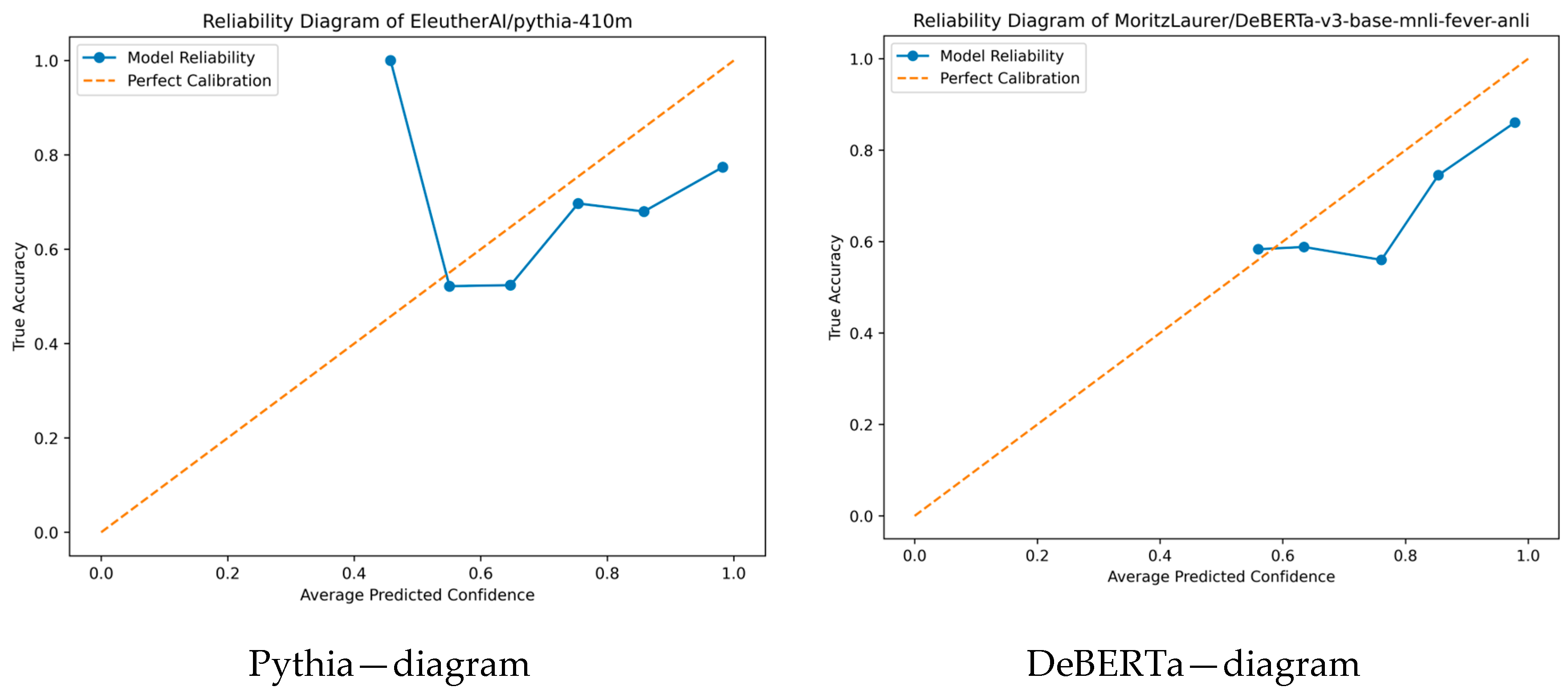
In climate_3cl, we have the winner, MV-“T5,GPT2,Pythia” and the second place, SV-”DeBERTa,T5,GPT2”, so we will consider the four different models, T5, GPT2, Pythia and DeBERTa, which are the basic models of the sets. The last two, Pythia and DeBERTa, are the ones that are not common to the two ensemble schemes, and we will consider them first, because Pythia has more characteristic sets of predictions (bins) which makes it easier to explain.

The confidence graph evaluates the accuracy of the model’s confidence after training. The meaningful information is in the bins (blue dots), which group predictions with similar confidence levels. Each bin represents a set of predictions of the model, where its coordinates (x, y) have a specific meaning.

The x-axis indicates the average probability predicted by the model for that particular group, while the y-axis shows the actual Accuracy of the predictions of that group. For example, in Pythia’s reliability diagram, Figure 1, the first bin on the left is a group of predictions that have the following characteristics:

The model predicts with a confidence of 0.4–0.5; that is, it is quite uncertain about these predictions. The actual Accuracy in this group is close to 0.99. This means that almost all of these predictions are correct. So, the model underestimates its capabilities in these cases. So, this bin contains predictions where the model should be much more confident, but is not (underconfidence).

In general, if the points are above the dotted line, then the model is underconfident, whereas if the points are below the dotted line, the model is overconfident, displaying too much confidence in predictions that are less correct than it thinks (overconfidence in incorrect answers). If the model were perfectly calibrated, then the points would fall on the dotted line (perfect calibration: p (confidence) = p (accuracy)), Figure 1 and Figure 2.

We compiled the results of the charts into a table with three metrics:

Average confidence (correct): shows the average confidence of predictions that are correct. The higher this value is, the higher the confidence of the model when making correct predictions. A very high value here is usually desirable, as it means that the model is confident when it is correct.

Average confidence (incorrect): shows the average confidence of incorrect predictions. A high value for this would suggest that the model is often overconfident even when it makes an error, i.e., the model is not very well-calibrated. This should ideally be much lower than that of correct predictions, so that correct and incorrect predictions can be easily distinguished.

The Expected Calibration Error (ECE) is a metric that assesses how well-calibrated the confidence of a model’s predictions is. The ideal forecast has high confidence when it is correct and low confidence when it is incorrect. ECE is calculated by grouping forecasts into confidence intervals (bins) and comparing the average confidence of each bin to its actual Accuracy. The lower the ECE, the better the confidence rating of the model.

As we can observe from the analysis of the climate_3cl dataset in

Table 16. Calibration metrics for climate_3cl Models.

Model	Average Confidence (Correct)	Average Confidence (Incorrect)	ECE
climate_3cl/Pythia	0.9256	0.8672	0.1807
climate_3cl/DeBERTa	0.9340	0.8611	0.1157
climate_3cl/GPT-2	0.9129	0.8116	0.0894
climate_3cl/T5	0.9372	0.8598	0.1092

, the average confidence of all models in correct prediction is high, from 0.9129 for GPT2 to 0.9372 for T5. Both DeBERTa and T5 have maximum confidence in correct prediction, but GPT2 has minimum confidence, i.e., this model is less confident in its estimate. In the incorrect predictions, confidence is also high but lower than in the correct predictions, from 0.8116 (GPT2) to 0.8672 (Pythia). In GPT2, the difference between confidence in correct and incorrect predictions is greater, showing that the model can better discriminate its predictions based on correctness. When compared on the basis of ECE value, GPT2 achieves the optimal calibration of 0.0894 and its predictions are the best-calibrated among the four models. T5 and DeBERTa have slightly higher ECE values (0.1092 and 0.1157, respectively), while Pythia shows the worst rating with an ECE of 0.1807, suggesting that its confidence often deviates from the actual Accuracy of predictions. Overall, GPT2 appears to be the most reliable in terms of confidence rating, while Pythia shows the largest deviation, suggesting that it may be overconfident in its estimates even when it is wrong.

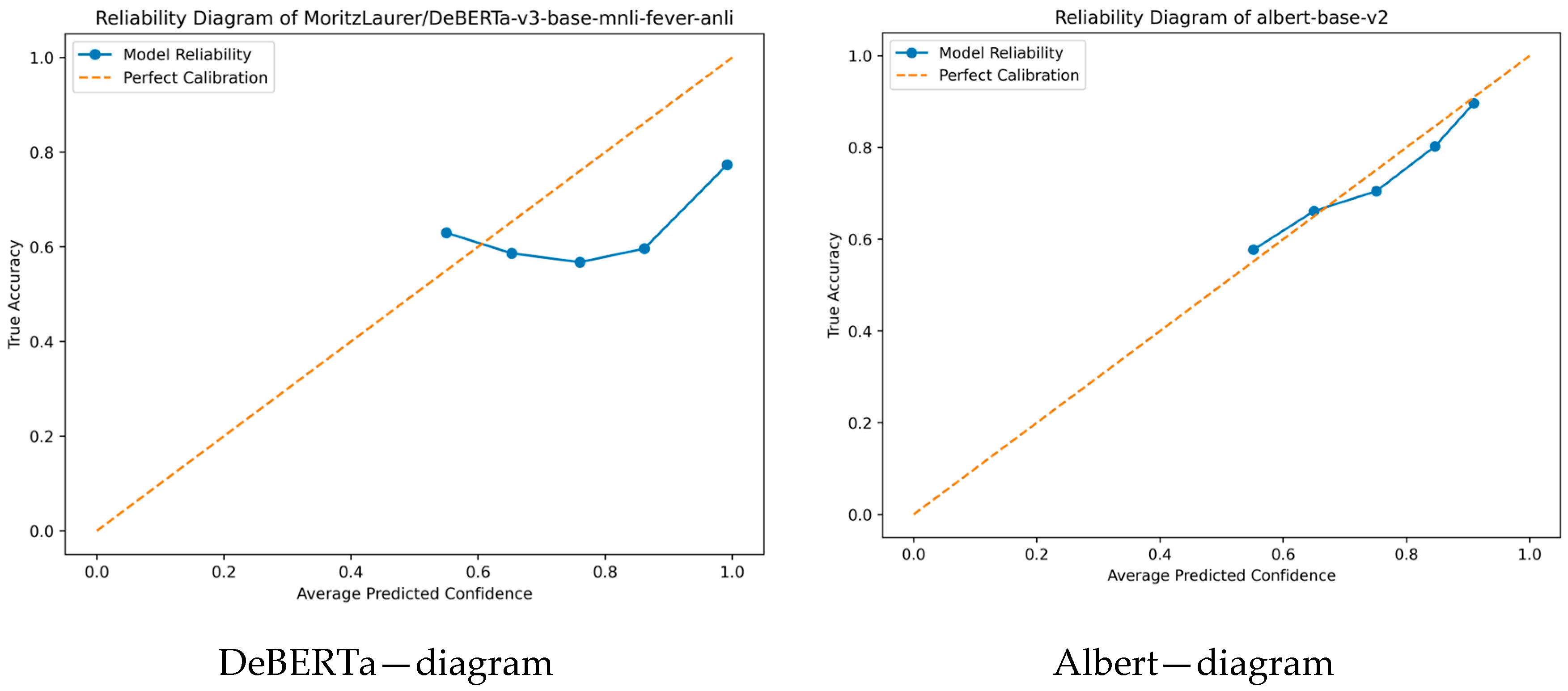
In cardiffnlp_2cl, we have MV-“DeBERTa,Albert,Pythia” as the winner, followed by DeBERTa in second place, and a very close marginal third place is SV-“DeBERTa,Albert,GPT2”, so we will consider the four different models, DeBERTa, Albert, Pythia and GPT2, which are the base models of the ensembles as illustrated in Figure 3 and in Figure 4.

In the analysis of results, we observe that there are significant variations between the models in their confidence in correct and incorrect predictions, and in calibration to the ECE measure as illustrated in

Table 17. Calibration Metrics for cardifnlp_2cl Models.

Model	Average Confidence (Correct)	Average Confidence (Incorrect)	ECE
cardifnlp_2cl/DeBERTa	0.9719	0.9441	0.2138
cardifnlp_2cl/Albert	0.7252	0.6783	0.0325
cardifnlp_2cl/Pythia	0.7066	0.6626	0.0420
cardifnlp_2cl/GPT2	0.7941	0.7283	0.0937

.

The DeBERTa model has the highest correct (0.9719) and incorrect average confidence (0.9441). This indicates the model is nearly always very confident in its predictions, both when it is correct and when it is incorrect. However, the high ECE value (0.2138) indicates that the model is poorly calibrated because the confidence does not reflect the actual performance.

On the other hand, Albert and Pythia have significantly lower average confidence in both correct and incorrect predictions. Albert has an average e-confidence of 0.7252 in correct and 0.6783 in incorrect predictions, while Pythia has 0.7066 and 0.6626, respectively. The small difference between these values shows that these models are conservative in their estimations, giving more balanced confidence values. This is evident in the extremely low values of ECE (0.0325 for Albert and 0.0420 for Pythia), which point to the fact that they are the best-calibrated models among the compared models.

GPT2 is more certain, with 0.7941 for correct and 0.7283 for incorrect predictions. GPT2 is less certain than DeBERTa but more certain than Albert and Pythia. GPT2’s ECE (0.0937) is lower than Albert and Pythia but much lower than DeBERTa, which shows its calibration is better than DeBERTa but bad in comparison to the other two models.

Overall, if the criterion is better calibration, Albert and Pythia excel, as they have lower ECE and more balanced confidence values. GPT2 is in the middle, while DeBERTa, although having the highest confidence values, has a poor rating due to its high ECE, which means that it can be overconfident even when wrong.

4.3. Final Results—Average Metric Values

By using ensembles, we maximized the performance compared to the first six models, but we still need to come up with a scheme that is the ultimate winner. We first calculated the average values of the metrics. That is, for each classifier we summed the metric scores for each dataset and then divided it by the total dataset.

Table 18. Average metric values of all classifiers.

No	Classifiers	Accuracy Mean	F1-Score Mean	Precision Mean	Recall Mean	MCC Mean	Kappa Mean
1	MV-DeBERTa,Albert,GPT2	0.896	0.896	0.898	0.896	0.817	0.816
2	MV-DeBERTa,T5,GPT2	0.895	0.895	0.897	0.895	0.815	0.814
3	MV-DeBERTa,T5,Albert	0.894	0.894	0.897	0.894	0.814	0.813
4	MV-DeBERTa,Albert,Pythia	0.894	0.894	0.896	0.894	0.814	0.813
5	MV-DeBERTa,GPT2,Pythia	0.894	0.894	0.896	0.894	0.814	0.813
6	MV-DeBERTa,T5,Pythia	0.892	0.892	0.894	0.892	0.810	0.809
7	MV-T5,Albert,GPT2	0.889	0.889	0.892	0.889	0.805	0.803
8	MV-Bart,Albert,GPT2	0.888	0.888	0.891	0.888	0.805	0.802
9	MV-T5,Albert,Pythia	0.888	0.887	0.891	0.888	0.803	0.801
10	MV-T5,GPT2,Pythia	0.887	0.887	0.890	0.887	0.803	0.800
11	MV-Bart,T5,GPT2	0.886	0.885	0.888	0.886	0.802	0.799
12	MV-Bart,T5,Albert	0.886	0.885	0.888	0.886	0.801	0.799
13	MV-Bart,Albert,Pythia	0.886	0.885	0.889	0.886	0.802	0.800
14	MV-Bart,GPT2,Pythia	0.886	0.885	0.888	0.886	0.801	0.799
15	MV-Bart,DeBERTa,GPT2	0.884	0.884	0.886	0.884	0.798	0.796
16	MV-Bart,T5,Pythia	0.883	0.883	0.886	0.883	0.798	0.795
17	MV-Bart,DeBERTa,Albert	0.883	0.882	0.885	0.883	0.796	0.794
18	MV-Bart,DeBERTa,T5	0.883	0.882	0.885	0.883	0.795	0.793
19	MV-Bart,DeBERTa,Pythia	0.880	0.880	0.882	0.880	0.791	0.789
20	MV-Albert,GPT2,Pythia	0.873	0.873	0.875	0.873	0.773	0.772
21	SV-Bart,DeBERTa,T5	0.863	0.862	0.862	0.862	0.759	0.759
22	SV-DeBERTa,T5,GPT2	0.861	0.858	0.861	0.858	0.754	0.753
23	SV-Bart,DeBERTa,GPT2	0.860	0.858	0.86	0.857	0.754	0.753
25	SV-Bart,DeBERTa,Albert	0.859	0.856	0.86	0.854	0.752	0.751
24	SV-DeBERTa,T5,Albert	0.859	0.857	0.86	0.854	0.753	0.753
26	SV-DeBERTa,T5,Pythia	0.858	0.854	0.858	0.853	0.748	0.747
27	SV-DeBERTa,Albert,GPT2	0.857	0.854	0.858	0.853	0.748	0.747
28	SV-Bart,DeBERTa,Pythia	0.857	0.854	0.858	0.851	0.747	0.746
29	DeBERTa	0.855	0.854	0.854	0.851	0.745	0.744
30	SV-Bart,T5,GPT2	0.854	0.852	0.854	0.851	0.742	0.742
31	SV-Bart,T5,Albert	0.854	0.851	0.853	0.847	0.742	0.742
32	SV-DeBERTa,GPT2,Pythia	0.853	0.849	0.852	0.847	0.74	0.739
33	SV-DeBERTa,Albert,Pythia	0.852	0.848	0.850	0.845	0.739	0.737
34	SV-T5,Albert,GPT2	0.850	0.847	0.849	0.845	0.735	0.734
35	SV-Bart,T5,Pythia	0.850	0.847	0.849	0.845	0.734	0.734
36	SV-Bart,Albert,GPT2	0.849	0.846	0.848	0.841	0.734	0.733
37	SV-T5,Albert,Pythia	0.847	0.845	0.848	0.839	0.729	0.727
38	SV-T5,GPT2,Pythia	0.847	0.845	0.847	0.838	0.728	0.727
39	T5	0.845	0.843	0.845	0.838	0.728	0.727
40	Bart	0.845	0.842	0.842	0.838	0.727	0.726
41	SV-Bart,Albert,Pythia	0.844	0.840	0.841	0.836	0.725	0.723
42	SV-Bart,GPT2,Pythia	0.843	0.840	0.838	0.828	0.722	0.721
43	SV-Albert,GPT2,Pythia	0.839	0.832	0.831	0.827	0.714	0.712
44	GPT2	0.832	0.831	0.818	0.816	0.704	0.703
45	Albert	0.827	0.826	0.818	0.809	0.695	0.693
46	Pythia	0.803	0.799	0.800	0.768	0.650	0.645

presents all the average values of the metrics for the set of classifiers. From this table, we can decide the winner over all datasets and make a general estimate of which ensemble shape is the winner on average over all datasets. But is this classifier (DeBERTa,Albert,GPT2) the undisputed winner?

It is obviously not the undisputed winner, we shall see why shortly. Following, in

Table 19. Friedman ranking.

Model	MV_Accuracy_Avg_F-Rank	SV_Accuracy_Avg_F-Rank
DeBERTa,T5,GPT2	5.333333	5.833333
DeBERTa,Albert,GPT2	5.666667	8.500000
DeBERTa,T5,Albert	6.750000	6.083333
DeBERTa,GPT2,Pythia	7.250000	12.833333
DeBERTa,Albert,Pythia	7.750000	13.250000
DeBERTa,T5,Pythia	8.083333	7.750000
Bart,Albert,GPT2	8.916667	14.583333
T5,Albert,GPT2	9.000000	13.750000
T5,Albert,Pythia	9.583333	17.500000
T5,GPT2,Pythia	9.916667	17.333333
Bart,T5,GPT2	10.750000	10.916667
Bart,Albert,Pythia	11.083333	18.583333
Bart,GPT2,Pythia	11.333333	19.833333
Bart,T5,Albert	11.416667	9.333333
Bart,DeBERTa,GPT2	12.000000	5.666667
Bart,DeBERTa,T5	13.833333	3.083333
Bart,T5,Pythia	14.083333	13.833333
Bart,DeBERTa,Albert	14.416667	5.083333
Bart,DeBERTa,Pythia	16.916667	8.500000
Albert,GPT2,Pythia	18.916667	22.333333
DeBERTa	19.416667	10.583333
Bart	22.166667	17.916667
T5	22.416667	15.833333
GPT2	23.500000	22.000000
Albert	24.583333	24.166667
Pythia	25.916667	25.916667

we present the Friedman ranking for the Majority and Soft vote. The Friedman ranking calculates the average position of each model on multiple datasets, and the lower the value, the better the model performs compared to the others.

The analysis of the average ranking with Friedman ranking shows that the scheme “DeBERTa, T5, GPT2” has the best performance, as it shows the lowest average ranking in Majority vote (5.333333, second column in Table 19). The others have higher values, which means that on average they rank lower.

However, the use of the Nemenyi test for statistical comparison of the models reveals that the maximum difference between the top 18 rankings in the Majority vote (and top 16 rankings in the Soft vote) is smaller than the critical difference (CD = 10.802). This implies that the differences in performance between the models are not statistically significant at a significance level of α = 0.10, suggesting that the models have comparable performance and that the differences may be due to randomness. According to Demšar (2006) [44], the Nemenyi test is used for multiple comparisons after the Friedman test, and when the differences do not exceed the critical value, we cannot claim that one model is objectively superior to the others.

5. Conclusions

In our research study, we evaluated the performance of different classifiers based on Majority vote and Soft vote and also calibrated the models to study their confidence in the predictions. The results showed that the Majority vote method outperforms both the Soft vote and the individual models. This is particularly true for unbalanced data and data containing linguistic idiosyncrasies such as irony. The Soft vote method, however, is better for more balanced data, but is still more vulnerable to models with overconfidence in their predictions. The results showed that some of the models, such as DeBERTa and T5, are overconfident in their predictions, even for predictions that are wrong. This resulted in a larger Expected Calibration Error (ECE), which affects the probability-based Soft vote. Majority vote, which is based on classes only, was less exposed to this trend. Although the “DeBERTa, T5, GPT2” system recorded the highest average performance in the Accuracy, F1-score, Precision, Recall and MCC metrics, statistical analyses with Friedman ranking and Nemenyi test showed that the differences between the top combinations were not statistically significant. This means that, despite small differences in performance, most of the ensemble schemes had similar effectiveness.

The results show that using different models in a set reduces errors and biases, but the way in which they are combined plays a critical role. Soft vote requires properly tuned models to work correctly, while Majority vote offers greater stability, especially on difficult datasets. One main question that arises is whether to train models to high accuracy at the expense of overconfidence or whether to terminate training earlier for more generalization. This trade-off influences the selection of the most suitable ensemble and can account for why Majority vote often wins, as it is less sensitive to probability calibration. This study confirms that ensemble models are an effective strategy for sentiment analysis, with Majority vote being the most reliable choice in most scenarios. However, the importance of calibration and overconfidence of the models are critical factors for the correct selection and combination of classifiers. Future research could focus on more advanced model calibration techniques to further boost the performance of Soft vote, and other classifier combination techniques to achieve higher accuracy and generalization. One potential conclusion of the Nemenyi test is that the variation between the performance of the ensemble models is not sufficiently significant as to be statistically distinct.

This may be due to several reasons: The transformers used are high-performance and share a similar natural language processing capacity. There are minor differences, but they are not big enough to result in an observable gap between them. Model combinations have common members (e.g., DeBERTa, GPT2, T5), which may reduce the difference in their performance. If the classifiers were more diverse (e.g., models from different architectures), there might be more divergence. However, we cannot avoid this because we have chosen all possible combinations of triads from six models, so we must have common members. The results come from different datasets, and there may be a strong dependence between ensemble performance and dataset characteristics. In some datasets, an ensemble would be superior, and in others it can be as good as the others. This is an average-based statistical test that may not catch small differences which may make a significant practical difference. It could be done differently using different methods, e.g., by bootstrap confidence intervals or Bayesian estimation. Therefore, the main message that emerges is that the Majority vote ensemble is the undisputed winner; there is no clear “best” ensemble model, but rather different combinations that are equivalent in performance. This suggests that the ensemble choice may be more dependent on the particular dataset and application.

References

1. Liapis, C.M.; Kyritsis, K.; Perikos, I.; Spatiotis, N.; Paraskevas, M. A Hybrid Ensemble Approach for Greek Text Classification Based on Multilingual Models. Big Data Cogn. Comput. 2024, 8, 137. [Google Scholar] [CrossRef]
2. Wang, J.-H.; Norouzi, M.; Tsai, S.M. Augmenting Multimodal Content Representation with Transformers for Misinformation Detection. Big Data Cogn. Comput. 2024, 8, 134. [Google Scholar] [CrossRef]
3. Haque, R.; Islam, N.; Tasneem, M.; Das, A.K. Multi-Class Sentiment Classification on Bengali Social Media Comments Using Machine Learning. Int. J. Cogn. Comput. Eng. 2023, 4, 21–35. [Google Scholar] [CrossRef]
4. Areshey, A.; Mathkour, H. Exploring Transformer Models for Sentiment Classification: A Comparison of BERT, RoBERTa, ALBERT, DistilBERT, and XLNet. Expert Syst. 2024, 41, e13701. [Google Scholar] [CrossRef]
5. Singla, S.; Ramachandra, N. Comparative Analysis of Transformer Based Pre-Trained NLP Models. Int. J. Comput. Sci. Eng. 2020, 8, 40–44. [Google Scholar]
6. Michailidis, P.D. A Comparative Study of Sentiment Classification Models for Greek Reviews. Big Data Cogn. Comput. 2024, 8, 107. [Google Scholar] [CrossRef]
7. Ashbaugh, L.; Zhang, Y. A Comparative Study of Sentiment Analysis on Customer Reviews Using Machine Learning and Deep Learning. Computers 2024, 13, 340. [Google Scholar] [CrossRef]
8. Alotaibi, A.; Nadeem, F. Leveraging Social Media and Deep Learning for Sentiment Analysis for Smart Governance: A Case Study of Public Reactions to Educational Reforms in Saudi Arabia. Computers 2024, 13, 280. [Google Scholar] [CrossRef]
9. Ali, H.; Hashmi, E.; Yayilgan Yildirim, S.; Shaikh, S. Analyzing Amazon Products Sentiment: A Comparative Study of Machine and Deep Learning, and Transformer-Based Techniques. Electronics 2024, 13, 1305. [Google Scholar] [CrossRef]
10. Radecki, A.; Rybicki, T. Comparison of Sentiment Analysis Methods Used to Investigate the Quality of Teaching Aids Based on Virtual Simulators of Embedded Systems. Electronics 2024, 13, 1811. [Google Scholar] [CrossRef]
11. Cui, S.; Han, Y.; Duan, Y.; Li, Y.; Zhu, S.; Song, C. A Two-Stage Voting-Boosting Technique for Ensemble Learning in Social Network Sentiment Classification. Entropy 2023, 25, 555. [Google Scholar] [CrossRef]
12. Wan, Y.; Gao, Q. An Ensemble Sentiment Classification System of Twitter Data for Airline Services Analysis. In Proceedings of the 2015 IEEE International Conference on Data Mining Workshop (ICDMW), Atlantic City, NJ, USA, 14–17 November 2015; IEEE: Piscataway, NJ, USA, 2015; pp. 1318–1325. [Google Scholar]
13. Wolf, T.; Debut, L.; Sanh, V.; Chaumond, J.; Delangue, C.; Moi, A.; Cistac, P.; Rault, T.; Louf, R.; Funtowicz, M.; et al. HuggingFace’s Transformers: State-of-the-Art Natural Language Processing. arXiv 2020, arXiv:1910.03771. [Google Scholar]
14. Howard, J.; Ruder, S. Universal Language Model Fine-Tuning for Text Classification. arXiv 2018, arXiv:1801.06146. [Google Scholar]
15. Lewis, M.; Liu, Y.; Goyal, N.; Ghazvininejad, M.; Mohamed, A.; Levy, O.; Stoyanov, V.; Zettlemoyer, L. BART: Denoising Sequence-to-Sequence Pre-Training for Natural Language Generation, Translation, and Comprehension. arXiv 2019, arXiv:1910.13461. [Google Scholar]
16. He, P.; Liu, X.; Gao, J.; Chen, W. DeBERTa: Decoding-Enhanced BERT with Disentangled Attention. arXiv 2021, arXiv:2006.03654. [Google Scholar]
17. He, P.; Gao, J.; Chen, W. DeBERTaV3: Improving DeBERTa Using ELECTRA-Style Pre-Training with Gradient-Disentangled Embedding Sharing. arXiv 2023, arXiv:2111.09543. [Google Scholar]
18. Radford, A.; Wu, J.; Child, R.; Luan, D.; Amodei, D.; Sutskever, I. Language Models Are Unsupervised Multitask Learners. OpenAI Blog 2019, 1, 9. [Google Scholar]
19. Biderman, S.; Schoelkopf, H.; Anthony, Q.; Bradley, H.; O’Brien, K.; Hallahan, E.; Khan, M.A.; Purohit, S.; Prashanth, U.S.; Raff, E.; et al. Pythia: A Suite for Analyzing Large Language Models Across Training and Scaling. arXiv 2023, arXiv:2304.01373. [Google Scholar]
20. Black, S.; Biderman, S.; Hallahan, E.; Anthony, Q.; Gao, L.; Golding, L.; He, H.; Leahy, C.; McDonell, K.; Phang, J.; et al. GPT-NeoX-20B: An Open-Source Autoregressive Language Model. arXiv 2022, arXiv:2204.06745. [Google Scholar]
21. Raffel, C.; Shazeer, N.; Roberts, A.; Lee, K.; Narang, S.; Matena, M.; Zhou, Y.; Li, W.; Liu, P.J. Exploring the Limits of Transfer Learning with a Unified Text-to-Text Transformer. arXiv 2023, arXiv:1910.10683. [Google Scholar]
22. Lan, Z.; Chen, M.; Goodman, S.; Gimpel, K.; Sharma, P.; Soricut, R. ALBERT: A Lite BERT for Self-Supervised Learning of Language Representations. arXiv 2020, arXiv:1909.11942. [Google Scholar]
23. Causal Language Modeling. Available online: https://huggingface.co/docs/transformers/tasks/language_modeling (accessed on 1 February 2025).
24. Devlin, J.; Chang, M.-W.; Lee, K.; Toutanova, K. BERT: Pre-Training of Deep Bidirectional Transformers for Language Understanding. arXiv 2018, arXiv:1810.04805. [Google Scholar] [CrossRef]
25. Sokolova, M.; Lapalme, G. A Systematic Analysis of Performance Measures for Classification Tasks. Inf. Process. Manag. 2009, 45, 427–437. [Google Scholar] [CrossRef]
26. Baeza-Yates, R.; Ribeiro-neto, B.; Mills, D.; Bonn, O.; Juan, S.; Mexico, M.; Taipei, C.; Wesley, A.; Limited, L. Modern Information Retrieval; Association for Computing Machinery: New York, NY, USA, 1999. [Google Scholar]
27. Sasaki, Y. The Truth of the F-Measure. Teach Tutor Mater 2007, 1, 1–5. [Google Scholar]
28. Chicco, D.; Jurman, G. The Advantages of the Matthews Correlation Coefficient (MCC) over F1 Score and Accuracy in Binary Classification Evaluation. BMC Genom. 2020, 21, 6. [Google Scholar] [CrossRef]
29. Cohen, J. A Coefficient of Agreement for Nominal Scales. Educ. Psychol. Meas. 1960, 20, 37–46. [Google Scholar] [CrossRef]
30. Lakshminarayanan, B.; Pritzel, A.; Blundell, C. Simple and Scalable Predictive Uncertainty Estimation Using Deep Ensembles. arXiv 2017, arXiv:1612.01474. [Google Scholar]
31. Guo, C.; Pleiss, G.; Sun, Y.; Weinberger, K.Q. On Calibration of Modern Neural Networks. arXiv 2017, arXiv:1706.04599. [Google Scholar]
32. Kittler, J.; Hatef, M.; Duin, R.P.W.; Matas, J. On Combining Classifiers. IEEE Trans. Pattern Anal. Mach. Intell. 1998, 20, 226–239. [Google Scholar] [CrossRef]
33. Dietterich, T.G. Ensemble Methods in Machine Learning. In Proceedings of the Multiple Classifier Systems, Cagliari, Italy, 21–23 June 2000; Springer: Berlin/Heidelberg, Germany, 2000; pp. 1–15. [Google Scholar]
34. Maclin, R.; Opitz, D. Popular Ensemble Methods: An Empirical Study. J. Artif. Intell. Res. 1999, 11, 169–198. [Google Scholar] [CrossRef]
35. Gupta, N.; Smith, J.; Adlam, B.; Mariet, Z. Ensembling over Classifiers: A Bias-Variance Perspective. arXiv 2022, arXiv:2206.10566. [Google Scholar]
36. Kumar, A.N.; Prashanth, C.; Kumar, L.C.; Sridhar, A. A Hybrid Approach to Credit Card Fraud Detection: Integrating Adaboost and Majority Voting for Enhanced Accuracy and Robustness. Front. Collab. Res. 2024, 2, 51–58. [Google Scholar]
37. Cheng, J.; Huang, L.; Tang, B.; Wu, Q.; Wang, M.; Zhang, Z. A Minority Sample Enhanced Sampler for Crop Classification in Unmanned Aerial Vehicle Remote Sensing Images with Class Imbalance. Agriculture 2025, 15, 388. [Google Scholar] [CrossRef]
38. Smith, M.R.; Martinez, T. The Robustness of Majority Voting Compared to Filtering Misclassified Instances in Supervised Classification Tasks. Artif. Intell. Rev. 2018, 49, 105–130. [Google Scholar] [CrossRef]
39. Khurana, U.; Nalisnick, E.; Fokkens, A.; Swayamdipta, S. Crowd-Calibrator: Can Annotator Disagreement Inform Calibration in Subjective Tasks? arXiv 2024, arXiv:2408.14141. [Google Scholar]
40. Taha, A. Intelligent Ensemble Learning Approach for Phishing Website Detection Based on Weighted Soft Voting. Mathematics 2021, 9, 2799. [Google Scholar] [CrossRef]
41. DeVries, T.; Taylor, G.W. Learning Confidence for Out-of-Distribution Detection in Neural Networks. arXiv 2018, arXiv:1802.04865. [Google Scholar]
42. Minderer, M.; Djolonga, J.; Romijnders, R.; Hubis, F.; Zhai, X.; Houlsby, N.; Tran, D.; Lucic, M. Revisiting the Calibration of Modern Neural Networks. arXiv 2021, arXiv:2106.07998. [Google Scholar]
43. Niculescu-Mizil, A.; Caruana, R. Predicting Good Probabilities with Supervised Learning. In Proceedings of the 22nd International Conference on Machine Learning-ICML ’05, Bonn, Germany, 7–11 August 2005; ACM Press: New York, NY, USA, 2005; pp. 625–632. [Google Scholar]
44. Demšar, J. Statistical Comparisons of Classifiers over Multiple Data Sets. J. Mach. Learn. Res. 2006, 7, 1–30. [Google Scholar]
Figure 1. Reliability diagrams of Pythia and DeBERTa in the climate_3cl dataset. The dotted diagonal line represents perfect calibration; points above it indicate underconfidence, below indicate overconfidence.
Computers 14 00167 g001
Figure 2. Reliability plots of T5 and GPT2 in the climate_3cl dataset. The diagonal line shows perfect calibration, the two plots show similar behavior; points above the line indicate underconfidence, points below indicate overconfidence.
Computers 14 00167 g002
Figure 3. Reliability diagrams of DeBERTa and Albert in cardiffnlp_2cl dataset; points above the dotted line indicate underconfidence, points below indicate overconfidence. Albert has almost perfect calibration.
Computers 14 00167 g003
Figure 4. Reliability diagrams of Pythia and GPT2 in the cardiffnlp_2cl dataset; points above the dotted line indicate underconfidence, points below indicate overconfidence.
Computers 14 00167 g004