Fine-Tuning Network Slicing in 5G: Unveiling Mathematical Equations for Precision Classification

Abstract

Modern 5G network slicing centers on the precise design of virtual, independent networks operating over a shared physical infrastructure, each configured to meet specific service requirements. This approach plays a vital role in enabling highly customized and flexible service delivery within the 5G ecosystem. In this study, we present the application of a genetic programming symbolic classifier to a dedicated network slicing dataset, resulting in the generation of accurate symbolic expressions for classifying different network slice types. To address the issue of class imbalance, we employ oversampling strategies that produce balanced variations of the dataset. Furthermore, a random search strategy is used to explore the hyperparameter space comprehensively in pursuit of optimal classification performance. The derived symbolic models, refined through threshold tuning based on prediction correctness, are subsequently evaluated on the original imbalanced dataset. The proposed method demonstrates outstanding performance, achieving a perfect classification accuracy of 1.0.

1. Introduction

Network slicing is a transformative architectural concept that plays a central role in the development of 5G technology [1]. Unlike traditional network designs, it enables the virtualization and segmentation of a physical network into multiple independent entities known as slices [2]. Each slice functions as a customized network instance, optimized to meet the unique requirements of different services, applications, or industries [3]. This approach allows isolated environments to coexist on the same infrastructure, each with dedicated resources and configurations tailored to specific use cases.

These slices operate independently, ensuring that the performance, security, and functionality of one slice do not affect the others [4]. Customization encompasses a wide range of parameters, such as latency, bandwidth, reliability, and security [5]. This flexibility allows operators to dynamically allocate resources based on changing workloads, enhancing both efficiency and responsiveness.

Network slicing is particularly valuable for supporting the diverse range of services enabled by 5G. It provides tailored support for use cases such as enhanced Mobile Broadband (eMBB), massive machine-type communication (mMTC), and Ultra-Reliable Low-Latency Communication (URLLC) [6]. Moreover, it addresses the complex needs of emerging sectors, including the Internet of Things (IoT), smart cities, and healthcare systems [1].

In summary, network slicing represents a significant advancement in telecommunications, offering a flexible and efficient means to deliver a wide array of services over shared physical infrastructures. It is a foundational component of 5G networks and plays a crucial role in the broader evolution of digital connectivity.

The integration of artificial intelligence (AI) with network slicing in 5G networks opens new possibilities for creating intelligent, adaptive, and self-optimizing telecommunications infrastructures [7]. AI significantly enhances network slicing by enabling 5G networks to dynamically adapt to varying service requirements [6].

A key advantage of this integration is AI’s ability to drive dynamic resource allocation [8]. Through real-time analysis of network conditions, traffic patterns, and application demands, AI algorithms can efficiently manage the distribution of resources among network slices. This ensures that each slice receives the appropriate resources, minimizing latency and maximizing bandwidth according to real-time service demands [9].

AI-driven predictive analytics further enhance slice management [10]. By forecasting traffic trends and anticipating demand fluctuations, AI can preemptively adjust resource allocations, which is particularly useful during unexpected surges [11].

In addition to allocation, AI supports ongoing optimization and monitoring of slice performance. Algorithms continuously assess key parameters—such as quality of service (QoS), security, and routing—and make real-time adjustments to enhance efficiency and reliability [12].

AI also strengthens network security by using intelligent detection systems to monitor for anomalies and potential threats. These systems enable automated, self-healing responses to security incidents [13,14], thereby improving the overall robustness of the network.

Together, AI and network slicing significantly enhance the intelligence and flexibility of 5G infrastructures. This integration enables networks to not only respond to current demands but also anticipate and prepare for future challenges.

In [15], the authors applied various machine learning models—including logistic regression (LR), the linear discriminant model (LDM), k-nearest neighbors (k-NN), the decision tree classifier (DTC), the random forest classifier (RFC), the support vector classifier (SVC), Gaussian Naive Bayes (GNB), and artificial neural networks (ANNs)—for network slice detection. LR, k-NN, DTC, RFC, and SVC all achieved perfect classification scores, with accuracy, precision, recall, and F1-score metrics all equal to 1.0.

The DeepSlice model, introduced in [16], employs deep neural networks (DNNs) to manage network load and availability via in-network deep learning and prediction. The best-trained model achieved an accuracy of 0.95 on both the training and testing sets.

DeepSecure, presented in [17], utilizes Long Short-Term Memory (LSTM) networks to detect distributed denial-of-service (DDoS) attacks on network slices. Unlike traditional methods based on statistical or cryptographic techniques, DeepSecure provides a low-overhead, AI-driven approach that achieves an accuracy of 0.9997 in DDoS detection and 0.9879 in predicting the appropriate slices for legitimate requests.

In [18], models such as k-NN, Naive Bayes, SVC, RFC, and Multi-Layer Perceptron (MLP) were used for slice type detection. MLP with the ADAM optimizer achieved the highest performance across all three slice types, with accuracy, precision, recall, and F1-score values of 0.98.

Finally in [19], the authors have explored the use of SVC, RFC, DTC, and ANN—with and without feature selection—for predicting optimal slices. The ANOVA + ANN model demonstrated superior performance (accuracy = 0.9446, precision = 0.9425, recall = 0.9361, F1-score = 0.9288), highlighting the significance of network function virtualization and software-defined networking in enhancing slice performance.

All the results obtained in previous research are summarized in

Table 1. The summarized results achieved in previous research.

Reference	AI Methods	Classification Performance
[15]	LR, LDM, KNN, DTC, RFC, SVC, GNB	ACC = 1.0
[16]	DeepSlice (DNN)	ACC = 0.95
[17]	DeepSecure (LSTM)	ACC = 0.98798
[18]	k-NN, NB, SVC, RFC, MLP	ACC = 0.98 Precision = 0.98 Recall = 0.98 F1-Score = 0.98
[19]	SVC, RFC, DTC, and ANN	ACC = 0.9446 Precision = 0.9425 Recall = 0.9361 F1-score = 0.9288

.

As shown in Table 1, recent studies in network slicing classification largely rely on diverse artificial intelligence (AI) techniques. While many of these methods achieve impressive accuracy, a common limitation is their inability to generate concise symbolic expressions (SEs) or interpretable mathematical equations. This issue is particularly evident in models such as artificial neural networks (ANNs) and deep neural networks (DNNs), where the complexity of interconnected neurons prevents straightforward transformation into simple SEs.

However, this limitation is not exclusive to ANNs or DNNs; it also affects several other AI techniques listed in Table 1. In addition to their interpretability challenges, many of these models require significant computational resources—including high memory usage, CPU/GPU demands, and storage capacity—for both training and inference. In contrast, models that produce simple SEs offer substantial advantages: they are lightweight, require minimal memory, and impose low computational overhead when applied to new data. This highlights the trade-off between accuracy and practical concerns such as interpretability and resource efficiency when selecting AI methods for network slicing classification.

This study introduces the Genetic Programming Symbolic Classifier (GPSC) as a method for deriving symbolic expressions that effectively classify network slices. One of the key benefits of the GPSC is that once the model is trained, the resulting symbolic expressions (SEs) can be directly applied, eliminating the need to store and reload the model—unlike techniques such as Multi-Layer Perceptrons (MLPs), where model complexity hinders easy reuse in symbolic form. Furthermore, the simplicity of SEs leads to minimal computational costs during deployment. To improve classification performance, a Random Hyperparameter Value Search (RHVS) strategy will be developed, aimed at identifying the optimal combinations of GPSC hyperparameters to enhance the accuracy of the SEs. The study will also employ 5-fold cross-validation (5FCV) to generate a robust set of symbolic expressions. In light of the class imbalance in the original dataset, various oversampling methods will be explored to create balanced dataset variants, which will then be used to train the GPSC and generate more effective symbolic expressions. Based on the literature and the proposed approach, the following questions emerge:

• Is it possible to obtain highly accurate SEs using the GPSC that can be used to determine the network slice class type with high classification accuracy?
• Does the oversampling technique have any influence on the accuracy of obtained SEs?
• Can the RHVS method be used to find the optimal combination of GPSC hyperparameters with which mathematical equations could be obtained with high classification accuracy?
• Using 5FCV, is it possible to obtain highly accurate and robust SEs for the detection of network slicing type?
• Can a combination of all the best SEs for each class applied on an initial imbalanced dataset achieve the same or similar classification accuracy as those SEs achieve on balanced dataset variations?

This paper is organized into the following key sections: Section 2, Section 3, Section 4, and Section 5. The Section 2 starts with both a graphical and descriptive overview of the proposed research methodology. It continues with a detailed analysis of the dataset, including statistical insights, an explanation of the applied oversampling techniques, the introduction of the Genetic Programming Symbolic Classifier (GPSC) and the Random Hyperparameter Value Search (RHVS) method, followed by the evaluation metrics and the procedure for training and testing.

In the Section 3, the symbolic expressions (SEs) that provided the highest classification performance are presented. This section also discusses the performance of these SEs when applied to the original imbalanced dataset.

The Section 4 offers a thorough examination of the entire process, from dataset preparation to result interpretation. The results are critically compared with the existing literature to emphasize the contributions and advancements made by the proposed approach.

The Section 5 provides a concise summary of the research objectives and accomplishments. It revisits the hypotheses stated in the Introduction and draws conclusions based on the discussions and experimental outcomes. Additionally, the strengths and limitations of the proposed method are outlined, and future research directions are suggested.

An Appendix (Appendix A and Appendix B) follows, which includes additional technical details about the GPSC algorithm and instructions for downloading and utilizing the resulting symbolic expressions.

2. Materials and Methods

This section starts with an overview of the research methodology, followed by a description of the dataset and the results of the statistical analysis. It then introduces the oversampling techniques used, along with the GPSC and the RHVS method. The section concludes with a presentation of the evaluation metrics and the procedure for training and testing the model.

2.1. Research Methodology

The research methodology is shown in Figure 1.

As shown in Figure 1, the research methodology consists of several steps, outlined as follows:

• Initial Dataset Investigation—the initial dataset is examined, with non-integer-type variables being converted to integer types using Label Encoding. A correlation analysis is performed to explore the relationships between variables. The number of classes in the dataset is determined, along with the number of samples in each class.
• Dataset Oversampling—given the imbalanced nature of the dataset, different oversampling techniques are applied to balance the dataset, creating several variations of balanced datasets.
• GPSC + RHVS + 5-fold CV—the GPSC method is applied to each variation of the balanced dataset. The RHVS technique is used to identify the optimal combination of GPSC hyperparameters, resulting in symbolic expressions with high classification accuracy. The GPSC is trained using 5-fold cross-validation on each balanced dataset variation.
• Evaluation of Best Symbolic Expressions on the Initial Dataset—the best symbolic expressions from each class are combined and evaluated on the original dataset to assess whether high classification accuracy can be achieved.

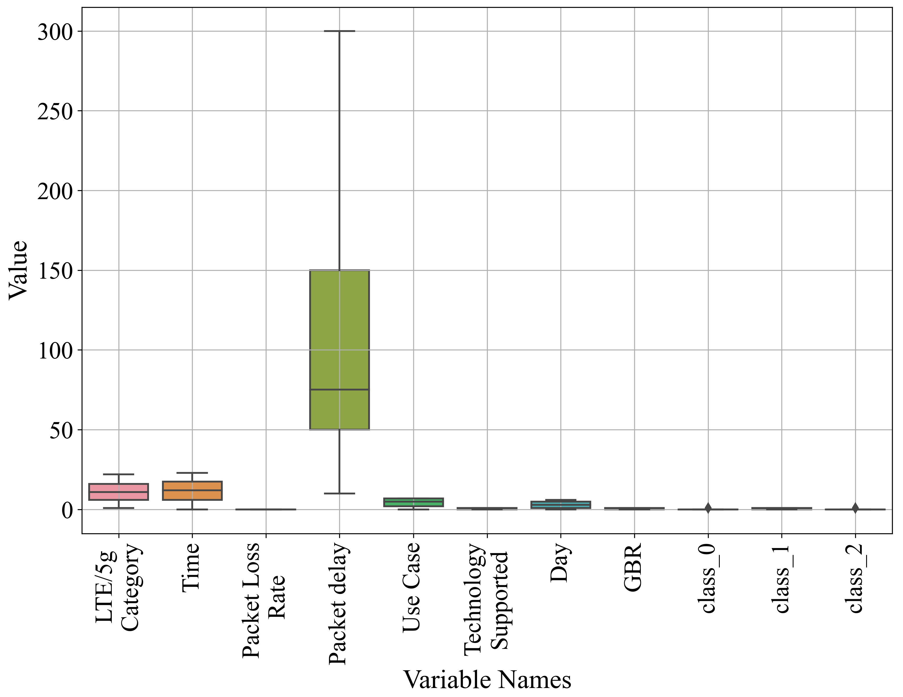
2.2. Dataset Description

As mentioned in the introduction, this paper uses the publicly available dataset from Kaggle (dataset URL available in Dataset Availability Statement). The dataset contains 63,167 samples and 9 variables, with 8 of these variables serving as input features and the remaining variable representing the network slice type, which is the output (target) variable.

The dataset variables are as follows:

• Use Case—types of use cases include Smartphone, Industry 4.0, Smart City and Home, AR/VR/Gaming, IoT Devices, Healthcare, Public Safety, and Smart Transportation.
• LTE/5G Category—it refers to the specific generation or technology level of the network that is being utilized for a particular network slice. The LTE categories are in the 1–16 range, which defines different network capabilities and maximum data rates for LTE devices. Higher categories generally indicate more advanced technologies and higher performance. The 5G categories are in the 1–22 range and are defined for 5G devices and networks. Similar to LTE, the higher categories represent more advanced features and higher performance in terms of data rates, modulation schemes, and other capabilities.
• Technology Supported—this provides information about the underlying communication technologies associated with each network slice.
• Day—the day of the week on which the data were collected.
• Time—the hours of the day at which the data were collected.
• GBR—this stands for Guaranteed Bit Rate, and it is a key parameter in network slicing. The GBR is the minimum data transfer rate that is assured to a network slice for a particular service or application. GBR ensures that a certain amount of network resources, typically bandwidth, is reserved exclusively for the use of specific network slices, even during periods of network congestion. This reservation guarantees a minimum level of performance for applications that require a consistent and reliable data transfer rate.
• Packet Loss Rate—the value of packets that did not reach their destination within the network slice.
• Packet Delay—this refers to the delay experienced by data packets as they traverse the network.
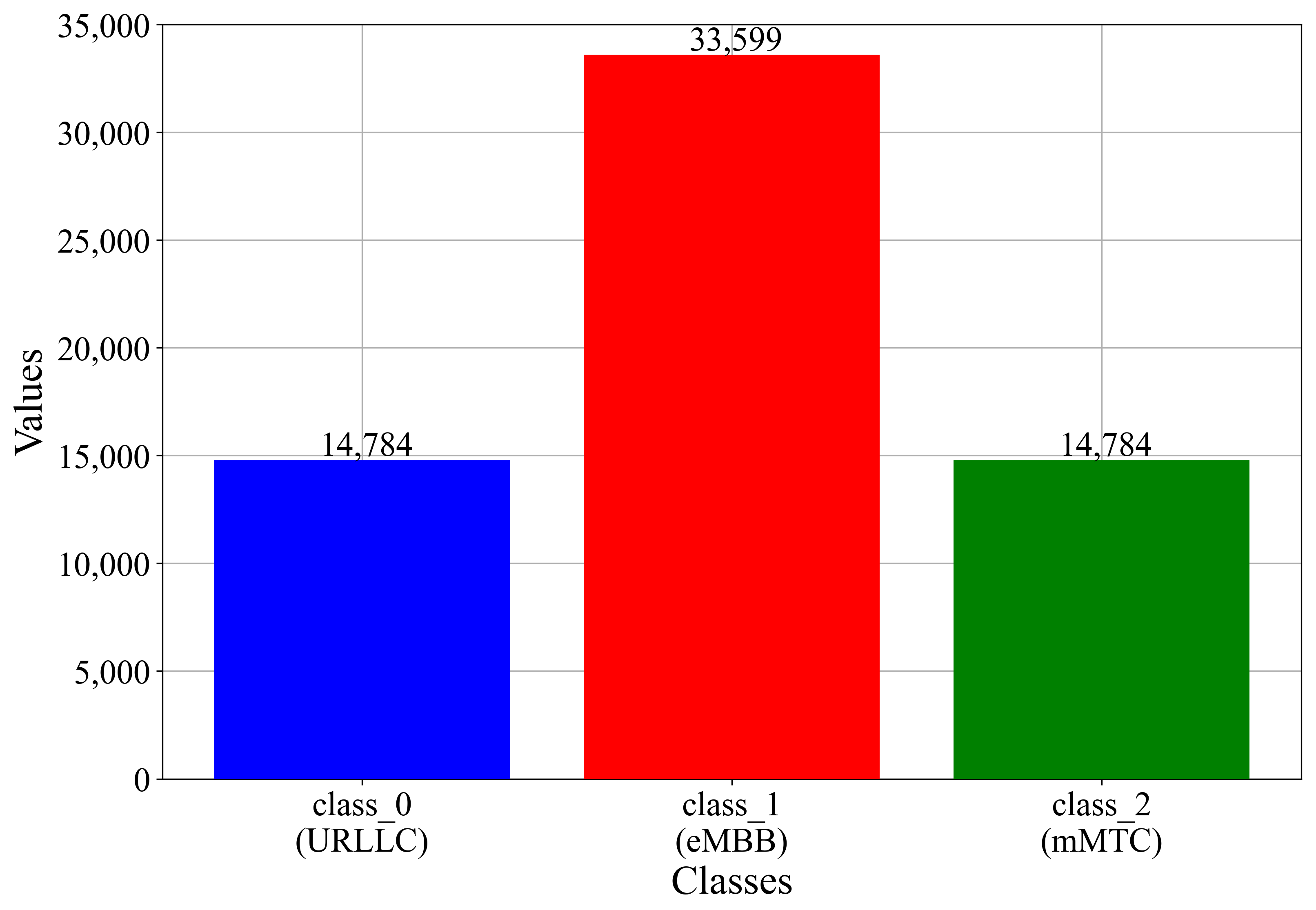
• Slice Type—Mobile Broadband (eMBB), Ultra-Reliable Low-Latency Communication (URLLC), Massive Machine Type Communication (mMTC).

  –

  eMBB—high-bandwidth and high-velocity data transmission; it facilitates activities such as high-definition video streaming, online gaming, and immersive media experiences.

  –

  URLLC—accentuating highly dependable and low-latency connections, it caters to critical applications such as autonomous vehicles, industrial automation, and remote surgery.

  –

  mMTC—concentrating on supporting an extensive multitude of interconnected devices, it enables efficient communication between Internet of Things (IoT) devices, smart cities, and sensor networks.

The initial problem with the dataset is that some variables are not in numeric format, i.e., string format. So, the Label Encoder was applied to these variables. The original values of these variables as well as the corresponding values after application of the Label Encoder are listed in

Table 2. The original values and numeric values assigned after the Label Encoder was applied to categorical variables.

Use Case		Technology Supported		Day		GBR		Slice Type
Original Value	Numeric Value	Original Value	Numeric Value	Original Value	Numeric Value	Original Value	Numeric Value	Original Value	Numeric Value
AR/VR/Gaming	0	IoT (LTE-M, NB-IoT)	0	Monday	0	GBR	0	URLLC	0
Healthcare	1	LTE/5G	1	Tuesday	1	Non-GBR	1	eMBB	1
Industry 4.0	2	—	—	Wednesday	2	—	—	mMTC	2
IoT Devices	3	—	—	Thursday	3	—	—	—	—
Public Safety	4	—	—	Friday	4	—	—	—	—
Smart City and Home	5	—	—	Saturday	5	—	—	—	—
Smart Transportation	6	—	—	Sunday	6	—	—	—	—
Smartphone	7	—	—	—	—	—	—	—	—

.

The dataset contains several categorical variables, all of which were transformed into numerical representations using a Label Encoder. This encoding technique assigns unique integer values to each category within a variable, thereby converting categorical data into a format suitable for machine learning models that require numerical input.

The Use Case variable represents different application domains, including AR/VR/ Gaming, Healthcare, Industry 4.0, IoT Devices, Public Safety, Smart City and Home, Smart Transportation, and Smartphone. Each category was assigned a distinct integer value ranging from 0 (AR/VR/Gaming) to 7 (Smartphone), ensuring a complete numerical representation of all classes.

The Technology Supported variable includes communication technologies such as IoT (LTE-M/NB-IoT) and LTE/5G. These were encoded as 0 and 1, respectively. However, some entries in this column contain missing values, indicating that not all use cases have corresponding technology labels.

The Day variable, representing the days of the week, was also label-encoded. Monday is mapped to 0, and the encoding continues sequentially up to Sunday, which is assigned 6. This ensures numerical compatibility while maintaining the categorical nature of the variable.

The GBR (Guaranteed Bit Rate) variable is categorized into GBR and Non-GBR. Using Label Encoding, GBR is represented by 0 and Non-GBR by 1. Similar to the Technology Supported column, this variable also contains missing values for some rows.

The Slice Type variable denotes the target classes: URLLC, eMBB, and mMTC. These were encoded as 0, 1, and 2, respectively, enabling seamless integration into the machine learning pipeline.

While Label Encoding efficiently transforms categorical data into numeric form, it is important to emphasize that the assigned integers do not imply any ordinal relationship among the categories. For example, the numerical labels AR/VR/Gaming = 0 and Smartphone = 7 do not indicate a hierarchical order. If the learning algorithm is sensitive to such implicit ordering, alternative encoding techniques like one-hot encoding could be more appropriate.

After completing the encoding process, an initial statistical analysis was performed on the transformed dataset. Since the Genetic Programming Symbolic Classifier (GPSC) does not inherently support multiclass classification, the original three-class target variable (Slice Type) was transformed into three binary classification problems using the one-versus-rest (OvR) strategy. For instance, to construct a binary classification dataset for class_0 (URLLC), all instances labeled as URLLC were assigned a target value of 1, while instances labeled as eMBB and mMTC were assigned a value of 0. This process was repeated for each class, resulting in three distinct binary classification datasets.

The results of the initial statistical analysis for all dataset variables, including the three binary target variables, are presented in

Table 3. The results of dataset statistical analysis.

Variable Name	Count	Mean	Std	Min	Max	GPSC Variable Representation	Variable Type
LTE/5G Category	63,167	10.96	6.06	1	22	$X_0$	Input variables
Time		11.50	6.92	0	23	$X_1$
Packet Loss Rate		0.003091	0.004	$1\times {10}^{-6}$	0.01	$X_2$
Packet Delay		114.30	106.32	10	300	$X_3$
Use Case		4.61	2.56	0	7	$X_4$
Technology Supported		0.531907	0.49	0	1	$X_5$
Day		3	2	0	6	$X_6$
GBR		0.55	0.49	0	1	$X_7$
class_0		0.23	0.42	0	1	$y_0$	Output variable
class_1		0.53	0.49	0	1	$y_1$	Output variable
class_2		0.23	0.42	0	1	$y_2$	Output variable

.

As presented in Table 3, the dataset comprises eight input features: LTE/5G Category, Time, Packet Loss Rate, Packet Delay, Use Case, Technology Supported, and Day. Within the Genetic Programming Symbolic Classifier (GPSC) framework, these variables are represented as $X_0$, $X_1$, …, $X_7$, respectively. Based on the count values, there are no missing entries among the dataset variables.

Most input variables display a relatively narrow spread between their minimum and maximum values, suggesting low variance. However, the Packet Delay variable stands out with a wide range—from 0 to 300—which could indicate the presence of outliers or a heavy-tailed distribution. This characteristic may require additional preprocessing or closer examination to ensure robust model performance.

The dataset also includes three binary target variables—class_0, class_1, and class_2—each corresponding to a one-versus-rest classification task. All three use the same set of eight input features. The mean and standard deviation values for these class variables reveal a clear class imbalance. In a balanced binary classification scenario, the mean would typically hover around 0.5, with a low standard deviation. This observed imbalance may affect classifier performance and highlights the need for applying oversampling techniques to reduce model bias.

To assess relationships among the dataset’s variables, Pearson’s correlation analysis [20] is employed. This technique measures the strength and direction of linear associations between continuous variables, producing correlation coefficients ranging from −1 to 1. A coefficient of 1 implies a perfect positive linear relationship, −1 indicates a perfect negative linear relationship, and 0 suggests no linear correlation.

A heatmap visualization of the correlation matrix offers a clear and intuitive overview of these relationships. It allows for quick identification of strong correlations and potential multicollinearity among variables. The color gradient enhances interpretability, making it easier to detect patterns, dependencies, and anomalies that may influence model development or require further analysis. The result of Pearson’s correlation analysis is shown in Figure 2 in the form of a heatmap.

As illustrated in Figure 2, the variables Packet Loss Rate, Packet Delay, Use Case, Technology Supported, and GBR demonstrate varying degrees of correlation with the binary output variables class_0, class_1, and class_2. Specifically, for class_0, the variables Packet Loss Rate, Packet Delay, Use Case, and Technology Supported exhibit negative correlations, while GBR shows a positive correlation. In contrast, for class_1, Packet Loss Rate and GBR are negatively correlated, whereas Packet Delay, Use Case, and Technology Supported display positive correlations. Of particular note is the Technology Supported variable, which demonstrates a perfect positive correlation (1.0) with class_1, potentially indicating a strong deterministic relationship or even a case of data leakage that warrants further scrutiny.

Regarding class_2, the variables Use Case, Technology Supported, and GBR show negative correlations, while Packet Loss Rate and Packet Delay are positively correlated. It is worth emphasizing that none of the correlation coefficients—whether positive or negative—exceed an absolute value of 0.59, suggesting at most moderate relationships between the input features and the target classes.

Additionally, the variables LTE/5G Category, Time, and Day exhibit correlation values close to zero with all three class variables, indicating minimal or no linear association with the target outputs.

Inter-variable correlations are also visible in the heatmap, particularly among Packet Loss Rate, Packet Delay, Use Case, and Technology Supported. These correlations range from −0.17 to 0.41, reflecting weak to moderate dependencies between these features.

Outlier detection is a crucial component of data preprocessing, as outliers—defined as extreme observations that deviate significantly from the overall distribution—can adversely affect statistical summaries and model performance [21]. Outliers may arise from measurement errors, data recording issues, or genuine rare events. Determining their origin is essential to making informed preprocessing decisions, such as removal, transformation, or special treatment.

A boxplot is a valuable visualization tool for identifying outliers. It depicts the central tendency, spread, and potential anomalies within a variable’s distribution. The boxplot highlights the interquartile range (IQR), which contains the middle 50% of values, while whiskers extend to 1.5 times the IQR. Data points lying beyond these whiskers are considered potential outliers. This visualization offers a concise summary of the data distribution and helps analysts quickly detect values that deviate from expected patterns, facilitating further examination or correction before model training. The boxplot showing the range of values of all dataset variables is shown in Figure 3.

As illustrated by the boxplot in Figure 3, none of the input variables exhibit outliers. Most features have values ranging between 0 and a maximum of 23, with the exception of the Packet Delay variable, which spans a broader range from 10 to 300. This extended range may reflect genuine variability in the data rather than the presence of anomalous values, as the distribution appears consistent and within expected bounds.

Following the confirmation that the dataset is free of outliers, the next logical step is to examine the distribution of class labels within the initial dataset. The bar plot presented in Figure 4 displays the number of samples associated with each class, offering a visual representation of potential class imbalance issues that may need to be addressed through oversampling techniques.

As illustrated in Figure 4, the dataset exhibits an imbalanced distribution among the classes: both class_0 and class_2 contain an equal number of samples, whereas class_1 has approximately 2.27 times more instances than either of the other two. Given the multiclass nature of the classification task, two distinct strategies can be employed when training the Genetic Programming Symbolic Classifier (GPSC):

• The first strategy maintains the original target variable but applies oversampling techniques to generate balanced versions of the dataset. The one-versus-rest (OvR) approach is then used during training, allowing the GPSC to treat each class individually.
• The second strategy converts the multiclass target into three separate binary classification problems. For instance, when training for class_0, all its instances are labeled as 1, while instances of *class_1* and class_2 are labeled as 0. This conversion is repeated for each class, resulting in three dedicated binary datasets—each focusing on one class versus the rest.

A summary of the sample distribution per class under each approach is provided in

Table 4. The binary datasets for class_0, 1, and 2—the number of samples that belong/do not belong to specific class in the binary classification dataset.

Dataset Name	Samples Belong to the Class	Samples Do Not Belong to the Class
Initial dataset class_0	14,784	48,383
Initial dataset class_1	33,599	29,568
Initial dataset class_2	14,784	48,383

.

2.3. Oversampling Techniques

To achieve a synthetic balance between class samples, several oversampling techniques were considered, including KMeansSMOTE, SMOTE, and Random Oversampling. Initially, other techniques such as ADASYN, BorderlineSMOTE, and SVMSMOTE were also considered. However, these methods did not lead to the creation of balanced dataset variations. Oversampling techniques were preferred over undersampling methods, as they can quickly achieve a balanced dataset and do not require fine-tuning, unlike undersampling techniques.

2.3.1. KMeansSMOTE

KMeansSMOTE [22] is an extension of the Synthetic Minority Oversampling Technique (SMOTE), which integrates the KMeans clustering algorithm to improve upon traditional SMOTE, particularly in cases with overlapping classes. The process begins with applying KMeans clustering to identify clusters within the feature space. Synthetic instances are then generated specifically within these clusters, helping to avoid the issues faced by traditional SMOTE when class distributions are not clearly separable. This approach ensures that synthetic instances are created within local regions of the feature space, where the minority class is concentrated. The advantages of KMeansSMOTE are as follows:

• KMeansSMOTE addresses class overlap and is useful for noisy datasets.
• It generates synthetic instances within clusters, contributing to better generalization.
• It enhances model robustness in complex data distributions, where traditional SMOTE might fail.

The disadvantages of KMeansSMOTE are as follows:

• The method requires tuning additional parameters, such as the number of clusters in the KMeans algorithm. Poor selection of the number of clusters can impact the quality of the synthetic instances.
• The computational complexity is higher than that of traditional SMOTE due to the clustering step, which could be a challenge with large datasets or in resource-constrained environments.

2.3.2. SMOTE

The Synthetic Minority Oversampling Technique (SMOTE) [23] is a widely adopted method for addressing class imbalance in classification tasks. It operates by generating synthetic samples for the minority class to balance the dataset. Specifically, SMOTE creates new instances by interpolating between a randomly selected minority class sample and one of its k-nearest neighbors. These synthetic points are generated along the line segments joining the original sample and its neighbors, effectively enriching the minority class distribution.

Key advantages of SMOTE include the following:

• It effectively balances the dataset by increasing the representation of the minority class, which can lead to improved classification performance.
• SMOTE mitigates model bias toward the majority class and reduces the risk of overfitting by avoiding simple duplication of minority class samples.
• The method promotes better generalization by introducing variability into the training data through synthetic sampling.

However, SMOTE also presents some limitations:

• It may be less effective in datasets with high noise levels or significant class overlap, where generated samples might introduce ambiguity and degrade model performance.
• The effectiveness of SMOTE is highly dependent on the choice of the k parameter (number of nearest neighbors). An inappropriate k value may produce synthetic samples that do not accurately reflect the underlying data distribution, necessitating careful parameter tuning.

2.3.3. Random Oversampling

Random Oversampling [24] is a simple technique for addressing class imbalance by duplicating instances from the minority class until a more balanced dataset is achieved. This oversampling is performed randomly without considering the specific characteristics of the instances. The advantages of Random Oversampling are as follows:

• Simplicity: Random Oversampling is easy to implement and requires minimal parameter tuning.
• Computational Efficiency: it is a straightforward and computationally efficient technique, especially when the class imbalance is not extreme.
• Prevention of Model Bias: by duplicating instances of the minority class, it helps prevent bias towards the majority class, ensuring a more equitable representation.

The disadvantages of Random Oversampling are as follows:

• Risk of Overfitting: Duplicating instances without regard for their characteristics can lead to overfitting the minority class. The model might learn redundant patterns that do not generalize well to unseen data.
• Lack of Diversity: Since only existing instances are duplicated, this method does not introduce any diversity into the dataset. This may limit the model’s ability to generalize to new data, especially in cases of severe imbalance.

2.3.4. Datasets Obtained from Application of Oversampling Techniques

After the application of all previously described oversampling techniques, the balanced dataset variations for each class were achieved. In

Table 5. Results of application of different oversampling techniques and comparison to initial imbalanced dataset.

Dataset Name	Belong to Class (Label 1)	Do Not Belong to Class (Label 0)	Total Samples Number
Initial dataset Class 0	14,784	48,383	63,167
Initial dataset Class 1	29,568	33,599	63,167
Initial dataset Class 2	14,784	48,383	63,167
KMeansSMOTE Class 0	48,383	48,383	96,766
Random Oversampling Class 0	48,383	48,383	96,766
SMOTE Class 0	48,383	48,383	96,766
KMeansSMOTE Class 1	33,599	33,601	67,200
Random Oversampling Class 1	33,599	33,599	67,198
SMOTE Class 1	33,599	33,599	67,198
KMeansSMOTE Class 2	48,385	48,383	96,768
Random Oversampling Class 2	48,383	48,383	96,766
SMOTE Class 2	48,383	48,383	96,766

, the number of samples for each class in each dataset variation is listed.

As shown in Table 5, most oversampling techniques successfully balanced the original datasets, resulting in corresponding balanced dataset variations. However, in a few cases, the class distributions remained slightly imbalanced even after applying oversampling. For instance, in the KMeansSMOTE Class 1 dataset, the number of samples belonging to the class is 33,599, while the number of samples not belonging to the class is 33,601. Originally, Class 1 had 29,568 positive and 33,599 negative samples. Although the minority class was correctly oversampled, two additional samples were also added to the majority class, resulting in a marginal discrepancy.

A similar situation occurred with the KMeansSMOTE Class 2 dataset, where the oversampling process resulted in the minority class (belonging to Class 2) having slightly more samples than the majority class (not belonging to Class 2). In both cases, the discrepancy is minimal (only 2 samples), which is negligible compared to the initial class imbalance.

After generating the balanced dataset variations, the Genetic Programming Symbolic Classifier (GPSC) with the Repeated Holdout Validation Strategy (RHVS) was applied to each to obtain symbolic expressions (SEs) with high classification accuracy.

2.4. Genetic Programming Symbolic Classifier

The Genetic Programming Symbolic Classifier [25] begins its execution with the creation of an initial (naive) set of population members (symbolic expressions) that are unfit for particular tasks. With the application of genetic operation for a predefined number of generations, the population members evolve, and eventually, they are fit for particular tasks. The output of each GPSC execution is one symbolic expression that has high classification accuracy.

The GPSC is an evolutionary algorithm; however, for proper execution, it requires a dataset with defined input and output, just like the majority of supervised machine learning algorithms. The problem with the GPSC in obtaining the symbolic expression is to obtain the symbolic expression with high classification accuracy. To accomplish this, it is necessary to find optimal combinations of GPSC hyperparameters. So, to find the optimal combination of GPSC hyperparameters, the random hyperparameter values search method is developed and applied. This method randomly selects the hyperparameter value from a predefined range each time it is called, which is before each GPSC execution. To develop the RHVS method, several steps are required:

• Define the initial boundary values of each hyperparameter;
• Test each GPSC hyperparameter boundary value to see if the GPSC will successfully execute;
• If needed, adjust the boundaries of each GPSC hyperparameter before applying it in research.

The following GPSC hyperparameters were utilized within the RHVS method:

• PopSize—this defines the size of the population that will be evolved by the GPSC algorithm.
• GenNum—this specifies the number of generations used to evolve the population. This serves as one of the termination criteria, meaning that the GPSC will stop once the specified number of generations is reached.
• InitTreeDepth—this sets the depth range for the initial population trees. In the GPSC, each symbolic expression is represented as a tree, with the root node being a mathematical function. The tree is constructed from the root to the deepest leaf node, which can contain mathematical functions, input variables, or constants. The initial trees are generated using the ramped half-and-half method: half of the population is created using the full method (trees of maximum depth), while the other half uses the grow method (trees of variable shape). The “ramped” aspect refers to selecting tree depths from a defined range. For example, a range of (5, 18) creates initial trees with depths between 5 and 18.
• TournamentSize—this determines the number of population members randomly selected to participate in tournament selection. The member with the lowest fitness value generally wins, but the tree length (i.e., complexity) is also considered through the parsimony pressure method (controlled by ParsimonyCoeff). This helps avoid selecting overly complex solutions. Genetic operations such as crossover or mutation are then applied to the tournament winners.
• Crossover—this specifies the probability of applying the crossover operation. This operation requires two selected individuals (tournament winners). A random subtree is selected from each, and the subtree from the second individual replaces the one in the first to generate a new individual for the next generation.
• SubtreeMute—this defines the probability of performing subtree mutation. This operation selects a random subtree in a single individual and replaces it with a newly generated subtree using available functions, variables, and constants.
• PointMute—this specifies the probability of applying point mutation. This operation randomly selects nodes within an individual and modifies them: constants are replaced with new constants, variables with other variables, and functions with others requiring the same number of input arguments.
• HoistMute—this sets the probability of hoist mutation. A random subtree is selected from the individual, and a random node within that subtree replaces the entire subtree, creating a new individual for the next generation.
• ConstRange—this defines the range of constant values used when constructing initial trees and during mutation operations.
• StoppingCrit—this sets a minimum fitness threshold as a termination criterion. If a population member’s fitness drops below this predefined value, the GPSC execution is terminated early. The fitness function in the GPSC is computed as follows:
  • The training set samples (values of input variables) are used to compute the output of the population member.
  • This output is used in the Sigmoid function as the input to compute the output i.e., to determine the class (0 or 1). The Sigmoid function can be written as:

    $$S\left(x\right)={\displaystyle \frac{1}{1+e^{-x}}}$$

    (1)

    where x is the output generated by the population member.
  • The output of the Sigmoid function is used as the input alongside the real output from the dataset to compute the LogLoss value. The LogLoss formula can be written as:

    $$L\left(x\right)=-{\displaystyle \frac{1}{N}}\sum _{i=1}^N(y_i·log\left(p\left(y_i\right)\right)+(1-y_i)·log(1-p\left(y_i\right)))$$

    (2)

    where N is the number of dataset samples, y is the true label (0 or 1), and p is the predicted probability that the sample belongs to Class 1.
• MinSize—this indicates the minimum fraction of the training set to be used in evaluating individuals. A value slightly less than 1 enables the estimation of out-of-bag (OOB) fitness. OOB samples are those excluded from an individual’s training subset and are used to estimate generalization performance without requiring a separate validation set.
• ParsimonyCoeff—the coefficient used in the parsimony pressure method to prevent bloat, a phenomenon where individuals grow excessively large without fitness improvement. Large individuals have their fitness penalized proportionally to their size, making them less likely to win tournament selection. This prevents prolonged execution times and memory exhaustion errors. The adjusted fitness f is computed as:

  $$f^{\prime }=f+\lambda L$$

  (3)

  where f is the original fitness, L is the size (length) of the individual, and $\lambda$ is the parsimony coefficient.

It is important to note that the sum of the probabilities for all genetic operations should be approximately 1. If this condition is not met, some tournament selection winners might be passed into the next generation without modification—i.e., no genetic operations would be applied to certain individuals.

The set of mathematical functions used in this research includes +, −, ×, ÷, √, $\sqrt[3]{}$, log, ${log}_2$, ${log}_{10}$, ‖, sin, cos, and tan. However, certain functions—specifically ÷, √, log, ${log}_2$, and ${log}_{10}$—required modifications to prevent errors in GPSC execution, such as the generation of nan (not a number) or imaginary values. The modifications made to these functions are outlined in the Appendix A.

The boundaries for each GPSC hyperparameter are listed in

Table 6. The boundaries of GPSC hyperparameters used in the RHVS method.

Hyperparameter Name	Lower Boundary	Upper Boundary
PopSize	1000	2000
GenNum	200	300
InitTreeDepth	3	18
TournamentSize	100	500
Crossover	0.001	1
SubtreeMute	0.001	1
PointMute	0.001	1
HoistMute	0.001	1
ConstRange	−1,000,000	1,000,000
StoppingCrit	$1\times {10}^{-6}$	$1\times {10}^{-3}$
MinSize	0.99	1
ParsimonyCoeff	$1\times {10}^{-7}$	$1\times {10}^{-6}$

.

2.5. Evaluation Metrics

To assess the symbolic expressions generated after each GPSC execution, several evaluation metrics were employed, including accuracy, area under the receiver operating characteristic curve (AUC), precision, recall, F1-score, and the confusion matrix. However, the confusion matrix was primarily used to evaluate the final set of symbolic expressions.

The accuracy score, as defined by [26], quantifies the overall correctness of a classification model. It is calculated as the ratio of correctly predicted instances to the total number of predictions. The formula for calculating accuracy is as follows:

$$ACC={\displaystyle \frac{\mathrm{Number}\mathrm{of}\mathrm{Correct}\mathrm{Predictions}}{\mathrm{Total}\mathrm{number}\mathrm{of}\mathrm{predictions}}}={\displaystyle \frac{TP+TN}{TP+TN+FP+FN}},$$

(4)

where $TP$, $TN$, $FP$, and $FN$ represent true positives, true negatives, false positives, and false negatives, respectively. True positives ($TP$) refer to dataset samples that are correctly classified as positive. True negatives ($TN$) are dataset samples correctly identified as negative. False positives ($FP$) are instances incorrectly predicted as positive, while false negatives ($FN$) are those incorrectly predicted as negative.

The area under the receiver operating characteristic curve (AUC), as defined in [26], serves as a performance measure for classification problems across various threshold settings. The AUC is the area beneath the ROC curve, which plots the true positive rate against the false positive rate.

As per [26], precision is a metric that quantifies the accuracy of positive predictions made by the model. It is the ratio of true positive predictions to the total number of positive predictions. Precision is calculated using the following expression:

$$Precision={\displaystyle \frac{TP}{TP+FP}}$$

(5)

where $TP$ and $FP$ represent true positives and false positives, respectively.

The recall, as described in [26], is a measure of the model’s ability to identify all relevant instances. It is defined as the ratio of true positive predictions to the total number of actual positive instances, which includes both true positives and false negatives. The recall is calculated using the following expression:

$$Recall={\displaystyle \frac{TP}{TP+FN}}$$

(6)

where $FN$ represents the false negatives.

The F1-score [26] is the harmonic mean of precision and recall, providing a balance between the two metrics while taking both false positives (FP) and false negatives (FN) into account. The formula for calculating the F1 score is given by:

$$F1\text{-}score={\displaystyle \frac{2·Precision·Recall}{Precision+Recall}}$$

(7)

The F1-score is a useful metric when there is an uneven class distribution, and both false positives (FP) and false negatives (FN) need to be minimized.

The confusion matrix is a table that provides a summary of the classification model’s performance, showing counts of true positives (TP), true negatives (TN), false positives (FP), and false negatives (FN).

According to [27], the confusion matrix can be defined as a table that summarizes the predicted and actual classes, displaying the counts of TP, TN, FP, and FN.

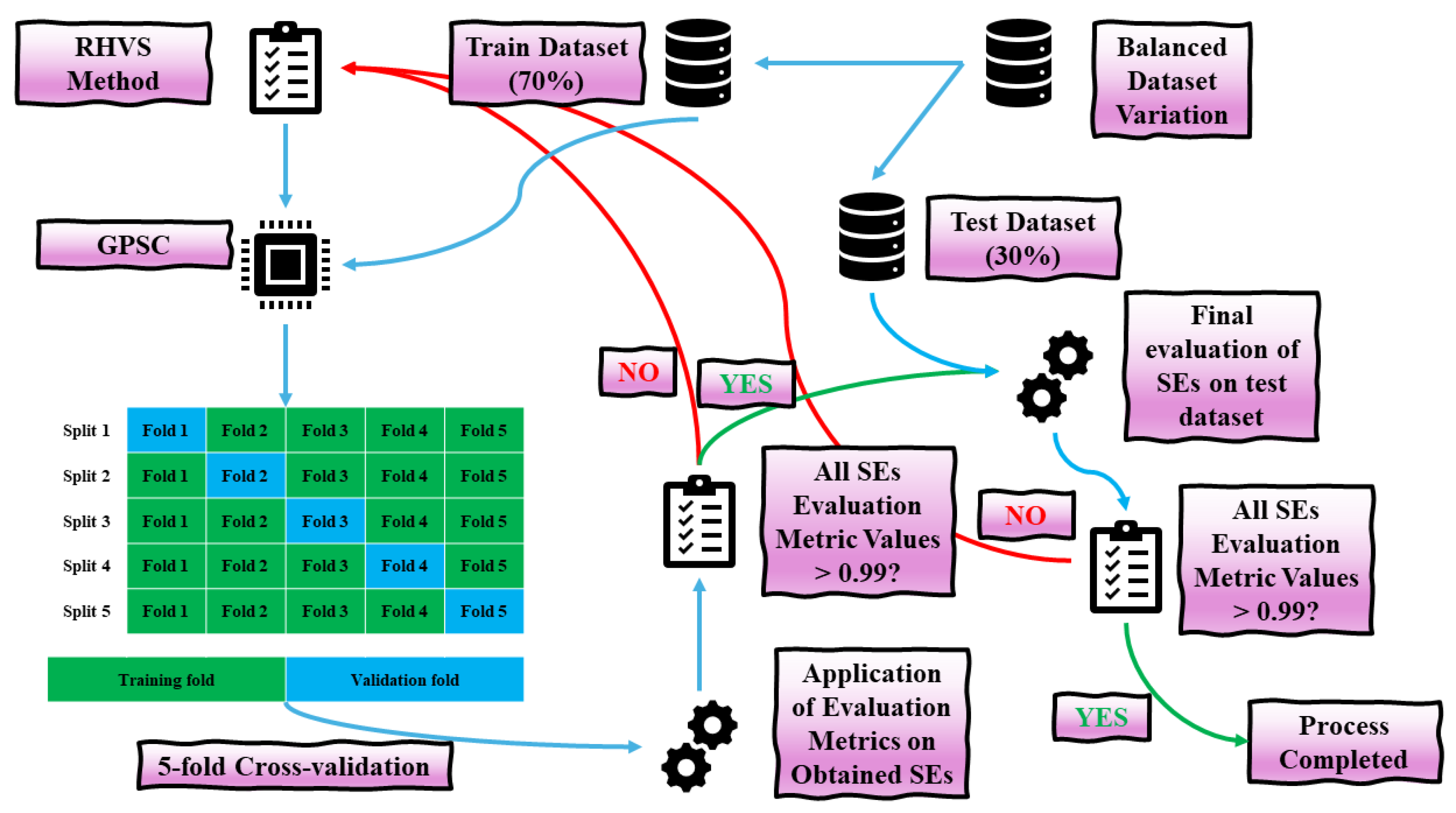
2.6. Training/Testing Procedure

The graphical representation of the training procedure used in this paper is shown in Figure 5.

As illustrated in Figure 5, the training and testing procedure follows these steps:

• Each balanced dataset variation, on which the GPSC was applied, was split into training and testing subsets with a 70:30 ratio, where 70% of the data were used for training and the remaining 30% were reserved for testing.
• After the initial dataset split, the RHVS method was invoked, randomly selecting GPSC hyperparameter values from predefined boundaries. These hyperparameters were then used in the GPSC, which was trained using 5-fold cross-validation.
• Following 5-fold cross-validation, five symbolic expressions were obtained as the GPSC was trained on each fold. For these five symbolic expressions, the mean evaluation metric values (ACC, AUC, precision, recall, and F1-score) were calculated, along with their standard deviation ($\sigma$).
• If the mean evaluation metrics exceeded 0.99, the process moved to the testing phase, where the symbolic expressions were tested on the remaining 30% of the dataset. If the mean evaluation metrics were below 0.99, the process was restarted with a new random selection of GPSC hyperparameters using the RHVS method.
• During the testing phase, the testing dataset was applied to the five symbolic expressions, and the mean evaluation metrics were recalculated from both the training and testing phases. If all evaluation metrics exceeded 0.99, the process was completed. If not, the process was repeated, starting with a new random selection of hyperparameters.

3. Results

Initially, the results from the balanced dataset variations will be presented, highlighting the optimal combination of GPSC hyperparameter values that yielded the symbolic expression with the highest classification performance. Subsequently, the top-performing symbolic expressions will be combined and evaluated on the original imbalanced dataset, with adjustments made to the minimum number of correct predictions considered for each sample.

3.1. The Results Obtained on the Balanced Dataset Variations

As outlined in the Section 2, the initial imbalanced dataset was effectively balanced using the KMeansSMOTE, SMOTE, and Random Oversampling techniques, resulting in three balanced dataset variations for each class. The optimal combination of GPSC hyperparameters, which produced symbolic expressions with high classification performance for each balanced dataset variation, is presented in

Table 7. The optimal combination of GPSC hyperparameter values, with which the best sets of symbolic expressions were obtained on each balanced dataset variation.

Dataset	PopSize, GenNum, TournamentSize, InitTreeDepth, Crossover, SubtreeMute, PointMute, HoistMute, StoppingCrit, MaxSamples, ConstRange, ParsimonyCoeff
KMeansSMOTE Class 0	1635, 250, 481, (4, 12), 0.0087, 0.975, 0.011, 0.0036, 0.000925, 0.997, (−301,700.69, 942,674.18), $5.88\times {10}^{-7}$
Random Oversampling Class 0	1661, 209, 141, (7, 17), 0.003, 0.95, 0.021, 0.019, 0.000129, 0.995, (−596,786.6, 272,352.52), $9.23\times {10}^{-7}$
SMOTE Class 0	1801, 286, 429, (6, 12), 0.039, 0.956, 0.0019, 0.0027, 0.00032, 0.99, (−178,629.2, 152,684.75), $1.51\times {10}^{-7}$
KMeansSMOTE Class 1	1009, 253, 168, (7, 13), 0.012, 0.954, 0.014, 0.018, $7.8\times {10}^{-5}$, 0.992, (−961,606.57, 916,549.35), $9.82\times {10}^{-7}$
Random Oversampling Class 1	1232, 226, 435, (7, 12), 0.021, 0.954, 0.019, 0.0041, 0.000441, 0.995, (−191,244.26, 675,108.15), $5.13\times {10}^{-7}$
SMOTE Class 1	1570, 228, 249, (3, 12), 0.01, 0.961, 0.013, 0.0148, $1.3\times {10}^{-5}$, 0.997, (−448,676.52, 295,584.56), $2.06\times {10}^{-7}$
KMeansSMOTE Class 2	1145, 202, 397, (4, 14), 0.0017, 0.959, 0.033, 0.0044, 0.000398, 0.993, (−495,217.82, 691,481.82), $3.91\times {10}^{-7}$
Random Oversampling Class 2	1786, 267, 250, (7, 12), 0.0094, 0.95, 0.0071, 0.03, $2.9\times {10}^{-5}$, 0.99, (−987,687.37, 676,238.71), $6.31\times {10}^{-7}$
SMOTE Class 2	1504, 262, 345, (6, 14), 0.001, 0.96, 0.034, 0.0028, 0.00054, 0.997, (−200,908.45, 851,092.06), $2.74\times {10}^{-7}$

.

In most GPSC applications conducted on the balanced dataset variations, the population size (PopSize) exceeded 1500. Only three cases had a PopSize below this threshold—namely, KMeansSMOTE Class 1, Random Oversampling Class 1, and KMeansSMOTE Class 2, as shown in Table 7.

The lowest number of generations (GenNum) was 202 for the KMeansSMOTE Class 2 dataset, while the highest value was 286 for the SMOTE Class 0 dataset. For the majority of cases, GenNum values ranged between 209 and 267. However, in all GPSC experiments, GenNum was never reached as a termination criterion. In most runs, the fitness value of at least one population member fell below the predefined stopping criterion after approximately 50 generations, prompting early termination.

The TournamentSize hyperparameter was highest (481) for the KMeansSMOTE Class 0 dataset—close to the upper boundary defined by the RHVS method—and lowest for the Random Oversampling Class 0 dataset. The InitTreeDepth range was widest for KMeansSMOTE Class 2 and Random Oversampling Class 0 ((4, 14) and (7, 17), respectively), while the narrowest range (7, 12) was used for Random Oversampling Class 2.

Across all experiments, the dominant genetic operation was subtree mutation, with a consistent rate between 0.95 and 0.975.

The lowest stopping criterion (StoppingCrit) value of $1.3\times {10}^{-5}$ was used for the SMOTE Class 1 dataset, while the highest value (0.000925) was used for KMeansSMOTE Class 0. This criterion served as the primary termination condition for the GPSC, as none of the experiments reached the GenNum limit.

The minimum size of training samples (MinSize) was consistently set to around 0.99 (99%) across all GPSC runs.

Although the parsimony coefficient was set to an extremely low value (${10}^{-7}$), the bloat phenomenon was not observed. This is evident from the high classification performance achieved (see Figure 6) and from

Table 8. The length and depth of the best sets of SEs obtained on each balanced dataset variation.

Dataset		SE1	SE2	SE3	SE4	SE5	Average
KMeansSMOTE Class 0	Depth	4	12	21	5	8	10
	Length	8	57	54	21	25	33
Random Oversampling Class 0	Depth	13	13	10	10	6	10.4
	Length	26	179	26	71	11	62.2
SMOTE Class 0	Depth	3	3	11	10	7	6.8
	Length	8	5	32	41	55	28.2
KMeansSMOTE Class 1	Dept	12	9	3	13	5	8.4
	Length	60	24	8	29	13	26.8
Random Oversampling Class 1	Dept	17	2	14	22	7	12.4
	Length	142	7	31	90	54	64.8
SMOTE Class 1	Dept	8	2	5	5	4	4.8
	Length	11	6	12	13	20	12.4
KMeansSMOTE Class 2	Dept	26	12	15	13	9	15
	Length	78	77	80	79	42	71.2
Random Oversampling Class 2	Dept	5	16	9	9	26	13
	Length	11	81	64	45	113	62.8
SMOTE Class 2	Dept	10	9	11	11	15	11.2
	Length	44	40	56	25	65	46

, where the depth and length of the best-obtained symbolic expressions (SEs) are listed—none of which exceeds 200 elements in length.

Using this combination of hyperparameters on the corresponding dataset variation, the symbolic expressions were obtained with high classification performance. An example of one symbolic expression for detecting Class 0 can be written as:

$$y_0=25.5313sin(log\left(X_3\right))$$

(8)

For detecting Class 1, an example of symbolic expression can be written as:

$$y_1=-142488-X_0+644416X_5,$$

(9)

For detecting Class 2, an example of symbolic expression can be written as:

$$y_2=577985\left(-X_5+0.43log(0.43log(X_3-X_7))\right)$$

(10)

From previous examples of symbolic expressions, it can be noticed that not all input variables are required to compute the output. However, to use all of the obtained symbolic expressions, all input variables are required. The procedure of downloading and using obtained symbolic expressions from this investigation is described in Appendix B.

The size of obtained symbolic expressions can be measured in the form of depth and length. Since the symbolic expression can be represented in tree form, the depth is measured from the root node up to the deepest leaf of the tree. The symbolic expression length is measured as the number of elements (mathematical functions, constants, and input variables) in symbolic expression. In Table 8, the depth and length for each of the best symbolic expressions for each class are shown.

As seen in Table 8, the lowest average depth is that of SEs obtained on the SMOTE Class 1 dataset. The highest average depth is that of SEs obtained on KMeansSMOTE Class 2. The lowest average length is that of SEs obtained on SMOTE Class 1, while the highest average length is that of SEs obtained on the KMeansSMOTE Class 2 dataset. When SEs for each class are examined and obtained on different dataset variations, it can be noticed that for class_0 the lowest average depth is that of SEs obtained on the SMOTE Class 0 dataset, while the highest average depth is that of SEs obtained on the Random Oversampling Class 0 dataset. The lowest and highest average lengths are also those of SEs obtained on previously mentioned dataset variations. In the case of SEs for class_1, the lowest average depth and length are those of SEs obtained on the SMOTE Class 1 dataset, while the largest average depth and length are those of SEs obtained on the Random Oversampling Class 1 dataset. In the case of class_2, the lowest average depth and length are those of SEs obtained on the SMOTE Class 2 dataset, while the highest average length and depth are those of SEs obtained on the KMeansSMOTE Class 2 dataset.

It is interesting to notice that SEs with the same depth value have different length values. For example, in the case of SEs 1 and 2 obtained on the Random Oversampling Class 0 dataset, they both have a depth value of 13. However, the length value of SE 1 is 26, while the length value of SE 2 is 179. This means that SE 2 has almost 7 times more node elements (input variables, constants, and mathematical functions) than SE 1. Another example is SEs 1 and 2 obtained on the SMOTE Class 0 dataset that have the same depth (3), while the lengths are 8 and 5, respectively. Other examples are SEs 3 and 4 obtained on the Random Oversampling Class 2 dataset and SMOTE Class 2 dataset. So, the same depth of SEs in tree form can have different lengths in normal form (equation), i.e., different numbers of elements.

The evaluation metric values of all the best symbolic expressions are shown in Figure 6.

As seen in Figure 6, all the best SEs achieved extremely high classification performance (1.0) on all balanced dataset variations. The mean values of all evaluation metrics used in this research are equal to 1, and the value of the standard deviation for all SEs is equal to 0.0.

3.2. Evaluation of All Symbolic Expressions on Initial Dataset

The optimal sets of symbolic expressions for Classes 0, 1, and 2, derived from the balanced dataset variations, were tested on the original imbalanced dataset obtained after the initial data preprocessing. The classification performance of these best symbolic expressions for each class is displayed in Figure 7 and summarized in the form of confusion matrices in

Table 9. The classification performance of the combination of the best SEs applied on the imbalanced dataset.

Evaluation Metric	Initial Dataset Class_0	Initial Dataset Class_1	Initial Dataset Class_2
$ACC$	1.0	1.0	1.0
$AUC$	1.0	1.0	1.0
$Precision$	1.0	1.0	1.0
$Recall$	1.0	1.0	1.0
$F1$-$Score$	1.0	1.0	1.0

.

As seen in Figure 7 and Table 9, the classification performance of all the best SEs is extremely high. The SEs can perfectly classify all the dataset samples.

4. Discussion

As detailed in the Section 2, this study utilizes a publicly available dataset from Kaggle, which includes eight input variables and one output variable, forming a multiclass classification problem. For binary classification purposes, the original target variable was divided into three binary cases: the first output variable (class_0) represents URLLC, the second (class_1) corresponds to eMBB, and the third (class_2) pertains to mMTC.

An initial challenge with the dataset was that four input variables—Use Case ($X_4$), Technology Supported ($X_5$), Day ($X_6$), and GBR ($X_7$)—were in string format. To address this, Label Encoding was applied to convert these categorical features into numerical values, as presented in Table 2.

The distribution of the output classes showed imbalances, which required the application of oversampling techniques to create a more balanced dataset for training.

Regarding feature correlations, as depicted in Figure 2, the variables Packet Loss Rate, Packet Delay, Use Case, and Technology Supported exhibit moderate correlations with the target classes, with correlation coefficients ranging from −0.59 to 0.59. In contrast, the variables LTE/5G Category, Time, and Day show no correlation with the output variables, having correlation values of zero.

No outliers were detected in the dataset. Most input variables have values ranging from 0 to 23, except for Packet Delay, which ranges from 0 to 300. Due to the limited occurrence of large-scale values in only one variable, data preprocessing techniques such as normalization or scaling were not considered necessary.

In this study, oversampling techniques were used to address the initial class imbalance in the datasets. The main reason for selecting oversampling over undersampling methods was their lower need for hyperparameter tuning and faster execution times. While undersampling requires identifying and removing instances—a process that can be computationally expensive—oversampling generates synthetic samples, making it a more efficient approach in many practical scenarios.

Various oversampling techniques were considered, including ADASYN, BorderlineSMOTE, SMOTE, KMeansSMOTE, SVMSMOTE, and Random Oversampling. However, only KMeansSMOTE, SMOTE, and Random Oversampling were successfully implemented. These three methods resulted in nine balanced dataset variations, derived from the original three imbalanced datasets (i.e., using class_0, class_1, and class_2 as target variables).

The effectiveness of these techniques in balancing the datasets is summarized in Table 5. It is important to note that two variations—KMeansSMOTE Class 1 and KMeansSMOTE Class 2—showed a minor imbalance after oversampling, with only a two-sample difference between the majority and minority classes. However, this discrepancy is insignificant compared to the substantial class imbalance in the original datasets.

The GPSC training process was conducted on all nine balanced dataset variations, with the Randomized Hyperparameter Value Search (RHVS) method employed for hyperparameter optimization. Training was carried out using 5-fold cross-validation (5FCV), where the dataset was divided into five folds and a symbolic expression (SE) was generated for each fold using the GPSC.

As a result, five SEs were produced for each balanced dataset variation. Thus, for each target class—class_0, class_1, and class_2—a total of 15 SEs were generated (i.e., 5 SEs × 3 balanced variations per class). In total, across all nine balanced dataset variations, the GPSC training process resulted in 45 high-performing SEs.

To determine the best set of SEs for each dataset variation, the optimal combination of GPSC hyperparameters was selected using the RHVS method. The term “optimal” refers to the set of GPSC hyperparameter values that resulted in the highest classification performance, specifically the highest values for ACC, AUC, precision, recall, and F1-score.

As presented in Table 7, the largest population size (PopSize) of 1801 was selected for the SMOTE Class 0 dataset, followed by a PopSize of 1786 for the Random Oversampling Class 2 dataset. These values are close to the upper boundary of the PopSize range explored in the RHVS method. Larger PopSize values were generally preferred to enhance population diversity, which is essential for effectively exploring the solution space.

Another critical hyperparameter influencing population diversity is the initial tree depth (InitTreeDepth) used in the ramped half-and-half initialization method. The largest InitTreeDepth range, (4, 14), was applied to the KMeansSMOTE Class 2 dataset.

Although the maximum number of generations (GenNum) was defined as one of the termination criteria, alongside the stopping criterion (StoppingCrit), it was never reached during GPSC training. The fitness value of population members typically dropped below the predefined StoppingCrit threshold within the first few dozen generations, rendering the GenNum irrelevant.

Across all GPSC investigations, subtree mutation was the dominant genetic operation, consistently set at or above 0.95. The parsimony coefficient, aimed at controlling expression size and preventing bloat, was set to a very small value (${10}^{-7}$) in all experiments. While such a small value might generally increase the risk of bloat, the early termination triggered by StoppingCrit effectively mitigated this issue. However, closer inspection revealed that certain datasets, such as Random Oversampling Class 0 and Class 1, KMeansSMOTE Class 2, Random Oversampling Class 2, and SMOTE Class 2, did result in larger symbolic expressions (SEs), indicating that the small parsimony coefficient may still have influenced SE complexity in these cases.

Table 8 provides a detailed overview of the best-performing SEs across all dataset variations. The lowest average depth and length were observed in SEs derived from the SMOTE Class 1 dataset, while the highest values were found in SEs from the KMeansSMOTE Class 2 dataset.

Class-specific patterns were also noted:

• For class_0, the lowest average depth and length were observed in the SMOTE Class 0 dataset, while the highest values were seen in the Random Oversampling Class 0 dataset.
• For class_1, SEs from the SMOTE Class 1 dataset exhibited the lowest depth and length, while the highest values came from the Random Oversampling Class 1 dataset.
• For class_2, SEs from the SMOTE Class 2 dataset had the lowest values, and those from KMeansSMOTE Class 2 had the highest.

An interesting observation emerged regarding the variation in SE length at a fixed depth. For instance, in the Random Oversampling Class 0 dataset, SEs 1 and 2 both have a depth of 13 but differ significantly in length—26 and 179, respectively. This suggests that tree depth alone does not fully reflect the complexity of an SE, as two expressions with the same depth may differ greatly in terms of the number of input variables, constants, and mathematical operations. This variability highlights the intricate relationship between tree structure and expression length, emphasizing the diversity possible within GPSC-generated solutions.

The optimal sets of symbolic expressions (SEs) obtained from the balanced dataset variations demonstrated outstanding classification performance on both the balanced and imbalanced datasets. For both types of datasets, all evaluation metrics—accuracy (ACC), area under the curve (AUC), precision, recall, and F1-score—achieved perfect values of 1.0.

In

Table 10. Comparison of results.

Reference	AI Methods	Classification Performance
[15]	LR, LDM, KNN, DTC, RFC, SVC, GNB	ACC = 1.0
[16]	DeepSlice (DNN)	ACC = 0.95
[17]	DeepSecure (LSTM)	ACC = 0.98798
[18]	k-NN, NB, SVC, RFC, MLP	$ACC=0.98$ $Precision=0.98$ $Recall=0.98$ $F1$-$Score=0.98$
[19]	SVC, RFC, DTC, and ANN	$ACC=0.9446$ $Precision=0.9425$ $Recall=0.9361$ $F1$-$score=0.9288$
This research	RHVS + GPSC + 5FCV	$ACC=1.0$ $Precision=1.0$ $Recall=1.0$ $F1$-$score=1.0$

, the results from other research papers are listed as well as the results obtained in this research.

As shown in Table 10, the approach proposed in this paper achieves a classification accuracy of 1.0, surpassing all the methods presented in other research papers. Another advantage is that the symbolic expressions (SEs) generated by the proposed approach are simple, easy to store, and easy to use. For access to the SEs obtained in this study, please refer to Appendix B.

5. Conclusions

Based on the conducted investigation using the proposed methodology, the following conclusions are drawn:

• The GPSC method can be used to obtain symbolic expressions (SEs) with high classification performance, i.e., to determine the network slice class with high accuracy.
• Oversampling techniques generated balanced dataset variations, which were used in the GPSC to obtain SEs with high classification performance. This shows that oversampling techniques have a significant impact on generating SEs with high classification accuracy.
• The RHVS method proved to be a valuable tool in the GPSC for finding the optimal combination of hyperparameter values, leading to SEs that achieved high classification performance.
• Unlike the classic train/test procedure, 5-fold cross-validation (5FCV) proved to be an effective approach for generating a large number of highly accurate SEs. Using the classic train/test procedure in GPSC resulted in only one SE with high classification accuracy, provided that optimal hyperparameter values were defined. In contrast, 5FCV produced five different SEs with high classification accuracy, offering a more reliable estimate of model performance, reducing the impact of data variability, mitigating overfitting or underfitting risks, and providing a more robust assessment of generalization capabilities.
• Combining the best sets of SEs for each class, obtained from oversampled datasets, and applying them to the initial imbalanced dataset proved to be a good approach. This method achieved the same classification accuracy as that obtained on the balanced dataset variations.

The proposed methodology has both advantages and disadvantages. The advantages are as follows:

• The use of various oversampling techniques generated multiple versions of the balanced dataset, providing a solid foundation for the application of the GPSC algorithm.
• The RHVS method in the GPSC identified the optimal combination of hyperparameter values, achieving high classification accuracy in the obtained SEs. This approach is faster compared to traditional grid search, especially given the large number of hyperparameters in the GPSC.
• The 5FCV process in the GPSC generated a large number of highly accurate SEs, leading to a more robust model, preventing overfitting and underfitting, offering a more reliable estimate of model performance, and reducing the impact of data variability.
• The combination of the best SEs for each class and their application on the imbalanced dataset proved to be effective, as the same classification accuracy was achieved as on the balanced dataset variations.

The disadvantages of the proposed methodology are as follows:

• The RHVS method can be time-consuming when searching for the optimal combination of GPSC hyperparameter values. Each randomly selected combination of hyperparameters must be applied in the GPSC to obtain SEs and evaluate whether they generate highly accurate SEs.
• Although 5FCV is a superior training method compared to the classical train/test approach, applying the GPSC algorithm to this procedure significantly increases the time required to obtain all five SEs (one SE per subset).

Based on the conclusions, defined advantages and disadvantages, the following directions for future work are suggested:

• Further investigation of GPSC hyperparameters: Future work should explore whether similar classification accuracy can be achieved by lowering the predefined maximum number of generations or increasing the stopping criteria value. Additionally, reducing the population size should be examined to determine if the same classification performance can be achieved with lower diversity in the GPSC population.
• Exploration of advanced hyperparameter tuning techniques: future work could investigate more sophisticated hyperparameter tuning methods beyond random selections, such as Bayesian optimization or evolutionary algorithms (e.g., Genetic Algorithm, Particle Swarm Optimization), to potentially enhance the efficiency and effectiveness of hyperparameter optimization.
• Further investigation of oversampling or inclusion of undersampling techniques: Future work could explore whether other oversampling techniques could be applied to the dataset. Since the initial dataset contains a large number of samples, we could investigate whether undersampling techniques could be used to balance the class samples.

References

1. Debbabi, F.; Jmal, R.; Chaari Fourati, L. 5G network slicing: Fundamental concepts, architectures, algorithmics, projects practices, and open issues. Concurr. Comput. Pract. Exp. 2021, 33, e6352. [Google Scholar] [CrossRef]
2. Belaid, M.O.N. 5G-Based Grid Protection, Automation, and Control: Investigation, Design, and Implementation. Ph.D. Thesis, Université Gustave Eiffel, Champs-sur-Marne, France, 2023. [Google Scholar]
3. Afolabi, I.; Taleb, T.; Samdanis, K.; Ksentini, A.; Flinck, H. Network slicing and softwarization: A survey on principles, enabling technologies, and solutions. IEEE Commun. Surv. Tutorials 2018, 20, 2429–2453. [Google Scholar] [CrossRef]
4. Khan, L.U.; Yaqoob, I.; Tran, N.H.; Han, Z.; Hong, C.S. Network slicing: Recent advances, taxonomy, requirements, and open research challenges. IEEE Access 2020, 8, 36009–36028. [Google Scholar] [CrossRef]
5. Santos, J.; Wauters, T.; Volckaert, B.; De Turck, F. Towards low-latency service delivery in a continuum of virtual resources: State-of-the-art and research directions. IEEE Commun. Surv. Tutorials 2021, 23, 2557–2589. [Google Scholar] [CrossRef]
6. Babbar, H.; Rani, S.; AlZubi, A.A.; Singh, A.; Nasser, N.; Ali, A. Role of network slicing in software defined networking for 5G: Use cases and future directions. IEEE Wirel. Commun. 2022, 29, 112–118. [Google Scholar] [CrossRef]
7. Arzo, S.T. Towards Network Automation: A Multi-Agent Based Intelligent Networking System. Ph.D. Thesis, Università degli Studi di Trento, Trento, Italy, 2021. [Google Scholar]
8. Chowdhury, S.; Dey, P.; Joel-Edgar, S.; Bhattacharya, S.; Rodriguez-Espindola, O.; Abadie, A.; Truong, L. Unlocking the value of artificial intelligence in human resource management through AI capability framework. Hum. Resour. Manag. Rev. 2023, 33, 100899. [Google Scholar] [CrossRef]
9. Papa, A.; Jano, A.; Ayvaşık, S.; Ayan, O.; Gürsu, H.M.; Kellerer, W. User-based quality of service aware multi-cell radio access network slicing. IEEE Trans. Netw. Serv. Manag. 2021, 19, 756–768. [Google Scholar] [CrossRef]
10. Bega, D.; Gramaglia, M.; Garcia-Saavedra, A.; Fiore, M.; Banchs, A.; Costa-Perez, X. Network slicing meets artificial intelligence: An AI-based framework for slice management. IEEE Commun. Mag. 2020, 58, 32–38. [Google Scholar] [CrossRef]
11. Camargo, J.S.; Coronado, E.; Ramirez, W.; Camps, D.; Deutsch, S.S.; Pérez-Romero, J.; Antonopoulos, A.; Trullols-Cruces, O.; Gonzalez-Diaz, S.; Otura, B.; et al. Dynamic slicing reconfiguration for virtualized 5G networks using ML forecasting of computing capacity. Comput. Netw. 2023, 236, 110001. [Google Scholar] [CrossRef]
12. Mahmood, M.R.; Matin, M.A.; Sarigiannidis, P.; Goudos, S.K. A comprehensive review on artificial intelligence/machine learning algorithms for empowering the future IoT toward 6G era. IEEE Access 2022, 10, 87535–87562. [Google Scholar] [CrossRef]
13. Wu, W.; Zhou, C.; Li, M.; Wu, H.; Zhou, H.; Zhang, N.; Shen, X.S.; Zhuang, W. AI-native network slicing for 6G networks. IEEE Wirel. Commun. 2022, 29, 96–103. [Google Scholar] [CrossRef]
14. Alsharif, M.H.; Jahid, A.; Kannadasan, R.; Kim, M.K. Unleashing the potential of sixth generation (6G) wireless networks in smart energy grid management: A comprehensive review. Energy Rep. 2024, 11, 1376–1398. [Google Scholar] [CrossRef]
15. Malkoc, M.; Kholidy, H.A. 5G Network Slicing: Analysis of Multiple Machine Learning Classifiers. arXiv 2023, arXiv:2310.01747. [Google Scholar]
16. Thantharate, A.; Paropkari, R.; Walunj, V.; Beard, C. DeepSlice: A deep learning approach towards an efficient and reliable network slicing in 5G networks. In Proceedings of the 2019 IEEE 10th Annual Ubiquitous Computing, Electronics & Mobile Communication Conference (UEMCON), New York, NY, USA, 10–12 October 2019; IEEE: Piscataway, NJ, USA, 2019; pp. 762–767. [Google Scholar]
17. Kuadey, N.A.E.; Maale, G.T.; Kwantwi, T.; Sun, G.; Liu, G. DeepSecure: Detection of distributed denial of service attacks on 5G network slicing—Deep learning approach. IEEE Wirel. Commun. Lett. 2021, 11, 488–492. [Google Scholar] [CrossRef]
18. Venkatapathy, S.; Srinivasan, T.; Jo, H.G.; Ra, I.H. An E2E Network Slicing Framework for Slice Creation and Deployment Using Machine Learning. Sensors 2023, 23, 9608. [Google Scholar] [CrossRef]
19. Dangi, R.; Lalwani, P. An Efficient Network Slice Allocation in 5G Network Based on Machine Learning. In Proceedings of the 2022 IEEE International Conference on Current Development in Engineering and Technology (CCET), Bhopal, India, 23–24 December 2022; IEEE: Piscataway, NJ, USA, 2022; pp. 1–6. [Google Scholar]
20. Sedgwick, P. Pearson’s correlation coefficient. BMJ 2012, 345. [Google Scholar] [CrossRef]
21. Singh, K.; Upadhyaya, S. Outlier detection: Applications and techniques. Int. J. Comput. Sci. Issues (IJCSI) 2012, 9, 307. [Google Scholar]
22. Last, F.; Douzas, G.; Bacao, F. Oversampling for imbalanced learning based on k-means and smote. arXiv 2017, arXiv:1711.00837. [Google Scholar]
23. Chawla, N.V.; Bowyer, K.W.; Hall, L.O.; Kegelmeyer, W.P. SMOTE: Synthetic minority over-sampling technique. J. Artif. Intell. Res. 2002, 16, 321–357. [Google Scholar] [CrossRef]
24. Mohammed, R.; Rawashdeh, J.; Abdullah, M. Machine learning with oversampling and undersampling techniques: Overview study and experimental results. In Proceedings of the 2020 11th International Conference on Information and Communication Systems (ICICS), Irbid, Jordan, 7–9 April 2020; IEEE: Piscataway, NJ, USA, 2020; pp. 243–248. [Google Scholar]
25. Espejo, P.G.; Ventura, S.; Herrera, F. A survey on the application of genetic programming to classification. IEEE Trans. Syst. Man Cybern. Part C (Appl. Rev.) 2009, 40, 121–144. [Google Scholar] [CrossRef]
26. Sokolova, M.; Japkowicz, N.; Szpakowicz, S. Beyond accuracy, F-score and ROC: A family of discriminant measures for performance evaluation. In Proceedings of the Australasian Joint Conference on Artificial Intelligence, Hobart, Australia, 4–8 December 2006; Springer: Berlin/Heidelberg, Germany, 2006; pp. 1015–1021. [Google Scholar]
27. Hastie, T.; Tibshirani, R.; Friedman, J. The Elements of Statistical Learning; Springer Series in Statistics; Springer: New York, NY, USA, 2001. [Google Scholar]
Figure 1. The graphical representation of the research methodology.
Computers 14 00159 g001
Figure 2. The results of Person’s correlation analysis are shown in heatmap form.
Computers 14 00159 g002
Figure 3. Visualization of dataset variable distributions via boxplots.
Computers 14 00159 g003
Figure 4. The number of samples per class in the initial dataset.
Computers 14 00159 g004
Figure 5. The training and testing procedure used in this research.
Computers 14 00159 g005
Figure 6. The classification performance of the best SEs obtained on all dataset variations.
Computers 14 00159 g006
Figure 7. The classification matrices obtained for all the best SEs applied on the entire initial balanced dataset.
Computers 14 00159 g007