Optimal Selection of Sampling Rates and Mother Wavelet for an Algorithm to Classify Power Quality Disturbances

Abstract

The introduction of renewable energy sources, distributed energy systems, and power electronics equipment has led to the emergence of the Smart Grid. However, these developments have also caused the worsening of power quality. Selecting the correct sampling frequency and feature extraction techniques are essential for appropriately analyzing power quality disturbances. This work compares the performance of an algorithm based on a Support Vector Machine and Discrete Wavelet Transform for the classification of power quality disturbances using eight sampling rates and five different mother wavelets. The algorithm was tested in noisy and noiseless scenarios to show the methodology. The results indicate that a success rate of 99.9% is obtained for the noiseless signals using a sampling rate of 9.6 kHz and 95.2% for signals with a signal-to-noise ratio of 30 dB with a sampling rate of 30 kHz.

1. Introduction

From the end of the 19th century, it was concluded that transformers and rotating machines produced changes in the waveforms of electrical energy, which is why the concept of power quality (PQ) was introduced [1]. PQ analysis focuses on identifying events that cause an impact on the operation or useful life of devices connected to the electrical grid, such as a change in the waveform, frequency, or voltage value, which is known as a power quality disturbance (PQD). The PQ study has gained relevance due to the increased use of renewable energy and power electronic equipment, which cause fluctuations in the electrical grid [2,3]. This type of algorithm has applications such as real-time detection of disturbances, which can provide information about the event’s cause and thus correct and prevent its recurrence in the future, thereby reducing the losses it causes. In Smart Grids, using these algorithms in smart meters could locate the area where a disturbance occurs and isolate it, allowing for better monitoring and control over the production and distribution of electrical energy.

Feature extraction is carried out using some signal processing techniques, such as Fast Fourier Transform (FFT), Discrete Wavelet Transform (DWT), Stockwell Transform (ST), and Time–Time Transform (TTT), among others [2,4,5,6,7,8,9,10], which are used to detect waveforms that contain PQDs, such as Sag, Swell, Interruption, Harmonics, Flicker, Notch, and some combination of them, in noiseless and noisy conditions. In the classification stage, the previous works used classifiers such as Decision Tree (DT), Support Vector Machine (SVM), Random Forest Classifier (RFC), Extreme Learning Machine (ELM), and Modular Probabilistic Neural Networks (MPNN), among others.

In the literature, works such as [6] report a success rate between 99.29% and 99.43% for noiseless signals and with white Gaussian noise (WGN), with a signal-to-noise ratio (SNR) between 20 and 40 dB, by applying ST with a sampling rate of 6.4 kHz. Using a sampling rate of 10 kHz, ref. [2] obtained a success rate between 97% and 99.59% using variational mode decomposition (VMD) and a light gradient boosting machine (LGBM), and ref. [11] obtained an accuracy rate ranging from 88.75% and 97.68% with DWT and MPNN in noiseless signals and with WGN and SNR between 20 and 40 dB. In [12], success rates from 96.05% and 98.75% were achieved in signals with WGN and SNR between 20 and 40 dB using a generative adversarial network (GAN). There are works in which signals with WGN and SNR between 20 and 50 dB are analyzed, as in [13], where tests are carried out using the wavelet transform (WT), spatial feature attention, and long short-term memory (LSTM) for PQD classification, obtaining a success rate of between 91.78% and 98.98%, and in [14], where a success rate of between 98.67% and 99.66% is obtained, using bagging–LSTM and a sampling rate of 6.4 kHz. In [15], a success rate of 99.87% is obtained in the classification of noiseless signals, using Bi-LSTM and a sampling rate of 3.2 kHz. Although the change in sampling rate could affect the performance of PQD classification algorithms, only a few works study the effects of these changes, such as [16], in which classification tests are performed by testing short-time Fourier transform (STFT) and DWT, LSTM as a classifier. The sampling rate varies from 1 to 15 kHz, where it is observed that increasing the sampling frequency increases the success rate; in the case of DWT, from 14 kHz onwards, a considerable improvement is no longer seen; using STFT, a similar behavior is presented, although a drop in the success percentage is presented between 11 and 13 kHz.

Despite the variety of works in the literature, most start from a proposed sampling rate [2,6,7,14,15,16,17,18,19], even though the fact that it is an important parameter that can affect the performance of the classification algorithms and the quality of the features obtained. On the other hand, refs. [4,5,7,9,10,12] uses MATLAB, which requires specialized hardware for possible real-time implementation, so it is essential to create algorithms that use programming languages such as $Python$ and C that can be migrated to a wider variety of platforms, such as single-board computers.

In this work, an algorithm based on DWT and SVM is presented to classify seven PQ events, considering three noise levels. Unlike other works, eight sampling frequencies and five mother wavelets were tested. In order to compare the results, the success rate of the classification of disturbances is obtained. The sampling rates range from 3.2 kHz to 30 kHz, allowing the observation of the classification algorithm’s behavior in a wide range of sampling rates.

2. Discrete Wavelet Transform

The Wavelet Transform, proposed by Morlet and Grossman in 1984 [20], is a widely used processing technique in PQD classification, because it enables multi-resolution analysis, allowing for the extraction of time-frequency information from the waveform. It has the advantage of adjusting in the window according to the analyzed frequency, which provides good time resolution for high frequencies and poor resolution for low frequencies [11]. The signal transformation is performed using functions of limited duration and irregular shapes, known as mother wavelets, which are scaled and shifted [21]. Due to the high computational cost required to apply the continuous version of this transformation, DWT was proposed, whose form is shown in Equation (1).

$$DW{T}_{j,k}={\displaystyle \frac{1}{\sqrt{{a_0}^j}}}\sum _{t}x\left(t\right)\psi \left({\displaystyle \frac{t-k{b}_0{a_0}^j}{{a_0}^j}}\right),$$

(1)

where $x\left(t\right)$ are sampled values, $\psi$ denotes the mother wavelet, $a_0$ is the discrete scale factor and $b_0$ is the translation factor. Using Equation (1) to define the function would result in a loss of information, which is why a mother Wavelet $\left(\psi \right(t\left)\right)$ is used to obtain the details, and the approximation is obtained using the father Wavelet $\left(\varphi \right(t\left)\right)$ [22]. In Equations (2) and (3), the forms of both equations are shown.

$${\psi }_{j,k}\left(t\right)={\displaystyle \frac{1}{\sqrt{{a_0}^j}}}\psi \left({\displaystyle \frac{t-k{b}_0{a_0}^j}{{a_0}^j}}\right)$$

(2)

$${\varphi }_{j,k}\left(t\right)={\displaystyle \frac{1}{\sqrt{{a_0}^j}}}\varphi \left({\displaystyle \frac{t-k{b}_0{a_0}^j}{{a_0}^j}}\right)$$

(3)

In 1989, Mallat developed a more straightforward method for applying DWT using filters. The proposal consists of passing the analyzed signal through a high-pass filter, $h\left(k\right)$, to obtain the details and a low-pass filter, $l\left(k\right)$, to obtain an approximation [23]. In addition to its simplicity, this algorithm enables the decomposition of the signal into lower frequency bands. This is achieved by passing the signal through both filters, then down-sampling with a value of two is applied, and finally the output of $l\left(k\right)$ must be processed through both filters again [21]. This process can be repeated until the desired level of decomposition is achieved. In Equations (4) and (5), the equations to obtain the approximation ($A_i$) and detail ($D_i$) coefficients are shown using values of $a_0=2$ and $b_0=1$ [24].

$$A_i\left(k\right)=2^{-\frac{1}{2}}\sum _{n}l(n-2k)A_{i-1}\left(n\right)$$

(4)

$$D_i\left(k\right)=2^{-\frac{1}{2}}\sum _{n}h(n-2k)A_{i-1}\left(n\right)$$

(5)

The multi-resolution analysis and ease of application offered by the Mallat algorithm make the DWT a suitable option for analyzing PQDs; however, it is also necessary to have a classifier capable of quickly and accurately separating events, with one of the most commonly used classifiers being the Support Vector Machine.

3. Support Vector Machine

The Support Vector Machine was proposed by Cortes and Vapnik in 1995 as an algorithm for binary classification [25]. It is a supervised learning machine that extracts information from training data to create a decision space capable of separating two classes of data [26]. The objective of the SVM algorithm is to find the best hyperplane that separates two classes of data with the least possible number of errors, achieved by maximizing the margin $1/\parallel \mathit{w}\parallel$, which is the distance between the hyperplane and the closest data points, which are also known as support vectors [27]. In Equation (6), the expression that must be minimized to find the best hyperplane is shown, which is subject to the following restrictions: $y_i\left({\mathit{w}}^{\mathit{T}}{\mathit{x}}_{\mathit{i}}+b\right)\ge 1-{\xi }_i$ and ${\xi }_i\ge 0$.

$$min{\displaystyle \frac{1}{2}}{\parallel \mathit{w}\parallel }^2+C\sum _{i=1}^l{\xi }_i,$$

(6)

where $x_i$ is the input vector, $y_i$ is the objective (1 or −1), l is the total number of samples for training, b is the bias, w is the weight vector, C is the regularization coefficient, and ${\xi }_i$ is the clearance variable.

Often, the data used in training are not linearly separable, which is why it was proposed to make a projection of the data into a higher-dimensional space and find the best hyperplane in the new space. This projection is carried out through kernel functions $K(X_i,X_j)$; the most commonly used are [26]:

• Linear: $K\left({\mathit{x}}_{\mathit{i}},{\mathit{x}}_{\mathit{j}}\right)={\mathit{x}}_{\mathit{i}}^{\mathit{T}}{\mathit{x}}_{\mathit{j}}$
• Polynomial: $K\left({\mathit{x}}_{\mathit{i}},{\mathit{x}}_{\mathit{j}}\right)={\left(\gamma {\mathit{x}}_{\mathit{i}}^{\mathit{T}}{\mathit{x}}_{\mathit{j}}+r\right)}^d,\gamma >0$
• Sigmoid: $K\left({\mathit{x}}_{\mathit{i}},{\mathit{x}}_{\mathit{j}}\right)=tanh\left(\gamma {\mathit{x}}_{\mathit{i}}^{\mathit{T}}{\mathit{x}}_{\mathit{j}}+r\right)$

Once the model is trained, new data are classified using Equation (7), where ${\lambda }_i$ is a Lagrange multiplier.

$$\begin{array}{cc}\hfill f\left(x\right)=sign& \left(\sum _i^l{\lambda }_i{y}_{i}K\left({\mathit{X}}_{\mathit{i}},\mathit{X}\right)+b\right),\hfill \\ & f\left(x\right)\to \left\{-1,1\right\}\hfill \end{array}$$

(7)

Although SVM was created as a binary classifier, proposals have been made to solve multiclass problems. One-Against-All (OAA) is a proposal where n classifiers are trained, each classifying one of the classes positively. One-Against-One (OAO) is another example, where $n(n-1)/2$ classifiers are trained, pairs of classes are compared, and the final decision is made based on the class that scored highest [28].

The SVM algorithm offers versatility due to the option of using kernels that can improve the performance of the classifier; however, it is necessary to have a good sampling rate, processing technique and features that extract the relevant information from the data since the performance of the classifier can be affected by these factors.

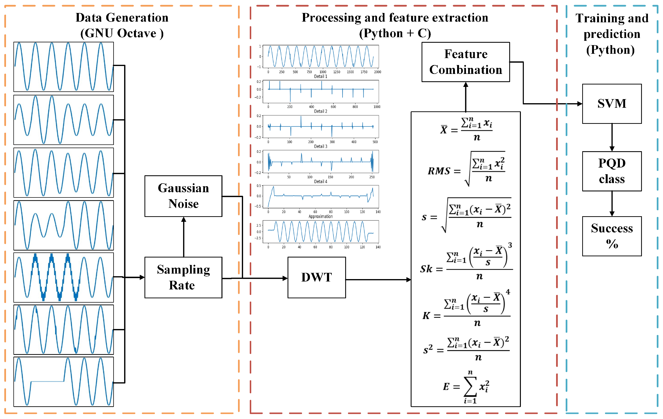
4. Materials and Methods

The proposed methodology can be seen in Figure 1, which consists of three parts; the first is the generation of signals in GNU Octave 9.3.0 using eight sampling frequencies and three levels of white Gaussian noise with SNR of 30, 40 and 50 dB; the second part is the processing and feature extraction using the mother wavelets dmey, bior1.1, db4, db28, and rbio3.1, applying between four and seven decomposition levels, from which different feature combinations will be extracted and used in the training and prediction stage using an SVM classifier.

4.1. Data Generation

Waveforms containing PQDs were created using mathematical models used in [7,26,29]. Between 1404 and 1521 signals were created for each of the seven PQ events, having noiseless and signals with SNR of 30, 40 and 50 dB of WGN, which are some of the SNR values used in [6,11,12,13,14], to which the following classes were assigned, Sine (C1), Sag (C2), Transient Oscillation (C3), Swell (C4), Flicker (C5), Interruption (C6) and Notch (C7), being a total of 9558 signals for each noise level. The sampling rates ($f_s$) used were 3.2, 5, 6.4, 8, 9.6, 15, 20 and 30 kHz, as suggested in [6,7,16,17,18,19], the frequency of the sinusoidal signal (w) was 60 Hz, which is the one used in Mexico, and the time window used was 12 cycles or 200 ms, which is the most used according to the IEEE 1159-2009 standard [30].

Table 1. Mathematical models.

Name	Class	Mathematical Model	Parameters
Normal	C1	$x(t)=Asin(\omega t)[1-\alpha (u(t-t_1)-u(t-t_2))]$	$-0.08\le \alpha \le 0.08$
			$0.5T\le t_2-t_1\le 12T$
Sag	C2	$x(t)=Asin(\omega t)[1-\alpha (u(t-t_1)-u(t-t_2))]$	$0.1\le \alpha \le 0.9$
			$0.5T\le t_2-t_1\le 12T$
Transient Oscillation	C3	$x(t)=Asin(\omega t)+[\alpha sin(w_{o}t)(exp(-0.001({\displaystyle \frac{t-t_1}{\tau }})))(u(t-t_1)-u(t-t_2))]$	$0.1\le \alpha \le 0.8$
			$0.5T\le t_2-t_1\le 3T$
			$8\mathrm{ms}\le \tau \le 40\mathrm{ms}$
		$w_o=2\pi f_n$	$300\mathrm{Hz}\le f_n\le 900\mathrm{Hz}$
Swell	C4	$x(t)=Asin(\omega t)[1+\alpha (u(t-t_1)-u(t-t_2))]$	$0.1\le \alpha \le 0.8$
			$0.5T\le t_2-t_1\le 12T$
Flicker	C5	$x(t)=Asin(\omega t)[1+\alpha sin(w_{o}t)]$	$0.1<\alpha \le 0.2$
		$w_o=2\pi \beta$	$6\mathrm{Hz}\le \beta \le 25\mathrm{Hz}$
Interruption	C6	$x(t)=Asin(\omega t)[1-\alpha (u(t-t_1)-u(t-t_2))]$	$0.9<\alpha \le 1$
			$0.5T\le t_2-t_1\le 12T$
Notch	C7	${\displaystyle x(t)=Asin(\omega t)-sign[\alpha sin(\omega t)\ast \sum _{n=0}^{9}u(t-(t_1+0.02n))-u(t-(t_2+0.02n))]}$	$0.1\le \alpha \le 0.4$
			$0.01T\le t_2-t_1\le 0.05T$

shows the mathematical models and the ranges of values used, where an amplitude (A) equal to one is used, the duration of the disturbances is controlled by a pair of step functions ($u\left(t\right)$) with shifts, $\alpha$ performs the changes in magnitude, and $f_n$ and $\beta$, are frequency values.

4.2. Processing and Feature Extraction

The second part of the methodology consists of processing and feature extraction, a very important part as it prepares the data for training. At the processing stage, decomposition levels four to seven were tested using the $PyWavelets$ library [31], as it offers a wide variety of different wavelets and good performance. As suggested in [32], the $dmey$ mother wavelet was used to perform tests for the feature selection.

In feature extraction, the relevant information of the signal is obtained to reduce the input vector that will be used in the training of the classifier. In this work, seven statistical properties were selected to be calculated at each of the decomposition levels obtained by applying DWT, which were mean ($\overline{X}$), Root Mean Square ($RMS$), standard deviation (s), kurtosis (K), skewness ($Sk$), variance ($s^2$) and energy (E). For each decomposition level, sampling rate and noise, all combinations were tested using between three and seven of the features shown in

Table 2. Equations of selected features.

Feature	Equation	Feature	Equation
Mean (1)	$\overline{X}={\displaystyle \frac{{\displaystyle \sum _{i=1}^n{x}_i}}{n}}$	Root Mean Square (2)	$RMS=\sqrt{{\displaystyle \frac{{\displaystyle \sum _{i=1}^n{x}_i^2}}{n}}}$
Standard Deviation (3)	$s=\sqrt{{\displaystyle \frac{{\displaystyle \sum _{i=1}^n{\left(x_i-\overline{X}\right)}^2}}{n}}}$	Symmetry (4)	$Sk={\displaystyle \frac{{\displaystyle \sum _{i=1}^n{\left(\frac{x_i-\overline{X}}{s}\right)}^3}}{n}}$
Kurtosis (5)	$K={\displaystyle \frac{{\displaystyle \sum _{i=1}^n{\left(\frac{x_i-\overline{X}}{s}\right)}^4}}{n}}$	Variance (6)	$s^2={\displaystyle \frac{{\displaystyle \sum _{i=1}^n{\left(x_i-\overline{X}\right)}^2}}{n}}$
Energy (7)	${\displaystyle E=\sum _{i=1}^n{x}_i^2}$

in order to obtain the configurations that obtained the best performance. For noisy signals, tests were also performed by eliminating between one and four of the decomposition levels that contained the highest frequencies to minimize the noise in the waveform. This removal of the highest frequencies improves the quality of the information extracted with the features by removing the randomness of the noise and trying to reduce the amount of data that must be processed when using high sampling rates.

4.3. Training and Prediction

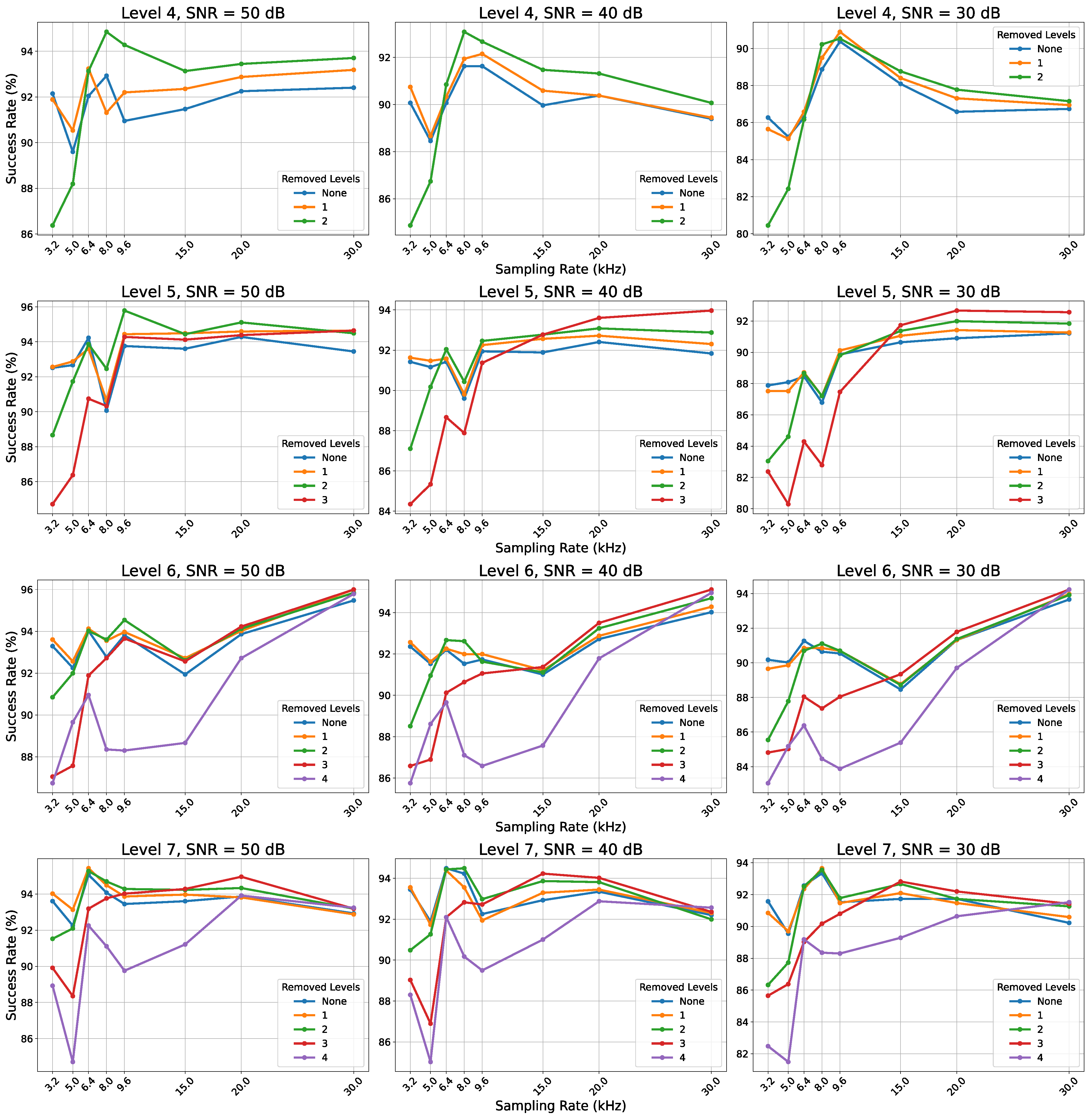
The SVM OAA classifier with polynomial kernel was chosen, which allows the modification of three important parameters: regularization coefficient (C), kernel coefficient ($\gamma$), bias (b) and polynomial degree [33]. The coefficient C controls the size of the margin, a large value of this parameter causes the margin to be smaller, and, consequently, a smaller number of errors are allowed. The $\gamma$ value determines the influence on the final decision of each of the inputs during training. In this work, a value of $\gamma$ equal to 0.04 was used, calculated according to the size of the input vectors; a value of b equal to zero; a degree three for the polynomial kernel, since tests using higher degrees did not present an improvement and increased the training time greatly; and a coefficient C equal to two, since tests using higher values did not improve performance and placing high values can cause the margin to be too small and overfit the data. The total data were divided into 80% for training and 20% for validation. For the implementation of the classifier, the $Scikit-Learn$ library was used since it is based on $LIBSVM$ [34], which is the preferred option in several programming languages.

5. Results

The results shown in Figure 2 were obtained from tests carried out with all feature combinations and decomposition levels for noiseless signals, where an irregular behavior is observed at the lowest sampling rates; then, the $f_s$ of 9.6 kHz is observed to obtain the best results for any level of decomposition. After that, the increase in the sampling frequency decreases the performance of the classifiers, so the increase in the decomposition levels does not greatly improve the highest success rate obtained in noiseless conditions. Using six and seven levels of decomposition gives the best results at almost all frequencies other than 9.6 kHz, while using four and five levels of decomposition gives the worst results for sampling frequencies other than 9.6 kHz.

The best performances for each sampling frequency, noise level, and decomposition level are shown in Figure 3; the effect of eliminating the highest frequencies is also shown, which follow the next order from highest to lowest frequency: d1, d2, d3 and d4. Using four levels of decomposition, removing the higher frequencies provides an improvement in performance for frequencies greater than 6.4 kHz. For the three noise levels, the best results are obtained between 8 and 9.6 kHz; for signals with SNR of 50 and 40 dB, the best configuration results from removing d1 and d2, while for 30 dB, the best result is obtained by removing d1. Using five levels of decomposition, the best performance on signals with an SNR of 50 dB is obtained at an $f_s$ of 9.6 kHz, and the use of higher frequencies worsens the success; for 40 and 30 dB, the best successes are obtained at the highest sampling rate by eliminating d1, d2, and d3. For five, six and seven levels of decomposition, it is observed that removal beyond d2 requires a higher sampling rate to obtain good results. With six levels of decomposition, an upward trend is observed from an $f_s$ of 15 kHz, obtaining the best results at 30 kHz, eliminating up to d3 and d4. Finally, with seven levels of decomposition, it is observed that for the three noise levels, there is an increase in performance at an $f_s$ between 6.4 and 8 kHz; subsequently, a small decrease in accuracy is observed as the sampling rate increases.

Based on the results shown in Figure 3, the configurations that obtained the best percentage of success for each noise level and sampling rate were chosen.

Table 3. Best algorithm settings for each noise level and sampling rate.

${\mathbf{f}}_{\mathbf{s}}$ (kHz)	DWT Level	Levels Removed	Noise Level (SNR)	Comb.	Success %	DWT Level	Levels Removed	Noise Level (SNR)	Comb.	Success %
3.2	5	-	-	1, 3, 4, 5, 6	97.44	7	1	50	2, 4, 5, 6	94.02
5	6	-	-	1, 2, 3, 4, 5, 6	96.18	7	1	50	1, 3, 5, 6	93.14
6.4	6	-	-	3, 4, 5, 6	98.95	7	1	50	1, 2, 3, 4, 5, 6	95.42
8	7	-	-	1, 2, 3, 4, 5, 6	97.49	4	2	50	3, 5, 6	94.85
9.6	5	-	-	1, 5, 6	99.90	5	2	50	3, 5, 6	95.79
15	7	-	-	1, 3, 4, 5, 6	97.39	5	1	50	1, 3, 4, 5, 6	94.49
20	7	-	-	1, 2, 3, 5, 6	97.04	5	2	50	3, 4, 5, 6	95.11
30	7	-	-	4, 5, 6	97.54	6	1	50	3, 5, 6	96.00
3.2	7	-	30	3, 4, 5, 6	91.58	7	1	40	1, 2, 4, 5, 6	93.55
5	6	-	30	2, 4, 5, 6	90.02	7	-	40	2, 3, 4, 5, 6	91.89
6.4	7	-	30	1, 2, 3, 5, 6	92.56	7	-	40	1, 2, 3, 4, 5, 6	94.49
8	7	1	30	1, 2, 3, 5, 6	93.66	7	2	40	1, 3, 5, 6	94.49
9.6	7	2	30	1, 2, 4, 5, 6	91.78	7	2	40	3, 4, 5, 6	92.98
15	7	3	30	1, 4, 5, 6	92.82	7	3	40	1, 2, 4, 5, 6	94.23
20	5	3	30	1, 3, 5, 6	92.67	7	3	40	1, 3, 5, 6	94.02
30	6	3	30	1, 2, 3, 4, 5, 6	94.23	6	3	40	3, 4, 5, 6	95.11

shows the information on the level of decomposition that must be performed with the DWT, the combination of features, and up to what level of decomposition they must be eliminated to obtain the best results with the proposed algorithm.

From the configurations shown in Table 3, tests were performed by changing the mother wavelet dmey to bior4.4, rbio3.1, db4, and db28, in order to analyze whether this change in the processing stage affected the performance of the algorithm. Figure 4 shows the comparison of the success percentages for the different noise levels and sampling rates obtained using the five mother wavelets.

After performing the tests with the mother wavelets, the results shown in

Table 4. Best algorithm settings and runtimes for each noise level.

${\mathbf{f}}_{\mathbf{s}}$ (kHz)	SNR	Mother Wavelet	DWT Level	Levels Removed	Comb.	Success Rate								Run-Time ($\mathsf{\mu }$s)
						AVG	C1	C2	C3	C4	C5	C6	C7
3.2	-	dmey	5	-	1, 3, 4, 5, 6	97.4	94.7	96.7	99.7	98.6	100	91.8	100	239
5	-	db28	6	-	1, 2, 3, 4, 5, 6	96.2	93.1	93.9	100	97.6	100	88.4	99.7	277
6.4	-	dmey	6	-	3, 4, 5, 6	98.9	100	97.5	100	100	100	95	99.7	294
8	-	bior4.4	7	-	1, 2, 3, 4, 5, 6	98.3	95.1	96.5	99.7	100	100	96.8	100	212
9.6	-	dmey	5	-	1, 5, 6	99.9	100	100	100	100	100	99.6	99.7	323
15	-	dmey	7	-	1, 3, 4, 5, 6	97.4	93.7	96.2	99.7	100	100	91.5	100	445
20	-	dmey	7	-	1, 2, 3, 5, 6	97	91.6	97.3	100	100	99.3	90.8	100	527
30	-	db28	7	-	4, 5, 6	99.6	98.6	100	100	100	100	98.8	99.7	661
3.2	50	bior4.4	7	1	2, 4, 5, 6	94.3	80.6	94.7	100	97.9	100	90.3	100	314
5		rbio3.1	7	1	1, 3, 5, 6	93.9	82.3	97.3	100	99.3	97.7	85.7	99.3	306
6.4		dmey	7	1	1, 2, 3, 4, 5, 6	95.4	84.8	96.7	100	97.9	100	90.6	100	544
8		dmey	4	2	3, 5, 6	94.9	86.9	97	100	97.2	96.9	88.3	100	387
9.6		dmey	5	2	3, 5, 6	95.8	86.7	97.5	100	99.3	99.2	89.9	100	401
15		dmey	5	1	1, 3, 4, 5, 6	94.5	83.7	95.4	100	97.5	98.8	88.8	100	477
20		dmey	5	2	3, 4, 5, 6	95.1	86.8	98.3	100	97.9	96.2	89.1	100	399
30		dmey	6	1	3, 5, 6	96	88.4	97.2	100	98	98.5	91.4	100	482
3.2	40	dmey	7	1	1, 2, 4, 5, 6	93.6	76.6	95.4	100	99.6	98.5	90.7	100	566
5		rbio3.1	7	-	2, 3, 4, 5, 6	93.2	80.1	97.2	100	99.3	96.3	85.7	99.3	435
6.4		db28	7	-	1, 2, 3, 4, 5, 6	94.7	83.4	95	100	98.6	100	88.6	100	698
8		rbio3.1	7	2	1, 3, 5, 6	95.4	86.8	96.6	100	97.4	99.6	89.5	99.6	233
9.6		dmey	7	2	3, 4, 5, 6	93	85	92.2	100	91.8	97	86.8	99.6	477
15		dmey	7	3	1, 2, 4, 5, 6	94.2	81.2	96	100	98.9	100	87.6	100	448
20		dmey	7	3	1, 3, 5, 6	94	82.6	96.4	100	98.2	98.5	86.3	100	449
30		dmey	6	3	3, 4, 5, 6	95.1	84	98.7	100	98.2	99.2	88.9	100	384
3.2	30	db4	7	-	3, 4, 5, 6	91.9	76.4	91.2	100	97.8	97	86.1	100	443
5		rbio3.1	6	-	2, 4, 5, 6	93	79.8	96.4	100	97.9	98.1	86.4	97.4	429
6.4		rbio3.1	7	-	1, 2, 3, 5, 6	93.7	79.9	99.5	100	97.9	99.2	86.4	98.5	434
8		rbio3.1	7	1	1, 2, 3, 5, 6	94.6	84.4	95	100	97.6	99.2	88.5	99.6	300
9.6		bior4.4	7	2	1, 2, 4, 5, 6	93.2	79.8	91.2	99.6	97.1	99.2	89.6	99.3	256
15		dmey	7	3	1, 4, 5, 6	92.8	78.3	92.1	100	98.6	98.9	86.5	99.6	439
20		db4	5	3	1, 3, 5, 6	93.9	86.8	94.1	100	95.3	96.6	86.7	100	146
30		bior4.4	6	3	1, 2, 3, 4, 5, 6	95.2	86.4	97.9	100	99.3	97.7	88.2	99.6	208

were obtained, where the best configurations of sampling frequency, mother wavelet, decomposition level, and filtering are shown, obtaining success percentages between 91.9 and 99.9, taking into account all sampling frequencies and noise levels. Although the optimizations were performed using the mother wavelet $dmey$, there are cases in which better results were obtained using another wavelet. The worst classified classes were C1 and C6 for all cases, while the best classified were C3 and C7. Tests were performed on a laptop with an i7-12650H processor with 16 GB of RAM to obtain execution times, where times less than 700 $\mathsf{\mu }$s were obtained for processing and classification. The processing phase achieved times between 53 and 583 $\mathsf{\mu }$s depending on the number of features, the mother wavelet, and the decomposition levels; the classification phase achieved times between 78 and 115 $\mathsf{\mu }$s; and the training time was between 0.34 and 8.08 s for a total of 7671 waveforms. Table 4 shows the configurations that obtained the best success for each noise level and its runtime.

6. Discussion

The success rates obtained show that the proposed algorithm is capable of classifying waveforms containing PQDs and white Gaussian noise. Removing higher frequencies after applying DWT was shown to improve the algorithm’s performance for all three noise levels; however, it requires a higher sampling rate to deliver good results.

The results shown in Figure 2 and Figure 3 demonstrate that the sampling frequency can affect the performance of algorithms for PQD classification. Unlike the results obtained in [16], the proposed algorithm does not present a tendency for a large increase at first and then maintaining a success rate without major changes as the sampling rate increases in noiseless scenarios. However, this behavior does occur when applying six levels of decomposition to noisy signals.

From the results shown in Table 4, it is obtained that the best configuration for noiseless signals is an $f_s$ of 9.6 kHz, five levels of decomposition without eliminating any, a $dmey$ mother wavelet, and using mean, kurtosis, and variance as features. For signals with an SNR of 50 dB, the best setting is an $f_s$ equal to 30 kHz, a $dmey$ mother wavelet, six levels of decomposition removing d1, and using standard deviation, kurtosis, and variance as features. For signals with SNR of 40 dB, the best configuration is an 8 kHz of sampling rate, a rbio3.1 mother wavelet, seven levels of decomposition removing d1 and d2, and using mean, standard deviation, kurtosis, and variance as features. Finally, for signals with an SNR of 30 dB; the best configuration is a sampling rate of 30 kHz; a bior4.4 mother wavelet, six levels of decomposition removing d1, d2 and d3; and using mean, RMS, standard deviation, kurtosis, symmetry, and variance as features. The execution time of less than 700 $\mathsf{\mu }$s achieved with the algorithm makes it a good option for implementation on single-board computers for real-time classification. Furthermore, since it is made from $Python$ and C, it can be easily migrated between different devices.

The appearance of mother wavelets, different from $dmey$ in Table 3, shows that it can affect the success of the algorithm since the shape of a particular wavelet could better adapt to the analyzed data. It could extract more relevant information from the waveforms and perform better noise filtering.

The algorithm demonstrated good performance in classifying disturbances involving frequency in noisy environments. The decrease in the accuracy of events involving a change in amplitude in these environments may be because noise is not eliminated at all levels of decomposition by the processing performed. Because the difference in amplitudes between classes is minimal, different characteristics could be used. An adjustment could be made in the size of the margin to reduce errors in the decision limits, or a classification could be made based on the maximum and minimum values.

Although there are works such as Refs. [2,6] in which a better percentage of success is obtained in the classification of noisy signals, these require more complex processing and greater computational resources. So the execution times in the real-time classification of PQDs could be affected. On the other hand, the proposed algorithm obtained better performance in the classification of noiseless signals.

The proposed algorithm could be a suitable option for classifying real signals, although the tests were carried out with waveforms generated from mathematical models. This capacity to classify actual signals is because removing the highest frequencies of the signal would help eliminate most of the noise coming from the measuring devices and the electrical network. It has also shown good performance in noisy environments. However, in reality, combinations of disturbances occur, so this type of event would have to be added. Therefore, the classifier would have to be adjusted based on real signals to evaluate whether the algorithm could deliver good performance under these conditions.

In future work, a search for new sampling rates that help improve the performance of the algorithm can be carried out. The addition of more types of PQDs, tests with different mother wavelets, and the implementation of the algorithm in single-board computers for real-time classification can also be performed.

References

1. Thiyagarajan, V.; Subramaniam, N.P. Wavelet approach and support vector networks based power quality events recognition and categorisation. In Proceedings of the 2016 International Conference on Signal Processing, Communication, Power and Embedded System (SCOPES), Paralakhemundi, India, 3–5 October 2016; pp. 1667–1671. [Google Scholar] [CrossRef]
2. Mishra, S.; Mallick, R.; Gadanayak, D.A.; Nayak, P.; Sharma, R.; Panda, G.; Al-Numay, M.; Siano, P. Real Time Intelligent Detection of PQ Disturbances With Variational Mode Energy Features and Hybrid Optimized Light GBM Classifier. IEEE Access 2024, 12, 47155–47172. [Google Scholar] [CrossRef]
3. Suganthi, S.T.; Vinayagam, A.; Veerasamy, V.; Deepa, A.; Abouhawwash, M.; Thirumeni, M. Detection and classification of multiple power quality disturbances in Microgrid network using probabilistic based intelligent classifier. Sustain. Energy Technol. Assess. 2021, 47, 101470. [Google Scholar] [CrossRef]
4. Mahela, O.P.; Shaik, A.G.; Khan, B.; Mahla, R.; Alhelou, H.H. Recognition of Complex Power Quality Disturbances Using S-Transform Based Ruled Decision Tree. IEEE Access 2020, 8, 173530–173547. [Google Scholar] [CrossRef]
5. Markovska, M.; Taskovski, D.; Kokolanski, Z.; Dimchev, V.; Velkovski, B. Real-Time Implementation of Optimized Power Quality Events Classifier. IEEE Trans. Ind. Appl. 2020, 56, 3431–3442. [Google Scholar] [CrossRef]
6. Enshaee, A.; Enshaee, P. A New S-Transform-Based Method for Identification of Power Quality Disturbances. Arab. J. Sci. Eng. 2018, 43, 2817–2832. [Google Scholar] [CrossRef]
7. Samanta, I.S.; Rout, P.K.; Mishra, S. An optimal extreme learning-based classification method for power quality events using fractional Fourier transform. Neural Comput. Appl. 2021, 33, 4979–4995. [Google Scholar] [CrossRef]
8. Rahul. Multiple power quality events recognition and classification based on adaptive Eigen-based type-2 fuzzy logic algorithm. Iran J. Comput. Sci. 2022, 5, 55–68. [Google Scholar] [CrossRef]
9. Samanta, I.S.; Rout, P.K.; Mishra, S. Power Quality Events Recognition Using S-Transform and Wild Goat Optimization-Based Extreme Learning Machine. Arab. J. Sci. Eng. 2020, 45, 1855–1870. [Google Scholar] [CrossRef]
10. Motlagh, S.; Akbari Foroud, A. Power quality disturbances recognition using adaptive chirp mode pursuit and grasshopper optimized Support Vector Machines. Measurement 2021, 168, 108461. [Google Scholar] [CrossRef]
11. Khokhar, S.; Zin, A.M.; Mokhtar, A.; Bhayo, M.; Naderipour, A. Automatic classification of single and hybrid power quality disturbances using Wavelet Transform and Modular Probabilistic Neural Network. In Proceedings of the 2015 IEEE Conference on Energy Conversion (CENCON), Johor Bahru, Malaysia, 19–20 October 2015; pp. 457–462. [Google Scholar] [CrossRef]
12. Jian, X.; Wang, X. A novel semi-supervised method for classification of power quality disturbance using generative adversarial network. J. Intell. Fuzzy Syst. 2021, 40, 3875–3885. [Google Scholar] [CrossRef]
13. Chiam, D.H.; Lim, K.H.; Law, K.H. LSTM power quality disturbance classification with wavelets and attention mechanism. Electr. Eng. 2023, 105, 259–266. [Google Scholar] [CrossRef]
14. Wang, J.; Zhang, D.; Zhou, Y. Ensemble deep learning for automated classification of power quality disturbances signals. Electr. Power Syst. Res. 2022, 213, 108695. [Google Scholar] [CrossRef]
15. Khetarpal, P.; Nagpal, N.; Siano, P.; Al-Numay, M. Power quality disturbance signal segmentation and classification based on modified BI-LSTM with double attention mechanism. IET Gener. Transm. Distrib. 2024, 18, 50–62. [Google Scholar] [CrossRef]
16. Eisenmann, A.; Streubel, T.; Rudion, K. PQ classification by way of parallel computing—A sensitivity analysis for a real-time LSTM approach using waveform and RMS data. In Proceedings of the 2019 IEEE Milan PowerTech, Milan, Italy, 23–27 June 2019; pp. 1–6. [Google Scholar] [CrossRef]
17. Liu, J.; Tang, Q.; Ma, J.; Qiu, W. FFNet: An automated identification framework for complex power quality disturbances. Electr. Power Syst. Res. 2022, 208, 107866. [Google Scholar] [CrossRef]
18. Achlerkar, P.D.; Samantaray, S.R.; Sabarimalai Manikandan, M. Variational Mode Decomposition and Decision Tree Based Detection and Classification of Power Quality Disturbances in Grid-Connected Distributed Generation System. IEEE Trans. Smart Grid 2018, 9, 3122–3132. [Google Scholar] [CrossRef]
19. Karasu, S.; Saraç, Z. Investigation of power quality disturbances by using 2D discrete orthonormal S-transform, machine learning and multi-objective evolutionary algorithms. Swarm Evol. Comput. 2019, 44, 1060–1072. [Google Scholar] [CrossRef]
20. Grossmann, A.; Morlet, J. Decomposition of Hardy Functions into Square Integrable Wavelets of Constant Shape. SIAM J. Math. Anal. 1984, 15, 723–736. [Google Scholar] [CrossRef]
21. Erişti, H.; Demir, Y. Automatic classification of power quality events and disturbances using wavelet transform and Support Vector Machines. IET Gener. Transm. Distrib. 2012, 6, 968–976. [Google Scholar] [CrossRef]
22. Nieto, N.; Orozco, D.M. El uso de la transformada Wavelet discreta en la reconstrucción de señales senosoidales. Sci. Tech. 2008, 1, 381–386. [Google Scholar]
23. Mallat, S. A theory for multiresolution signal decomposition: The wavelet representation. IEEE Trans. Pattern Anal. Mach. Intell. 1989, 11, 674–693. [Google Scholar] [CrossRef]
24. Lester, M. Introducción a Wavelets, Buenos Aires, Argentina, 2006. 20 February. Available online: https://users.exa.unicen.edu.ar/catedras/escuelapav/cursos/wavelets.htm (accessed on 1 February 2025).
25. Cortes, C.; Vapnik, V. Support-vector networks. Mach. Learn. 1995, 20, 273–297. [Google Scholar] [CrossRef]
26. Thirumala, K.; Pal, S.; Jain, T.; Umarikar, A.C. A classification method for multiple power quality disturbances using EWT based adaptive filtering and multiclass SVM. Neurocomputing 2019, 334, 265–274. [Google Scholar] [CrossRef]
27. Rodrigues Junior, W.L.; Borges, F.A.S.; Veloso, A.F.d.S.; Rabêlo, R.d.A.L.; Rodrigues, J.J.P.C. Low voltage smart meter for monitoring of power quality disturbances applied in Smart Grid. Measurement 2019, 147, 106890. [Google Scholar] [CrossRef]
28. Bishop, C.M. Pattern Recognition and Machine Learning (Information Science and Statistics), 1st ed.; Springer: Berlin/Heidelberg, Germany, 2007. [Google Scholar]
29. Panigrahi, R.R.; Mishra, M.; Nayak, J.; Shanmuganathan, V.; Naik, B.; Jung, Y.A. A power quality detection and classification algorithm based on FDST and hyper-parameter tuned light-GBM using memetic firefly algorithm. Measurement 2022, 187, 110260. [Google Scholar] [CrossRef]
30. IEEE Std 1159-2009; IEEE Recommended Practice for Monitoring Electric Power Quality, (Revision of IEEE Std 1159-1995). Institute of Electrical and Electronics Engineers: New York, NY, USA, 2009; pp. 1–94. [CrossRef]
31. Lee, G.R.; Gommers, R.; Waselewski, F.; Wohlfahrt, K.; Leary, A. PyWavelets: A Python package for wavelet analysis. J. Open Source Softw. 2019, 4, 1237. [Google Scholar] [CrossRef]
32. Medina-Molina, J.A.; Arzate-Rueda, B.; Reyes-Archundia, E.; Gutiérrez-Gnecchi, J.A.; Olivares-Rojas, J.C.; Rodríguez-Herrejón, J.A.; Guerrero-Rodríguez, N.F. Execution time comparison of algorithms to classify power quality disturbances in single board computers. In Proceedings of the 2024 IEEE International Autumn Meeting on Power, Electronics and Computing (ROPEC), Ixtapa, Mexico, 1–2 November 2024; Volume 8, pp. 1–6. [Google Scholar] [CrossRef]
33. Pedregosa, F.; Varoquaux, G.; Gramfort, A.; Michel, V.; Thirion, B.; Grisel, O.; Blondel, M.; Prettenhofer, P.; Weiss, R.; Dubourg, V.; et al. Scikit-learn: Machine Learning in Python. J. Mach. Learn. Res. 2011, 12, 2825–2830. [Google Scholar]
34. Chang, C.C.; Lin, C.J. LIBSVM: A library for Support Vector Machines. ACM Trans. Intell. Syst. Technol. 2011, 2, 1–27. [Google Scholar] [CrossRef]
Figure 1. Proposed methodology for PQD classification.
Computers 14 00138 g001
Figure 2. Comparison of success rates obtained in noiseless signals applying DWT with different decomposition levels.
Computers 14 00138 g002
Figure 3. Comparison of the performance of SVM classifiers when eliminating the highest frequencies by applying DWT with different levels of decomposition to noisy signals.
Computers 14 00138 g003
Figure 4. Comparison of the success rates obtained using different mother wavelets.
Computers 14 00138 g004