A Secure Cooperative Adaptive Cruise Control Design with Unknown Leader Dynamics Under False Data Injection Attacks

Abstract

The combination of connectivity and automation allows connected and autonomous vehicles (CAVs) to operate autonomously using advanced on-board sensors while communicating with each other via vehicle-to-vehicle (V2V) technology to enhance safety, efficiency, and mobility. One of the most promising features of CAVs is cooperative adaptive cruise control (CACC). This system extends the capabilities of conventional adaptive cruise control (ACC) by facilitating the exchange of critical parameters among vehicles to enhance safety, traffic flow, and efficiency. However, increased connectivity introduces new vulnerabilities, making CACC susceptible to cyber-attacks, including false data injection (FDI) attacks, which can compromise vehicle safety. To address this challenge, we propose a secure observer-based control design leveraging Lyapunov stability analysis, which is capable of mitigating the adverse impact of FDI attacks and ensuring system safety. This approach uniquely addresses system security without relying on a known lead vehicle model. The developed approach is validated through simulation results, demonstrating its effectiveness.

1. Introduction

The continuous growth of the automobile industry, coupled with rapid urbanization, has resulted in a substantial increase in the number of vehicles. Consequently, modern transportation systems are facing different challenges, including a rise in traffic accidents, severe traffic congestion, increased energy consumption, and heightened levels of pollution [1]. Early applications developed to address these challenges relied on local sensors, such as radar and cameras, to enable vehicle autonomy. While these technologies allowed vehicles to detect and respond to their immediate environment and support real-time decision-making, they offer only a limited level of safety because of the constrained sensing ranges and the complexities of data processing [2,3].

To overcome these limitations, additional sources of data were essential to expand surrounding perception across a wider area. Vehicle-to-vehicle (V2V) communication has been introduced as a solution to address these limitations. By enabling vehicles to share critical information on acceleration, speed, position, and trajectory, V2V communication offers a more comprehensive understanding of the surrounding environment [4]. Therefore, the integration of automated vehicles (AVs) and connected vehicles (CVs) as connected and autonomous vehicles (CAVs) has the potential to address all above-mentioned challenges, resulting in improvements in safety and efficiency and reducing traffic congestion [5,6,7].

Cooperative adaptive cruise control (CACC) as a key feature of CAVs, has enhanced the capabilities of adaptive cruise control (ACC) to improve safety, traffic flow, and energy efficiency through cooperative maneuvers [8,9]. In CACC systems, vehicles exchange information with one another within the network via V2V communications, which results in several key benefits including improved reaction times in vehicles, enhanced safety, increased traffic flow efficiency, fuel efficiency and reduced emissions, and string stability in vehicles’ platoons [9,10,11,12].

Although CAVs and CACC offer numerous benefits, their heavy reliance on V2V communications makes vehicles susceptible to cyber-attacks such as false data injection (FDI) attacks. These threats can compromise the reliability of observations used in decision-making process [13,14,15]. Therefore, it is necessary to develop a secure CACC algorithm to address and mitigate these attacks effectively.

The design of CACC has been widely studied in various studies; each of them has addressed different objectives and operated under different assumptions and conditions. In [16], the research utilized deep reinforcement learning (DRL) to improve the performance of CACC, comparing its effectiveness to traditional model-based approaches. The research aimed to minimize both distance error and energy consumption while ensuring safety. A model predictive control (MPC) approach for CACC was designed in [17]. In this study, by predicting traffic and integrating fuel-efficient control, the system minimized fuel usage and prevented collisions. In [18], a dynamic event-triggered communication mechanism (DECM) approach was introduced for CACC systems. This method was used to conserve constrained V2V communication resources. By implementing DECM, the frequency of measured velocity and acceleration data required for transmission to following vehicles is minimized. In [19], the researchers concentrated on a different aspect of CACC, specifically string stability. The main objective of this study was to tackle the challenge of maintaining string stability as inter-vehicle time gaps decrease. However, none of the mentioned studies addressed the impact of FDI attacks on the communication channel of the CACC system.

The development of CACC under FDI attacks has been considered in a limited number of studies. A recent study analyzed the effects of FDI attacks on CACC [20]. This research examined FDI attacks within the CACC communication channel, including ghost vehicle injections aimed at disrupting system performance. To detect and locate these attacks, the authors developed a partial differential equation (PDE)-based model as the dynamic model for vehicles and designed a PDE observer. By leveraging Lyapunov stability theory, they validated the observer’s convergence, ensuring robust detection of attacks even in the presence of noise. The effects of FDI attacks were also considered in [21]. This research employed a hybrid approach, combining both model-based and learning-based methods to estimate FDI attacks. Additionally, it introduced a Lyapunov-based controller designed to reduce the adverse effects of FDI attacks, measurement noise, and external disturbances in CACC, ensuring the maintenance of a safe distance between vehicles. Further research on CACC under FDI attacks was presented in [22]. This study addressed the effects of FDI attacks, input time-varying delays, external disturbances, and measurement noise by developing a nonlinear controller, observer, and NN-based attack estimators. However, all of the mentioned papers assumed that the dynamic model of the lead vehicle is known, while accessing the dynamic model of the lead vehicle presents a significant challenge, which is a key focus of this paper.

The contributions of our paper are as follows: (i) A novel observer-based control for CACC was developed that is resilient against injected FDI attacks into both transmitted velocity and control signals. (ii) The proposed approach operates effectively without relying on the dynamic model of the lead vehicle. (iii) The proposed nonlinear observer was designed to estimate FDI attacks in real time. (iv) Additionally, we provided a comprehensive Lyapunov stability analysis for both the proposed nonlinear controller and the observer. (v) Finally, we validated the developed method through simulations to demonstrate its effectiveness.

The structure of the paper is organized as follows: Section 2 presents a dynamic model of the lead and following vehicles. The problem statement is detailed in Section 3. Section 4 presents an overview of the proposed solution, including observer design, control design, and estimation of FDI attacks. The stability analysis of the proposed observer and controller is discussed in Section 5. Section 6 demonstrates the results, and the paper concludes with a summary in Section 7.

2. Models of Dynamics

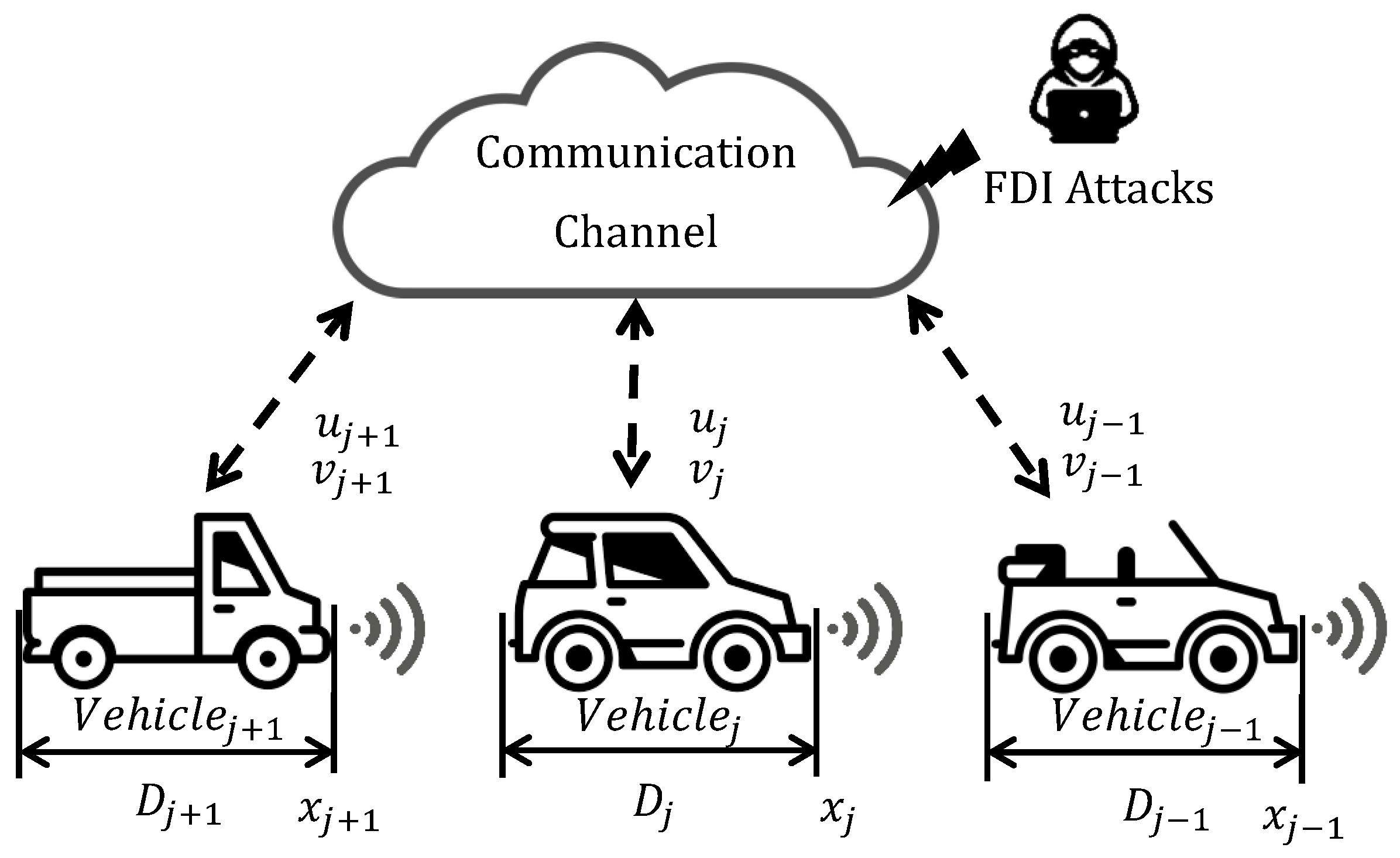
Figure 1 illustrates a string of vehicles, each equipped with the CACC feature. In this configuration, each vehicle follows its respective leader. Here, we assumed n vehicles in the platoon, where $j\in \{2,\cdots ,n\}$ denotes a following vehicle, while $j-1$ denotes its respective leader. Each follower vehicle j receives data from its leader $j-1$ including the leader’s control and velocity signals. However, during the transmission process via the wireless communication channel, an adversary may gain access and inject falsified data into the control and velocity signals. As a result, the following vehicle receives corrupted data. Additionally, each following vehicle uses a radar sensor to measure the position of its leader. The vehicles in this string are heterogeneous, meaning they are different models and not uniform in design. The dynamic model of followers is described as

$$\left\{\begin{array}{c}{\dot{x}}_j\left(t\right)=v_j\left(t\right),\hfill \\ {\dot{v}}_j\left(t\right)=-b_j{v}_j\left(t\right)+c_j{u}_j\left(t\right),\hfill \end{array}\right.$$

(1)

where the position, velocity, and control signals of the follower are indicated as $x_j\left(t\right)\in \mathbb{R}$, $v_j\left(t\right)\in \mathbb{R}$, and $u_j\left(t\right)\in \mathbb{R}$, respectively. In addition, $b_j$ and $c_j$ are known constants, representing dynamic models of the following vehicle, which are calculated using experimental analysis [21]. In this paper, we considered that the lead vehicle follows a second-order dynamic model such as

$$\left\{\begin{array}{c}{\dot{x}}_{j-1}\left(t\right)=v_{j-1}\left(t\right),\hfill \\ {\dot{v}}_{j-1}\left(t\right)=-b_{j-1}{v}_{j-1}\left(t\right)+c_{j-1}{u}_{j-1}\left(t\right),\hfill \end{array}\right.$$

(2)

where the position, velocity, and control signals of the leader are indicated as $x_{j-1}\in \mathbb{R}$, $v_{j-1}\in \mathbb{R}$, and $u_{j-1}\in \mathbb{R}$, respectively. The parameters $b_{j-1}$ and $c_{j-1}$ are unknown.

FDI Attacks in Communication Channel

Each vehicle receives the velocity and control signals of its leader through a wireless communication channel while the transmitted data are experiencing FDI attacks. To show the effect of FDI attacks on the control and velocity signals of the leader, we define the below signals:

$$\left\{\begin{array}{c}{\overline{u}}_{j-1}\left(t\right)\triangleq u_{j-1}\left(t\right)+f_{j-1}\left(t\right),\hfill \\ {\overline{v}}_{j-1}\left(t\right)\triangleq v_{j-1}\left(t\right)+f_{j-1}\left(t\right),\hfill \end{array}\right.$$

(3)

where ${\overline{u}}_{j-1}\left(t\right)\in \mathbb{R}$ and ${\overline{v}}_{j-1}\left(t\right)\in \mathbb{R}$ are altered control and velocity signals of the leader which are received by follower, and $f_{j-1}\left(t\right)\in \mathbb{R}$ is the unknown, bounded, time-varying, and continuous FDI attacks.

Assumption 1.

An FDI attack is assumed to be bounded and differentiable such that $∥f_{j-1}\left(t\right)∥\le {\overline{f}}_{j-1}$, where $t\ge t_0$ and ${\overline{f}}_{j-1}$ is a positive known constant [22].

Considering (3), the following vehicle receives altered signals. To estimate the control and velocity signals of the lead vehicle, we define the below signals:

$$\left\{\begin{array}{c}{\widehat{u}}_{j-1}\left(t\right)\triangleq {\overline{u}}_{j-1}\left(t\right)-{\widehat{f}}_{j-1}\left(t\right),\hfill \\ {\widehat{v}}_{j-1}\left(t\right)\triangleq {\overline{v}}_{j-1}\left(t\right)-{\widehat{f}}_{j-1}\left(t\right),\hfill \end{array}\right.$$

(4)

where ${\widehat{u}}_{j-1}\left(t\right)\in \mathbb{R}$, ${\widehat{v}}_{j-1}\left(t\right)\in \mathbb{R}$, and ${\widehat{f}}_{j-1}\left(t\right)\in \mathbb{R}$ are an estimation of the leader’s control signal, an the estimation of leader’s velocity signal, and an estimation of the FDI attacks, respectively.

3. Problem Statement and Error Signals

The primary focus of this work is to develop a secure controller for CACC to mitigate the effects of FDI attacks, therefore ensuring a safe inter-vehicle distance. The CACC algorithm relies on real-time control and velocity signals from the lead vehicle. However, adversarial manipulations pose a significant challenge to this process, potentially leading to collisions. In addition, the lead vehicle’s model is unknown, which introduces further complexity in secure controller design. Therefore, a secondary purpose of this study is to develop an observer capable of estimating FDI attacks and the unknown parameters of the lead vehicle in real time. To quantify these objectives, we defined error signals as distance error, velocity error, and acceleration error.

The distance error signal $e_j\in \mathbb{R}$ is defined as

$$e_{x_j}\left(t\right)\stackrel{\Delta }{=}{x}_j\left(t\right)-x_{j-1}\left(t\right)+D_{j-1}+x_{d_j}\left(t\right),$$

(5)

where $D_{j-1}\in \mathbb{R}$ is the length of lead vehicle which is constant, and $x_{d_j}\in \mathbb{R}$ is the desired inter-vehicle distance.

Assumption 2.

The desired distance, as well as its first and second derivatives, is assumed to remain within the limits of predefined positive constants, $x_{d_j},{\dot{x}}_{d_j},{\ddot{x}}_{d_j}\in {\mathcal{L}}_{\infty }$ [23].

The velocity error signal $e_{v_j}\in \mathbb{R}$ is introduced as

$$\left\{\begin{array}{c}{e}_{v_j}\left(t\right)={\dot{e}}_{x_j}\left(t\right),\hfill \\ e_{v_j}\left(t\right)={\dot{x}}_j\left(t\right)-{\dot{x}}_{j-1}\left(t\right)+{\dot{x}}_{d_j}\left(t\right),\hfill \end{array}\right.$$

(6)

using (1) and (2), (6) changes to

$$e_{v_j}\left(t\right)=v_j\left(t\right)-v_{j-1}\left(t\right)+{\dot{x}}_{d_j}\left(t\right).$$

(7)

In addition, the acceleration error signal $e_{a_j}\in \mathbb{R}$ is introduced as

$$\left\{\begin{array}{c}{e}_{a_j}\left(t\right)={\dot{e}}_{v_j}\left(t\right),\hfill \\ e_{a_j}\left(t\right)={\dot{v}}_j\left(t\right)-{\dot{v}}_{j-1}\left(t\right)+{\ddot{x}}_{d_j}\left(t\right),\hfill \end{array}\right.$$

(8)

using (1) and (2), (8) changes to

$$\begin{array}{cc}\hfill e_{a_j}\left(t\right)=& -b_j{v}_j\left(t\right)+c_j{u}_j\left(t\right)+b_{j-1}{v}_{j-1}\left(t\right)\hfill \\ & -c_{j-1}{u}_{j-1}\left(t\right)+{\ddot{x}}_{d_j}\left(t\right),\hfill \end{array}$$

(9)

we can write (9) as

$$e_{a_j}\left(t\right)=-b_j{v}_j\left(t\right)+c_j{u}_j\left(t\right)+{\theta }_{j-1}\left(t\right)+{\ddot{x}}_{d_j}\left(t\right),$$

(10)

where ${\theta }_{j-1}\left(t\right)\in \mathbb{R}$ is the combination of all unknown terms in (9) and is defined as

$${\theta }_{j-1}\left(t\right)\stackrel{\Delta }{=}{b}_{j-1}{v}_{j-1}\left(t\right)-c_{j-1}{u}_{j-1}\left(t\right),$$

(11)

where the control and velocity signals of leader are unknown under FDI attacks. In addition, since the dynamic model of the lead vehicle is unknown, $b_{j-1}$ and $c_{j-1}$ are unknown.

To streamline the design process and stability analysis of the second-order system, an auxiliary error equation is introduced to derive the control signal as

$$r_j\left(t\right)\stackrel{\Delta }{=}{\widehat{e}}_{v_j}\left(t\right)+{\alpha }_j{\widehat{e}}_{x_j}\left(t\right),$$

(12)

where ${\alpha }_j\in {\mathbb{R}}_{>0}$ is a known gain specified by the user, ${\widehat{e}}_{v_j}\left(t\right)\in \mathbb{R}$ shows the estimation of $e_{v_j}\left(t\right)$, and ${\widehat{e}}_{x_j}\left(t\right)\in \mathbb{R}$ is the estimation of $e_{x_j}\left(t\right)$.

To obtain the velocity and acceleration errors and address the unknown terms, we introduced newly defined state variables as

$$\left\{\begin{array}{c}{z}_{1_j}\left(t\right)\stackrel{\Delta }{=}{e}_{x_j}\left(t\right),\hfill \\ z_{2_j}\left(t\right)\stackrel{\Delta }{=}{e}_{v_j}\left(t\right),\hfill \\ z_{3_j}\left(t\right)\stackrel{\Delta }{=}{\theta }_{j-1}\left(t\right).\hfill \end{array}\right.$$

(13)

The defined state variables are estimated using an observer. To quantify the observer accuracy, we need to define estimations errors ${\tilde{z}}_{1_j}\left(t\right):[t_0,\infty )\to \mathbb{R}$, ${\tilde{z}}_{2_j}\left(t\right):[t_0,\infty )\to \mathbb{R}$, and ${\tilde{z}}_{3_j}\left(t\right):[t_0,\infty )\to \mathbb{R}$ as

$$\left\{\begin{array}{c}{\tilde{z}}_{1_j}\left(t\right)\stackrel{\Delta }{=}{\widehat{z}}_{1_j}\left(t\right)-z_{1_j}\left(t\right),\hfill \\ {\tilde{z}}_{2_j}\left(t\right)\stackrel{\Delta }{=}{\widehat{z}}_{2_j}\left(t\right)-z_{2_j}\left(t\right),\hfill \\ {\tilde{z}}_{3_j}\left(t\right)\stackrel{\Delta }{=}{\widehat{z}}_{3_j}\left(t\right)-z_{3_j}\left(t\right),\hfill \end{array}\right.$$

(14)

where ${\widehat{z}}_{1_j}\left(t\right):[t_0,\infty )\to \mathbb{R}$, ${\widehat{z}}_{2_j}\left(t\right):[t_0,\infty )\to \mathbb{R}$, and ${\widehat{z}}_{3_j}\left(t\right):[t_0,\infty )\to \mathbb{R}$ are the estimation of $z_{1_j}\left(t\right)$, $z_{2_j}\left(t\right)$, and $z_{3_j}\left(t\right)$, respectively.

Here, we use (13) and (14) to update (12) as

$$r_j\left(t\right)={\widehat{z}}_{2_j}\left(t\right)+{\alpha }_j{\widehat{z}}_{1_j}\left(t\right).$$

(15)

4. Proposed Solution

To address the problem statement and achieve the objective of maintaining the desired inter-vehicle distance, it is necessary to ensure that the distance error, $e_{x_j}\left(t\right)$, and velocity error, $r_j\left(t\right)$, converge to zero. To achieve this, a Lyapunov function is formulated based on the distance and velocity errors, and the corresponding control signal is derived accordingly. However, the control signal contains certain unknown parameters that must be estimated and compensated for effective implementation. To address this, an observer is introduced to estimate these unknown parameters. The observer is derived using a second Lyapunov function based on estimation errors. The details of the nonlinear Lyapunov-based controller and observer are discussed in the subsequent subsections.

4.1. Observer Design

The observer employed for estimating velocity and acceleration errors is an extended state observer (ESO) which is derived from the stability analysis in Section 5.

Using (6), (8), (10), and (13), the time derivative of (13) is obtained as

$$\left\{\begin{array}{c}{\dot{z}}_{1_j}\left(t\right)=z_{2_j}\left(t\right),\hfill \\ {\dot{z}}_{2_j}\left(t\right)=-b_j{v}_j\left(t\right)+c_j{u}_j\left(t\right)+z_{3_j}\left(t\right)+{\ddot{x}}_{d_j}\left(t\right),\hfill \\ {\dot{z}}_{3_j}\left(t\right)={\mathsf{\Psi }}_{j-1}\left(t\right),\hfill \end{array}\right.$$

(16)

where ${\mathsf{\Psi }}_{j-1}\left(t\right)\in \mathbb{R}$ is the unknown bounded function.

Assumption 3.

${\mathsf{\Psi }}_{j-1}\left(t\right)$ is presumed to be restricted within a known constant bound such that $∥{\mathsf{\Psi }}_{j-1}\left(t\right)∥<{\overline{\mathsf{\Psi }}}_{1_j}$, and ${\overline{\mathsf{\Psi }}}_{1_j}\in {\mathbb{R}}_{>0}$.

Here, we use the Lyapunov-based observer to estimate the $z_{1_j}\left(t\right)$, $z_{2_j}\left(t\right)$, and $z_{3_j}\left(t\right)$ as

$$\left\{\begin{array}{c}{\dot{\widehat{z}}}_{1_j}\left(t\right)={\widehat{z}}_{2_j}\left(t\right)-{\gamma }_{1_j}{\tilde{z}}_{1_j},\hfill \\ {\dot{\widehat{z}}}_{2_j}\left(t\right)=-b_j{v}_j\left(t\right)+c_j{u}_j\left(t\right)+{\widehat{z}}_{3_j}\left(t\right)+{\ddot{x}}_{d_j}\left(t\right)-{\gamma }_{2_j}{\tilde{z}}_{1_j},\hfill \\ {\dot{\widehat{z}}}_{3_j}\left(t\right)=-{\gamma }_{3_j}{\tilde{z}}_{1_j},\hfill \end{array}\right.$$

(17)

where ${\gamma }_{1_j},{\gamma }_{2_j},{\gamma }_{3_j}\in {\mathbb{R}}_{>0}$ are observer gains. Using the observer, time derivatives of estimation errors are obtained as

$$\left\{\begin{array}{c}{\dot{\tilde{z}}}_{1_j}\left(t\right)={\dot{\widehat{z}}}_{1_j}\left(t\right)-{\dot{z}}_{1_j}\left(t\right),\hfill \\ {\dot{\tilde{z}}}_{2_j}\left(t\right)={\dot{\widehat{z}}}_{2_j}\left(t\right)-{\dot{z}}_{2_j}\left(t\right),\hfill \\ {\dot{\tilde{z}}}_{3_j}\left(t\right)={\dot{\widehat{z}}}_{3_j}\left(t\right)-{\dot{z}}_{3_j}\left(t\right),\hfill \end{array}\right.$$

(18)

using (16) and (17), (18) changes to

$$\left\{\begin{array}{c}{\dot{\tilde{z}}}_{1_j}\left(t\right)={\tilde{z}}_{2_j}\left(t\right)-{\gamma }_{1_j}{\tilde{z}}_{1_j}\left(t\right),\hfill \\ {\dot{\tilde{z}}}_{2_j}\left(t\right)={\tilde{z}}_{3_j}\left(t\right)-{\gamma }_{2_j}{\tilde{z}}_{1_j}\left(t\right),\hfill \\ {\dot{\tilde{z}}}_{3_j}\left(t\right)=-{\gamma }_{3_j}{\tilde{z}}_{1_j}\left(t\right)-{\mathsf{\Psi }}_{j-1}\left(t\right).\hfill \end{array}\right.$$

(19)

4.2. Controller Design

Based on the Lyapunov stability analysis in Section 5, the control signal is obtained as

$$\begin{array}{cc}\hfill u_j\left(t\right)\stackrel{\Delta }{=}& {\displaystyle \frac{1}{c_j}}[b_j{v}_j\left(t\right)-{\widehat{z}}_{3_j}\left(t\right)-{\ddot{x}}_{d_j}\left(t\right)+({\gamma }_{2_j}+{\alpha }_j{\gamma }_{1_j}){\tilde{z}}_{1_j}\left(t\right)\hfill \\ & -{\alpha }_j{r}_j\left(t\right)-{\widehat{z}}_{1_j}\left(t\right)-K_{1_j}{r}_j\left(t\right)+{\alpha }_j^2{\widehat{z}}_{1_j}\left(t\right)],\hfill \end{array}$$

(20)

where $K_{1_j}\in {\mathbb{R}}_{>0}$ is a gain specified by the user.

Time derivatives of the error signals should be obtained to be used in the stability analysis section. The time derivative of (15) is obtained as

$${\dot{r}}_j\left(t\right)={\dot{\widehat{z}}}_{2_j}\left(t\right)+{\alpha }_j{\dot{\widehat{z}}}_{1_j}\left(t\right),$$

(21)

substituting content from (17) yields

$$\begin{array}{cc}\hfill {\dot{r}}_j\left(t\right)=& -b_j{v}_j\left(t\right)+c_j{u}_j\left(t\right)+{\widehat{z}}_{3_j}\left(t\right)+{\ddot{x}}_{d_j}\left(t\right)\hfill \\ & -{\gamma }_{2_j}{\tilde{z}}_{1_j}+{\alpha }_j({\widehat{z}}_{2_j}\left(t\right)-{\gamma }_{1_j}{\tilde{z}}_{1_j}),\hfill \end{array}$$

(22)

simplifying (22) and substituting ${\widehat{z}}_{2_j}\left(t\right)$ from (15) results in

$$\begin{array}{cc}\hfill {\dot{r}}_j\left(t\right)=& -b_j{v}_j\left(t\right)+c_j{u}_j\left(t\right)+{\widehat{z}}_{3_j}\left(t\right)+{\ddot{x}}_{d_j}\left(t\right)\hfill \\ & -{\gamma }_{2_j}{\tilde{z}}_{1_j}\left(t\right)+{\alpha }_j{r}_j\left(t\right)-{\alpha }_j^2{\widehat{z}}_{1_j}\left(t\right)-{\alpha }_j{\gamma }_{1_j}{\tilde{z}}_{1_j}\left(t\right),\hfill \end{array}$$

(23)

combining similar terms results in

$$\begin{array}{cc}\hfill {\dot{r}}_j\left(t\right)=& -b_j{v}_j\left(t\right)+c_j{u}_j\left(t\right)+{\widehat{z}}_{3_j}\left(t\right)+{\ddot{x}}_{d_j}\left(t\right)\hfill \\ & -({\gamma }_{2_j}+{\alpha }_j{\gamma }_{1_j}){\tilde{z}}_{1_j}\left(t\right)+{\alpha }_j{r}_j\left(t\right)-{\alpha }_j^2{\widehat{z}}_{1_j}\left(t\right),\hfill \end{array}$$

(24)

substituting the control signal from (20) in (24) results in

$$\begin{array}{cc}\hfill {\dot{r}}_j\left(t\right)=& -b_j{v}_j\left(t\right)+c_j[{\displaystyle \frac{1}{c_j}}(b_j{v}_j\left(t\right)-{\widehat{z}}_{3_j}\left(t\right)-{\ddot{x}}_{d_j}\left(t\right)\hfill \\ & +({\gamma }_{2_j}+{\alpha }_j{\gamma }_{1_j}){\tilde{z}}_{1_j}\left(t\right)-{\alpha }_j{r}_j\left(t\right)-{\widehat{z}}_{1_j}\left(t\right)\hfill \\ & -K_{1_j}{r}_j\left(t\right)+{\alpha }_j^2{\widehat{z}}_{1_j}\left(t\right))]+{\widehat{z}}_{3_j}\left(t\right)+{\ddot{x}}_{d_j}\left(t\right)\hfill \\ & -({\gamma }_{2_j}+{\alpha }_j{\gamma }_{1_j}){\tilde{z}}_{1_j}\left(t\right)+{\alpha }_j{r}_j\left(t\right)-{\alpha }_j^2{\widehat{z}}_{1_j}\left(t\right),\hfill \end{array}$$

(25)

and finally, simplification of (25) results in

$${\dot{r}}_j\left(t\right)=-{\widehat{z}}_{1_j}\left(t\right)-K_{1_j}{r}_j\left(t\right).$$

(26)

4.3. FDI Attacks Estimation

Here, (4) is used to obtain the estimation of FDI attack as

$${\widehat{f}}_{j-1}\left(t\right)={\overline{v}}_{j-1}\left(t\right)-{\widehat{v}}_{j-1}\left(t\right),$$

(27)

where ${\widehat{v}}_{j-1}\left(t\right):[t_0,\infty )\to \mathbb{R}$ is the estimation of the leader’s velocity.

Using the observer (17), we can estimate ${\widehat{z}}_{1_j}\left(t\right)$, ${\widehat{z}}_{2_j}\left(t\right)$, and ${\widehat{z}}_{3_j}\left(t\right)$. Considering (13), we can conclude the following:

$${\widehat{z}}_{2_j}\left(t\right)={\widehat{e}}_{v_j}\left(t\right).$$

(28)

In (7), $v_j\left(t\right)$ and ${\dot{x}}_{d_j}\left(t\right)$ are known and estimated values of $e_{v_j}\left(t\right)$, which is obtained from (28). Therefore, we can calculate the estimation of the leader’s velocity as

$${\widehat{e}}_{v_j}\left(t\right)=v_j\left(t\right)-{\widehat{v}}_{j-1}\left(t\right)+{\dot{x}}_{d_j}\left(t\right),$$

(29)

from the above equation, ${\widehat{v}}_{j-1}\left(t\right)$ is obtained as

$${\widehat{v}}_{j-1}\left(t\right)=v_j\left(t\right)+{\dot{x}}_{d_j}\left(t\right)-{\widehat{e}}_{v_j}\left(t\right).$$

(30)

Using (30), and given that ${\overline{v}}_{j-1}\left(t\right)$ is received by the follower, the FDI attack estimation is calculated according to (27).

To enhance clarity, a diagram is provided in Figure 2 to illustrate the overall process.

5. Stability Analysis

A stability analysis of the developed observer and controller is presented in this section. Given (19), we can write

$${\dot{\tilde{z}}}_j\left(t\right)=A_j{\tilde{z}}_j\left(t\right)+B_j(-{\mathsf{\Psi }}_{j-1}\left(t\right)),$$

(31)

where ${\tilde{z}}_j\left(t\right)\triangleq {\left[{\tilde{z}}_{1_j}\left(t\right){\tilde{z}}_{2_j}\left(t\right){\tilde{z}}_{3_j}\left(t\right)\right]}^T$ is the estimation error vector, and ${\dot{\tilde{z}}}_j\left(t\right)$ is the time derivative of this vector. In addition, the matrix $A_j$ is of Hurwitz type and is defined as $A_j\triangleq \left[\begin{array}{ccc}-{\gamma }_{1_j}& 1& 0\\ -{\gamma }_{2_j}& 0& 1\\ -{\gamma }_{3_j}& 0& 0\end{array}\right]$ and vector $B_j$ is defined as $B_j\triangleq {\left[001\right]}^T$.

Theorem 1.

Consider the estimation errors; given Assumption 3, and using the defined observer in (17), the state estimation error vector ${\tilde{z}}_j\left(t\right)$ ultimately converges into the following bounded ball

$$∥{\tilde{z}}_j\left(t\right)∥\le {\displaystyle \frac{2{\overline{\mathsf{\Psi }}}_{1_j}{\lambda }_{max}\left(P_j\right)}{{ϵ}_j}},$$

(32)

where $P_j\in {\mathbb{R}}^{3\times 3}$ is a unique positive matrix that satisfies $(A_j^T{P}_j+P_j{A}_j=-{ϵ}_{j}I)$ in which matrix $I\in {\mathbb{R}}^{3\times 3}$ is an identity matrix, and ${ϵ}_j$ is the maximum eigenvalue of $(A_j^T{P}_j+P_j{A}_j)$. Also, ${\lambda }_{max}\left(P_j\right)\in {\mathbb{R}}_{>0}$ is the maximum eigenvalue of matrix $P_j$.

Proof of Theorem 1.

A positive Lyapunov function is considered to prove the stability of the implemented observer:

$$V_{o_j}\stackrel{\Delta }{=}{\tilde{z}}_j{\left(t\right)}^T{P}_j{\tilde{z}}_j\left(t\right),$$

(33)

the time derivative of the Lyapunov function is written as

$${\dot{V}}_{o_j}={\dot{\tilde{z}}}_j{\left(t\right)}^T{P}_j{\tilde{z}}_j\left(t\right)+{\tilde{z}}_j{\left(t\right)}^T{P}_j{\dot{\tilde{z}}}_j\left(t\right),$$

(34)

substituting (31) into (34) results in

$$\begin{array}{cc}\hfill {\dot{V}}_{o_j}=& {(A_j{\tilde{z}}_j\left(t\right)+B_j(-{\mathsf{\Psi }}_{j-1}\left(t\right)))}^T{P}_j{\tilde{z}}_j\left(t\right)\hfill \\ & +{\tilde{z}}_j{\left(t\right)}^T{P}_j(A_j{\tilde{z}}_j\left(t\right)+B_j(-{\mathsf{\Psi }}_{j-1}\left(t\right))),\hfill \end{array}$$

(35)

the simplification of (35) results in

$$\begin{array}{cc}\hfill {\dot{V}}_{o_j}=& {\tilde{z}}_j{\left(t\right)}^T(A_j^T{P}_j+P_j{A}_j){\tilde{z}}_j\left(t\right)\hfill \\ & +2{\tilde{z}}_j{\left(t\right)}^T{P}_j{B}_j(-{\mathsf{\Psi }}_{j-1}\left(t\right)).\hfill \end{array}$$

(36)

Substituting the upper bound of ${\mathsf{\Psi }}_{1_j}\left(t\right)$ from Assumption 3, ${\lambda }_{max}\left(P_j\right)$ as the upper bound of $P_j$, and considering $∥B_j∥=1$, the below inequality is obtained from (36):

$$\begin{array}{c}\hfill {\dot{V}}_{o_j}\le -{ϵ}_j{∥{\tilde{z}}_j\left(t\right)∥}^2+2∥{\tilde{z}}_j\left(t\right)∥{\lambda }_{max}\left(P_j\right){\overline{\mathsf{\Psi }}}_{1_j},\end{array}$$

(37)

the above inequality can be written as

$${\dot{V}}_{o_j}\le -∥{\tilde{z}}_j\left(t\right)∥({ϵ}_j∥{\tilde{z}}_j\left(t\right)∥-2{\lambda }_{max}\left(P_j\right){\overline{\mathsf{\Psi }}}_{1_j}).$$

(38)

Therefore, ${\tilde{z}}_j\left(t\right)$ ultimately converges into the $∥{\tilde{z}}_j\left(t\right)∥\le {\displaystyle \frac{2{\overline{\mathsf{\Psi }}}_{1\_j}{\lambda }_{max}\left(P_j\right)}{{ϵ}_j}}$ bounded region. □

Theorem 2.

For the dynamic system described in (1), the controller given in (20) ensures asymptotic tracking for ${\widehat{e}}_{x_j}$ and $r_j$.

Proof of Theorem 2.

Let $V_{c_j}\in \mathbb{R}$ denote a radially unbounded, continuously differentiable, and positive-definite Lyapunov function displayed as

$$V_{c_j}\left(t\right)\stackrel{\Delta }{=}{\displaystyle \frac{1}{2}}{\widehat{e}}_{x_j}{\left(t\right)}^2+{\displaystyle \frac{1}{2}}{r}_j{\left(t\right)}^2.$$

(39)

Now, we can calculate the time derivative of (39) as

$${\dot{V}}_{c_j}\left(t\right)={\dot{\widehat{e}}}_{x_j}\left(t\right){\widehat{e}}_{x_j}\left(t\right)+{\dot{r}}_j\left(t\right)r_j\left(t\right),$$

(40)

considering (13), we can write (40) as

$${\dot{V}}_{c_j}\left(t\right)={\widehat{z}}_{2_j}\left(t\right){\widehat{z}}_{1_j}\left(t\right)+{\dot{r}}_j\left(t\right)r_j\left(t\right),$$

(41)

substituting ${\widehat{z}}_{2_j}\left(t\right)$ from (15) and ${\dot{r}}_j\left(t\right)$ from (26), we obtain

$$\begin{array}{cc}\hfill {\dot{V}}_{c_j}\left(t\right)=& (r_j\left(t\right)-{\alpha }_j{\widehat{z}}_{1_j}\left(t\right)){\widehat{z}}_{1_j}\left(t\right)\hfill \\ & +(-{\widehat{z}}_{1_j}\left(t\right)-K_{1_j}{r}_j\left(t\right))r_j\left(t\right),\hfill \end{array}$$

(42)

the simplification of (42) results in

$${\dot{V}}_{c_j}\left(t\right)=-{\alpha }_j{\widehat{z}}_{1_j}{\left(t\right)}^2-K_{1_j}{r}_j{\left(t\right)}^2,$$

(43)

the below inequality can be written from (43) as

$${\dot{V}}_{c_j}\left(t\right)\le -{\alpha }_j{∥{\widehat{z}}_{1_j}\left(t\right)∥}^2-K_{1_j}{∥r_j\left(t\right)∥}^2,$$

(44)

considering (13), and knowing that Theorem 1 holds, which implies that ${\widehat{z}}_{1_j}$ is an estimate of $z_{1_j}$ the following inequality is derived:

$${\dot{V}}_{c_j}\left(t\right)\le -{\alpha }_j{∥{\widehat{e}}_{x_j}\left(t\right)∥}^2-K_{1_j}{∥r_j\left(t\right)∥}^2,$$

(45)

considering (45) and satisfying conditions for ${\alpha }_j$ and $K_{1_j}$ being positive which we have mentioned before, we can ensure that ${\widehat{e}}_{x_j}\left(t\right)$ and $r_j\left(t\right)$ converge to zero as $t\to \infty$, thus achieving asymptotic tracking. □

6. Results

This section provides a comprehensive analysis of the results obtained from testing the proposed secure nonlinear controller and nonlinear observer through MATLAB Simulink R2024b (MathWorks, Natick, MA, USA) and an experimental setup. The evaluation focuses on key performance metrics, including inter-vehicular distance, the velocities of both the leader and follower vehicles, and the estimation of FDI attacks. To quantify performance, we also present the Root Mean Square Error (RMSE) for both distance and FDI attack estimation. To demonstrate the robustness of the proposed method, we analyze seven distinct scenarios. The first three scenarios examine different types of FDI attacks, highlighting the controller’s ability to estimate and mitigate them. The remaining scenarios include a comparative analysis with an alternative method, a platoon scenario, the impact of different FDI attacks on control and velocity signals, and, finally, the experimental validation through real-world testing. In scenarios, we selected $x_{d_j}=5$ m, which is the desired inter-vehicle distance for simplicity. The model parameters of the follower vehicle were obtained from the experimental setup in [21] as $b_j=0.141322$ and $c_j=6.6870$. In addition, disturbance and noise are added to the system to show robustness of our developed CACC. In the first three scenarios, the term secure controller refers to our proposed nonlinear controller, while the baseline controller refers to the controller described in [6]. The baseline controller lacks compensation for FDI attacks and does not address the unknown dynamic model of the lead vehicle.

6.1. One-Step Function FDI Attack

In Figure 3, the first subplot illustrates the FDI attack, modeled as a step function with a step time of 50 s. The step function begins with an initial value of 0 and increases to a final value of 0.6. Additionally, the subplot includes the corresponding estimation of the attack. As derived from (27), the estimation is obtained from the difference between the estimated velocity of the leader and the faulty leader’s velocity. Minor estimation errors occur during periods when the leader changes its velocity.

The second subplot shows the velocity profiles of both the lead and following vehicles. It is evident that under the proposed secure controller, the follower vehicle closely tracks the leader’s velocity. However, under the baseline controller, the follower fails to follow the leader’s velocity during the period of FDI attack injection. This causes the follower’s velocity to exceed that of the lead vehicle, leading to a dangerously reduced inter-vehicle distance and increasing the likelihood of a collision.

The third subplot demonstrates the distance between the vehicles. Under the secure controller, the adverse effects of the FDI attack are mitigated, maintaining a safe distance between the vehicles. Although small deviations occur, the inter-vehicle distance remains close to the desired 5 m, preventing any issues. In contrast, with the baseline controller, which lacks attack compensation, the follower receives corrupted data during the FDI attacks. This results in an increase in velocity and a dangerously close distance to the leader vehicle, with the distance dropping to 2 m at $t=50$ s significantly increasing the risk of a collision.

6.2. Two-Step Function FDI Attack

The second scenario for the FDI attacks involves two step functions: the first is initiated at 30 s, increasing to 0.3, followed by a second increase to 0.6 at 60 s. The results, including the estimation of the FDI attacks, the velocity profiles of both the lead and following vehicles, and the inter-vehicle distance, are presented in Figure 4.

As with the previous scenario, the first subplot shows the estimation of the FDI attack, while the second subplot illustrates the follower vehicle’s ability to track the leader’s velocity. Under the secure controller, the follower closely tracks the leader’s velocity. In contrast, under the baseline controller, the follower fails to maintain accurate tracking during the FDI attack. The final subplot highlights how the baseline controller is unable to mitigate the effects of the attack, resulting in a dangerously reduced distance between the vehicles and a heightened risk of collision. However, the secure controller successfully maintains a safe distance between the vehicles, even under FDI attack injection.

6.3. Step and Sinusoidal FDI Attack

To further validate and demonstrate the effectiveness of the proposed method, we introduce an additional scenario involving sinusoidal FDI attacks. This attack is modeled using a step function with a step time of 30 s, an initial value of 0, and a final value of 0.4, combined with a sinusoidal function applied at 50 s, represented as: $0.1\sin (t/8)$. As demonstrated in Figure 5, similar to the previous scenarios, the observer accurately estimates the FDI attack, while the proposed secure controller effectively mitigates the adverse effects of FDI attacks, disturbances, and noise. This allows the follower vehicle to track the leader’s velocity and maintain a safe inter-vehicle distance.

To quantify the performance,

Table 1. Root Mean Square Error of distance between vehicles.

FDI Attacks	Secure Controller	Baseline Controller
One-step function	0.0121	2.0862
Two-step functions	0.0515	2.0622
One-step and one-sinusoidal functions	0.0127	1.7420

presents RMSE values to illustrate the efficacy of the developed secure controller. As illustrated in the table, the RMSE between the desired and actual distances under the secure controller is minimal. In contrast, the baseline controller fails to maintain the desired distance, resulting in significantly higher RMSE values across all FDI attack scenarios when compared to the secure controller.

Additionally,

Table 2. Root Mean Square Error of FDI attack estimation.

FDI Attacks	Root Mean Square Error
One-step function	0.0056
Two-step functions	0.4137
One-step and one-sinusoidal functions	0.0098

demonstrates the performance of the proposed observer and estimation approach in estimating FDI attacks. The low RMSE values across all FDI attack scenarios indicate the method’s effectiveness in accurately estimating these attacks.

6.4. Comparison Scenario

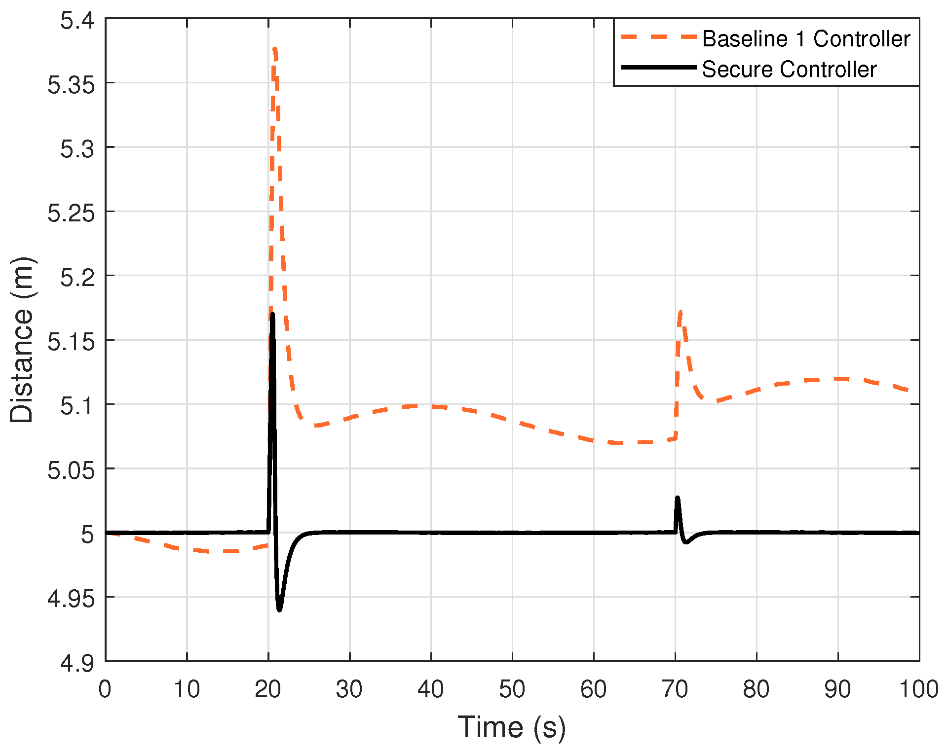
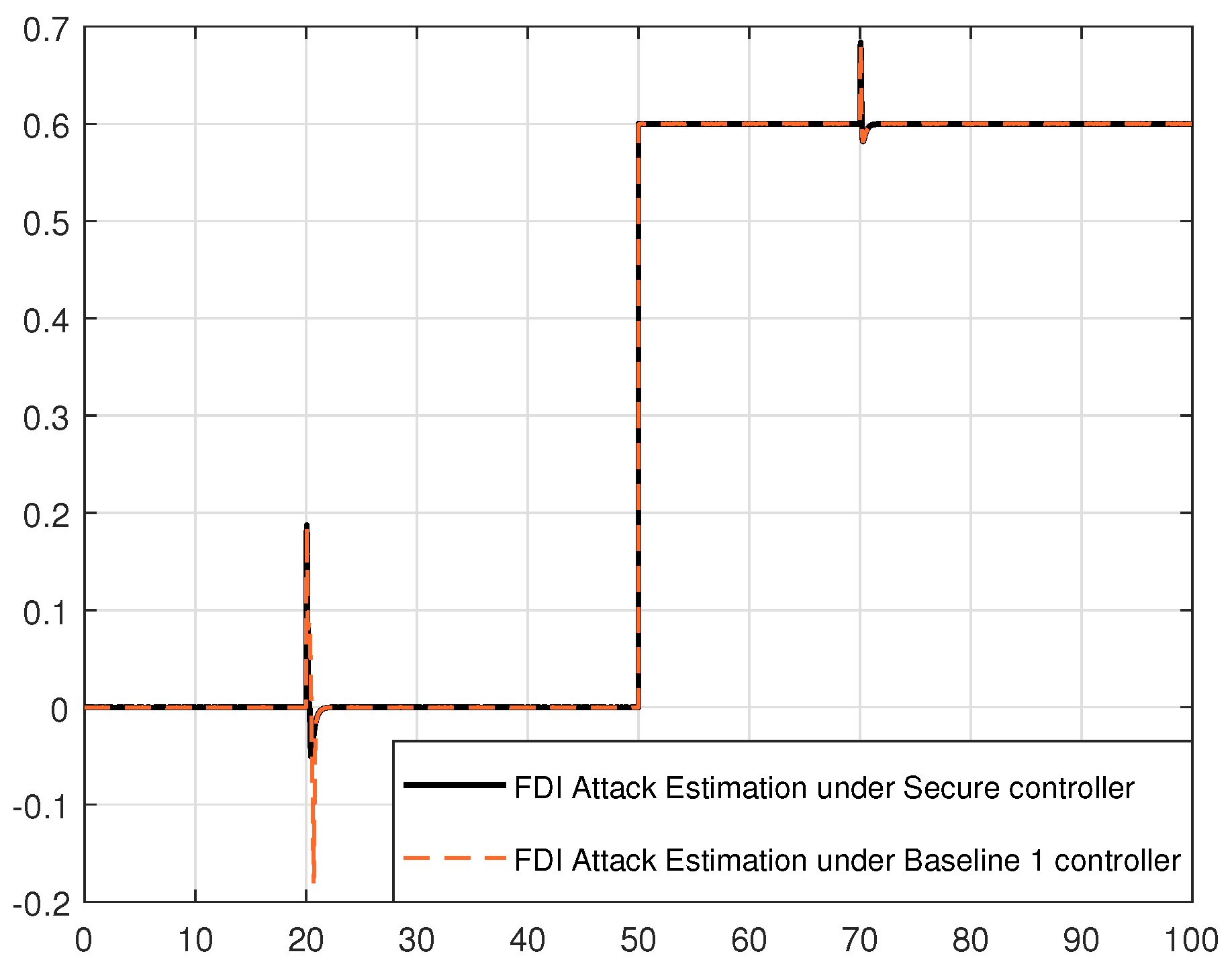
In this subsection, the effectiveness of the proposed secure controller is further validated by comparing its performance with the baseline 1 controller, as introduced in [22]. The control method presented in this paper incorporates an FDI attack estimator and employs a hybrid approach that integrates model-based and learning-based techniques. In addition, the controller design does not rely on the leader’s model. Figure 6 and Figure 7 illustrate that while the baseline 1 controller successfully maintains the desired distance and estimates the FDI attack, our proposed method demonstrates superior performance. To quantify this improvement,

Table 3. Root Mean Square Error of FDI attack estimation and distance between vehicles.

Paper	FDI Attack Estimation RMSE	Distance RMSE
Baseline 1 Controller	0.0097	0.0963
Proposed Controller	0.0056	0.0120

presents the RMSE values for distance and FDI attack estimation, providing a clear comparative assessment. Although the baseline 1 controller achieves low RMSE values, indicative of its good performance, our proposed controller exhibits even lower RMSE values, further confirming its enhanced accuracy and effectiveness.

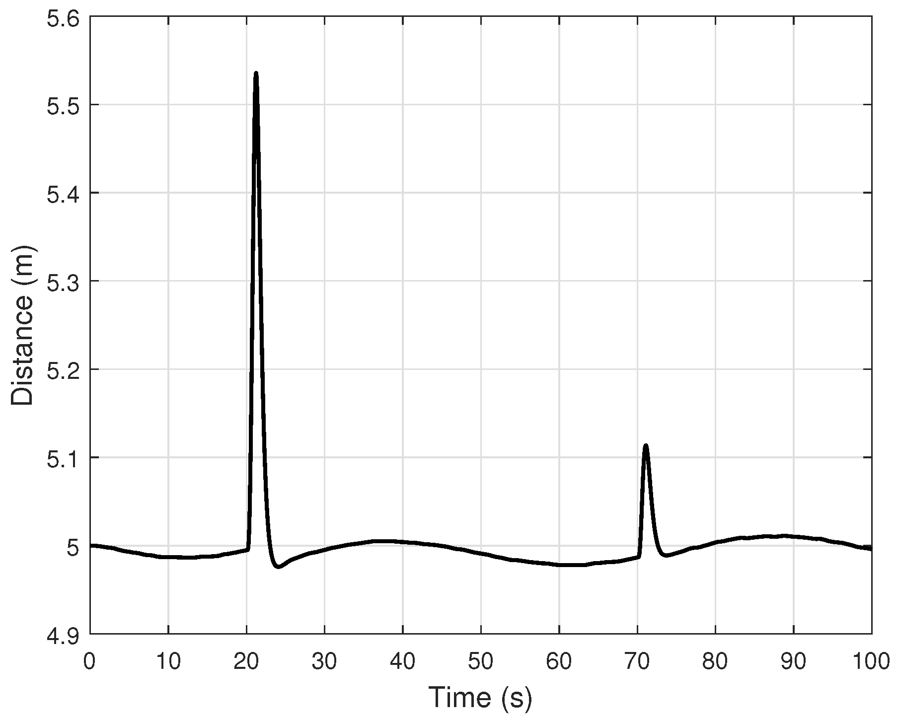
6.5. Platoon Scenario

In this subsection, we present an additional simulation involving a platoon of five vehicles, where the fourth vehicle is designated as the leader ($i-1$) and the fifth vehicle as the follower (i). In this scenario, an FDI attack is introduced as a step function with a step time of 50 s. The FDI attack function begins at an initial value of 0 and increases to a final value of 0.6, targeting the communication channels of all five vehicles. To further evaluate system robustness, we incorporated external disturbances modeled as $\zeta \sin (t/8)$ to the model of vehicles and a time-varying communication delay represented by ($\beta \left(2\sin \right(t/2)+3)$) into the transmitted control and velocity signals of the leader vehicle. Additionally, measurement noise was included in the Simulink model for a realistic evaluation. For the following figures, we used $\zeta =0.1$ and $\beta =0.01$. 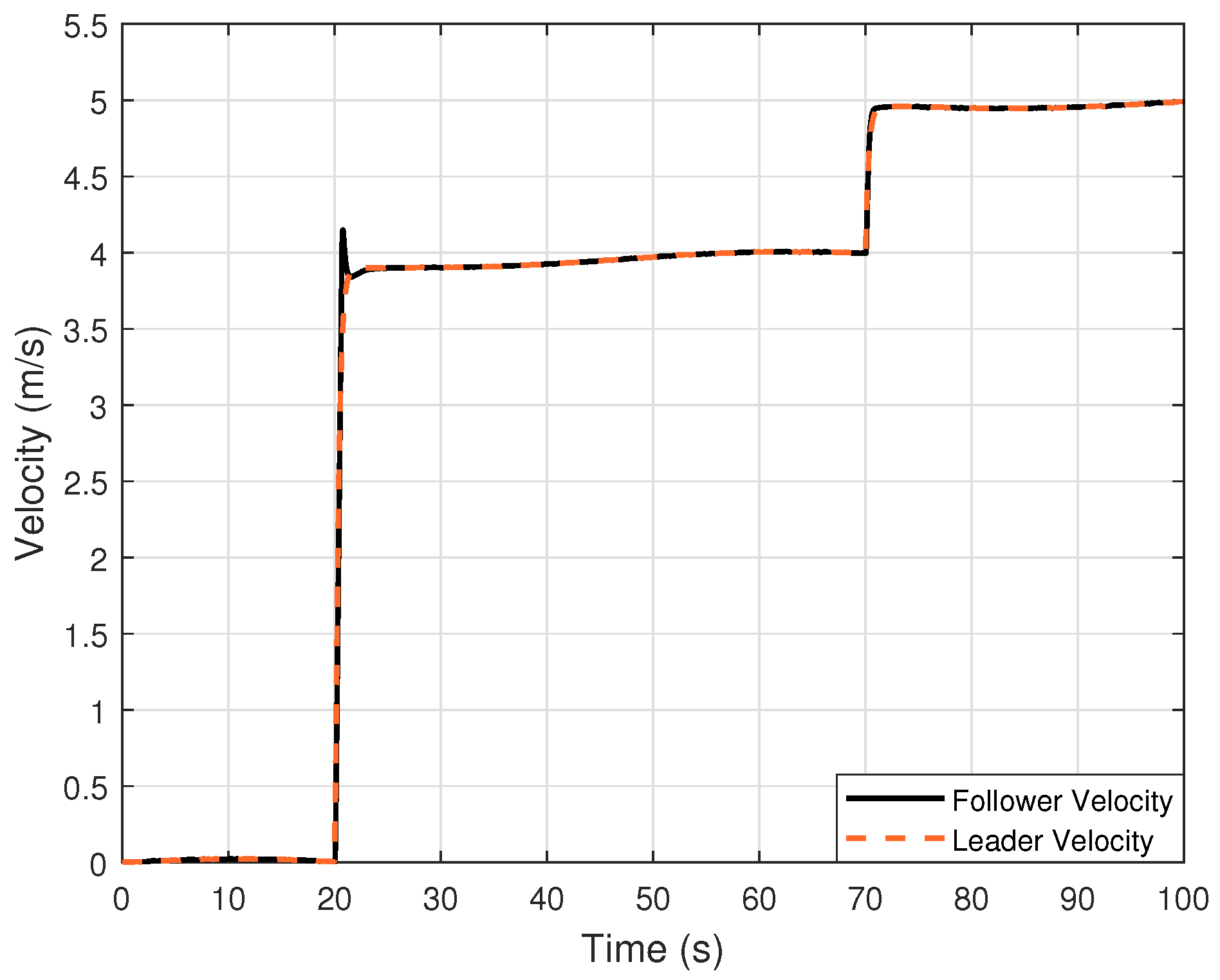As illustrated in Figure 8, the velocities of all five vehicles are depicted, demonstrating that even under the influence of FDI attack, external disturbances, measurement noise, and time-varying communication delays, the vehicles maintain harmonic movement, with each follower closely tracking its respective leader. 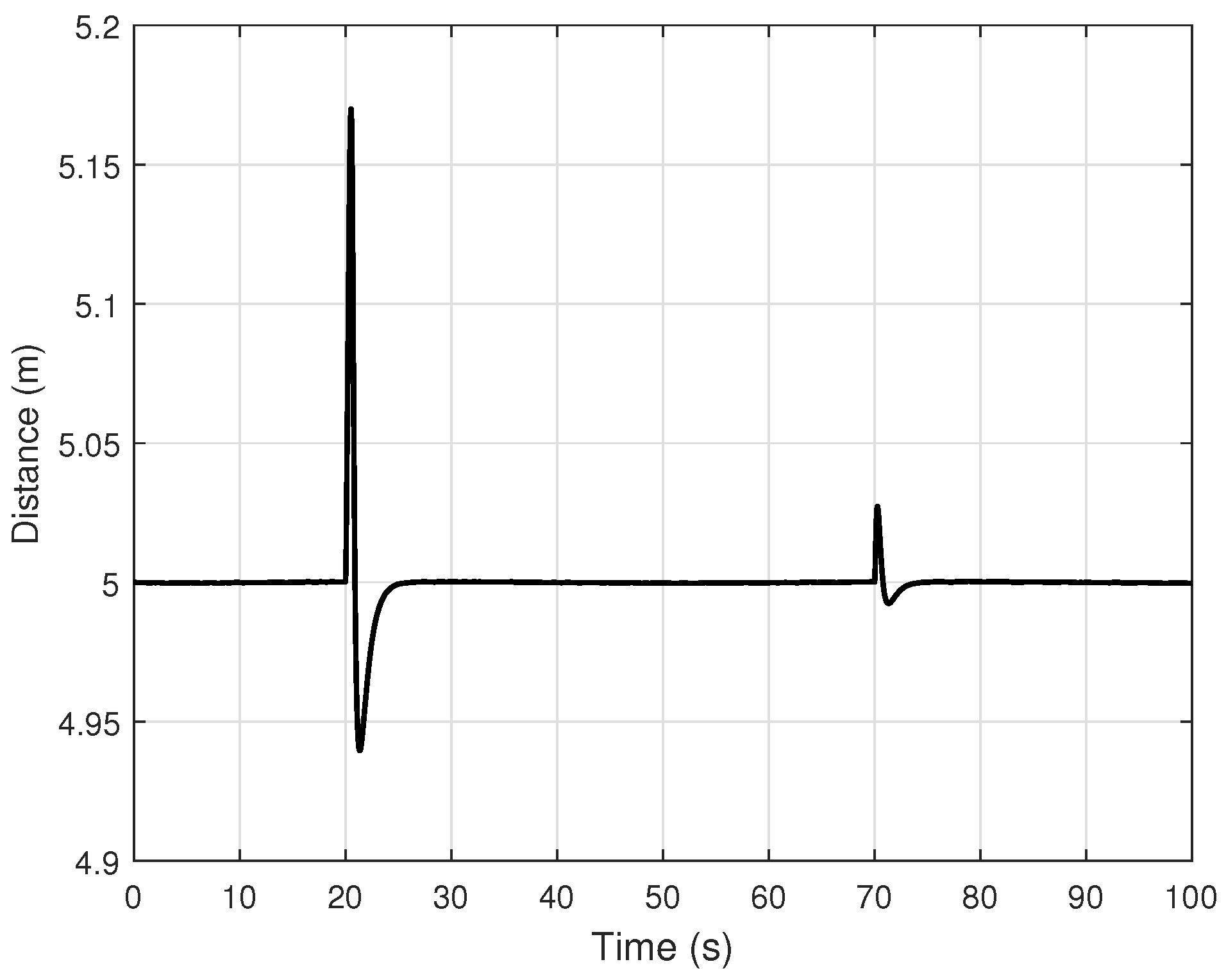Furthermore, Figure 9 shows the distance between the fourth and fifth vehicles. While minor deviations from the desired 5 m spacing are observed, the vehicles consistently maintain a safe inter-vehicle distance, significantly reducing the risk of collisions. To quantify the impact of disturbances and delays,

Table 4. Root Mean Square Error of distance between fourth and fifth vehicles for different values of disturbance and time delay.

Disturbance	Communication Time Delay	Distance RMSE Under Secure Controller
$0.1\sin (t/8)$	$0.01\left(2\sin \right(t/2)+3)$	0.0514
$0.2\sin (t/8)$	$0.02\left(2\sin \right(t/2)+3)$	0.0546
$0.3\sin (t/8)$	$0.03\left(2\sin \right(t/2)+3)$	0.0589

presents the RMSE value for inter-vehicle distance. The results clearly indicate that increasing the values of $\zeta$ and $\beta$ leads to higher RMSE values, reflecting the greater effects of larger disturbances and communication delays.

6.6. FDI Attacks on Control and Velocity Signals

In this subsection, we present a new scenario of the attacks on the communication between vehicles. A sophisticated attacker gains access to the communication channel and injects different types of FDI attacks into the transmitted data. Specifically, the velocity signal is disrupted by a uniform random disturbance signal, characterized by a minimum value of 0, a maximum value of 0.5, and a fixed seed of 1 to ensure repeatability. Concurrently, the control signal is subjected to two distinct step-function FDI attacks: the first initiates at 30 s, transitioning from an initial value of 0 to a final value of 0.3, while the second begins at 60 s with a similar transition from 0 to 0.3.

Additionally, the simulation includes a noise and a disturbance defined as $0.1\sin (t/8)$. As shown in Figure 10, the proposed method effectively mitigates the adverse effects of these diverse FDI attacks, disturbances, and measurement noise, ensuring that the desired safe distance between vehicles is maintained. Furthermore, Figure 11 illustrates how the following vehicle successfully tracks the leader vehicle, maintaining the same velocity profile despite the injected attacks and external disturbances. It is important to note that in this scenario, the estimation of FDI attacks is not performed when the injected attacks on the control and velocity signals are different. Our proposed method is designed to estimate FDI attacks effectively when the same attack is applied to both control and velocity signals.

6.7. Experimental Results

The experimental setup was designed to validate the results obtained from MATLAB Simulink by integrating the lead vehicle and controller within the Simulink environment while using the Ford Fusion as the follower vehicle. During testing, the control signal was generated within MATLAB Simulink and subsequently converted into a controller area network (CAN) message using dedicated Simulink blocks. This CAN message was then transmitted to the actual vehicle via CAN communication. The vehicle’s CAN bus interface facilitated both the reception and transmission of these messages. To establish seamless communication between Simulink on the computer and the vehicle’s CAN bus interface, Kvaser USB interfaces were employed. Once the control signal was received by the vehicle, its velocity data were extracted as CAN messages and sent back to MATLAB Simulink.

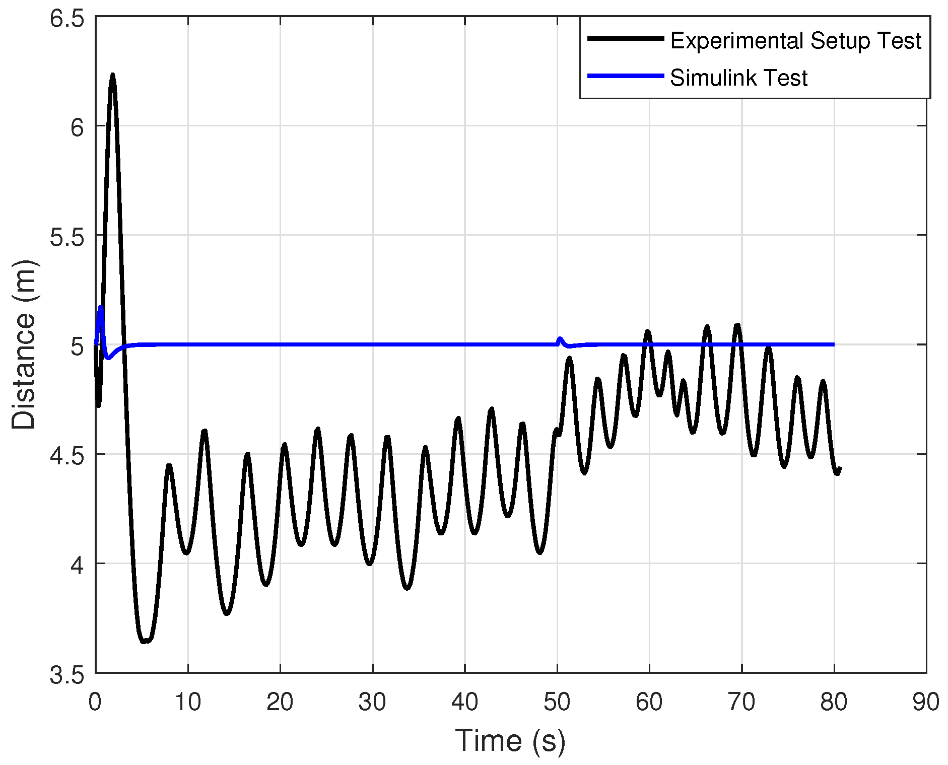
In this scenario, the FDI attack is modeled as a step function, starting at zero and increasing to 0.6 at 35 s. Additionally, a disturbance, represented as $0.1\sin (t/8)$, and measurement noise were introduced in the Simulink model to better simulate real-world conditions. The lead vehicle, initially positioned 10 m ahead of the follower, begins moving at the start of the test and increases its speed at the 50 s mark. Figure 12 shows the distance between the vehicles in both the Simulink simulation and the experimental setup. In the simulation, the desired inter-vehicle distance is well maintained throughout the test. In the experimental setup, some overshoots and undershoots appear when the lead vehicle changes its velocity. Despite these fluctuations, the minimum observed distance remains above 3.5 m, ensuring a low risk of collision. Figure 13 illustrates the velocity profile of the vehicles. As shown, the follower vehicle initially tries to match the movement of the leader, maintaining the 10 m gap. When the lead vehicle accelerates at 50 s, the follower responds accordingly. These results confirm that the follower successfully tracks the leader while maintaining a safe distance, demonstrating the effectiveness of the control strategy.

7. Conclusions and Future Work

7.1. Conclusions

CACC is a key feature of CAVs, enabling data collection from the leading vehicle and transmission to the following vehicle. To ensure the reliability of CACC, secure controllers should be designed to identify and mitigate FDI attacks. In this study, the leader’s control and velocity signals are subjected to FDI attacks. Additionally, discrepancies between the vehicle models, with the leader vehicle’s model being unknown, pose significant challenges. To counteract the effects of both FDI attacks and unknown leaders, a secure observer-based control system is designed. The proposed system accurately estimates FDI attacks and mitigates their effects, ensuring a safe following distance between vehicles. The effectiveness of the developed method was evaluated using MATLAB Simulink.

7.2. Future Work

While this study provides important insights into secure control for connected and autonomous vehicles, there are several exciting directions for future research. One possibility is exploring vehicle platooning in a multi-layer framework, where multiple platoons operate at different levels under varying traffic conditions. This could improve scalability and adaptability in real-world traffic scenarios. Additionally, instead of focusing only on the longitudinal dynamics of vehicles, future research could incorporate both longitudinal and lateral dynamics. This would offer a more realistic model of vehicle behavior, especially in situations involving lane changes, turns, and curved roads. Another important area for further investigation is the impact of real-world environmental factors on system performance. Conditions such as rain, snow, fog, road surface variations, and sensor noise could be studied to enhance the robustness of the control method.

References

1. Jia, D.; Lu, K.; Wang, J.; Zhang, X.; Shen, X. A survey on platoon-based vehicular cyber-physical systems. IEEE Commun. Surv. Tutor. 2015, 18, 263–284. [Google Scholar] [CrossRef]
2. Xiao, L.; Gao, F. A comprehensive review of the development of adaptive cruise control systems. Veh. Syst. Dyn. 2010, 48, 1167–1192. [Google Scholar] [CrossRef]
3. He, Y.; Ciuffo, B.; Zhou, Q.; Makridis, M.; Mattas, K.; Li, J.; Li, Z.; Yan, F.; Xu, H. Adaptive cruise control strategies implemented on experimental vehicles: A review. IFAC-PapersOnLine 2019, 52, 21–27. [Google Scholar] [CrossRef]
4. Kazemi, H.; Mahjoub, H.N.; Tahmasbi-Sarvestani, A.; Fallah, Y.P. A learning-based stochastic MPC design for cooperative adaptive cruise control to handle interfering vehicles. IEEE Trans. Intell. Veh. 2018, 3, 266–275. [Google Scholar] [CrossRef]
5. Wang, Z.; Wu, G.; Barth, M.J. A review on cooperative adaptive cruise control (CACC) systems: Architectures, controls, and applications. In Proceedings of the 2018 21st International Conference on Intelligent Transportation Systems (ITSC), Maui, HI, USA, 4–7 November 2018; IEEE: Piscataway, NJ, USA, 2018; pp. 2884–2891. [Google Scholar]
6. Bonab, P.A.; Sargolzaei, A. A Nonlinear Control Design for Cooperative Adaptive Cruise Control with Time-Varying Communication Delay. Electronics 2024, 13, 1875. [Google Scholar] [CrossRef]
7. Shladover, S.E. Connected and automated vehicle systems: Introduction and overview. J. Intell. Transp. Syst. 2018, 22, 190–200. [Google Scholar] [CrossRef]
8. Ploeg, J.; Scheepers, B.T.; Van Nunen, E.; Van de Wouw, N.; Nijmeijer, H. Design and experimental evaluation of cooperative adaptive cruise control. In Proceedings of the 2011 14th International IEEE Conference on Intelligent Transportation Systems (ITSC), Washington, DC, USA, 5–7 October 2011; IEEE: Piscataway, NJ, USA, 2011; pp. 260–265. [Google Scholar]
9. Bouadi, M.; Jiang, R.; Jia, B.; Zheng, S.T. String Stability Analysis of Cooperative Adaptive Cruise Control Vehicles Considering Multi-Anticipation and Communication Delay. IEEE Trans. Intell. Transp. Syst. 2024, 25, 11359–11369. [Google Scholar] [CrossRef]
10. Dey, K.C.; Yan, L.; Wang, X.; Wang, Y.; Shen, H.; Chowdhury, M.; Yu, L.; Qiu, C.; Soundararaj, V. A review of communication, driver characteristics, and controls aspects of cooperative adaptive cruise control (CACC). IEEE Trans. Intell. Transp. Syst. 2015, 17, 491–509. [Google Scholar] [CrossRef]
11. Rezaee, H.; Zhang, K.; Parisini, T.; Polycarpou, M.M. Cooperative adaptive cruise control in the presence of communication and radar stochastic data loss. IEEE Trans. Intell. Transp. Syst. 2024, 25, 4964–4976. [Google Scholar] [CrossRef]
12. Zhai, C.; Chen, C.; Zheng, X.; Han, Z.; Gao, Y.; Yan, C.; Luo, F.; Xu, J. Ecological cooperative adaptive cruise control for heterogenous vehicle platoons subject to time delays and input saturations. IEEE Trans. Intell. Transp. Syst. 2022, 24, 2862–2873. [Google Scholar] [CrossRef]
13. Pham, M.; Xiong, K. A survey on security attacks and defense techniques for connected and autonomous vehicles. Comput. Secur. 2021, 109, 102269. [Google Scholar] [CrossRef]
14. Suo, D.; Moore, J.; Boesch, M.; Post, K.; Sarma, S.E. Location-based schemes for mitigating cyber threats on connected and automated vehicles: A survey and design framework. IEEE Trans. Intell. Transp. Syst. 2020, 23, 2919–2937. [Google Scholar] [CrossRef]
15. Zhu, P.; Jin, S.; Bu, X.; Hou, Z. Distributed Data-Driven Control for a Connected Autonomous Vehicle Platoon Subjected to False Data Injection Attacks. IEEE Trans. Autom. Sci. Eng. 2023, 21, 7527–7538. [Google Scholar] [CrossRef]
16. Mirwald, J.; Ultsch, J.; de Castro, R.; Brembeck, J. Learning-Based Cooperative Adaptive Cruise Control. Actuators 2021, 10, 286. [Google Scholar] [CrossRef]
17. Stanger, T.; del Re, L. A model predictive cooperative adaptive cruise control approach. In Proceedings of the 2013 American Control Conference, Washington, DC, USA, 17–19 June 2013; IEEE: Piscataway, NJ, USA, 2013; pp. 1374–1379. [Google Scholar]
18. Wen, S.; Guo, G.; Chen, B.; Gao, X. Cooperative adaptive cruise control of vehicles using a resource-efficient communication mechanism. IEEE Trans. Intell. Veh. 2018, 4, 127–140. [Google Scholar] [CrossRef]
19. Kayacan, E. Multiobjective H control for string stability of cooperative adaptive cruise control systems. IEEE Trans. Intell. Veh. 2017, 2, 52–61. [Google Scholar] [CrossRef]
20. Biroon, R.A.; Biron, Z.A.; Pisu, P. False data injection attack in a platoon of CACC: Real-time detection and isolation with a PDE approach. IEEE Trans. Intell. Transp. Syst. 2021, 23, 8692–8703. [Google Scholar] [CrossRef]
21. Ansari-Bonab, P.; Holland, J.C.; Cunningham-Rush, J.; Noei, S.; Sargolzaei, A. Secure Control Design for Cooperative Adaptive Cruise Control Under False Data Injection Attack. IEEE Trans. Intell. Transp. Syst. 2024, 25, 9723–9732. [Google Scholar] [CrossRef]
22. Ansari Bonab, P.; Javidi-Niroumand, F.; Sargolzaei, A. Secure control design for cooperative adaptive cruise control with a time-varying input delays under false data injection attacks. Int. J. Syst. Sci. 2024, 56, 375–393. [Google Scholar] [CrossRef]
23. Patre, P.M.; MacKunis, W.; Kaiser, K.; Dixon, W.E. Asymptotic tracking for uncertain dynamic systems via a multilayer neural network feedforward and RISE feedback control structure. IEEE Trans. Autom. Control 2008, 53, 2180–2185. [Google Scholar] [CrossRef]
Figure 1. A string of heterogeneous vehicles with the CACC feature, under FDI attacks.
Computers 14 00084 g001
Figure 2. Proposed solution diagram.
Computers 14 00084 g002
Figure 3. FDI attack estimation, velocity profile of vehicles, and distance between vehicles for scenario 1.
Computers 14 00084 g003
Figure 4. FDI attack estimation, velocity profile of vehicles, and distance between vehicles for scenario 2.
Computers 14 00084 g004
Figure 5. FDI attack estimation, velocity profile of vehicles, and distance between vehicles for scenario 3.
Computers 14 00084 g005
Figure 6. Distance between lead and following vehicles for comparison scenario.
Computers 14 00084 g006
Figure 7. FDI attack estimation for comparison scenario.
Computers 14 00084 g007
Figure 8. Velocity profile of all vehicles in the platoon.
Computers 14 00084 g008
Figure 9. Distance between the fourth and fifth vehicles.
Computers 14 00084 g009
Figure 10. Distance between vehicles under two different FDI attacks.
Computers 14 00084 g010
Figure 11. Velocity profile of the following and lead vehicles under two different FDI attacks.
Computers 14 00084 g011
Figure 12. Distance between lead and following vehicles in experimental setup test.
Computers 14 00084 g012
Figure 13. Velocity profile of lead and following vehicles in experimental setup test.
Computers 14 00084 g013