Practice and Research Optimization Environment in Python (PyPROE)

Abstract

Practice and Research Optimization Environment in Python (PyPROE) is a GUI-based, integrated framework designed to improve the user experience in both learning and research on engineering design optimization. Traditional optimization programs require either coding or creating complex input files, and often involve a variety of applications in sequence to arrive at the solution, which presents a steep learning curve. PyPROE addresses these challenges by providing an intuitive, user-friendly Graphical User Interface (GUI) that integrates key steps in design optimization into a seamless workflow through a single application. This integration reduces the potential for user error, lowers the barriers to entry for learners, and allows students and researchers to focus on core concepts rather than software intricacies. PyPROE’s human-centered design simplifies the learning experience and enhances productivity by automating data transfers between function modules. This automation allows users to dedicate more time to solving engineering problems rather than dealing with disjointed tools. Benchmarking and user surveys demonstrate that PyPROE offers significant usability improvements, making complex engineering optimization accessible to a broader audience.

1. Introduction

Design optimization is crucial in many engineering fields such as mechanical, aerospace, and civil engineering. Traditional tools for optimization, especially in educational and research contexts, present significant challenges. Most optimization tools require users to code directly into solvers or construct complex input files, which can be intimidating for students and time-consuming for researchers. Additionally, integrating various functionalities like Design of Experiments (DOE), metamodeling, and optimization often requires switching between several software tools, resulting in cumbersome workflows and increased chances of user errors. These fragmented workflows create steep learning curves for undergraduate students, graduate students, and researchers who often do not have extensive programming skills. Practice and Research Optimization Environment in Python (PyPROE) was conceived to address these challenges within the framework of Human–Computer Interaction (HCI), which considers psychology as a science of design [1]. PyPROE is a user-centric, Python-based framework integrating DOE, metamodeling, and optimization into a unified, intuitive environment. PyPROE simplifies the HCI process of stimulus identification and response selection by prioritizing ease of use through an interactive Graphical User Interface (GUI) to minimize human error and eliminate the need for switching between various software tools, making optimization accessible to both beginners and advanced users [2].

1.1. Human–Computer Interaction

HCI is a multidisciplinary field that focuses on improving user experience through intelligent design and intuitive, efficient, and accessible software development [3]. In this context, HCI emphasizes creating interfaces that are easy to use and meet the objective(s) of the software itself by understanding user behavior. For ease of use, HCI principles advocate for clean and minimalistic design, logical navigation, and fewer steps to complete tasks [4,5]. This often includes intuitive icons, clear labels, and consistent layouts. Usability testing is critical to HCI to help designers refine software based on user feedback, eliminate pain points, and enhance accessibility [6]. All-in-one methodologies in HCI aim to streamline multiple functions into a single interface, reducing the need for users to switch between tools or platforms [7]. This integration improves productivity by minimizing disruptions and offering a cohesive experience. All-in-one solutions are designed around the idea that users can access all needed information and functionalities within a single system, thereby saving time and reducing the learning curve [3]. In practice, this requires careful planning of information architecture, prioritizing core functions, and ensuring that adding new features does not complicate users’ experience.

1.2. Engineering Design Optimization Methodologies

Design optimization has been used in various engineering disciplines [8,9,10,11]. Design optimization for engineering applications often involves detailed setup due to the complexity of the designs. This requires understanding the design constraints and creating the response surfaces of the objective and constraint functions that are often unavailable in explicit mathematical forms. 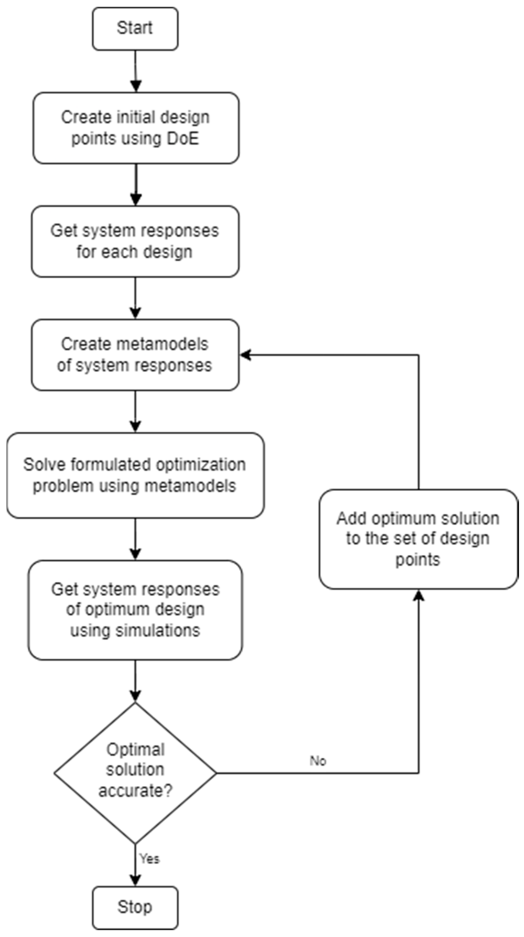In these situations, engineers rely on metamodeling to create approximate functions using function values of the objective(s) and constraints obtained with numerical or experimental tools [12,13,14]. The metamodels are then used in optimization and can be iteratively updated/improved using the optimum designs based on the previous metamodels. This process, as illustrated in Figure 1, continues until the optimum solution (determined by the tolerances set in the iterative process) is found to have sufficient accuracy determined by the true function values.

1.3. Design Optimization Workflows

All the functionalities in the design optimization workflow, as illustrated in Figure 1, were implemented in PyPROE, except for “getting system responses”, which is application/problem-specific and depends on external simulation tools.

Table 1. Comparison of PyPROE with previous tools used in simulation-based design optimization.

Design Optimization Workflow	PyPROE	Previous Tools
Create initial design	Yes	HiPPO/Excel
Obtain system responses	By external simulation tools (problem-specific)
Create metamodels	Yes	HiPPO
Formulate problem	Yes	Notepad
Obtain gradients if necessary	Yes	Manual Derivation/Matlab
Create input file	Yes	Notepad
Solve formulated problem	Yes	GimOPT
Plot to visualize	Yes	Matlab
Update DOE	Yes	Excel/Notepad

shows a comparison of PyPROE with the previous tools used in simulation-based design optimization. It can be seen that there were many manual data transfers among multiple external programs using the previous tools, and that they were all eliminated in PyPROE, resulting in an increased speed of the workflow and eliminating potential human errors in data transfer and problem formulation.

2. PyPROE User Interface and Functionality

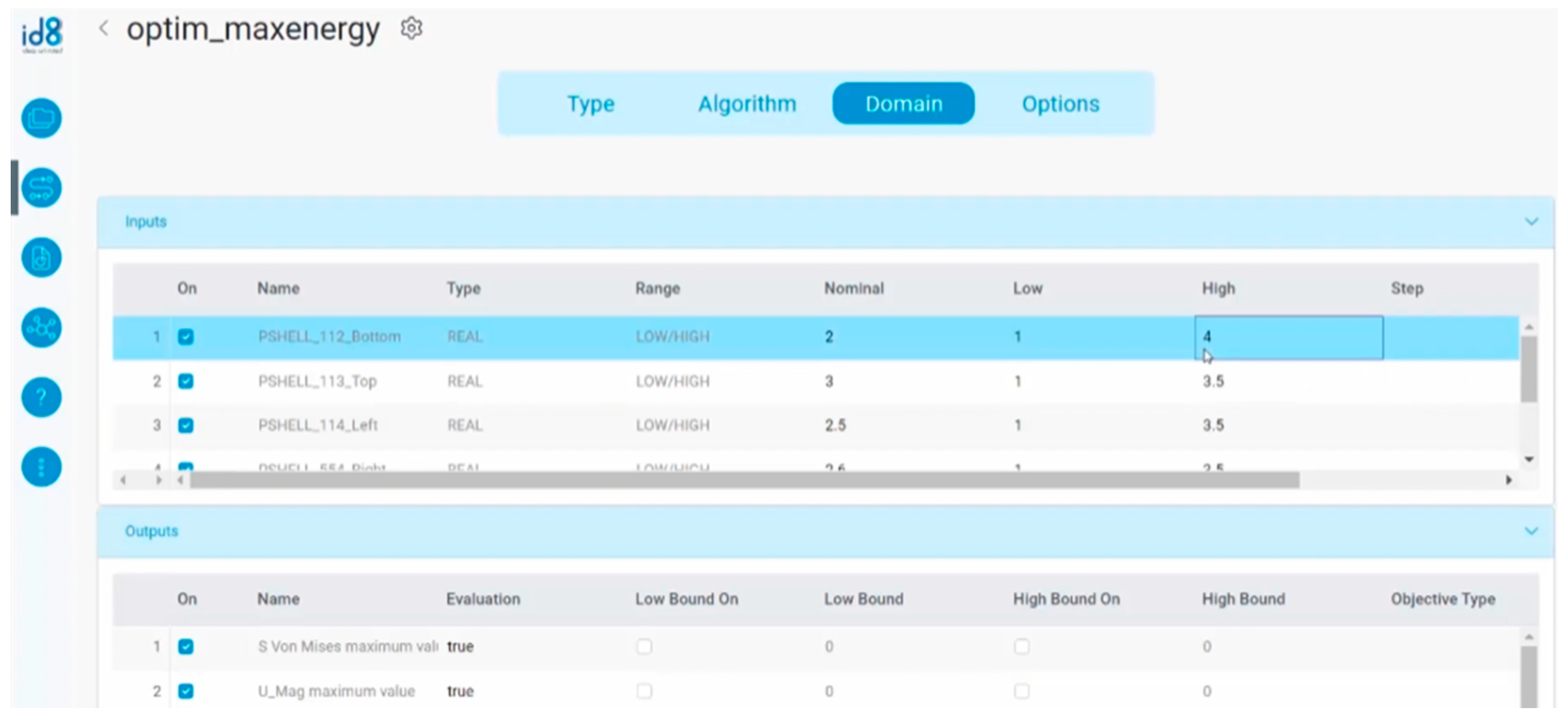
Previous generations of design optimization tools required the use of command line arguments and/or extensive coding language requirements, along with other interface inefficiencies such as manual data transferring between different tools. While some commercial tools offer streamlined user interfaces, as shown by the example in Figure 2, they require costly licenses and are not as easily extended as those built with existing industry standard libraries. In the case of NEOSIS [15], to the best of the authors’ knowledge, it lacks features such as sensitivity analysis and automatic symbolic gradient calculation that are useful for design optimization. Although commonly used engineering tools such as Matlab and MathCAD [16,17] have optimization capabilities and some extended features such as symbolic differentiation, they often require significant coding for any given design optimization problem. While the previous software tools (GimOPT and HiPPO) eliminated the need for coding, they require manual data transfer and lack a user-friendly interface. PyPROE was developed to overcome these drawbacks while maintaining and integrating all functionalities in one software tool.

To demonstrate the use of PyPROE in the optimization workflow, a single-objective optimization problem (see Figure 2) is adopted to design a cantilever beam with minimum weight, no more than 5 mm of maximum deflection, and no more than 250 MPa of the maximum principal stress.

The standard formulation of the design optimization problem is as follows:

$$\begin{array}{ll}\mathrm{Min}.& M=\rho LA\\ \mathrm{s}.\mathrm{t}.& {\Delta }_{Max}-0.005\le 0\\ & {\sigma }_{Max}-250\times {10}^6\le 0\\ & 0.020\le d\le 0.060\\ & 0.002\le t\le 0.008\end{array}$$

(1)

where $d$ and t are the two design variables representing the diameter and thickness of the beam, respectively, $\rho$ is the density, L is the length, and $A$ is the cross-sectional area of the beam. In Equation (1), the objective function, M, is the mass of the beam, and the two constraint functions, ${\Delta }_{Max}$ and ${\mathsf{\sigma }}_{Max}$, are the maximum deflection and the maximum principal stress of the beam, respectively. The two constraint functions and the cross-sectional area are calculated by

$${\Delta }_{Max}={\displaystyle \frac{P{L}^3}{3EI}}$$

(2)

$${\sigma }_{Max}={\displaystyle \frac{PL\frac{d}{2}}{I}}={\displaystyle \frac{PLd}{2I}}$$

(3)

$$A={\displaystyle \frac{\pi \left[d^2-(d-2t{)}^2\right]}{4}}$$

(4)

where $I$ is the second moment of the area given by

$$I={\displaystyle \frac{\pi \left[d^4-(d-2t{)}^4\right]}{64}}$$

(5)

Note that in this example, Equations (2) and (3) were used in lieu of the external simulation tool(s) to calculate the system responses, i.e., the deflection and stress corresponding to each design. For more complicated engineering applications, these system responses are typically obtained using numerical simulation tools in which case metamodeling is needed to create explicit mathematical functions of these system responses.

PyPROE’s interface was designed following the HCI principles. For example, the decision to use large buttons for main actions was to improve visibility, and the automatic internal data transfer from one function tab to another was to eliminate human errors that occurred during manual data transfer using previous software tools. The inclusion of tool tips on many parts of PyPROE stemmed from the affordance principle of HCI. The main HCI principle, learnability, was considered for the whole system such that students could learn most of the functionalities of the software tool with a minimum amount of tutoring.

2.1. Design of Experiments

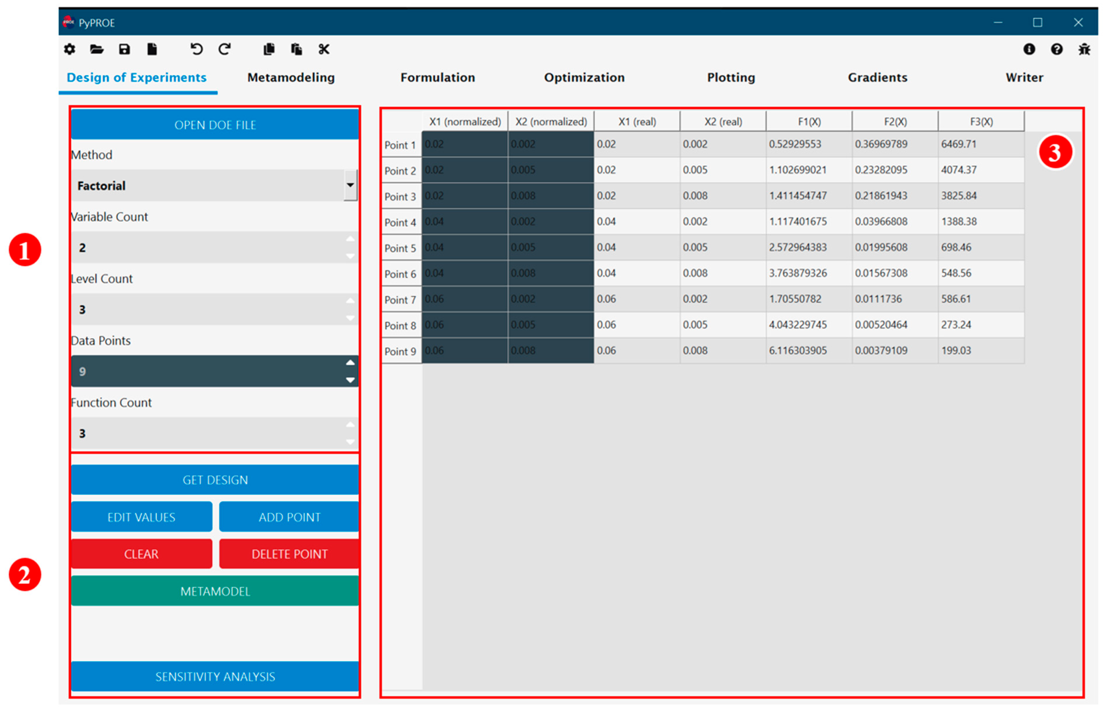
Design of Experiments is the first step in simulation-based optimization when metamodels need to be created for functions without explicit mathematical forms. Under PyPROE’s DOE tab, the user chooses the DOE method and defines the number of design variables, design levels, and functions for which metamodels are to be created. In the case of the cantilever beam design problem, the three-level factorial design method is chosen with two variables and three functions. In the design matrix shown in Figure 3, the function values are either obtained using external simulations and entered as numerical values or calculated using user-defined functions (as is the case here) similar to an Excel spreadsheet. This design matrix is automatically kept by PyPROE and sent to the next step, metamodeling, with a click on the button “Metamodel”.

2.2. Metamodeling

The Metamodeling tab, shown in Figure 4, provides easy generation of metamodels either using the design matrix from the DOE tab or loading in a previously generated DOE file. The generated metamodel functions, along with their gradient functions, are kept and can be sent to the formulation tab with an easy mouse click.

The metamodeling options in PyPROE include polynomial regression and Radial Basis Functions (RBFs). Polynomial regression can produce metamodels using linear polynomials, quadratic polynomials without interactions, or quadratic polynomials with paired interactions. These metamodels are simple but lack the ability to capture highly nonlinear responses. RBF metamodels, which are complicated and capable of capturing both low-order and highly nonlinear responses, are included in PyPROE with both traditional and new basis functions.

2.3. Formulation

The formulation tab allows the user to create optimization problems using the variables and user-defined functions and/or metamodels. As shown in Figure 5, the drop-down menus allow the user to quickly assign objective and constraint functions and define/edit appropriate variable ranges. Additionally, functions can also be loaded from files of previously generated PyPROE functions or other user-created functions.

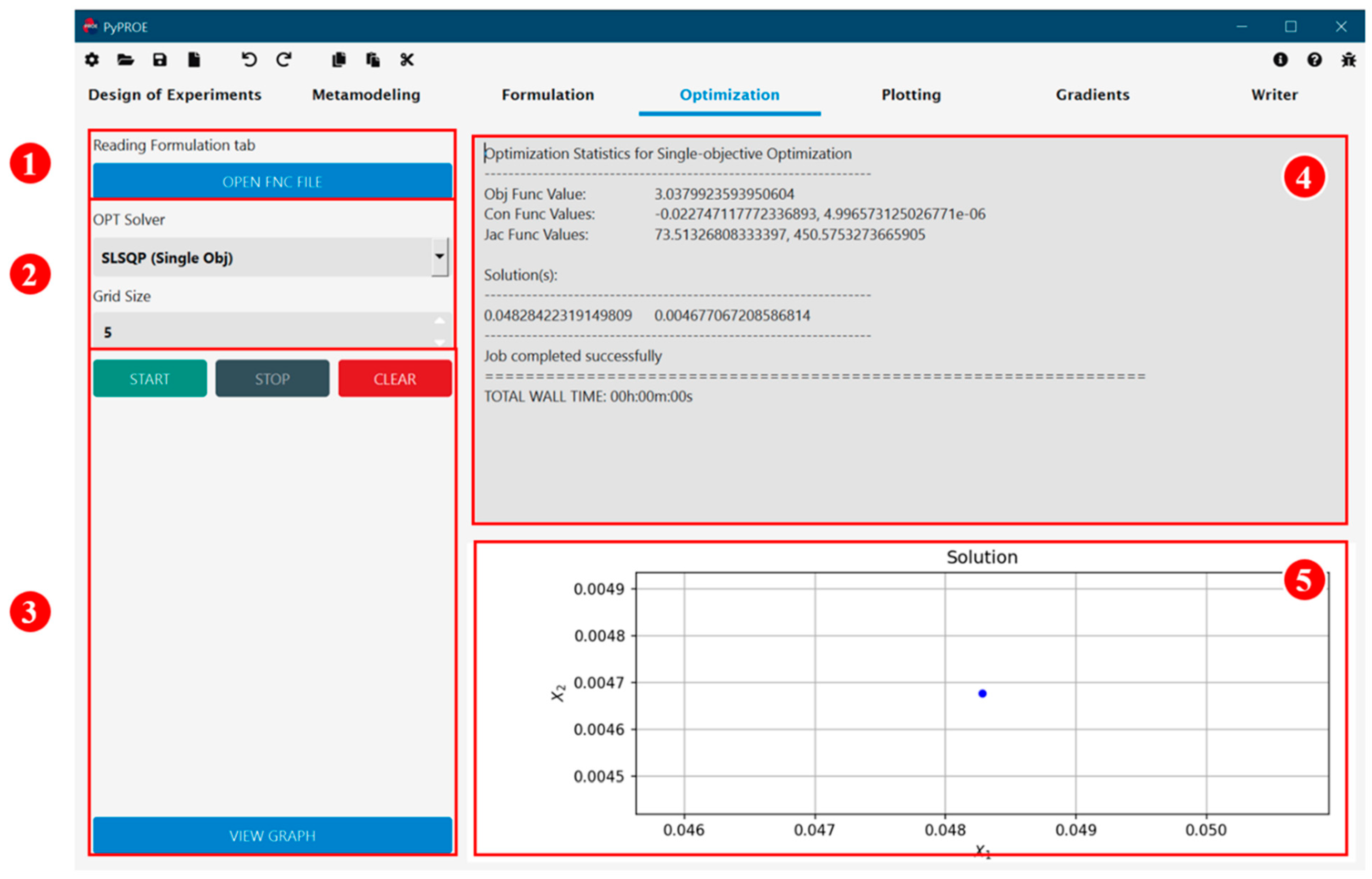
2.4. Optimization

The Optimization tab provides users with a selection of optimization solvers/algorithms: Sequential Least SQuare Programming (SLSQP), SLSQP with weighted sum formulation, Nondominated Sorting Genetic Algorithm (NSGA) second generation (NSGA-II) and third generation (NSGA-III), and Epsilon Multi-Objective Evolutionary Algorithm (EpsMOEA) [18]. In PyPROE, the optimization problem can be loaded from a previously generated and saved input file or directly from the formulation tab. Figure 6 shows the user interface of the PyPROE for the cantilever beam problem. The SLSQP solver was selected, and the optimum solution was promptly obtained and displayed along with the graph representation. Note that the generated graph can be displayed in a pop-up window for detailed inspection if desired.

2.5. PyPROE Supporting Features

Prior to applying optimization algorithms to a problem, PyPROE allows users to view the response functions or calculate the gradients of functions without user-supplied gradient functions. Previously, students had to use third-party software such as MATLAB for visualizations before proceeding with the optimization process. Additionally, if their objective and/or constraint functions did not have gradient functions, the students would be required to use either other software or hand calculation to obtain the gradients and put them into the input file for optimization.

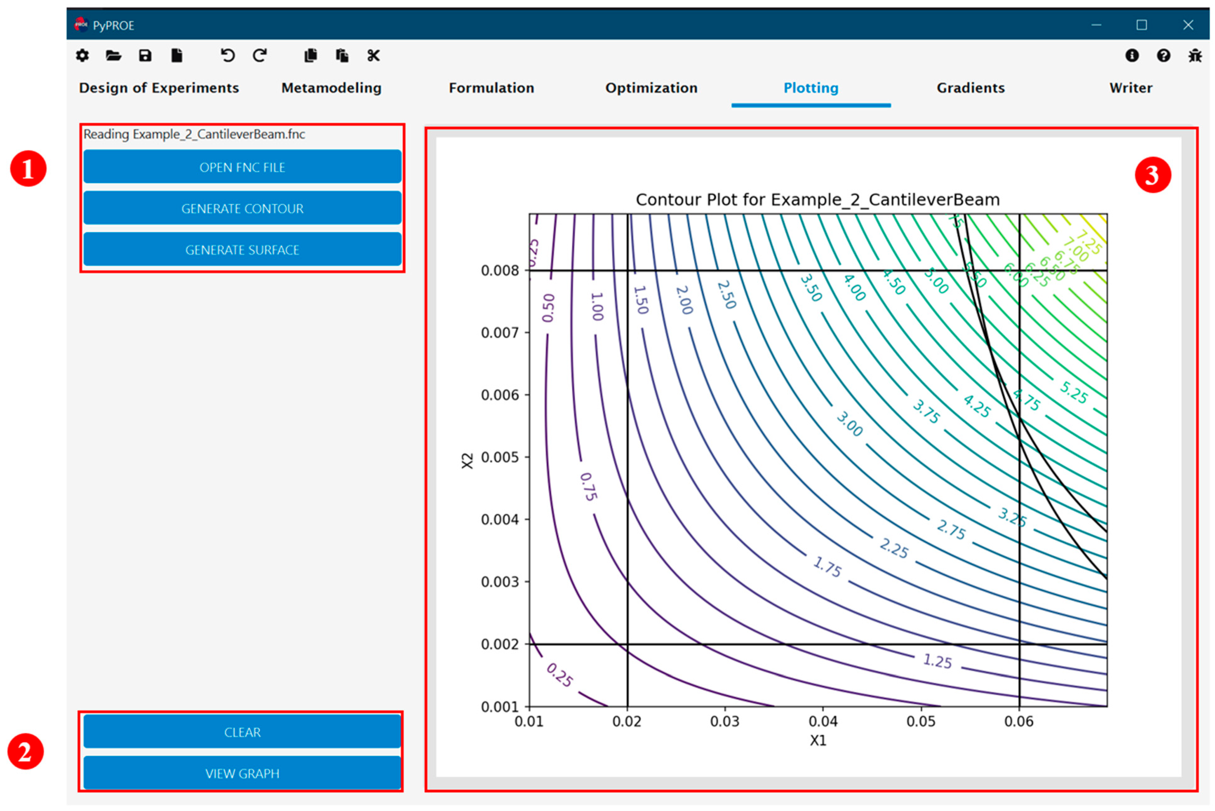
Figure 7 shows PyPROE’s Plotting tab that allows the user to open a previously saved function file and generate contours or surface plots of the functions. The graph can also be displayed in a separate window for further manipulation such as editing properties like labels, adjusting the view dimensions of the graphs, and exporting the graph as an image.

The Gradient tab in Figure 8 also allows for importing functions from previously saved files and generates gradient functions using symbolic differentiation. This results in a clean and complete file primed for optimization, particularly where gradient-based methods require the generated partial differential equations with respect to each variable.

3. User Experience

Performing design optimization with the previous tools required multiple separate programs: the metamodeling program, HiPPO [19], the optimization solver, GimOPT [20], Excel, Notepad editor, and MATLAB. Students reported that the GUI of the HiPPO program was non-intuitive, and the command-line program, GimOPT, was archaic. While the software functionality was unaffected, this detracted the students from learning the concepts and added unnecessary time complexity to the process. Each step that required data to be manually passed from one program to the other also introduced extra possibilities for unintentional errors, resulting in extra time and effort in analyzing and correcting data transfer inputs.

3.1. User Experience with Previous Tools

Figure 9 shows the optimization workflow of solving the cantilever beam design problem with the previous tools. In this process, the user would first generate a normalized DoE matrix with HiPPO. The resulting DOE table needs to be copied into a spreadsheet, and the real variable values are calculated from the limits for each variable and their normalized values. This DOE table with real variable values is then formatted into a HiPPO input file and loaded into HiPPO’s Metamodeling tab. Once the metamodels are generated in HiPPO, the user is required to save these metamodel functions and manually generate an input file in which the optimization formulation is created. In this optimization input file, all variable data, metamodel functions, and gradients of all functions need to be provided. Finally, the GimOPT program is run in a command-line console and the input file is provided by the user along with other command-line parameters. The optimization results are saved in an output file where the user needs to manually extract data and use other software packages for post-processing and/or graphing (e.g., Excel spreadsheet, MATLAB). With adaptive metamodeling, which iterates the above process until a satisfactory solution is obtained and shown in Figure 10, the user’s workload is greatly increased, and this is also true for the likelihood of potential human errors.

3.2. User Experience with PyPROE

Upon completion of PyPROE, a user-experience study was conducted with 14 students who had used the previous software packages in their design optimization course. The students were given a pre-survey prior to using PyPROE to verify the participants’ familiarity with previous optimization tools and their usage of the tools outside of a class environment. A 15 min session was then given to each student to use PyPROE on several optimization problems (with provided DOE and other input files) without any knowledge or training regarding this software. Upon completion of the 15 min session, the students were shown a brief tutorial video of PyPROE, showing its various features. Afterward, a second 15 min session was given to the students to continue working on the assigned problems. Lastly, the students were given a post-survey on their experience with using PyPROE. The results of both surveys are summarized in

Table 2. Survey results of user experience on PyPROE and previous tools.

Primary Survey Questions	Average Score of Previous Tools	Average Score of PyPROE	Difference	Standard Deviation	t-Statistic
On a scale of 1 (poor) to 10 (excellent), rate the Design of Experiments functionality for completing assignments or personal work.	5.5	9.14	3.64	2.02	6.74
On a scale of 1 (poor) to 10 (excellent), rate the Metamodeling functionality for completing assignments or personal work.	5.71	9.14	3.43	1.87	6.86
On a scale of 1 (poor) to 10 (excellent), rate the Formulation functionality for completing the provided tasks.	5.5	9.29	3.79	1.76	8.04
On a scale of 1 (poor) to 10 (excellent), rate the Optimization functionality for completing the provided tasks?	5.5	9.43	3.93	1.73	8.49

. As indicated by the t-statistic, which has a critical value of 3.01 for a 99% confidence interval, there is a significant difference between user experiences on the previous tools and PyPROE. The total of 14 participants represents a large number of students who are still accessible and have used the previous software recently to provide accurate responses to the survey. For usability testing and evaluation, these samples are sufficient to show significant statistical differences [21,22,23,24].

The pre-survey showed that most participants had a moderately positive experience with the previous optimization tools, i.e., HiPPO and GimOPT, with an average score of 5.55 out of 10 on usability across the two pieces of software. Several participants expressed mild frustration with using multiple different applications, stating that it complicated and delayed the design optimization process. The post-survey yielded very positive responses from participants on PyPROE: the usability of all the functionalities including DOE, metamodeling, formulation, and optimization was rated an average of 9.25 out of 10. Participants described the interfaces as straightforward, intuitive, with a simple workflow, and tailored to fit specific needs. All the participants expressed a strong interest in using PyPROE for future classes and research efforts.

It is worth mentioning that during the first 15 min session on PyPROE, twelve of the fourteen participants finished the entire instruction set before the 12 min mark. Five of the fourteen participants ran into an issue with a part of the instructions, but they could self-diagnose the errors and retract the steps without guidance. The only major issue that appeared during this stage of testing was the difference in app layout experienced by one user who was accustomed to a Mac interface. The testing device was a Windows machine, and the small file icon in the upper left corner of the screen was not an intuitive button for the Windows-oblivious tester. As the software was initially designed with Windows users in mind, this will be added to considerations for future versions of PyPROE.

3.3. Comparison of Existing Tools

PyPROE offers a large benefit to students and researchers for its ease of use compared to previous tools such as GimOPT and HiPPO. Commonly used software tools available to engineering students and researchers for design optimization, such as Matlab and MathCAD, have incredible complexity when it comes to implementing design optimization. Other commercial tools such as NEOSIS require costly licenses and are typically unavailable to students and researchers. Since PyPROE takes advantage of standardized libraries and provides a seamless GUI, it greatly enhances usability and accessibility. However, the use of interpretive language, Python, and standard libraries also increases the overhead and makes it less computationally efficient than previous tools (GimOPT and HiPPO).

Table 3. Comparison of computational efficiency, ease of use, and cost of different software tools.

Software	Computational Efficiency	Ease of Use	Cost
GimOPT	High	Low	Free
HiPPO	High	Medium	Free
Matlab	High	Low	Medium
MathCAD	High	Low	Medium
NEOSIS id8	Medium	Medium	High
PyPROE	Medium	High	Free

shows a comparison of PyPROE with existing software tools for design optimization.

4. PyPROE for Multi-Objective Optimization

PyPROE was evaluated using several benchmark problems of multi-objective optimization on its solution quality compared to other optimization tools. The two benchmark problems shown in this paper were the Fonseca–Fleming and Kursawe problems, each presenting its own unique challenges to design optimization algorithms. The Fonseca–Fleming problem is characterized by a concave Pareto Front and the Kursawe problem combines a non-convex, discontinuous Pareto Front to test an algorithm’s ability to obtain solution points that would represent the entire Pareto Front well.

The use of SLSQP, first introduced by Kraft in 1988, and later added to SciPy in 2020, allows PyPROE to utilize an existing library for accurate gradient-based calculations [25,26].

Although PyPROE also provides the weighted sum formulation (WSF) methodology in tandem with SLSQP [25,26] for gradient-based MOO, it has documented poor performance on problems with concave Pareto Fronts [27]. Consequently, the benchmarking was performed with only the non-gradient-based algorithms: NSGA-II, NSGA-III, and Eps-MOEA. While similar in nature, each algorithm tackles the same problem with slightly different implementations and provides a user with configurable parameters to adjust the algorithm’s performance based on the nature of the problem at hand. These non-gradient-based methods use Platypus as their underlying library [18], which allows the students to call these methods from PyPROE’s GUI without the need to know any of the underlying codes.

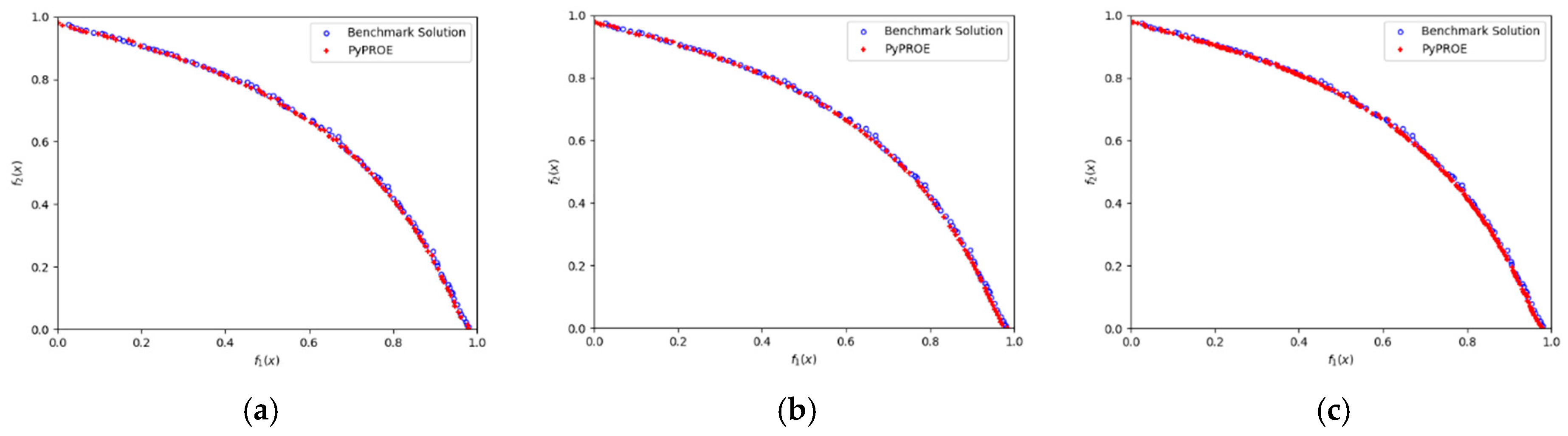
4.1. Fonseca–Fleming Problem

The Fonseca–Fleming problem is a two-objective, unconstrained optimization problem with the solutions forming a concave but continuous Pareto Front. This problem is formulated as follows:

$$\begin{gathered} \mathrm{Min}.\left\{\begin{array}{c}{f}_1\left(x\right)=1-e\left[-{\sum }_{i=1}^n{\left(x_i-{\displaystyle \frac{1}{\sqrt{n}}}\right)}^2\right]\\ f_2\left(x\right)=1-e\left[-{\sum }_{i=1}^n{\left(x_i+{\displaystyle \frac{1}{\sqrt{n}}}\right)}^2\right]\end{array}\right. \\ -5\le x_i\le 5 \\ 1\le i\le 3 \end{gathered}$$

(6)

The three evolutional algorithms implemented in PyPROE were used to solve this problem, and the results are highlighted in Figure 11, along with the benchmark solutions of the true Pareto Front. It can be seen that solutions from PyPROE’s two NSGA algorithms and Eps-MOEA represented the Pareto Front well and had good accuracy, with solutions closely matching the benchmark solutions.

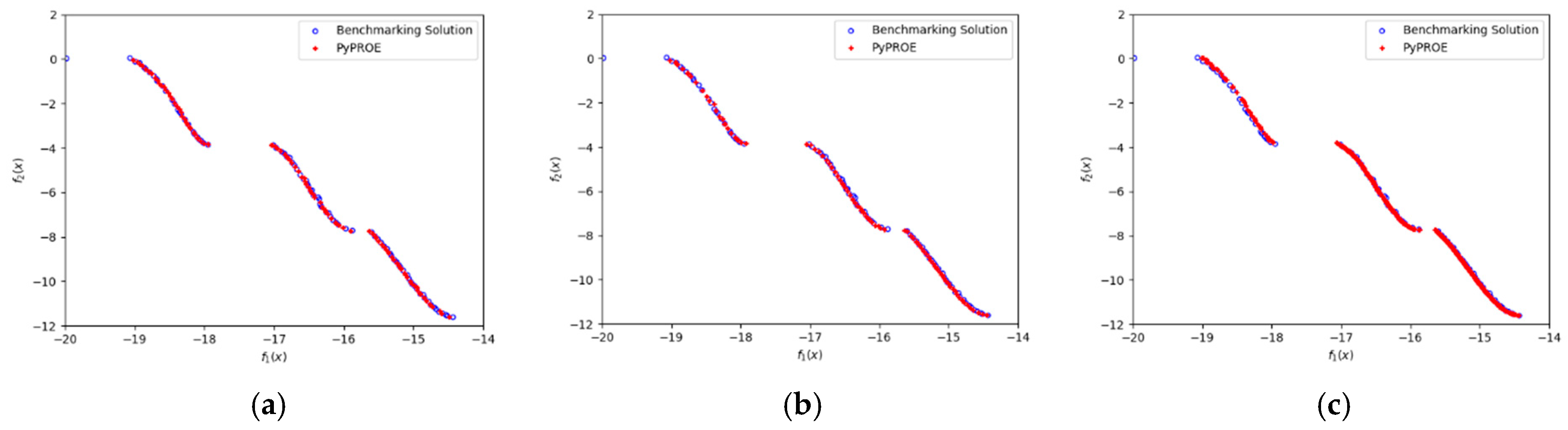
4.2. Kursawe Problem

The Kursawe problem is a two-objective, unconstrained optimization problem with a discontinuous Pareto Front. To obtain good solutions for this problem, optimization algorithms must show their ability to explore the design space effectively. The formulation of this problem is as follows:

$$\begin{array}{cc}\hfill \mathrm{Min}.& \left\{\begin{array}{c}{f}_1\left(x\right)=\sum _{i=1}^2\left[-10e\left(-0.2\sqrt{x_i^2}+x_{i+1}^2\right)\right]\\ f_2\left(x\right)=\sum _{i=1}^3\left[{\left|x_i\right|}^{0.8}+5\sin \left(x_i^3\right)\right]\end{array}\right.\hfill \\ & -5\le x_i\le 5\hfill \\ & 1\le i\le 3\hfill \end{array}$$

(7)

It can be seen from the results in Figure 12 that all three algorithms effectively capture the shape of the Pareto Front and achieve even distributions of the solution points on the Pareto Front.

The results in Figure 11 and Figure 12 demonstrate the effectiveness of PyPROE in solving multi-objective optimization problems, including the challenging problems chosen for this paper. While PyPROE’s GUI makes it easy to further explore optimum solutions by changing algorithm-specific parameters, the architecture of PyPROE also allows for ease of implementation and the addition of other optimization algorithms.

5. Conclusions

The development of PyPROE successfully addresses the challenges inherent in traditional optimization tools by providing an integrated, intuitive, and GUI-based framework for engineering design optimization. By combining different functionalities such as Design of Experiments, metamodeling, and optimization within a unified environment, PyPROE reduces the time and effort of both new and experienced users, greatly enhances the efficiencies, and minimizes potential human errors associated with data transfers among multiple software tools. This makes optimization methodologies more accessible to undergraduate and graduate students and other researchers, significantly enhancing their ability to experiment, learn, and innovate. The major drawback of PyPROE lies in its lower computational efficiency due to the use of Python and its libraries than the previous tool using C++. Future development of PyPROE may include evaluating and adopting libraries to improve its computational efficiency.

PyPROE’s intuitive user interface, designed by following modern HCI principles, delivers a smooth user experience and encourages engagement with complex engineering tasks. Survey results from students who used the previous optimization tools validated PyPROE’s enhanced user experience, which provides an easy connection between theoretical knowledge and practical application through the streamlined workflows. The accuracy of PyPROE’s solutions, validated against challenging benchmark problems, confirms the reliability of the software. Testing will continue with the subsequent iterations of the design optimization class. With good accuracy and large steps in quality-of-life features for the students, PyPROE enables students to spend less time remembering disjointed workflows and instead engage with the content smoothly and learning-centric.

6. Future Work

PyPROE was made with a purposefully limited scope, and one of the limitations was to make it compatible with the design optimization course. In the future, the software program will be extended with additional functionality to facilitate research in design optimization. One key point of future work is to exchange Platypus for pymoo, as the latter provides better functionality overall [28]. Additional algorithms for gradient generation could also be added. It is hoped that future implementation will include other metamodeling methods such as Kriging or neural networks. The ultimate goal is to provide students and researchers with consistent and time-efficient experiences when using PyPROE.