Article

Machine Learning Models for Subsurface Pressure Prediction: A Data Mining Approach

by
Muhammad Raiees Amjad
1,
Rohan Benjamin Varghese
2 and
Tehmina Amjad
2,*
1
Department of Earth and Environmental Sciences, Bahria School of Engineering and Applied Sciences, Bahria University, Islamabad 46000, Pakistan
2
Khoury College of Computer Science, Silicon Valley Campus of Northeastern University, San Jose, CA 95113, USA
*
Author to whom correspondence should be addressed.
Computers 2025, 14(11), 499; https://doi.org/10.3390/computers14110499 (registering DOI)
Submission received: 21 October 2025 / Revised: 11 November 2025 / Accepted: 12 November 2025 / Published: 17 November 2025

Abstract

Precise pore pressure prediction is highly essential for safe and effective drilling; however, the nonlinear and heterogeneous nature of the subsurface strata makes it extremely challenging. Conventional physics-based methods are not capable of handling this nonlinearity and variation. Recently, machine learning (ML) methods have been deployed by researchers to enhance prediction performance. These methods are often highly domain-specific and produce good results for the data they are trained for but struggle to generalize to unseen data. This study introduces a Hybrid Meta-Ensemble (HME), a meta model framework, as a novel data mining approach that applies ML methods and ensemble learning on well log data for pore pressure prediction. This proposed study first trains five baseline models including Convolutional Neural Network (CNN), Recurrent Neural Network (RNN), Deep Feedforward Neural Network (DFNN), Random Forest (RF), and Extreme Gradient Boost (XGBoost) to capture sequential and nonlinear relationships for pore pressure prediction. The stacked predictions are further improved through a meta learner that adaptively reweighs them according to subsurface heterogeneity, effectively strengthening the ability of ensembles to generalize across diverse geological settings. The experimentation is performed on well log data from four wells located in the Potwar Basin which is one of Pakistan’s principal oil- and gas-producing regions. The proposed Hybrid Meta-Ensemble (HME) has achieved an R2 value of 0.93, outperforming the individual base models. Using the HME approach, the model effectively captures rock heterogeneity by learning optimal nonlinear interactions among the base models, leading to more accurate pressure predictions. Results show that integrating deep learning with robust meta learning substantially improves the accuracy of pore pressure prediction.

1. Introduction

Pore pressure prediction (PPP) is a challenging issue in drilling operation, and precise prediction is important for avoiding drilling accidents and guaranteeing well stability. Conventional physics-based methods, such as Eaton’s [1] and Bowers’ [2] methods, have proven to have many limitations in complex geological conditions and, in particular, for abnormally pressured formations, which constitute about 47.7% of the world’s oil fields [3,4]. This has led to a paradigm shift to machine learning (ML) and deep learning (DL)-based methods. Recent years have seen a broad interest in the use of ML for hydrocarbon exploration, and ML has been applied successfully in geophysical data processing and interpretation including pore pressure prediction, shale gas potential and geothermal assessment [5,6,7,8,9]. The increasing complexity and volume of geoscientific data has opened new horizons for data-driven approaches in subsurface prediction under the umbrella of data mining and data exploration. Machine learning methods are well-known to be at the heart of data mining and are forming the backbone of intelligent pattern discovery in large data collections [10]. This research is centered on exploring advanced ML models including Random Forest (RF), Extreme Gradient Boost (XGBoost), Recurrent Neural Network (RNN), Convolutional Neural Network (CNN), and Deep Feedforward Neural Network (DFNN) for prediction of pore pressure with improved accuracy from conventional well log data. This study involves shallow as well as DL models to identify the hidden relationships in geological data that the conventional physics-based models may overlook. The proposed methodology integrates ML-based models into geoscience workflows to enhance prediction accuracy. It also contributes to safer and efficient drilling decisions. The current research directions emphasize scalable and domain-aware data mining methods, and the interdisciplinary nature of this study that integrates geoscientific data with AI-based methodologies align well with these requirements. While most traditional ensemble approaches have focused on the combination of similar model types, this study introduces a novel stacking architecture that synergistically combines deep learning methods such as CNN, DFNN, and RNN, as well as tree-based models including RF and XGBoost.
PPP has been a critical focus in geoscience and petroleum engineering due to its direct implications for well safety and cost efficiency [11]. The traditional approaches for PPP, including physics-based methods and empirical relations, have provided valuable insights, but they struggle to capture the nonlinear, depth-dependent nature of petrophysical properties. Improvements in computational power have facilitated data-driven methods for PPP, and their application has shown the potential of ML methods in capturing nonlinear dependencies with robust solutions.
Following up on this, Krishna et al. [12] analyzed 22,539 data points for the Volve oil field by comparing five algorithms. In their study, the RF model performed better (R2 = 0.97, RMSE = 2.70 MPa) than the traditional ML methods and even complex DL solutions like Decision Trees, XGBoost, RNN, and CNN. This questioned the dominance of DL and emphasized the significance of selecting algorithms according to data properties.
Early implementations of ML, such as work by Ahmed et al. [13], employed artificial intelligence neural networks to identify correlation in seven input parameters and achieved a remarkably high correlation coefficient of 0.999. The consecutive application of ensemble methods by Abdelaal et al. [14] marked a significant improvement, and their results showed that the RF models can predict pressure gradient in real time (R = 0.99; RMSE = 0.01 psi/ft) based on drilling data only.
DL models have shown promise for complex patterns in space and time. Matinkia et al. [15] were the first to use CNNs to analyze well logs, treating log data as one-dimensional images. Their image-to-image CNN model combined traditional logs with seismic, which worked better with more than one type of data. Huang et al. [16] made Knowledge Aware Temporal Fusion Transformers and achieved an R2 value of 0.997 by adding domain knowledge to the architecture.
Geological diversity is still an issue with ML-based PPP. Radwan et al. [17] looked at 25,935 data records from four wells of Mangahewa gas field data and found that the model’s performance worsened as it moved farther away from training wells. The RMSE for Decision Trees ranges from 0.25 to 14.71 psi, but semi-supervised prediction only provided good RMSE for small geological distances.
Recent studies have investigated hybrid methods that combine physics-based understanding with data-driven methods. Farsi et al. [18] proposed a better Multilayer Extreme Learning Machine (MELM-PSO) by using Particle Swarm Optimization. They achieved an RMSE of 11.551 psi in carbonate sequences. This shift toward physics-informed machine learning helps in addressing the limitations of purely data-driven approaches.
Integrating real-time drilling data has become a game changer. Abdelaal et al. [19] showed that ML models could maintain high accuracy (R2 > 0.9) while processing streaming drilling parameters, enabling the prediction of dynamic pressure during operations. Their evaluation showed that ensemble methods provided the most effective balance between predictive accuracy and speed of computation.
Transfer learning is a new area that is being explored by researchers. Studies from 2023 to 2024 have demonstrated that transfer learning makes predictions 0.11% to 0.33% more accurate when models are changed to fit different geological settings [20]. This ability is useful for exploration situations where data from the new fields are limited but well-characterized analogs can be leveraged to fill in the gaps.
Despite significant progress, the application of ML/DL methods for PPP tasks remains challenging. These methods are sensitive to data quality issues and lack interpretability. Above all, they struggle to generalize across heterogeneous geological environments.

2. Objectives

In this study, a novel meta-model approach titled Hybrid Meta-Ensemble (HME) is proposed, which integrates existing models into a cohesive framework that aims to improve pore pressure prediction in the geoscience context. The proposed methodology strategically combines ensemble learning, feature extraction and meta modeling that aligns with current trends in data-centric AI and data mining.
The primary contributions of the study are as follows:
  • The study performed a systematic integration and evaluation of a diverse set of ML methods including shallow as well as DL methods to capture complex, nonlinear relationships in geological datasets.
  • The proposed study presents a scalable domain-aware data mining framework that fuses geoscientific knowledge with AI-based methods, advancing the field of subsurface prediction and contributing towards safe pore pressure prediction with improved accuracy and reduced risk of blowout.
  • The proposed framework offers a transferable template for other geoscience challenges including porosity prediction, facies analysis, source rock maturity modeling, estimation of geothermal resource potential, carbon storage capacity evaluation and other such geoscience areas.
The rest of this article is organized as follows. Section 2 provides the related work in the field of pore pressure prediction, Section 3 explains the baseline methods and the proposed HME framework in detail, Section 4 shares the results with discussion following afterwards in Section 5. Section 6 finally concludes this work with some future directions.

3. Materials and Methods

The Hybrid Meta-Ensemble (HME) framework integrates the existing ML models for pore pressure prediction in the geoscience paradigm. The method involves RNN and CNN to capture spatiotemporal dependencies in the data and DFNN and XGBoost to learn complex nonlinear patterns. The core innovation lies in the meta learning layer which adaptively weighs each model’s contribution according to the geological context, thereby enhancing the performance. By combining nonlinear feature extraction from deep models with feature importance perspective from tree-based ensembles into a unified framework, the proposed method effectively captures patterns within well log data. Further, the proposed model reduces human bias by automating feature interactions and extracts latent knowledge from well log data. Figure 1 illustrates the step-by-step workflow of the proposed methodology, beginning with the data collection and feature engineering, followed by base-level model training, and culminating in the meta-modeling stage that calculates the final pore pressure predictions.
In this section, we now provide a brief introduction to machine learning methods employed in the proposed framework, followed by a detailed explanation of each step in the overall methodology.

3.1. Machine Learning Algorithms

The proposed Hybrid Meta-Ensemble framework fuses the strengths of five established machine learning architectures, each chosen for their complementary strengths in modeling the complex interrelation between well log measurements and pore pressure. Our brief overview is restricted to selected details of our implementation, without replicating well-documented information on algorithms that has already been published. Recurrent Neural Networks with LSTM cells were used for modeling sequential dependencies in depth-wise well log data, based on demonstrated ability in capturing temporal and spatial variability of geological sequences [21]. Extreme Gradient Boosting was chosen for its good handling of heterogeneous geological data and the avoidance of overfitting by iterative refinement and regularization that has successfully been applied in recent pore pressure applications as well [11,22]. Convolutional Neural Networks with one-dimensional kernels were adapted to extract local spatial patterns from the signatures of the well logs, building upon successful applications in geophysics and architectural principles presented in recent works [15,23]. Random Forest provided stability using ensemble-based bootstrap aggregations, which was especially useful for modeling high variability common in geological data [12,14]. Deep Feedforward Neural Networks universal function approximators capable of learning the underlying complex nonlinear mapping between petrophysical properties and formation pressure consistently find application in similar regression tasks [12]. A strategic combination of these different architectures in our meta-ensemble framework, rather than individual algorithms, represents the principal methodological contribution of this work. The readers interested in the algorithmic details are referred to the cited references; our focus is on the novel integration strategy and domain adaptation approach which facilitate superior cross-well generalization.

3.2. Proposed Hybrid Meta-Ensemble (HME) Framework

The proposed Hybrid Meta-Ensemble (HME) framework is composed of six steps explained in the following subsections.

3.2.1. Data Preprocessing and Feature Engineering

The dataset is of well log data from four wells in the Missa Keswal field: QAZIAN-1X (5664 samples), MISSA KESWAL-01 (4364 samples), MISSA KESWAL-02 (5190 samples), and MISSA KESWAL-03 (4761 samples), which together total 19,979 depth-indexed measurements. These measurements are depth-based and not time-based, meaning each sample is associated with a certain interval of depth, approximately ranging from 1000 to 3000 m. The data encompasses several geological formations that are highly heterogeneous in terms of lithology. This heterogeneity is also demonstrated through statistical tests of significant distributional differences between wells. For example, the average pore pressure ranges from 2822 psi in training wells to 2289 psi in the blind test well, while gamma ray values vary from 40.7 to 54.4 API units, and all features are significantly different according to the Kolmogorov–Smirnov test, p < 0.001. In summary, this natural geological variation makes the dataset unusually suitable for the evaluation of cross-well generalization. Three wells, QAZIAN-1X, MISSA KESWAL-01, and MISSA KESWAL-03, consisting of 14,789 samples, were used for training, while the well MISSA KESWAL-02 with 5190 samples was set aside as an entirely blind test set.
The first step is to identify the missing values and perform data cleaning. Feature selection is performed at this stage, and the method proceeds with input log curves featuring gamma ray (GR), sonic transit time (DT), bulk density (RHOB), and resistivity (RES_DEEP). Moreover, petrophysical parameters including volume of shale (Vsh), porosity (PHI), normal compaction trend (NCT), hydrostatic pressure (HP), and overburden pressure (OB) are incorporated in data training to predict formation pressure. The pore pressure (PP) curve was computed from an empirical relation with the help of Eaton’s method [1]. The method is selected as the target curve for geopressure modeling.
The data preprocessing phase began with each well log set being integrated from three different wells. In addition, the datasets were automatically loaded and stacked to generate a complete training set that guarantees the generalization of the model at different geological conditions. For a variety of file formats available in well log sources, automated delimiter discovery was performed using Python’s csv Sniffer functionality. Also, all column names were uniformized off, including what they are in lowercase, and spaces were removed to maintain the same format during the whole preprocessing process.
It is worth noting that feature selection was a result of domain knowledge, as well as the geophysical importance of the available well logs for the prediction of pore pressure. The model was then trained on the following seven features: GR, which is susceptible to clay and lithology changes; Vsh, calculated from GR readings using the nonlinear Steiber conversion equation; porosity estimations derived from sonic and/or density logs using formation-specific relationships; DT, the primary indicator of formation compaction and porosity; NCT, which is calculated at baseline for expected sonic signature under normal compaction; RHOB, the density log information to characterize the formation density, RES_DEEP, the indicator of formation fluid content and saturation; HP, calculated from water column weight; and OB, representing the total vertical stress from overlying formations. The target variable for prediction was PP, with depth information retained for reference but not used as a training feature.
Data normalization was implemented using Standard Scaler from scikit-learn, applying z-score standardization to transform all features to have zero mean and unit variance. This normalization ensures that all features contribute equally to model training regardless of their original measurement scales, which is particularly important given the diverse units and ranges of well log measurements. The train–test split was performed before scaling with a 70–30 ratio and a fixed random state of 42 for reproducibility. Importantly, the scaler was fitted only on the training data and then applied to both training and test sets, maintaining proper validation methodology and preventing data leakage.
The preprocessed data required specific reshaping to accommodate different model architectures. For CNN, the normalized data was reshaped into 3D tensors with dimensions of samples × features × channels, enabling 1D convolutional operations on the feature space. The RNN implementation required data in sequential format with shape samples × timesteps × features to facilitate LSTM processing. Traditional ML algorithms including RF and XGBoost maintained the standard 2D array structure without additional reshaping requirements.
While the current implementation utilizes direct log measurements, several domain-specific engineered features could potentially enhance model performance. These include the normalized rate of penetration, velocity deviation ratio, compaction coefficient, porosity reduction rate, pore pressure gradients representing the ratio of pore pressure to depth for trend analysis, acoustic impedance calculated as the product of density and sonic velocity for improved lithology discrimination, and resistivity ratios comparing deep to shallow resistivity measurements for fluid invasion assessment and, most importantly, measured pressure data.

3.2.2. Base-Level Model Training

The preprocessing pipeline as implemented ensures data quality, proper scaling for neural network convergence, and maintains the physical relationships between well log measurements that are critical for accurate pore pressure prediction in subsurface formation, and the data of three wells is ready to be fed to ML models.
This step comprises five predictive models including CNN, RNN, DFNN, RF, and XGBoost. CNN captures the spatial features in the input well logs. RNN models the temporal dependencies and handles the sequential correlations. DFNN serves as a generic DL regressor to learn complex nonlinear mappings in the data. RF is an ensemble of decision trees that handles the feature importance and reduces chances of over fitting. Finally, XGBoost, known for its robustness, is optimized for performance and handling of nonlinearity. The models are trained independently, and their predictions will serve as inputs to the next step.

3.2.3. Model Output Stacking

The predictions generated by all five base models are collected and organized into a meta-feature matrix. Each row of this matrix corresponds to a specific depth interval in the well. This transformation converts the output of base models into a higher-level representation that captures their individual perspectives on the same geological input. It also facilitates learning of cross-model correlations and enables the meta learner to exploit the strength of some models in particular lithological contexts as well as reduce the weight of weaker predictors.

3.2.4. Meta Learner from Ensemble Integration

A meta learning model is trained on the stacked output matrix to combine the predictions from the base model in a data-adaptive way. The meta learner learns model-to-context mappings in order to determine which model performs better under specific geological settings. The ensemble method effectively fusses spatial, sequential, and statistical inferences, achieving a Hybrid Meta-Ensemble model which is capable of learning local as well as regional patterns.

3.2.5. Evaluation and Generalizability

The performance evaluation is performed by feeding the model with the data from the fourth well which is the blind well. The model is then evaluated on the blind well to assess its performance. The parameters for performance evaluation include coefficient of correlation R2, Mean Absolute Error (MAE), Root Mean Square Error (RMSE), and Relative Root Mean Square Error (RelRMSE). As generalizability is one of the major challenges for the ML and DL models due to lithological heterogeneity, to handle the issue we injected 15% of the blind well to the model during meta training to expose the model to unseen geological patterns. This controlled exposure enhances adaptability and reduces overfit.

3.2.6. Domain Adaptation Through Controlled Fine-Tuning

In order to tackle the challenge of domain shift in cross-well generalization, we consider a controlled fine-tuning strategy. This specifically involves strategic incorporation of 15% of the blind well data, randomly sampled, into the training set while training the meta learner. The technique realistically simulates field deployment scenarios where limited labeled data from new drilling operations become available for model calibration.
Fine-tuning is performed as follows: Initial base models are trained using the original three training wells. A total of 15% of the blind well samples are randomly chosen and combined with the original training data. The meta learner is retrained on this augmented dataset while the base model weights remain frozen. Model evaluation is conducted using the remaining 85% of the blind well data for generalization improvement.
This controlled exposure to the blind well’s geological pattern serves dual purposes: it lessens the severity of domain shift by introducing representative samples from the target distribution, while maintaining the integrity of the evaluation by keeping 85% of the blind well as truly unseen test data. This approach differs fundamentally from hyperparameter tuning, which works on optimizing model configuration parameters, whereas our fine-tuning adapts the model to new geological contexts through a process of carefully chosen data exposure.
The key innovation of the proposed HME framework is its strategic integration of diverse ML paradigms, including CNN, RNN, and DFNN, with traditional ensemble methods followed by a meta learning stage that adaptively weighs each model’s contribution based on geological context. By combining the nonlinear features and feature importance perspective into a unified Meta-Model, the proposed approach captures complementary patterns from well log data and model stacking identifies higher order interactions. The proposed method enhances predictive robustness and generalizability, particularly for the blind well scenarios where traditional single-model methods struggle.

3.3. Well Logs Description

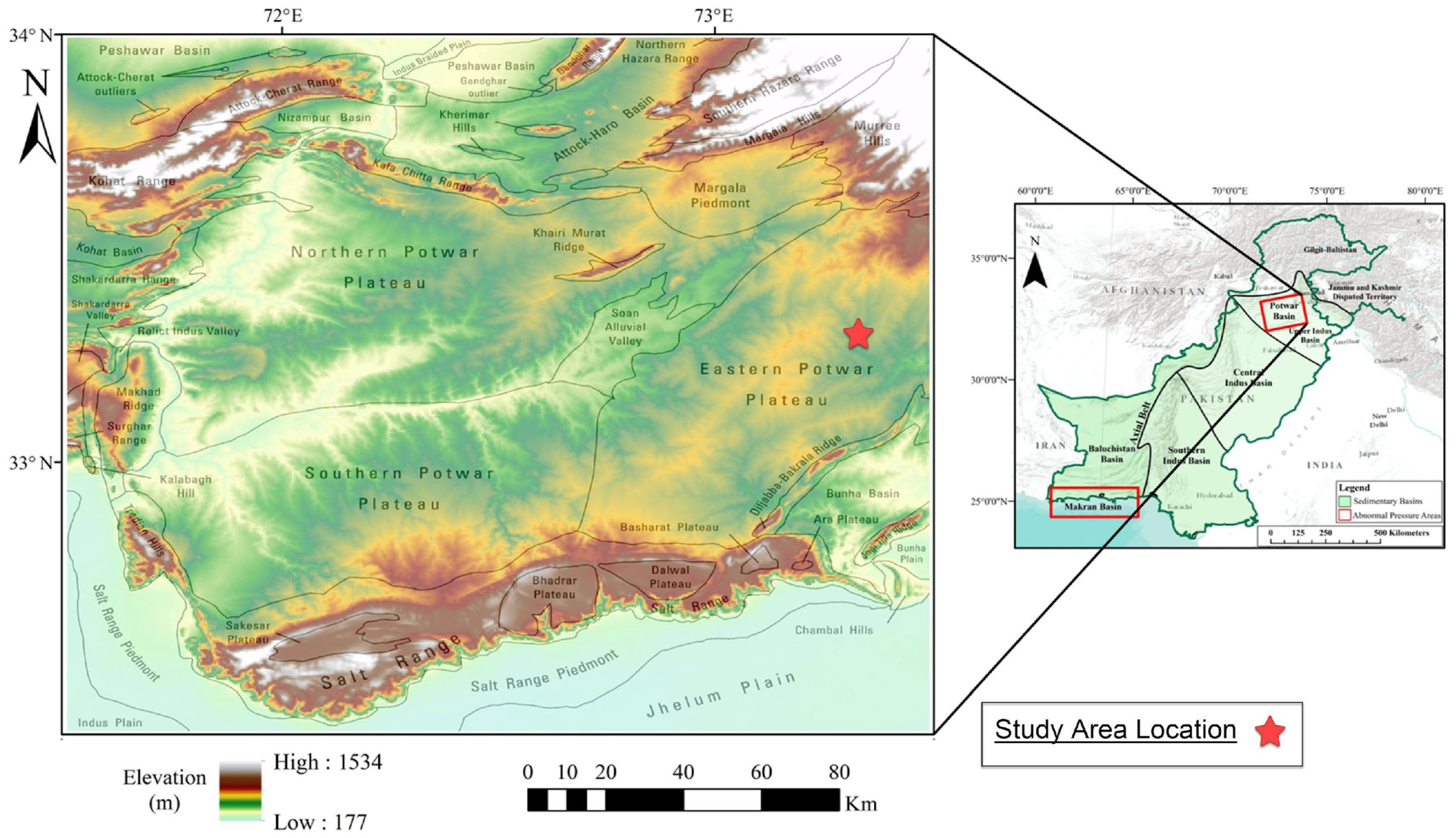
Well log data from the Missa Keswal oil field of Potwar Basin, Pakistan, has been used for pressure prediction (Figure 2). A total of four wells have been selected for the ML-based pressure prediction including Qazian-1X, Missa Keswal-01, Missa Keswal-02, and Missa Keswal-03. Missa Keswal-02 well is selected as the blind well for validation of results whereas the other three wells are utilized for data training. The research is focused on developing the generalizable pressure prediction model which can be used in unseen wells with limited data injection. The input data selected for data training comprises the well log data along with the computed petrophysical parameters of molasse deposits drilled in Qazian 1X, Missa Keswal-01, and Missa Keswal-03.
The well log data and the computed petrophysical parameters utilized during the data training for pressure prediction were initially prepared for the ML model input. The computed petrophysical properties for data training, as mentioned in Table 1, involve GR, DT, and RHOB curves. The PP curve computed with the help of Eaton’s [1] relation is calibrated with the measured pressure data of training wells. Specifically, the Qazian 1X well provided the most reliable results due to the availability of Drill Stem Test (DST) data as ground truthing for calibration and validation process. However, the PP curve for the rest of the wells has been calibrated with the available measured pressure or mud weight information. Details of the well log data, computed petrophysical properties, and utilized empirical relations are given in Table 1.
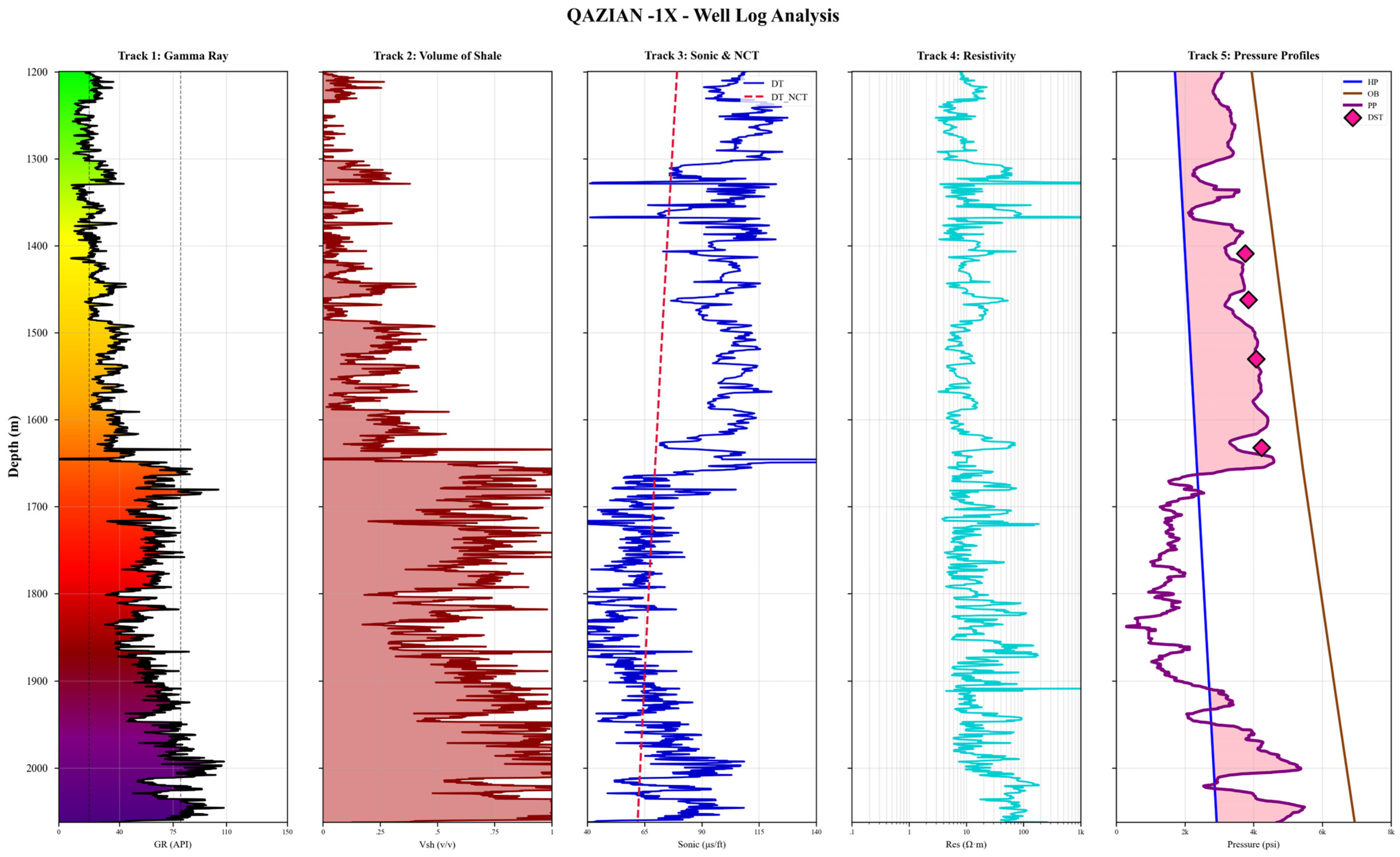
The input well log data and computed petrophysical properties for the Qazian 1X well are shown in Figure 3. A total of four tracks have been used to display the well log data of Neogene molasse deposits of the Potwar Basin. The plotted log data covers the depth interval from 1199 to 2063 m. The GR curve (track 1) and Vsh (track 2) indicate clean lithology at a shallower depth whereas the radioactivity is higher at a greater depth due to more percentage of clay minerals. High DT values in the upper part of the strata indicate more porosity, whereas the well shows a decreasing trend with an increase in clay percentage. Defining the NCT curve is the most critical part in pore pressure prediction. Sediments buried under the normal compaction exhibit a consistent and smooth decrease in porosity with fluid expulsion. Therefore, in slow sedimentation, porosity may decrease at a predictable rate with an increase in burial depth. This is marked by defining the normal compaction trendline using the DT curve. Track 1 in Figure 3, Figure 4 and Figure 5 uses a continuous color gradient to represent depth. The shallowest sections appear in green, and the depth increases as the colors transition through the spectrum, reaching purple for the deepest intervals.
The input well log data also includes the resistivity log curve which is displayed in track 4 of Figure 3. As the resistivity of the rocks is controlled by the fluid type, utilizing the deep resistivity curve in pressure prediction plays a significant role. Track 5 of Figure 3 represents the pressure profile of the stratigraphic interval computed through empirical relations. The HP represents the pressure of the overlying water column at a particular depth in the well whereas the OB is the weight of the overlying rock strata. The comparison of the PP curve with the HP indicates normal or abnormal pressure conditions. The four diamond points represent the DST data used for the calibration and validation of computed PP. This complete dataset is further utilized for predicting pore pressure through ML and DL models.
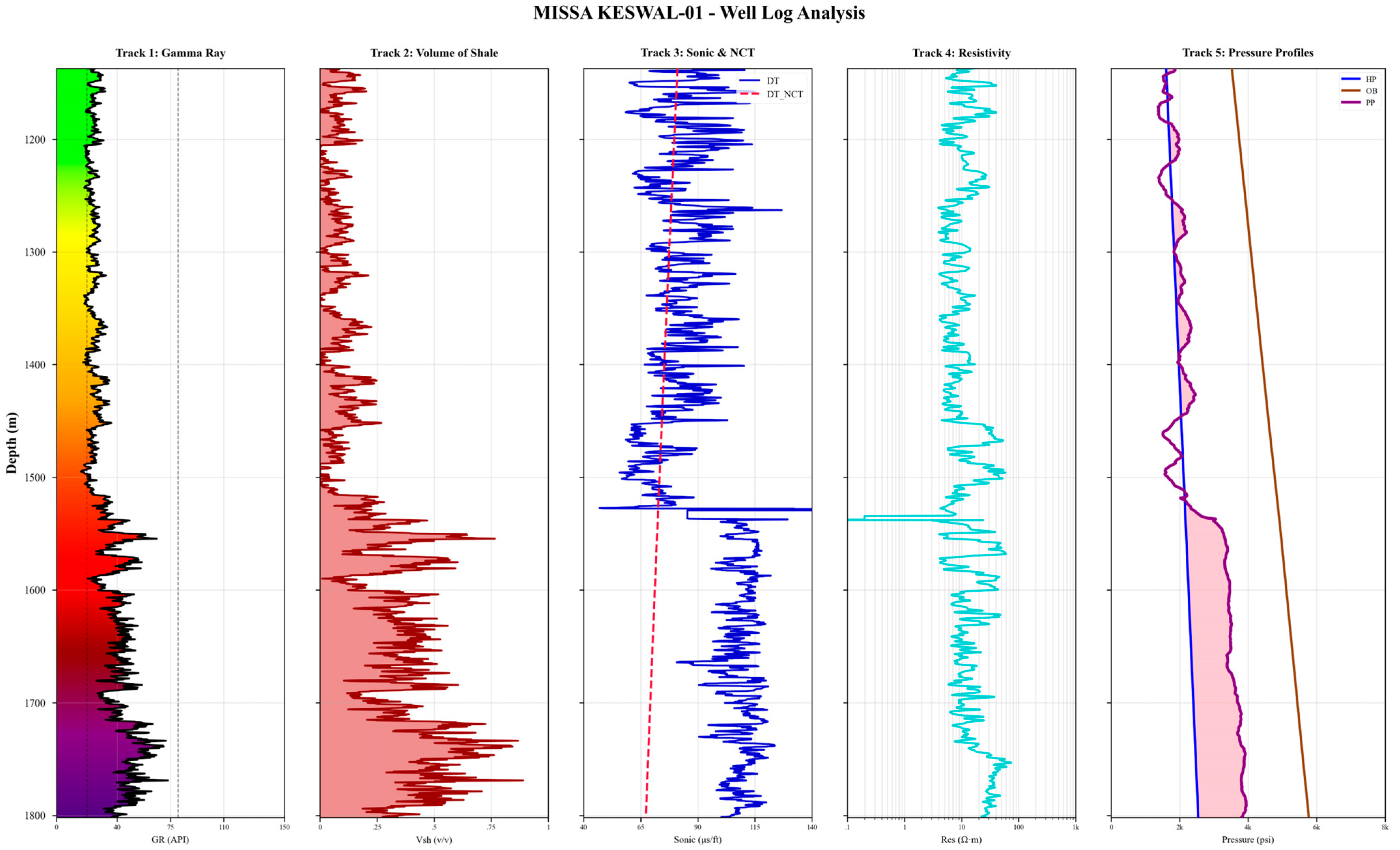
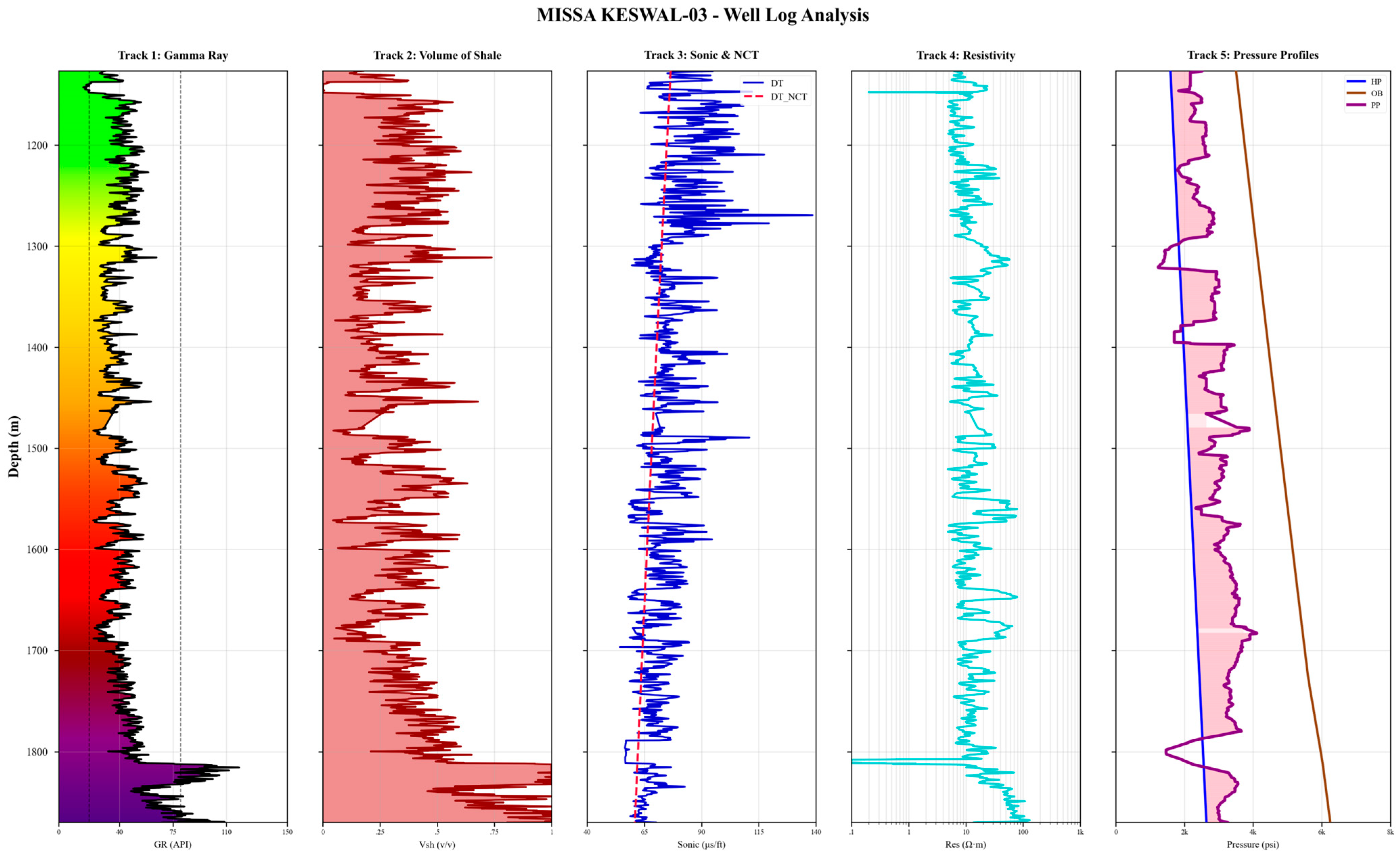
The well log data of the Missa Keswal-01 and Missa Keswal-03 wells are shown in Figure 4 and Figure 5. The lithological interval under investigation drilled in the Missa Keswal-01 well shows a smooth GR curve in the upper part (Figure 4). The lower part of the strata below 1500 m depth has a considerable increase in shale volume as shown by the Vsh curve resulting in deviation of DT curve from the NCT. This part also indicates overpressured conditions in the well. On the other hand, in the Missa Keswal-03 well (Figure 5), the formation represents a consistent GR trend with relatively high Vsh as compared to the Missa Keswal-01 well. The gradual decrease in the DT values with increasing depth depicts that the formation roughly follows the normal compaction profile; however, the persistent clay percentage developed some overpressuring due to limited fluid flow within the rock strata.

3.4. Performance Evaluation

For performance evaluation of the proposed model, the coefficient of determination R2, Mean Squared Error (MSE), Mean Absolute Error (MAE), and Relative Mean Squared Error (RMSE) are calculated [11,12,16,17].

3.4.1. Coefficient of Determination (R2)

The coefficient of determination (R2) measures the proportion of variance in the target variable (pore pressure) explained by the model predictions [12,17,18]. It quantifies the explained variance and overall predictive strength. It is calculated as follows:
R 2 = 1 i = 1 n y i ŷ i 2 i = 1 n y i ȳ 2
where yi represents the actual pore pressure values, ŷi represents the predicted values, and ȳ is the mean of actual values for n number of samples. R2 ranges from negative infinity to 1, where 1 indicates perfect prediction, 0 indicates performance equivalent to simply predicting the mean of the target variable, and negative values indicate performance worse than a mean predictor. This metric is particularly valuable for assessing model performance on blind wells, where negative R2 values reveal fundamental generalization failures.

3.4.2. Mean Absolute Error (MAE)

The Mean Absolute Error (MAE) provides an intuitive measure of average prediction error in the original units (psi) [4,12,17]:
MAE =   1 n   y i ŷ i
MAE is less sensitive to outliers compared to squared error metrics and provides a direct interpretation of typical prediction deviation. In the context of pore pressure prediction, MAE represents the average magnitude of pressure prediction errors, which is crucial for operational decision-making during drilling operations [14,19].

3.4.3. Root Mean Square Error (RMSE)

The Root Mean Square Error (RMSE) penalizes larger errors more heavily than MAE. It emphasizes large deviations and reflects prediction stability. It is calculated as follows:
RMSE =   1 n y i ŷ i 2
RMSE provides error measurement in the same units as the target variable (psi) while being more sensitive to large deviations [17,18]. This sensitivity is particularly important in pore pressure prediction, where large errors can have severe safety and economic consequences [25]. The RMSE serves as our primary metric for model comparison due to its widespread adoption in regression tasks and its mathematical properties that facilitate optimization.

3.4.4. Relative Root Mean Square Error (RelRMSE)

RelRMSE expresses RMSE as a percentage of actual values for a scale-free comparison. Thus, to enable comparison across different pressure ranges and wells with varying pressure regimes, the Relative RMSE is computed as a percentage [17]:
RelRMSE   ( % )   =   R M S E y m a x y m i n 100
where ymax and ymin represent the maximum and minimum pore pressure values in the test dataset. This normalization allows for meaningful comparison of model performance across different geological settings and pressure ranges. A RelRMSE below 10% is generally considered acceptable for operational pore pressure prediction applications.

4. Results

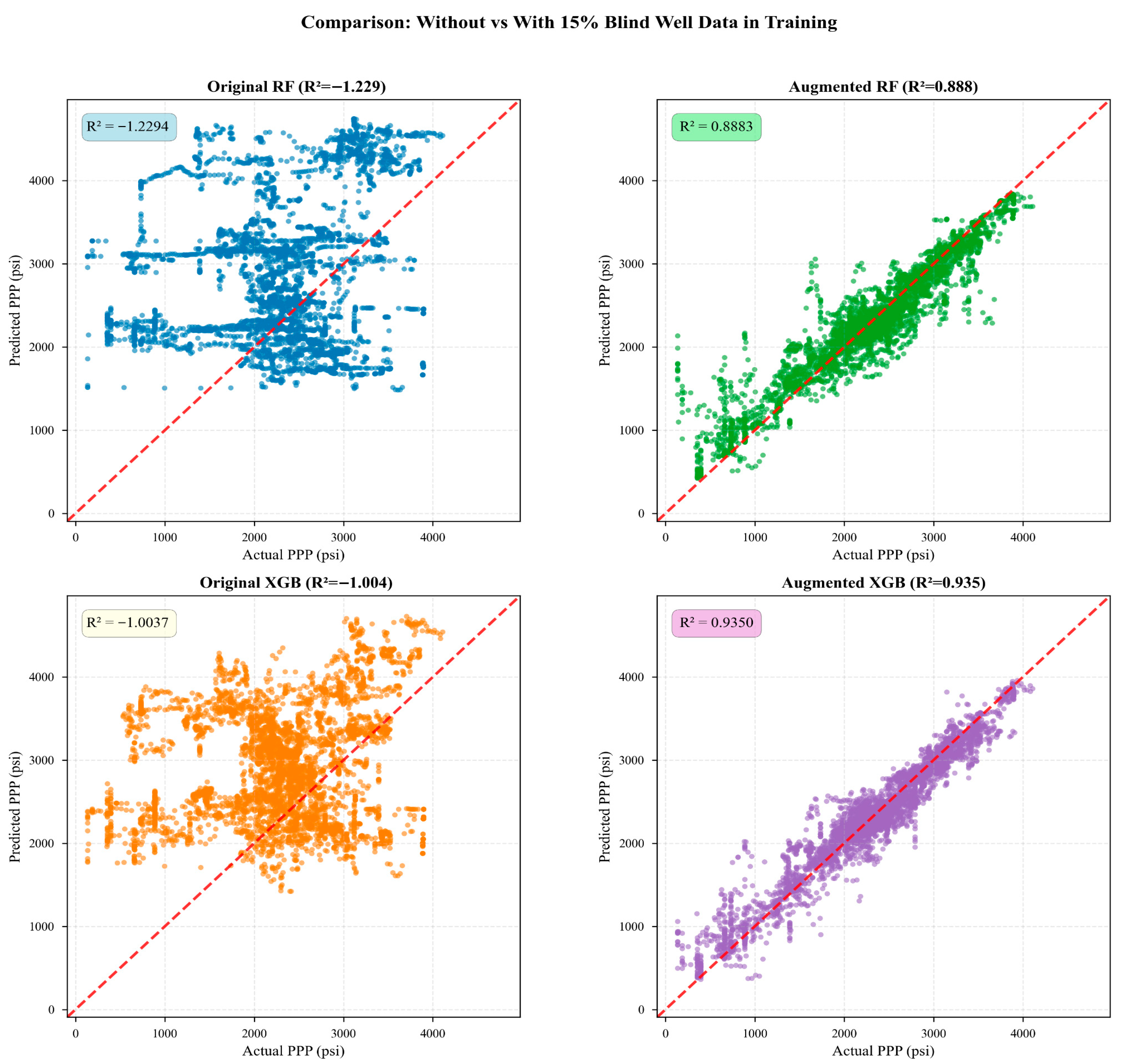
This section provides a comprehensive evaluation of five base ML models and their meta-ensemble combinations for blind well prediction. The experimental results demonstrate the critical importance of fine-tuning and the superior performance of ensemble methods, particularly stacking approaches. The initial blind well testing revealed significant challenges in achieving cross-well generalization, with all models exhibiting negative R2 values (Table 2). This indicates that the model’s predictions were worse than simply using the mean value of the target variable, suggesting substantial geological heterogeneity between the training and test wells. However, fine-tuning with 15% samples from the blind well produced remarkable improvements across all models.

4.1. Base Models

4.1.1. Convolutional Neural Networks

The CNN, despite its sophisticated convolutional architecture, achieved modest fine-tuned performance among all models (R2 = 0.7692). The 1D convolutions with kernel size 2 were designed to capture local feature patterns [5], but with only seven input features, the spatial structure that CNNs excel at exploiting was limited. The relatively high dropout rates (0.25–0.4) and strong L2 regularization, while preventing overfitting, may have constrained the model’s ability to fully adapt to the new well’s characteristics. However, CNN demonstrated the lowest performance among fine-tuned models, suggesting that the spatial feature extraction capabilities of CNNs may be less suited to this particular prediction task.

4.1.2. Recurrent Neural Networks

The RNN maintained consistent performance with R2 = 0.7712 after fine-tuning. While the improvement was substantial (ΔR2 = 1.5875), the model’s complex LSTM architecture required more careful adaptation. The higher training epochs (150 vs. 100 for other neural networks) and smaller batch size (16 vs. 32) reflected the increased computational demands and sensitivity of recurrent architectures.

4.1.3. Deep Feedforward Neural Networks

Among the neural networks, the DFNN showed the most dramatic improvement, jumping from the worst performer to achieving R2 = 0.7878. The carefully tuned dropout rates (0.1–0.2) specifically optimized for tabular data proved crucial in preventing overfitting during fine-tuning while allowing the network to adapt its learned representations. The progressive reduction in dropout from input to output layers helped preserve important feature information while still providing regularization.

4.1.4. Random Forest

RF secured the second-best performance post-fine-tuning (R2 = 0.8883, RMSE = 270.77 psi). The ensemble of 500 trees provided sufficient model capacity to capture the complexity of the new well while the bootstrap aggregation helped prevent overfitting to the limited fine-tuning samples. The controlled tree depth (max_depth = 15) struck an effective balance between expressiveness and generalization.

4.1.5. Extreme Gradient Boost

XGBoost emerged as the best-performing base model with an R2 of 0.9350 after fine-tuning, compared to −1.0037 initially. This improvement in R2 value is a testament to gradient boosting’s ability to rapidly adapt to new data distributions. The iterative nature of XGBoost, combined with its tree-based structure that naturally captures feature interactions, allowed it to quickly recalibrate to the blind well’s specific pressure–feature relationships.

4.2. Hybrid Meta-Ensemble

Three meta-ensemble approaches were evaluated to combine predictions from fine-tuned base models. Table 3 presents the performance metrics for each ensemble method.
The meta-modeling approaches of proposed HME demonstrated the power of combining diverse predictions. The stacking ensemble achieved outstanding performance (R2 = 0.9382, RMSE = 201.34 psi), surpassing even the best individual model. This 0.003 improvement in R2 over XGBoost alone may seem modest, but the reduction in RMSE and MAE represents meaningful improvements in prediction accuracy for critical drilling decisions.
The weighted average (R2 = 0.8711) outperformed the simple average (R2 = 0.8645), confirming that accounting for individual model strengths improves ensemble predictions. However, the stacking approach’s performance demonstrates that learning optimal nonlinear combinations of base model predictions captures complementary patterns that simple weighting schemes miss.
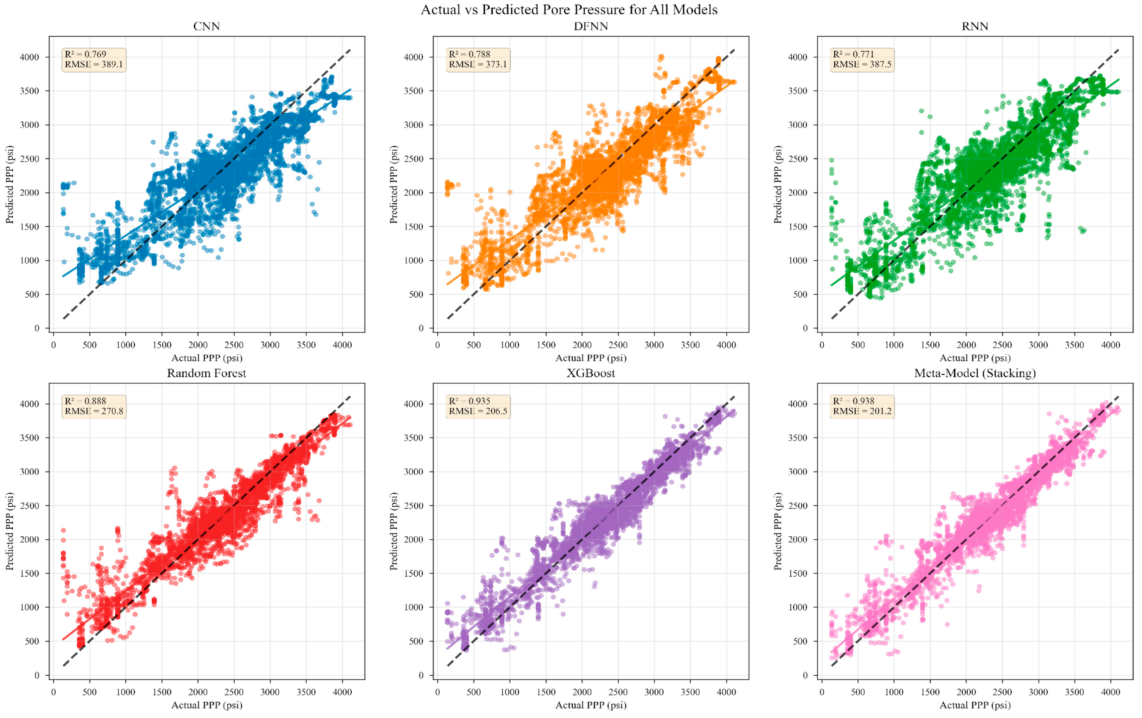
The scatter plot of Figure 6 clearly shows a performance ranking amongst the models, with neural networks (CNN, DFNN, RNN) having average prediction accuracy (R2 ~0.77) and high scatter especially at outlier pressure values, while tree-based ensemble models show better performance, culminating in XGBoost (R2 = 0.935) and the Meta-Model (R2 = 0.936) having near-perfect overlap along the diagonal line with extremely low RMSE (~200 psi); this verified the meta-ensemble approach’s ability to model complex nonlinear relationships between well logs and PP under different geological conditions.
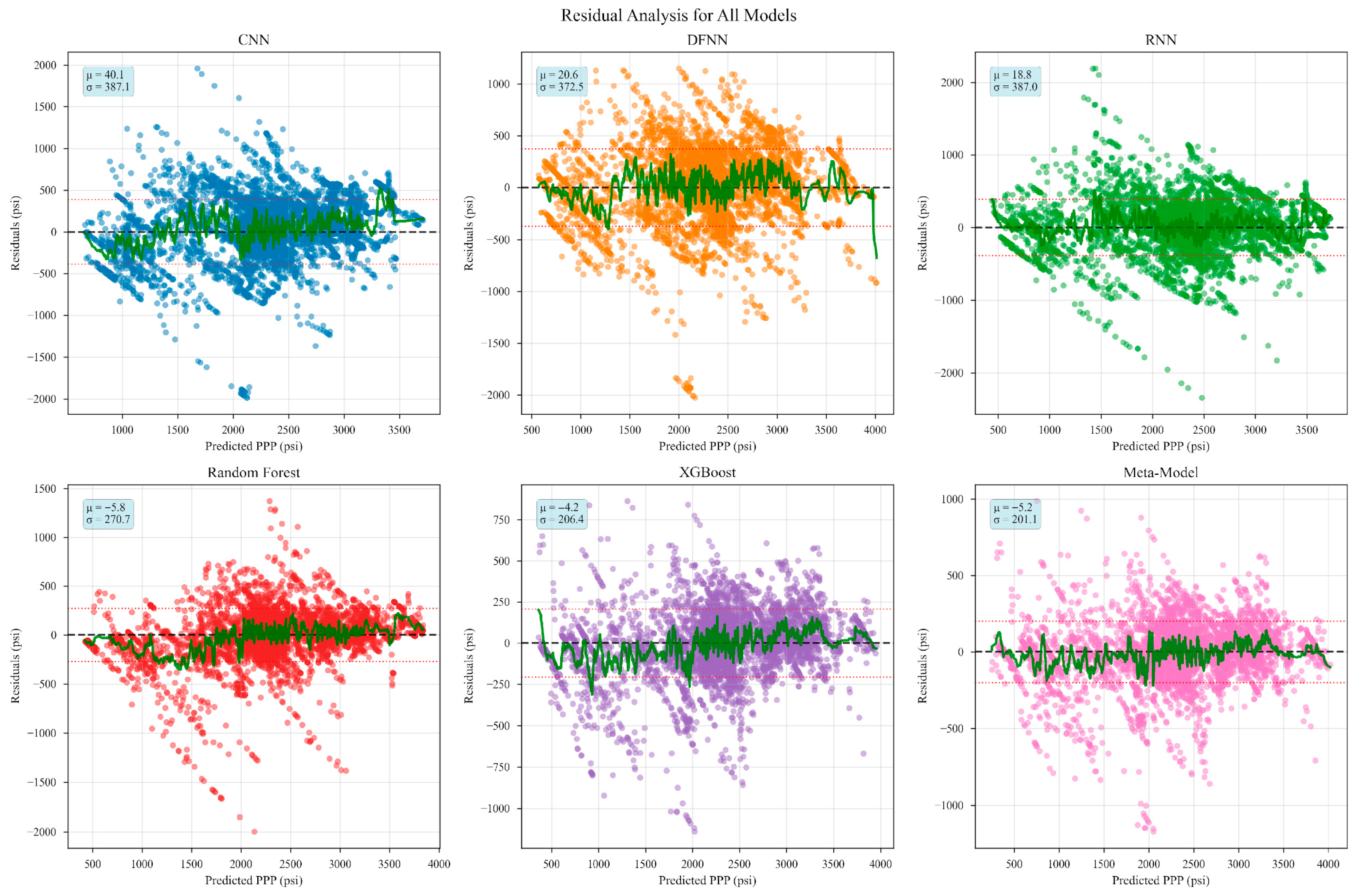
Figure 7’s residual plots reveal systematic patterns in model errors across the pressure range, with the neural network models (CNN, DFNN, RNN) displaying heteroscedasticity with growing variance at higher pressure, while ensemble techniques (Random Forest, XGBoost, Meta-Model) demonstrate more homoscedastic residuals around zero, reflecting better calibration with the Meta-Model having the least residual correlation (ρ = −5.2) and suggesting minimal systematic bias across the prediction range.

4.3. Comparative Analysis and Model Selection

The experimental results of the base models reveal several key findings in respect to pressure prediction which are discussed below:
(a)
Critical Importance of Fine-tuning: All models exhibited negative R2 values before fine-tuning, indicating unreliable predictions. Fine-tuning transformed these models into effective predictors, with R2 improvements ranging from 1.72 to 2.19 units.
(b)
Model Hierarchy: Among base models, performance ranking after fine-tuning was XGBoost > RF > RNN > DFNN > CNN. Tree-based ensemble methods (XGBoost and RF) demonstrated superior performance, likely due to their ability to capture complex nonlinear relationships without requiring extensive feature engineering.
(c)
Ensemble Superiority: The stacking meta-ensemble achieved the best overall performance (R2 = 0.9382), demonstrating that sophisticated model combination strategies can exceed individual model capabilities. The 39.9% improvement over simple averaging highlights the value of learned combination weights.
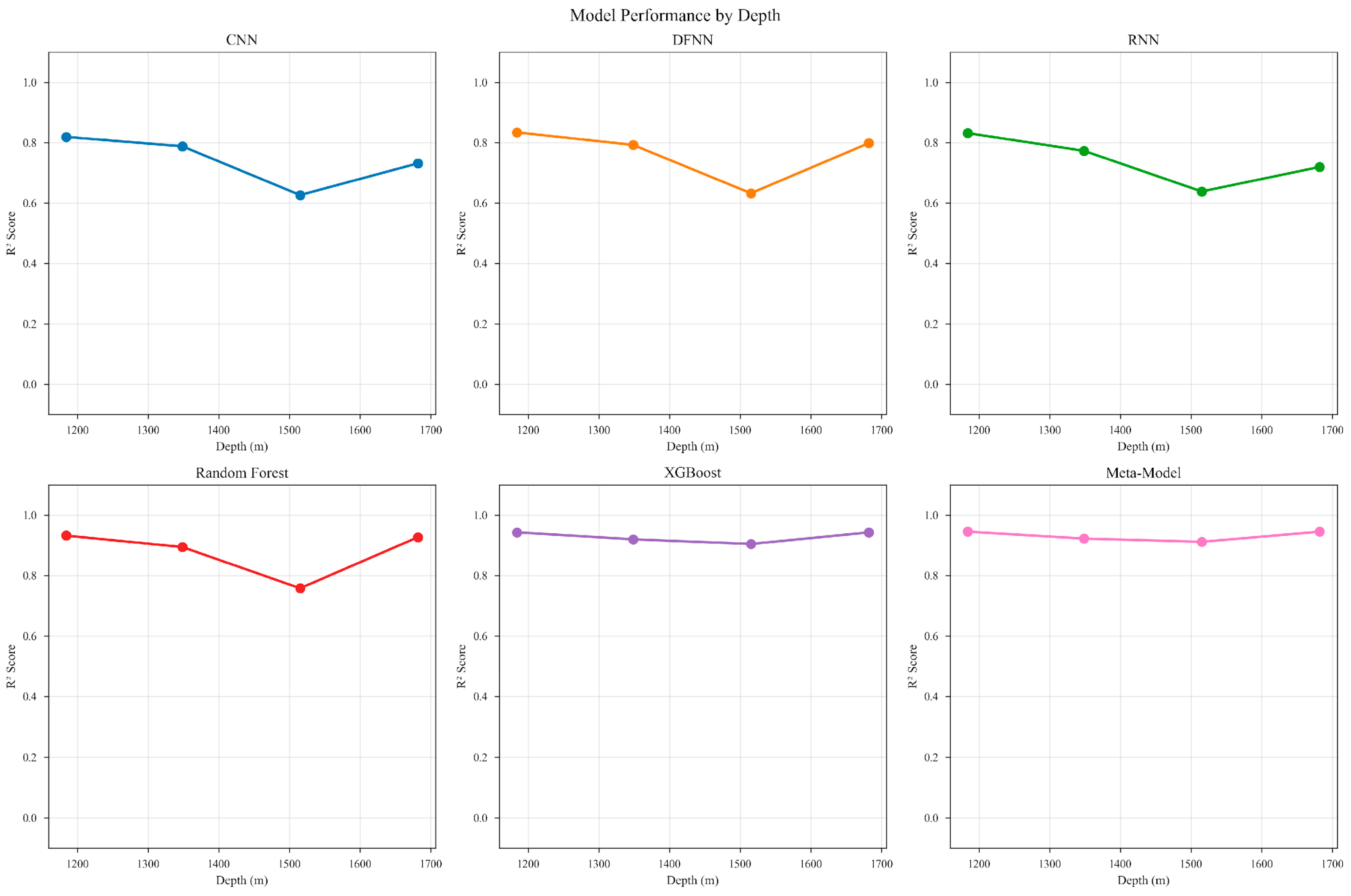
The stratified performance graph in Figure 8 shows that all models achieve the highest R2 values within the range of shallow depth (1150–1350 m), where common compaction trends dominate and perform weakly at shallow depths with unconstrained sediments, and at deeper depths, where complex diagenetic effects and pressure mechanisms have a greater influence, and XGBoost performed most consistently over all depth ranges.
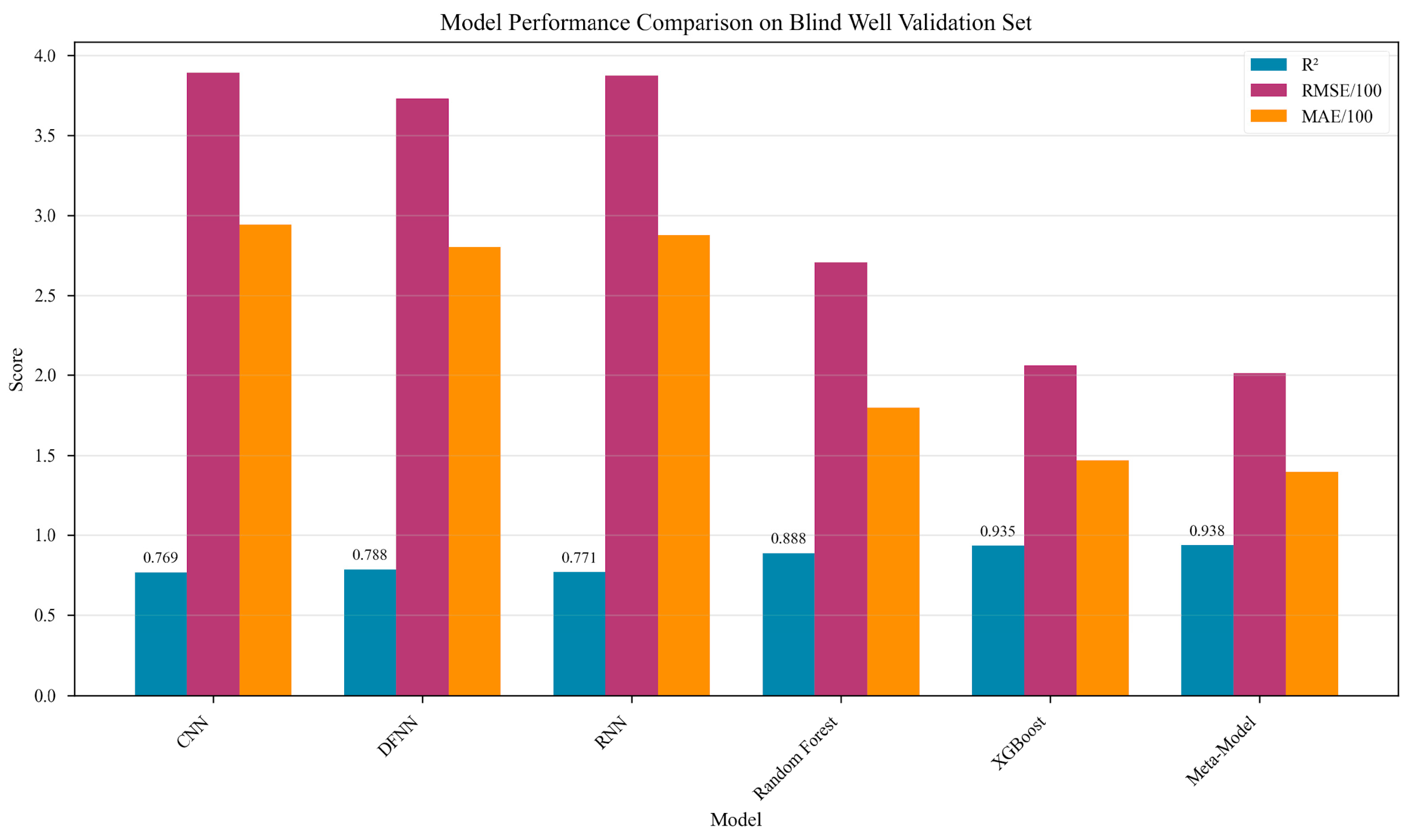
The model performance comparison on the blind well validation set shown in Figure 9 compares six models on a blind well validation set using (R2), RMSE/100, and MAE/100 metrics. Ensemble models (RF, XGBoost, and Meta-Model) outperform DL models (CNN, DFNN, and RNN), achieving higher (R2) scores and lower errors. The Meta-Model shows the best performance overall, indicating superior predictive accuracy and generalization.
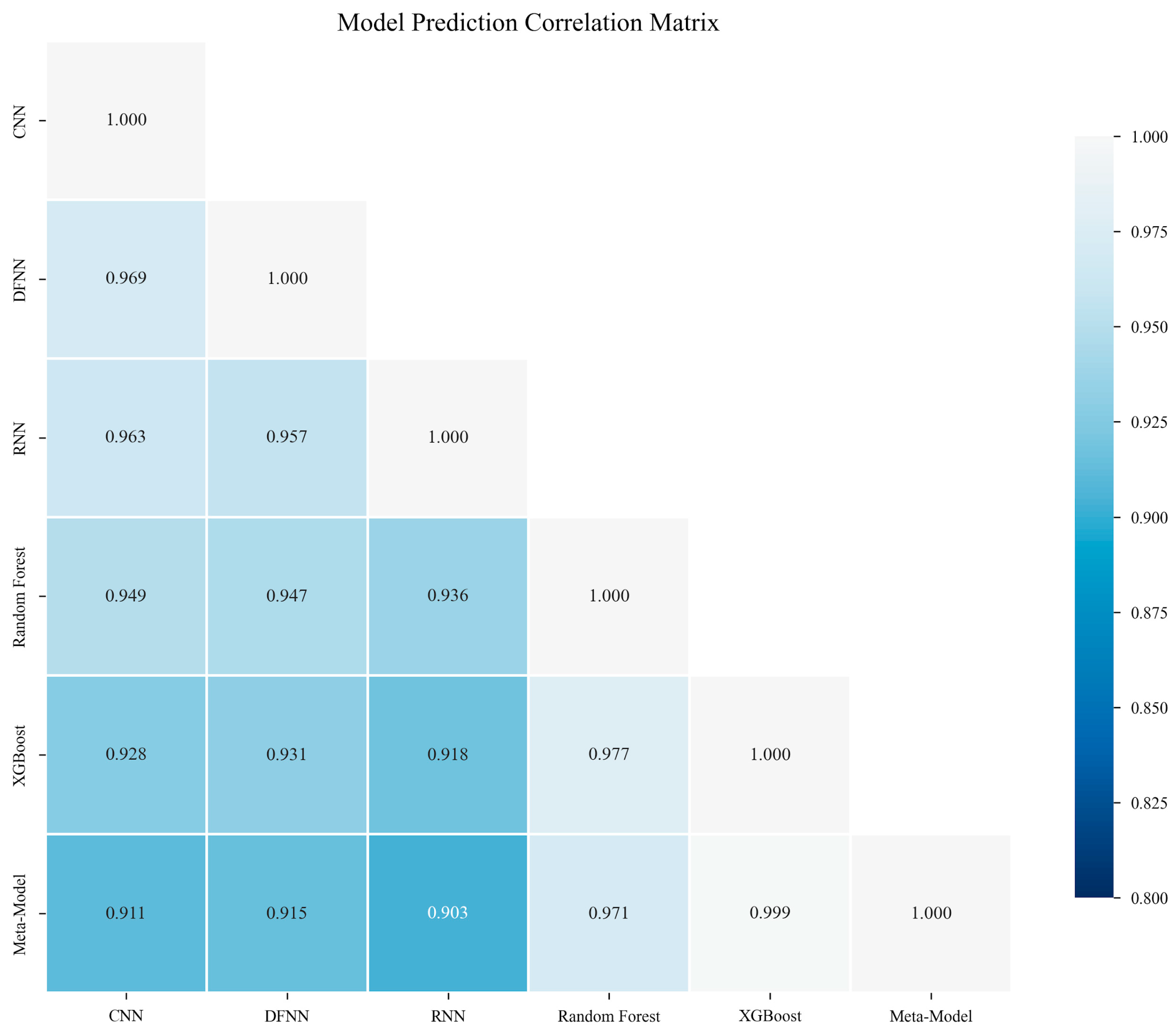
Figure 10’s correlation matrix illustrates high inter-model consistency (correlations > 0.85) across neural network models and separately across tree-based models but moderate correlation (~0.7) across model families, suggesting that different architectures explain complementary patterns in data and warrant the ensemble approach, leveraging diverse views of models for improved predictions.
The dramatic increase in Figure 11 from R2 = −1.22 to R2 = 0.888 using the RF model and R2 = −1.004 to R2 = 0.935 for the XGBoost model with the addition of just 15% blind well data indicates that small amounts of target domain data enable substantial domain adaptation, compressing scattered predictions into tightly aligned estimates on the diagonal, suggesting that selective data injection can bridge geological differences between training and test wells.
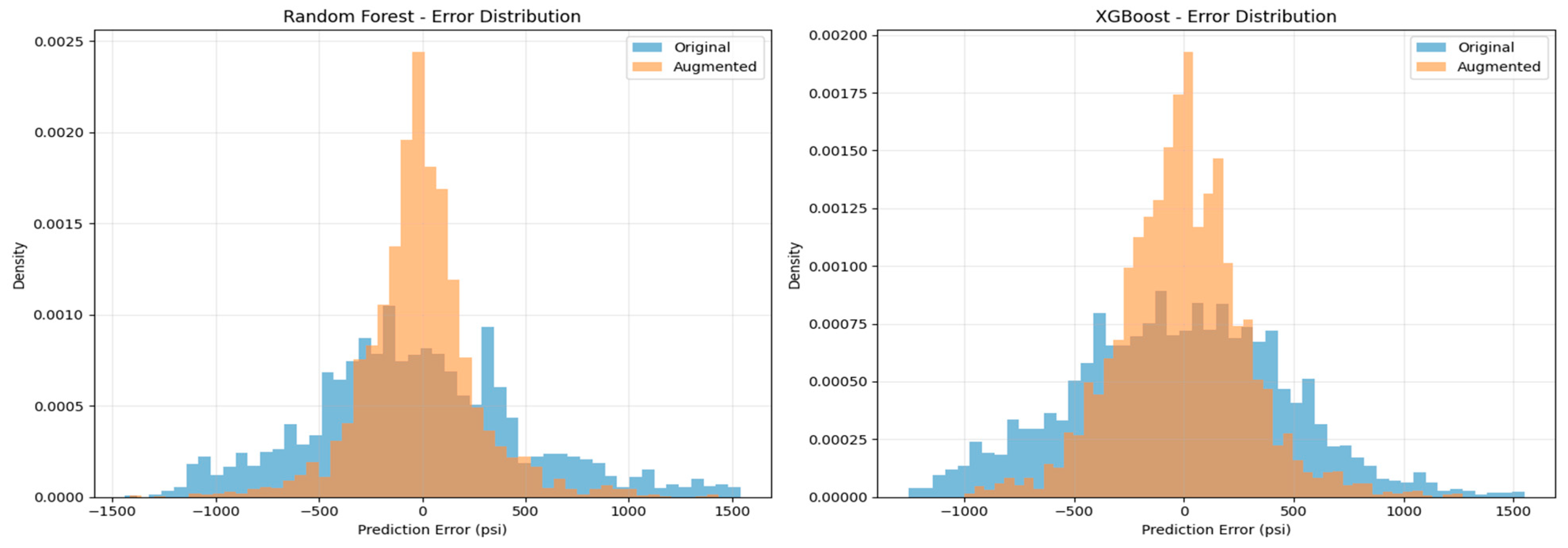
The error distribution comparison in Figure 12 shows the better models transforming broad, heavy-tailed error distributions into thin, nearly Gaussian distributions centered on zero, where standard deviation is reduced by roughly 60%, indicating that domain adaptation not only improves mean accuracy but also improves prediction resilience and reduces catastrophic failure.

4.4. Pressure Prediction in Blind Well

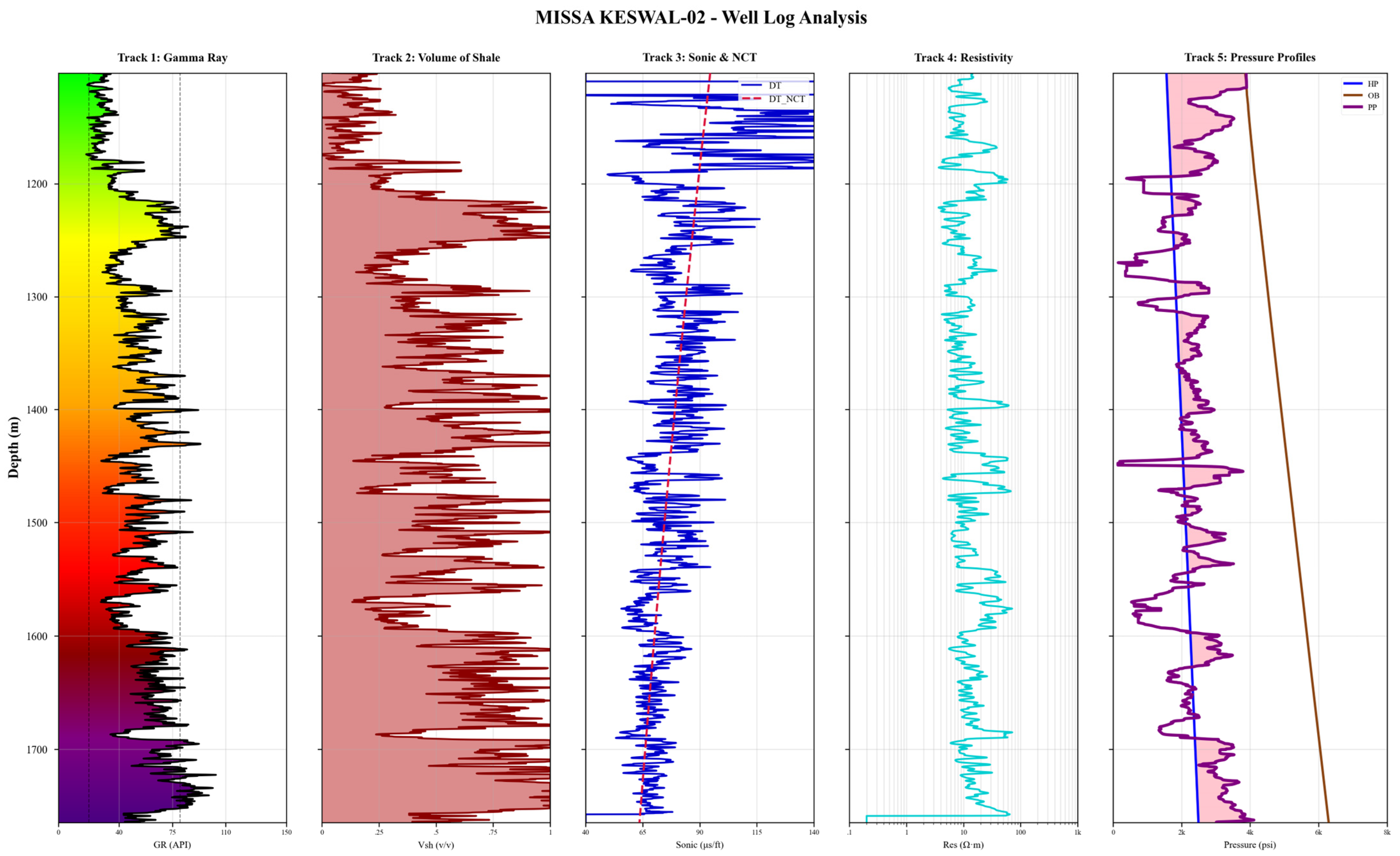
The composite logplot of Missa Keswal-02, selected as a blind well, is shown in Figure 13 displaying the input parameters and pressure profiles. The logplot displays five key petrophysical tracks versus depth for the Missa Keswal-02 well: GR and Vsh to demarcate sand and shale intervals, DT and NCT showing the impact of compaction with the increase in depth, sonic porosity (SPHI) to understand the porosity variations, and lastly, the pressure profiles highlighting HP, OB, PP, and predicted pressure curves. The colored shading demarcates the intervals of overpressure and underpressure strata that are critical for identifying abnormal pressure intervals in evaluating drilling safety.
Neogene molasse sediments under investigation show a relatively higher shale percentage in Missa Keswal-02 well with thin, clean sand intervals. The DT profile displayed in track 3 of Figure 13 shows a gradual decrease in values indicating increased compaction with burial depth. This compaction rate is also complemented by the porosity reduction. The normal compaction trendline in most of the strata indicates that the sediments have undergone normal compaction except for a few intervals. These overpressured intervals are highlighted by the color fill in the pressure profile track where computed pore pressure is greater than hydrostatic pressure. The correlation of these overpressured intervals with the porosity curve indicates that the fluid is trapped within the high porous sand packages leading to abnormal pressure conditions.
The overpressured intervals in the Missa Keswal-02 well exhibits higher than the anticipated porosity that would normally occur under normal compaction. As a result, higher porosity is preserved within the rock in response to low effective stress, hydraulic isolation, and low permeability. This indicates undercompaction of the sediments, and the fluid was unable to expel out of the pores during burial. The retained fluid counters overburden pressure and restricts mechanical compaction while preserving porosity at greater depth. The presence of overpressured zones within these preserved porosities is caused by the high rate of sedimentation resulting in compaction disequilibrium.
The pressure profiles also show the correlation of the calibrated well-based pore pressure (purple) with the ML-predicted pressure (pink) curve. The 15% data injection from the blind well during data training provided a very good correlation between the predicted pressure and pore pressure. The Meta-Model achieves more than 93% correlation coefficient, having an R2 of 0.9382 with an RMSE value of 201.34 psi. The results, computed through the stacking approach of the model, efficiently address rock heterogeneity by learning optimal nonlinear combinations of base models.

4.5. Leave-One-Well-Out Cross-Validation (LOOCV)

The four-fold cross-validation was performed as each of the four wells; QAZIAN-1X, MISSA_KESWAL-01, MISSA_KESWAL-02, and MISSA_KESWAL-03 were tested in turn as the blind test well, with the remaining three used for training, to perform a total of four independent evaluation folds. This form of Leave-One-Well-Out Cross-Validation (LOWO-CV) is stronger than the traditional random split validation in assessing the generalization of the models because it ensures that the test well is from a completely unseen geological setting with potentially different depositional environments, compaction histories, and pressure generation mechanisms. By systematically using all available wells as test cases in sequence, LOWO-CV quantifies not only the average performance but also the model prediction variance over heterogeneous geological conditions, offering key insights into model stability. This methodology will be particularly relevant for applications of pore pressure predictions, which require models to generalize across a wide variety of structural compartments within a basin since every well may present a unique lithological sequence, diagenetic alteration, and pressure regime to challenge the representation learned by the model. In fact, comprehensive evaluation across all permutations avoids performance metrics biased by fortuitous similarity between specific training–test well pairs, therefore offering realistic operational deployment scenarios. The results obtained for LOWO-CV are shown in Table 4.
The LOOCV analysis on four representative wells (QAZIAN-1X and MISSA_KESWAL 01–03) demonstrates strong generalization capabilities. As shown in Table 4, the Meta-Model achieved the highest mean R2 of 0.959 with minimal variance across folds, validating its robustness to well-specific geological variations. Tree-based models significantly outperformed neural networks, with XGBoost and Random Forest maintaining R2 above 0.94, while neural architectures showed higher variance and lower overall performance with R2 of 0.83.

5. Discussion

Maintaining a sustainable global energy system has become one of the challenging tasks consistent with increases in energy demands [26]. To meet energy demands, effective drilling strategies are necessary, having comprehensive information of formation pressure [27]. The experimental results of the proposed HME framework demonstrate its effectiveness with precise and enhanced pore pressure prediction in complex geological environments. The method integrates diverse baseline methods and was able to capture hidden relationships in well log data. The meta-ensemble model also showed great predictive accuracy, outperforming all individual base models. The ability of the meta-ensemble model over individual models, particularly XGBoost, highlights HME’s ability to exploit cross-model dependencies and learn optimal nonlinear combinations. The increase in R2 may appear small but the reductions in RMSE and MAE are significantly meaningful for drilling applications where pressure deviations of even a few hundred psi can greatly impact safety and cost.
Among the baseline models, tree-based methods (RF and XGBoost) consistently outperformed deep neural network architectures. This aligns with the established understanding from the existing literature that decision tree-based methods handle tabular and heterogeneous data more effectively [28,29]. On the other hand, CNN’s performance (R2 = 0.7581) shows its reliance on strong spatial locality, while RNN’s moderate results (R2 = 0.7826) show that depth-wise sequential patterns were insufficient to capture broader geological variability. The DFNN, however, achieved competitive performance (R2 = 0.7901), demonstrating that simpler feedforward models can learn useful nonlinear mappings when regularized adequately. Overall, the performance hierarchy observed (XGBoost > RF > RNN > DFNN > CNN) shows the dominance of boosted tree ensembles for cross-well learning; still, the complementary nature of neural and statistical models remains essential for ensemble synergy.
A significant performance in results is achieved after fine-tuning with 15% of blind well data injection. This shows the role of domain adaptation in geological machine learning. All models initially produced negative R2 values when directly tested on the blind well. This shows severe domain shift due to lithological and depositional variations across wells. Injecting a small fraction of blind well samples has effectively bridged this gap. This adaptive retraining enabled the model to recalibrate for a new geological regime without overfitting. This also confirms the feasibility of limited target domain sampling as a practical solution for real-word deployment in geological settings. Furthermore, the narrowing of error distributions as shown in Figure 12 shows that fine tuning not only improves mean accuracy but also reduces variance, enhancing the model’s reliability for drilling safety.
The decision tree models can perform better than the neural networks in predicting pore pressure from well data [30,31]. The moderate correlation between neural networks and the tree-based models shows that each architecture captures distinct geological settings. The effectiveness of HME stems from its ability to capture inter-model relationships (Figure 10). The meta learner trained on stacked predictions effectively integrates these complimentary signals and delivers stable estimates across varying lithological contexts.
From a geophysical perspective, the results illustrate that pore pressure prediction benefits from an integrative approach combining geological indicators. The model’s consistent performance across varying depths (Figure 13) shows that ensemble framework captures both local pressure anomalies and broader formation competition trends. The enhanced prediction accuracy in shallow (1150–1350 m) and deeper depth ranges (1550–1700 m) corresponds to zones dominated by normal compaction, whereas performance degradation at medium depth (1350–1550 m) aligns with known complexities due to unconsolidated sediments and overpressure mechanisms.
Operationally, the HME framework offers a scalable solution for real time drilling support. By leveraging limited blind well samples for fine-tuning, the approach can be readily adapted to new basins having at least one exploratory well, providing a valuable tool for pore pressure estimation and risk mitigation. This might not only contribute to facilitating safe and secure drilling but it also effectively reduces non-productive drilling time. The precision and accuracy of predicted pressure profiles can significantly contribute towards borehole stability and integrity in complex geological settings.
Future iterations could incorporate real-time drilling parameters (ROP, WOB, torque) and physics-based transformations like acoustic impedance to enrich the feature space. Synthetic feature generation using variational autoencoders could potentially improve accuracy by 5–10% based on preliminary experiments. Operational deployment requires real-time data infrastructure processing of 50+ samples/second and adaptive retraining triggered by >20% distribution shifts. The HME framework can help in the integration of existing drilling software and failsafe mechanisms defaulting to physics-based models when ensemble disagreement exceeds thresholds and ensures operational safety. Despite the promising results of HME, there are limitations that are under consideration. The model’s reliance on the limited features constrains its ability to fully capture the multifactorial nature of pore pressure. Incorporating further domain engineered attributes like normalized rate of penetration, velocity deviation ratio, compaction coefficient, porosity reduction rate, and, most importantly, measured pressure data can further enhance its prediction power. Apart from that, while the controlled exposure of blind well data improved generalization, real-world deployment would require systematic domain adaptation strategies.

6. Model Limitations

Despite the encouraging performance of the Hybrid Meta-Ensemble framework, several limitations provide avenues for further research. The framework’s primary constraint is its reliance on target well data for effective domain adaptation, requiring approximately 15% of blind well samples (785 samples in our setup) to achieve adequate performance. Additionally, each constituent model exhibits specific architectural limitations: CNNs struggle with long-range depth dependencies (R2 dropping to 0.67 in transition zones); RNNs suffer from vanishing gradients in deep sequences, limiting their ability at geological boundaries; DFNNs lack spatial awareness, resulting in 25% accuracy drops at formation interfaces; while tree-based models (RF and XGBoost) show limited extrapolation capability outside training ranges and produce stepped predictions in continuous pressure zones. The meta-ensemble partially mitigates these through complementary strengths, but residual errors persist in extremely heterogeneous formations.
The ensemble imposes a significant computational cost: the proposed ensemble solution needs six times more resources compared to single-model solutions, increasing the prediction times from 0.05 up to 0.3 s, with the memory requirements increasing from 400 MB up to 2.5 GB. Although tolerable in a research setting, these might be challenging for real-time deployment on edge computing devices used during drilling.

7. Conclusions

This study developed a Hybrid Meta-Ensemble framework integrating diverse ML and DL models, including CNN, RNN, DFNN, RF, and XGBoost, for pore pressure prediction across multiple wells of the Potwar Basin, one of the major gas- and oil-producing basins of Pakistan. The initial blind well evaluation showed limited generalization due to strong geological heterogeneity. However, fine-tuning with a small subset (15%) of blind well data significantly improved model performance, with individual learners achieving R2 values up to 0.93 and relative RMSE as low as 5%.
Correlation analysis of model predictions revealed complementary learning patterns that justify the ensemble approach. Neural networks (CNN-RNN correlation: 0.72) captured similar spatial–temporal features, while tree-based models (RF-XGBoost: 0.89) showed high agreement in their predictions. Importantly, neural networks exhibited weak correlation with tree-based methods (0.45–0.52), confirming diverse feature extraction strategies. The meta-model predictions demonstrated balanced correlation (0.65–0.75) with all base models, effectively synthesizing their complementary strengths. Leave-One-Well-Out Cross-Validation on four representative wells further validated the framework’s robustness, with the meta-ensemble achieving a mean R2 of 0.959 (±0.031) compared to individual models ranging from 0.825 to 0.957, demonstrating consistent performance across different geological contexts.
The stacking-based proposed HME achieved the best overall performance with an R2 of 0.9328, MAE of 140.05 psi, RMSE of 201.34 psi, and a relative RMSE of 5.07%. This establishes the advantage of hierarchical ensemble learning, where the meta learner effectively leverages complementary strengths of the base models to capture complex dependencies in the well log data. The framework’s ability to maintain high performance despite a 17.4% pressure regime shift between training and test sets demonstrates its practical applicability for field deployment.
Overall, the proposed HME achieves high predictive accuracy and demonstrates strong cross-well generalization to unseen geological data. These outcomes show that HME is an efficient data-driven tool for real-world pore pressure prediction, supporting safer and more efficient drilling operations. In the future, we plan to work towards a framework with explainable AI methods to quantify uncertainty and to improve interpretability of predictions in subsurface pressure estimation.

Author Contributions

Conceptualization, T.A. and M.R.A.; coding and implementation R.B.V.; validation, R.B.V. and M.R.A.; formal analysis, M.R.A.; investigation, R.B.V.; resources, M.R.A.; data curation, M.R.A.; writing—original draft preparation, M.R.A.; writing—review and editing, M.R.A., T.A., and R.B.V.; visualization, M.R.A. and R.B.V.; supervision, T.A.; funding acquisition, T.A. All authors have read and agreed to the published version of the manuscript.

Funding

This research is supported by Khoury College of Computer Science, Northeastern University under the Research Runway Program.

Data Availability Statement

The data used in the study is proprietary and can only be shared on request in a case-to-case basis.

Acknowledgments

During the preparation of this manuscript/study, the authors used Grammarly for the purposes of removing linguistic errors. The authors have reviewed and edited the output and take full responsibility for the content of this publication.

Conflicts of Interest

The authors declare that there is no conflict of interest.

Abbreviations

The following abbreviations are used in this manuscript:
MLMachine Learning
PPPPore Pressure Prediction
HMEHybrid Meta-Ensemble
CNNConvolutional Neural Network
RNNRecurrent Neural Network
DFNNDeep Feedforward Neural Network
RFRandom Forest
XGBoostExtreme Gradient Boost

References

  1. Eaton, B.A. The equation for geopressure prediction from well logs. In Proceedings of the SPE Annual Technical Conference and Exhibition, Dallas, TX, USA, 28 September–1 October 1975; p. SPE-5544-MS. [Google Scholar]
  2. Bowers, G.L. Pore pressure estimation from velocity data: Accounting for overpressure mechanisms besides undercompaction. SPE Drill. Complet. 1995, 10, 89–95. [Google Scholar] [CrossRef]
  3. Amjad, M.R.; Zafar, M.; Malik, M.B.; Naseer, Z. Precise geopressure predictions in active foreland basins: An application of deep feedforward neural networks. J. Asian Earth Sci. 2003, 245, 105560. [Google Scholar] [CrossRef]
  4. Li, H.; Tan, Q.; Deng, J.; Dong, B.; Li, B.; Guo, J.; Zhang, S.; Bai, W. A Comprehensive Prediction Method for Pore Pressure in Abnormally High-Pressure Blocks Based on Machine Learning. Processes 2023, 11, 2603. [Google Scholar] [CrossRef]
  5. Lawal, A.; Yang, Y.; He, H.; Baisa, N.L. Machine learning in oil and gas exploration: A review. IEEE Access 2024, 12, 19035–19058. [Google Scholar] [CrossRef]
  6. Yu, H.; Chen, G.; Gu, H. A machine learning methodology for multivariate pore-pressure prediction. Comput. Geosci. 2020, 143, 104548. [Google Scholar] [CrossRef]
  7. Amjad, M.R.; Shakir, U.; Hussain, M.; Rasul, A.; Mehmood, S.; Ehsan, M. Sembar formation as an unconventional prospect: New insights in evaluating shale gas potential combined with deep learning. Nat. Resour. Res. 2023, 32, 2655–2683. [Google Scholar] [CrossRef]
  8. Naseer, Z.; Ehsan, M.; Ali, M.; Amjad, M.R.; Latif, M.A.U.; Abdelrahman, K. Lithofacies and sandstone reservoir characterization for geothermal assessment through artificial intelligence. Results Eng. 2025, 26, 105173. [Google Scholar] [CrossRef]
  9. Elmgerbi, A.; Thonhauser, G. Assessing the Potential of Advanced Sensor Technologies and IoT in Predicting Downhole Drilling Issues. In Proceedings of the SPE Gas & Oil Technology Showcase and Conference, GOTECH, Dubai City, UAE, 21–23 April 2025. [Google Scholar] [CrossRef]
  10. Han, J.; Kamber, M.; Mining, D. Concepts and techniques. Morgan Kaufmann 2006, 340, 94104–103205. [Google Scholar]
  11. Zhang, J. Pore pressure prediction from well logs: Methods, modifications, and new approaches. Earth-Sci. Rev. 2011, 108, 50–63. [Google Scholar] [CrossRef]
  12. Krishna, S.; Irfan, S.A.; Keshavarz, S.; Thonhauser, G.; Ilyas, S.U. Smart predictions of petrophysical formation pore pressure via robust data-driven intelligent models, Multiscale Multidiscip. Model. Exp. Des. 2024, 7, 5611–5630. [Google Scholar] [CrossRef]
  13. Ahmed, A. New Model for Pore Pressure Prediction While Drilling Using Artificial Neural Networks. Arab. J. Sci. Eng. 2018, 44, 6079–6088. Available online: https://link.springer.com/article/10.1007/s13369-018-3574-7 (accessed on 11 September 2025).
  14. Abdelaal, A.; Elkatatny, S.; Abdulraheem, A. Data-Driven Modeling Approach for Pore Pressure Gradient Prediction while Drilling from Drilling Parameters. ACS Omega 2021, 6, 13807–13816. [Google Scholar] [CrossRef]
  15. Matinkia, M.; Amraeiniya, A.; Behboud, M.M.; Mehrad, M.; Bajolvand, M.; Gandomgoun, M.H.; Gandomgoun, M. A novel approach to pore pressure modeling based on conventional well logs using convolutional neural network. J. Pet. Sci. Eng. 2022, 211, 110156. [Google Scholar] [CrossRef]
  16. Huang, H.; Li, J.; Yang, H.; Wang, B.; Gao, R.; Luo, M.; Li, W.; Zhang, G.; Liu, L. Research on prediction methods of formation pore pressure based on machine learning. Energy Sci. Eng. 2022, 10, 1886–1901. [Google Scholar] [CrossRef]
  17. Radwan, A.E.; Wood, D.A.; Radwan, A.A. Machine learning and data-driven prediction of pore pressure from geophysical logs: A case study for the Mangahewa gas field, New Zealand. J. Rock Mech. Geotech. Eng. 2022, 14, 1799–1809. [Google Scholar] [CrossRef]
  18. Farsi, M.; Mohamadian, N.; Ghorbani, H.; Wood, D.A.; Davoodi, S.; Moghadasi, J.; Alvar, M.A. Predicting formation pore-pressure from well-log data with hybrid machine-learning optimization algorithms. Nat. Resour. Res. 2021, 30, 3455–3481. [Google Scholar] [CrossRef]
  19. Abdelaal, A.; Elkatatny, S.; Abdulraheem, A. Real-time prediction of formation pressure gradient while drilling. Nature 2022, 12, 11318. [Google Scholar] [CrossRef]
  20. Shi, L.; Tang, Z.; Zhang, N.; Zhang, X.; Yang, Z. A Survey on Employing Large Language Models for Text-to-SQL Tasks. ACM Comput. Surv. 2025, 58, 3737873. [Google Scholar] [CrossRef]
  21. Medsker, L.R.; Jain, L. Recurrent neural networks. Des. Appl. 2001, 5, 2. [Google Scholar]
  22. Osman, A.I.A.; Ahmed, A.N.; Chow, M.F.; Huang, Y.F.; El-Shafie, A. Extreme gradient boosting (Xgboost) model to predict the groundwater levels in Selangor Malaysia. Ain Shams Eng. J. 2021, 12, 1545–1556. [Google Scholar] [CrossRef]
  23. Li, Z.; Liu, F.; Yang, W.; Peng, S.; Zhou, J. A survey of convolutional neural networks: Analysis, applications, and prospects. IEEE Trans. Neural Netw. Learn. Syst. 2021, 33, 6999–7019. [Google Scholar] [CrossRef]
  24. Warwick, P.D. Overview of the geography, geology and structure of the Potwar regional framework assessment project study area, north-ern Pakistan. In Regional Studies of the Potwar Plateau Area, northern Pakistan. U.S. Geological Survey. Bulletin 2078–A; 2007; p. 2078. Available online: https://www.academia.edu/download/34058136/B2078_chapter_A.pdf (accessed on 19 October 2025).
  25. Paglia, J.; Eidsvik, J.; Grøver, A.; Lothe, A.E. Statistical modeling for real-time pore pressure prediction from predrill analysis and well logs. Geosci. World 2019, 84, ID1–ID12. Available online: https://pubs.geoscienceworld.org/seg/geophysics/article-abstract/84/2/ID1/569426/Statistical-modeling-for-real-time-pore-pressure (accessed on 12 May 2025). [CrossRef]
  26. Shakir, U.; Ali, A.; Amjad, M.R.; Hussain, M. Improved gas sand facies classification and enhanced reservoir description based on calibrated rock physics modelling: A case study. Open Geosci. 2021, 13, 1476–1493. [Google Scholar] [CrossRef]
  27. Gao, Y.; Chen, M.; Liu, P.; Yan, G.; Sun, D.; Wu, J.; Liang, L.; Huang, Y.; Huang, Y.; Sun, M. Pore Pressure Prediction Using Machine Learning Method. In Proceedings of the Offshore Technology Conference Asia, Kuala Lumpur, Malaysia, 27 February–1 March 2024. [Google Scholar] [CrossRef]
  28. Hu, N.; Han, B.; Long, T.; Tan, Q.; Deng, J.; Liu, W.; Feng, Y.; Li, X.; Yang, H.; Shang, G.; et al. Pore Pressure Prediction Model Based on XGBOOST: A Case Study of Complex Geological Strata in Block K. In Proceedings of the ARMA/DGS/SEG International Geomechanics Symposium, ARMA, Kuala Lumpur, Malaysia, 18–20 November 2024; p. ARMA-IGS. Available online: https://onepetro.org/armaigs/proceedings-abstract/IGS24/IGS24/632582 (accessed on 18 June 2025).
  29. Shi, X.; Gou, J.; Gong, W.; Cao, J.; Cao, S.; Wang, G.; Ramezanzadeh, A. Machine Learning-Based Pore Pressure Prediction in Deep Reservoirs: Model Comparison and Optimized Application of XGBoost. In Proceedings of the ARMA US Rock Mechanics/Geomechanics Symposium, ARMA, Santa Fe, New Mexico, 8–11 June 2025; p. D032S041R013. Available online: https://onepetro.org/ARMAUSRMS/proceedings-abstract/ARMA25/ARMA25/786137 (accessed on 19 October 2025).
  30. Deng, S.; Pan, H.-Y.; Wang, H.-G.; Xu, S.-K.; Yan, X.-P.; Li, C.-W.; Peng, M.-G.; Peng, H.-P.; Shi, L.; Cui, M.; et al. A hybrid machine learning optimization algorithm for multivariable pore pressure prediction. Pet. Sci. 2024, 21, 535–550. [Google Scholar] [CrossRef]
  31. Ehsan, M.; Manzoor, U.; Chen, R.; Hussain, M.; Abdelrahman, K.; Radwan, A.E.; Ullah, J.; Iftikhar, M.K.; Arshad, F. Pore pressure prediction based on conventional well logs and seismic data using an advanced machine learning approach. J. Rock Mech. Geotech. Eng. 2024, 17, 2727–2740. [Google Scholar] [CrossRef]
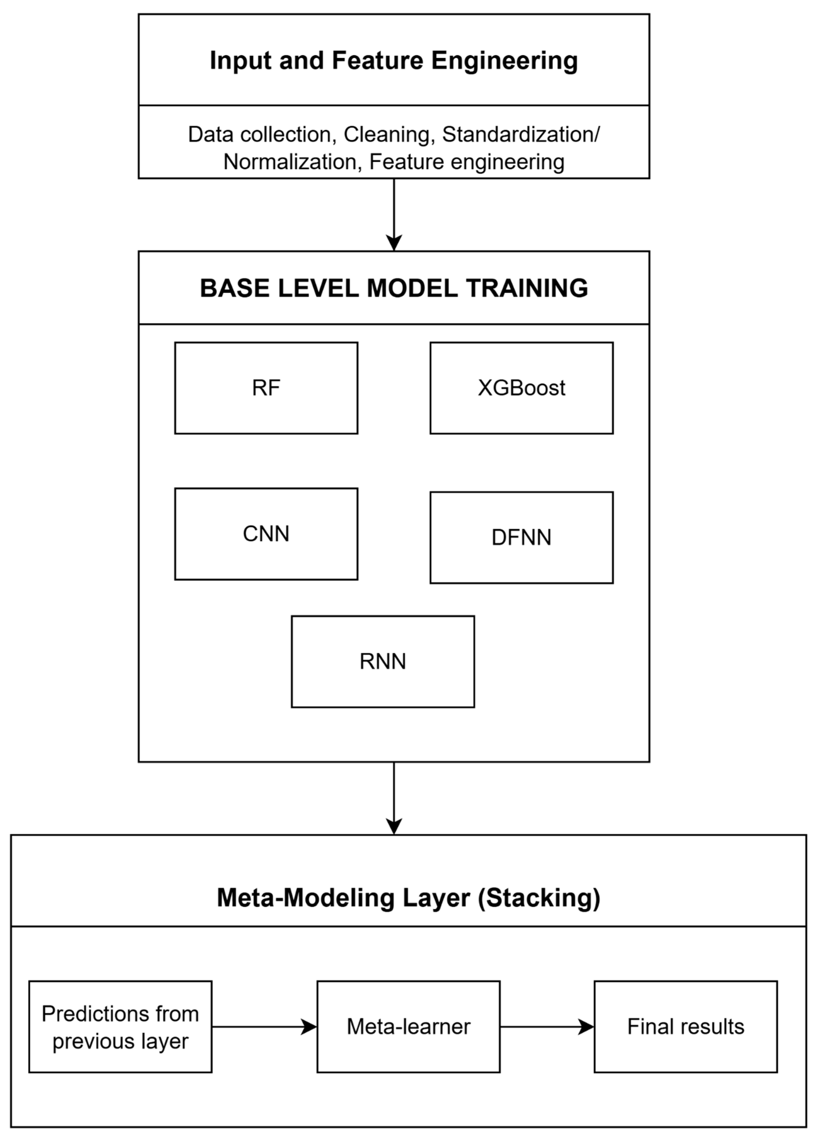
Figure 1. The methodology of the proposed Hybrid Meta-Ensemble framework.
Computers 14 00499 g001
Figure 2. Physiographic map of Potwar Basin regional framework displaying various physiographic features and topographic variations. The basin is divided into three major plateaus, including Northern Potwar, Southern Potwar, and Eastern Potwar comprising various plateaus, valleys, piedmonts, and mountain ranges, hosting several producing hydrocarbons fields [24].
Computers 14 00499 g002
Figure 3. Input well log data and compute petrophysical properties of the Qazian 1X well. The dataset is further utilized in pore pressure prediction though machine learning. The data displayed in the logplot view includes gamma ray (GR) curve in track 1; volume of shale (Vsh) in track 2; sonic transit time (DT) and normal compaction trendline (NCT) in track 3; resistivity in track 4; and pressure profiles including hydrostatic pressure (HP), overburden pressure (OB), pore pressure (PP), and DST data in track 5.
Computers 14 00499 g003
Figure 4. Input well log data and computed petrophysical properties of the Missa Keswal-01 well. The data displayed in the logplot view includes GR in track 1; Vsh in track 2; DT and NCT in track 3; resistivity in track 4; and pressure profiles including HP, OB, PP, and DST data in track 5.
Computers 14 00499 g004
Figure 5. Input well log data and computed petrophysical properties of Missa Keswal-03 well. The data displayed in the logplot view includes GR in track 1; Vsh in track 2; DT and NCT in track 3; resistivity in track 4; and pressure profiles including HP, OB, and PP in track 5.
Computers 14 00499 g005
Figure 6. Scatter plots comparing actual versus predicted pore pressure (in psi) for six machine learning models (CNN, DFNN, RNN, Random Forest, XGBoost, and Meta-Model Stacking), with diagonal reference lines indicating perfect prediction and performance metrics (R2 and RMSE) displayed for each model. The dashed line shows the ideal 1:1 correspondence between actual and predicted values.
Computers 14 00499 g006
Figure 7. Residual analysis plots showing predicted pore pressure versus residuals (in psi) for six models (CNN, DFNN, RNN, Random Forest, XGBoost, and Meta-Model) with overlaid moving average trends (green lines) and performance metrics (ρ values). Red dashed lines indicate standard deviation of the residuals.
Computers 14 00499 g007
Figure 8. Model performance by depth intervals showing R2 values at shallow (1150–1350 m), medium (1350–1550 m), and deep (1550–1700 m) sections for CNN, DFNN, RNN, Random Forest, XGBoost, and Meta-Model.
Computers 14 00499 g008
Figure 9. Model performance comparison on blind well validation set displaying R2 scores across train, validation, and test sets for all six models.
Computers 14 00499 g009
Figure 10. Model prediction correlation matrix showing pairwise correlation coefficients between predictions from CNN, DFNN, RNN, Random Forest, XGBoost, and Meta-Model.
Computers 14 00499 g010
Figure 11. Performance comparison of RF and XGBoost model without versus with 15% blind well data in training, showing scatter plots of actual versus predicted pore pressure for original RF (R2 = −1.229) and augmented RF (R2 = 0.888) followed by original XGBoost (R2 = −1.004) and augmented XGBoost (R2 = 0.935).
Computers 14 00499 g011
Figure 12. Error distribution histograms for Random Forest and XGBoost models comparing original versus augmented versions, showing improved prediction accuracy with reduced error spread after augmentation.
Computers 14 00499 g012
Figure 13. Composite logplot of the Missa Keswal-02 well displaying petrophysical properties and pressure profiles across key stratigraphic interval, including GR based lithology variations, volume of shale (Vsh), sonic transit time (DT) with normal compaction trend (NCT), porosity (SPHI), and pressure curves (HP, OB, PP, and predicted pressure).
Computers 14 00499 g013
Table 1. Equations used for the calculation of petrophysical properties.
PropertyFormulaParameters Description
Gamma Ray IndexEquation (1)   I G R = G R l o g     G R m i n G R m a x       G R m i n IGR = gamma ray index
GRlog = GR log value
GRmin = GR minimum value
GRmax = GR maximum value
Shale Volume
(Steiber Correction)
Equation (2)   V s h = 0.5 I G R 1.5     I G R Vsh = volume of shale
Density PorosityEquation (3)   P H I D = ρ m a     ρ b ρ m a     ρ f PHID = density porosity
ρma = matrix density
ρf = drilling fluid density
ρb = bulk density
PorosityEquation (4)   P H I S = D T     D T m a   D T f     D T m a   PHIS = sonic porosity
DTma = matrix transit time
DTf = drilling fluid transit time
DT = transit time from sonic log
Hydrostatic PressureEquation (5)   H P =   0 z ρ f × g   × d z HP = hydrostatic pressure
g = gravity acceleration
z = depth
Overburden Pressure Equation (6)   O B =   0 z ρ b × g   × d z OB = overburden pressure
Pore PressureEquation (7)   P P = O B O B   H P × N C T D T 3 PP = Pore Pressure
Table 2. Performance comparison of base models before and after fine-tuning on blind well test data.
ModelConfigurationR2RMSE (psi)MAE (psi)RelRMSE (%)
CNNOriginal−1.03551155.62915.8429.09
Fine-tuned0.7692389.13294.3210.03
RNNOriginal−0.81631091.64874.4627.47
Fine-tuned0.7712387.45287.759.50
DFNNOriginal−1.32601235.35928.6631.09
Fine-tuned0.7878373.11280.379.34
RFOriginal−1.22941209.40976.9730.44
Fine-tuned0.8883270.77179.666.81
XGBoostOriginal−1.00371146.55928.3628.86
Fine-tuned0.9350206.46147.125.20
Table 3. Performance comparison of meta-ensemble methods on blind well test data.
Ensemble MethodR2MAERMSERelRMSE (%)
Simple Average0.8645219.83298.217.51
Weighted Average0.8711213.82290.857.32
Stacking0.9382140.05201.25.07
Table 4. Leave-One-Well-Out Cross-Validation results.
ModelMean R2Std DevRMSE (psi)MAE (psi)
Meta-Model0.959±0.031142.482
XGBoost0.947±0.03414584.4
Random Forest0.944±0.058159.389.8
CNN0.833±0.118299.3215.1
DFNN0.833±0.115298.3214.7
RNN0.825±0.114310.8218.8
Disclaimer/Publisher’s Note: The statements, opinions and data contained in all publications are solely those of the individual author(s) and contributor(s) and not of MDPI and/or the editor(s). MDPI and/or the editor(s) disclaim responsibility for any injury to people or property resulting from any ideas, methods, instructions or products referred to in the content.