An Embedded Convolutional Neural Network Model for Potato Plant Disease Classification

Abstract

Globally, potatoes are one of the major crops that significantly contribute to food security; hence, the field of machine learning has opened the gate for many advances in plant disease detection. For real-time agricultural applications, it has been found that real-time data processing is challenging; this is due to the limitations and constraints imposed by hardware platforms. However, such challenges can be handled by deploying simple and optimized AI models serving the need of accurate data classification while taking into consideration hardware resource limitations. Hence, the purpose of this study is to implement a customized and optimized convolutional neural network model for deployment on hardware platforms to classify both potato early blight and potato late blight diseases. Lastly, a thorough comparison between both embedded and PC simulation implementations was conducted for the three models: the implemented CNN model, VGG16, and ResNet50. Raspberry Pi3 was chosen for the embedded implementation in the intermediate stage and NVIDIA Jetson Nano was chosen for the final stage. The suggested model significantly outperformed both the VGG16 and ResNet50 CNNs, as evidenced by the inference time, number of FLOPs, and CPU data usage, with an accuracy of 95% on predicting unseen data.

1. Introduction

It is believed that the hydrological cycle has been seriously altered by rising sea levels, the change in precipitation patterns, and the temperature increase caused by climate change. Such circumstances can aggressively impact human health, the economy, and agriculture [1]. On the other hand, preserving the vital role of soil as a support for vegetation and a source of nutrients requires an effective management approach for soil fertility [2]. The agricultural sector contributes significantly to the Egyptian economy with a growth rate of 3.2%, in addition to employing 25.6% of the total population. The effective collaboration of both agricultural extension and farmers can help in increasing farmers’ productivity in addition to raising rural families’ living standards by acquiring new skills and sufficient agricultural knowledge [3].

It is believed that direct yield losses caused by weeds, animals, and pathogens can range from 20% to 40%. To reduce such losses, plant pathologists have to acquire more knowledge from other scientists who address this issue [4]. On considering yield losses resulting from plant diseases, effective control measures should be implemented through advanced detection and correct identification of pathogens. Visual observation of plants’ symptoms is used as an initial step to identify different plant diseases. This method can provide some insights; however, true symptom identification will always be a challenge to address. Visual observation has its limitations in providing information related to the stage of infection or causative agent. Hence, adopting more standardized and advanced techniques for pathogen detection and identification is important. This could possibly guarantee a more accurate, reliable, and precise diagnosis of plant diseases.

Remote sensing, molecular diagnostics, imaging technologies, big data analytics, and machine learning are considered some of the recent powerful advancements for early and precise detection of plant diseases [5]. Nowadays, machine learning plays a vital role in analyzing complex datasets; this can provide an innovative solution to achieving high accuracy in disease detection in addition to accurate identification of disease severity [6].

It is important to mention that convolutional neural networks (CNNs) are machine learning models specifically used for addressing classification problems. CNNs extend original artificial neural networks (ANNs) by adding more depth and convolutions to the network; that is why it is called deep learning. The main reason behind the motivation for using CNNs is the fact that, recently, the agricultural field has heavily relied on machine learning, especially convolutional neural networks. Multiple research efforts have used CNNs to address many agricultural challenges. This technology can pave the way for adopting new imaging techniques for automatic plant disease diagnosis. This can greatly assist farmers in developing more advanced farming techniques and efficient agricultural practices to help in maintaining food security [7].

The field of machine learning has opened the gate to endless possibilities, allowing for significant promotion of various industries. Yet, this field is still facing many challenges, one of which is its inability to interact directly with the physical world. In this stage, the significant role of embedded AI has come to light, serving as the bridge through which machine learning is allowed to interact with and influence the real world.

By embedding machine learning into edge devices such as smart home gadgets, smart phones, or industrial machines, there is now a capability to process information on the spot. Devices making smart and reliable decisions lead to the autonomous completion of complex tasks without the need for continuous internet access or devices being hindered by delays in cloud computing applications.

Recently, the rise of edge computing has fundamentally refined the landscape of data processing, as it marks an important moment in the evolution of digital infrastructure. Shifting towards edge computing is a crucial move as it represents modern technology shifting away from the dominant centralized, cloud-centric models, addressing the great need for real-time computing power closer to data generation sources. Influenced by this direction, to release the full potential of edge big data, artificial intelligence must be pushed to the edge of the network. This is what caused the rise of the edge computing paradigm, which pushes data processing similar to providing services or complex computing tasks from the network core to the network edge [8]. The core of edge computing is mainly minimizing latency and providing localized data processing capabilities, opening the gate for faster and more efficient decision making in critical tasks for various fields. The integration between edge computing and embedded AI is currently shaping a new era of efficient, fast, and real-time data processing. This relationship introduces an innovative solution for edge devices where it is possible to analyze data and make autonomous, smarter, and reliable decisions without relying on constant connectivity to the cloud [9].

Due to the consistent need for higher computing and memory capabilities, it is always important to consider the limitations imposed by edge devices. That is why optimization is performed for neural network models to address these limitations.

In this study, the main aim is to develop an optimized and customized convolutional neural network model that can be easily deployed on hardware platforms while maintaining a balance between consuming minimum hardware resources and high model performance. The focus in this study is on the detection and classification of potato diseases, particularly potato early blight and potato late blight. The developed model remarkably outperformed VGG16 and ResNet50 CNNs, maintaining a robust balance between high accuracy in unseen data classification and embedded deployment for real-time precision agriculture applications.

The rest of this paper is organized as follows: Section 2 provides a survey of the related work; Section 3 details the adopted methodology, followed by the results and discussions in Section 4 and Section 5, respectively. Finally, Section 6 concludes this paper.

2. Related Work

Nowadays, the digital age has widely opened its gate to many precision-agricultural applications where data are becoming not just valuable but also smart [10]. In addition to crop disease detection, disease classification is necessary for applying proper control actions. However, detection and classification of crop diseases using patterns in images are sometimes challenging. That is why convolutional neural networks are used; they are a type of deep learning network that is capable of extracting features from images, thus making disease identification feasible and more reliable [7]. A critical point to note is the following: if the information perceived from all farmlands is gathered into the cloud server, this would put intense pressure on the server processing these data, causing the network response to become extremely slow in event processing. This issue can be perfectly solved if edge computing was taken into consideration [8]. Edge computing can effectively address the concerns of bandwidth cost savings, battery life constraints, response time requirements, data privacy, and safety [11].

Some studies focused only on the software/PC implementation of neural network models while conducting performance analysis of the models. However, other research efforts focused on the embedded implementation of neural networks to overcome the network delay and achieve efficient real-time response for smart decision-making applications.

A study used the PlantVillage dataset and focused on employing Google LeNet and AlexNet. The trained deep learning model achieved a sustained testing accuracy of 99.35% [12]. A reasonable success rate was achieved by another study that used Alex NetOWTB and VGG. This research achieved the best performance of 99.53% [13]. According to a different study, the accuracy of a model that used the VGG16 CNN was 97.22% for rice plant leaf disease detection and reached an accuracy of 98.75% for identification of wheat plant leaf diseases [14]. In [15], the authors used AlexNet and GoogleNet to detect nine diseases of tomatoes. The researchers reached an accuracy of 99.18% for the GoogleNet CNN model. In a different study, the authors prioritized utilizing unmanned aerial vehicles (UAVs) in tasks related to crop management and monitoring. They proposed a computerized system, selecting the convolutional neural network as an identification tool for high-accuracy detection of Fusarium wilt of Radish. For the classification process, the convolutional neural network achieved an accuracy of 93.3% [16]. Another study used the VGG16 CNN model. The detection process was used to handle nineteen different classes of plant diseases. The authors of this study achieved an accuracy of 95.2%, in addition to the testing loss that was about 0.4418 [17]. For further applications of deep learning, the study aimed to use the technology of deep learning in identifying external defects of tomatoes. The ResNet50 deep learning classifier was chosen in this study. After training, the model detected external defects in tomatoes using fine-tuning and feature extraction. On average, the model achieved a precision of 94% on the testing set. It is crucial to note that the key to model success lies within its almost ideal identification of healthy plant images, which is addressed in this study [18]. In [19], the authors proposed a custom lightweight model, in addition to utilizing transfer learning models, specifically VGG-16 and VGG-19, for the purpose of detecting tomato diseases that infect plants leaves. By applying techniques of data augmentation, the proposed model achieved the highest classification accuracy and a recall of 95% compared to the other transfer learning-based models. Finally, a Web-based and Android-based end-to-end (E2E) system was developed that utilized the implemented model to further assist farmers in classifying tomato plant leaf diseases.

For the detection of powdery mildew, optimization and evaluation were performed on several convolutional neural network models that were used as disease classification tools. The study focused on ResNet-50, SqueezeNet, SqueezeNet-MOD1, SqueezeNet-MOD2, AlexNet, and GoogleNet CNN models. All the used deep learning models accredited in this study showed an average classification accuracy of more than 92%. The ResNet50 model provided the highest disease classification accuracy of 98.11%. AlexNet CNN had the least computation time of only 40.73 s, used to process 2320 images with a classification accuracy of 95.59%. Finally, for hardware deployment, SqueezeNet-MOD2 CNN consumed the least hardware resources considering the memory requirements, with a classification accuracy of 92.61% in detecting both diseased and healthy images [20]. In another study, training and evaluation of various deep learning classifiers are presented for the classification of plant leaf diseases. Four convolutional neural networks were chosen, dedicated to classifying tomato leaf diseases. Finally, a hardware implementation was developed for the selected CNN models on the Raspberry Pi 4 microcomputer with a graphical user interface. The results showed that the Xception model achieved an accuracy of 100% with 2512 s (about 42 min) per epoch during the training process [21]. In [22], the main target was to integrate the Jetson Nano machine with a pretrained convolutional neural network dedicated to the detection of diseased and healthy plant images. A video server was created that uses the real-time streaming (RTSP) protocol for sending video data to the detection engine. At an adjustable frequency, the host-detected diseases are then sent through the simple mail transfer protocol (SMTP) to the users’ emails.

In the field of agriculture, the implemented system can greatly help, making overcoming plant diseases more effective and profitable. After training for 50 epochs, the artificial intelligence algorithm achieved its best accuracy on epoch 15, with a training accuracy of 98.7%. Another study built a custom convolutional neural network that has been trained on Google Colab using diseased and healthy plant images. The trained model is evaluated using different single-board computers (SBCs) that include different essential characteristics, focusing on Raspberry Pi 3, Raspberry Pi 4, NVIDIA Graphic Processing Units, and Tensor Processing Unit (TPU) processing units carried by the Google Coral Dev TPU Board devices to execute custom CNN models with the aim of detecting various plant diseases. On evaluating the performance of the application, the deep learning model showed remarkable results as it achieved a classification accuracy of 90% [23].

For the purpose of accurate classification, various recent advancements in this domain focus mainly on complex and deep neural network architectures. Despite their impressive performance, such models consume substantial hardware resources such as processing power and memory. This makes real-time embedded deployment for these models impractical in most cases. Hence, there has been a growing need for lightweight and computationally efficient CNN architectures. Some researchers used fine-tuning or data augmentation to enhance the classification accuracy of their models. Unfortunately, such techniques do not contribute to the depth of the networks or even resolve the high-complexity problem of the CNN models. Hardware deployment has its own resource restrictions and constraints; hence, to achieve success in hardware implementation of convolutional neural networks, preserving the simplicity of the model is a must, while maintaining high accuracy in classification. Such a trade-off is not easy; that is why optimization is needed. Performing model optimization is better than model compression for various reasons including accuracy preservation, model flexibility, and hardware deployment. Accordingly, an optimized CNN model is developed in this study that efficiently utilizes hardware resources while maintaining high accuracy and reliability in detecting and classifying potato plant diseases. To advance precision agriculture, the main goal of this paper is intended to develop a customized CNN model that should feature flexible architecture, hence allowing for future enhancements and adaptation to different evolving field requirements.

3. Materials and Methods

Potatoes are grown on a significant scale in more than one hundred and thirty countries. In 2016, the gross production of potatoes reached a value of 63.6 billion US dollars, with an annual potato production of 368 million tons in 2018. Potatoes are now grown for several reasons, such as food, industrial uses, exporting, and animal feed [24]. Since the 1960s, it is believed that the production of potatoes has enormously increased in developing countries [25]. Among all crops grown in Egypt, potatoes are one of the most important crops for many purposes, including food and industry. Unfortunately, recent studies have shown that the amount of potato production is declining, where the exported amount in Egypt has decreased from 808.2 thousand tons in 2017 to 561.4 thousand tons in 2020 due to the COVID-19 pandemic. This yield loss is reflected in the availability of the hard currency as well as the balance of payments [26]. Because of the vegetative propagation of all varieties of potatoes by tubers, they are intensively subjected to various types of pathogenic organisms. Such pathogens may be viruses, fungi, or bacteria, causing losses while growing, harvesting, or even at tuber storage. The list of pathogens infecting potatoes remains unchanged over decades [27], drastically affecting yield production, causing degradation in both quality and quantity of the potato crop.

Hence, to tackle agricultural challenges, artificial intelligence uses robots, deep learning, image processing, artificial neural networks, Internet of Things (IoT), and other cutting-edge methods. Without a doubt, all these technologies can assist farmers in the real-time monitoring of various items obtained from their farms, such as water usage, weather, soil conditions, and temperature [28].

3.1. Potato Plant Diseases

The most common pathological diseases infecting potato leaves are early blight and late blight. Over the years, the world has witnessed their significant effect on yield, causing severe losses worldwide. Hence, many studies are being conducted for addressing challenges caused by these plant diseases.

In 1882, the symptoms of early blight were observed for the first time on dying potato leaves. The name early blight came from the fact that it severely infects early maturing cultivars more than medium or late maturing cultivars. At the beginning, the infected leaves show dark brown dot-like circular, oval, or angular blotches a few millimeters in diameter. The spots may cluster and enlarge until forming a large necrotic area. This area can gradually expand, and the symptoms on leaves can grow until taking up the whole of the green tissue. As the lesions start to grow, a series of concentric dark rings are visible, caused by the pathogen’s irregular growth patterns. The symptoms of early blight are typically characterized by a target-spot or bull’s eye pattern, as represented in Figure 1a. Depending on the geographical regions and cultivar susceptibility, early blight can cause severe damage to potato yield, and such damage can range from 2% to 58%. In India, the recorded losses in severe conditions due to early blight damage have been estimated up to 79% [29]. Another research study stated that such a disease can cause damage to both potato tubers and foliage. Due to the early blight effect, yield losses in different regions vary enormously from 5% to 78% [30].

Late blight disease was first discovered in the mid-nineteenth century; it played a drastic role in the Irish potato famine in the 1840s [31]. The foliage infection of this disease appears mostly near the margins and tips of leaves. It emerges as water-soaked irregular pale green lesions that quickly grow into large necrotic spots that are brown to purplish black in color. On the lower surface of the infected leaves, a white mildew that consists of spores and sporangia of the disease pathogen can be clearly recognized, particularly around the edges of the necrotic lesions. Light to dark brown lesions surround the plant stem and petioles, making the plant weak at such locations; hence, crop collapse becomes possible. Under favorable disease conditions, the entire infected crop gives a blackened, blighted appearance with a chance of plant destruction within a week, and potato late blight is clearly illustrated in Figure 1b [32]. The recorded losses due to potato late blight reached 16% of total global production. Due to late blight, losses in yield ranged from 20% to 70%. Such a disease can destroy the entire potato crop under epidemic conditions [29]. In Ethiopia, the estimated potato crop losses due to late blight ranged from 22% to 46%. This disease causes severe losses in yield, in addition to reducing its marketability value [33]. For additional demonstration, the healthy potato leaf is represented in Figure 1c.

3.2. Convolutional Neural Networks

Convolutional neural networks, referred to as CNNs or ConvNets, are a special type of deep neural network dedicated mainly to analyzing input data that contain some spatial structure. They were initially introduced to address computer vision-related problems, for example, robotics, security, medical diagnoses, and self-driving cars, by using images as the main source of data.

First, CNNs work by retrieving low-level representations, such as points and local edges, and then composing higher-level representations similar to contours and overall shapes. The name convolutional neural network came from the fact that such networks perform convolutions. Convolution operations are a type of linear mathematical operation that is used in at least one of the hidden layers via CNNs. On comparing CNNs to other classification algorithms, the required preprocessing in a CNN is much lower. In this type of network, there is no need to explicitly define which input samples should be selected from the analysis, since CNNs optimize a complete end-to-end process that is performed to ideally map data samples to outputs, which are consistent with the labeled data samples used in the training process of the deep learning algorithm.

By using many layers of filters, CNNs are now considered a powerful and reliable tool for the analysis of images [34]. With convolutional neural networks becoming more of a commodity in the field of computer vision, various attempts have been made to improve the original traditional architectures to achieve better performance [35].

Consequently, this results in significantly more accurate network architectures, for example, VGG16 and ResNet50 CNNs. Their popularity was acquired from their significant performance, as the VGG16 CNN is very appealing with almost 134 million parameters [36]. This is due to its stable behavior and uniform architecture [37,38]. Similarly, the ResNet50 CNN is extremely popular with almost 23 million parameters [36], and its popularity is due to the residual blocks that ease the process of learning. One main advantage of the ResNet50 CNN over the other neural networks is its ability to train very deep neural networks. By using residual blocks and skip connections, it is possible to accelerate the training process as well as retain the relevant information learned in the earlier layers [39], hence solving the vanishing gradient problem and improving the performance of deep neural networks [40].

3.3. Dataset

The main aim of this study is to detect diseases that specifically infect potato leaves; hence, the adopted dataset holds three potato plant leave diseases. The first class contains images of potato leaves infected with early blight; the second class includes images of potato leaves infected with late blight; and the third class holds images of healthy potato leaves. The dataset was obtained from Kaggle [41] in 2020. The adopted dataset with its training, validation, and testing sets holds 14,256 images, with 7984 images in the training set, 2852 in the validation set, and 3420 images in the testing set; all images are of size 256 × 256 × 3. This splitting approach follows the 60/40 criteria, which is widely adopted in this field. This works by employing 60% of the dataset images in the training set, while the remaining 40% goes to the validation and testing sets, by assigning 20% to the validation set and 20% to the testing set.

3.4. Model Hyperparameters

Various metrics were chosen for optimizing the developed CNN model. These metrics included the model optimizer, the activation function, the loss function, the batch size, the kernel size, the number of filters, the number of epochs, and finally the learning rate. Choosing the right hyperparameters can greatly contribute to evolving the performance of the CNN model. Hence, this section includes a deep analysis of the optimization process that was performed and the hypothesis behind adopting the needed hyperparameters.

Regarding the optimizer, Adam, Adamax, and stochastic gradient descent (SGD) were specifically selected. Choosing a suitable optimizer in deep neural networks can significantly impact the accuracy of the model [42]. One of the most popular optimizers for training convolutional neural networks is stochastic gradient descent (SGD). Despite its efficiency and simplicity, this optimizer suffers from low convergence speed. This issue was avoided using the Adam optimizer, which practically achieved much faster convergence speed than the SGD optimizer [43]. Adam is an adaptive deep learning algorithm that has been broadly used in a variety of applications. Despite its speed in the training phase, its generalization performance is worse than that of the SGD optimizer, leading to poor class predictions in the testing dataset. Tuning Adam’s inner hyperparameters can help in raising the optimizer’s performance and narrowing the gap between SGD and Adam. However, this solution makes using Adam in deep learning models computationally expensive [43]. Sometimes, for embedded applications, Adamax is considered better than Adam Optimizer. The Adamax optimizer is represented as an alteration of Adam. It is built on the adaptive approximation of low-order moments. Despite fast convergence behavior, these adaptive algorithms such as Adam and Adamax suffer from worse generalization behavior than stochastic gradient descent (SGD) optimizers. Particularly, adaptive gradient algorithms often show effective progress in the faster training phase, but unfortunately, their performance is poor regarding test data prediction. On the other hand, practically, stochastic gradient descent usually improves the deep learning model performance slowly; however, it is capable of achieving higher performance when it comes to providing predictions in the given test set. An empirical explanation for this performance gap between adaptive optimizers and SGD is that adaptive gradient algorithms such as Adam and Adamax tend to converge to sharp minima whose local basin has quite a large curvature, and this can lead to poor generalization, while the SGD optimizer prefers to find flat minima, and that is why it generalizes better. By analyzing the optimizer’s escape time for the same basin, it is proved that SGD has a smaller escape time than adaptive optimizers do, and this explains its better generalization performance, leading to a more accurate prediction on a given testing set [43]. Based on the experimental results of the developed model testing accuracy, the SGD optimizer showed better performance compared to both Adam and Adamax.

Regarding the activation function, the ReLU activation function was chosen as a default in the inner CNN layers. Regarding the activation function in the output layer, the SoftMax activation function was the best choice. The main benefit of using activation functions is that they provide good capability of handling multiple classes in class classification problems. In this work, as mentioned earlier, SoftMax was the adopted activation function in the output layer of the implemented 2-CONV-Layer model. In CNN models, the SoftMax activation function is implemented just before the output layer, where it assigns decimal probabilities to each class that eventually add up to 1.0. It is a widely used activation function specifically in multiclass problems, as it maps the value of the output layer to a probability distribution over the different classes of the convolutional neural network. This probabilistic interpretation makes the interpretation of the network output much easier where the class with the highest probability is identified as the network’s final output. Equations (1) and (2) represent the mathematical representations of the utilized ReLU and Softmax activation functions. Simply, Equation (1) keeps all positive values unchanged while changing all negative values to 0. Equation (2) represents the mathematical formula for the Softmax activation function, where $p_i$ represents the predicted probability for class i, N is the total number of classes, and $a_i$ is the raw output for class i [44].

$$\mathrm{R}\mathrm{e}\mathrm{L}\mathrm{U}\left(z\right)=\left\{\begin{array}{c}0\hspace{1em}\hspace{1em}z<0\\ z\hspace{1em}\hspace{1em}z\ge 0\end{array}\right.$$

(1)

$$p_i={\displaystyle \frac{e^{a_i}}{\sum _{k=1}^N{e}^{a_k}}}$$

(2)

Regarding the CNN loss function, in convolutional neural networks, loss functions are typically used to evaluate the performance of models, concerning classification tasks in particular. The most commonly used loss function in CNNs is cross-entropy. It mainly has two types, Binary Cross-Entropy and Multiclass Cross-Entropy, which can also be called categorical cross-entropy loss or Softmax loss. The categorical cross-entropy loss function is crucial in machine learning applications [45]. It is widely used in training neural network models for multiclass classification problems. For a specified dataset with N instances, categorical cross-entropy loss (L) is calculated using Equation (3) [46], where C is the number of classes, p_i,j is the predicted probability for class j for instance i, and y_i,j are the true labels for class j for instance i.

$$L = -{\displaystyle \frac{1}{N}}{\sum }_{i=1}^N{\sum }_{j=1}^C(y_{i,j}·\mathrm{l}\mathrm{o}\mathrm{g}(p_{i,j}\left)\right)$$

(3)

Regarding the batch size, in this study, batch sizes of 32, 64, and 128 were chosen. Practically, it is always better to initially choose smaller batch sizes (e.g., 32 or 64). It is believed that in most cases, the batch sizes should always be a power of two. Many researchers suggested using the batch size of 32 as an effective default [47]. In the experiments performed in this study, the batch size of 32 provided the best CNN results, proving its efficiency in practical terms.

Regarding the number of filters, mostly, this value is chosen to be a power of two. In this study, the selected number of filters in the convolutional layers is 32, all of which are 3 × 3 in size for maintaining simplicity and lowering the computational complexity of the implemented CNN model. This choice of kernel size and number of filters is commonly used in various convolutional neural network implementations.

Finally, regarding the number of epochs, the experiments were initiated with a small number of epochs in the training phase; then, to enhance the network performance, the number of epochs was raised to twelve in the training phase. During experimentation, based on the empirical observation of model convergence, twelve epochs was selected for model training. On reaching the tenth epoch, the model showed stable performance specifically for the validation accuracy and loss curves, which demonstrated minimal improvement thereafter. Beyond the twelfth epoch, the model indicated the onset of overfitting as validation loss began to slightly increase. On setting the number of epochs to twelve during the training phase, it was ensured that the implemented CNN model was sufficiently trained to achieve optimal generalization while avoiding unnecessary and excessive computations, hence guaranteeing both a sufficient and balanced setting for training the implemented model in an effective manner while avoiding excessive computational complexity.

In addition, the default learning rate for the chosen optimizer was adopted. For the chosen SGD optimizer, the learning rate for the developed model is 0.01.

To summarize, several steps were used in the proposed methodology, including designing the model architecture, model optimization in choosing the appropriate hyperparameters, and finally model training and testing.

Table 1. The hyperparameters of the proposed 2-CONV-Layer model.

Hyperparameters	Assigned Value
Classes	3
Epochs	12
Batch size	32
Learning rate	0.01
Optimizer	SGD
Activation function in the output layer Activation function in the hidden layers Loss Function	SoftMax ReLU Categorical Cross-Entropy
Number of filters in each Conv layer	32
Kernel size	3 × 3

shows all the adopted hyperparameters during the optimization process of the developed model.

3.5. Proposed Model Architecture

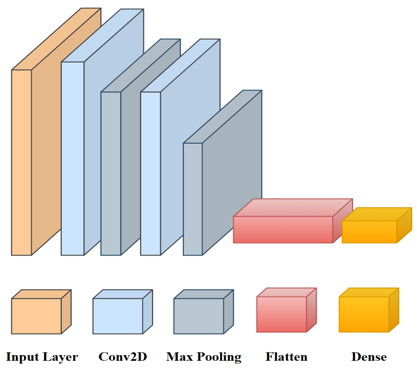
The proposed model consists mainly of two convolutional layers. The whole architecture is divided into two convolutional layers, two max pooling layers, one flatten layer, and one dense layer. During model implementation, only a 3 × 3 filter size is used for the kernels in all the convolutional layers for maintaining the simplicity in model structure. The exact structure of the proposed CNN architecture is described as follows: The first and second convolutional layers are composed of 32 feature kernel filters; each filter is of size 3 × 3. The input data is represented as a three-channel (RGB) image that is passed into the initial convolutional layer with dimensions 256 × 256 × 3. By passing the input image into the first convolutional layer, its dimensions will change to 254 × 254 × 32. Then, the resulting feature map will be passed to the max pooling layer with a stride of 2, which will result in a reduced feature map of size 127 × 127 × 32. The second layer is also a convolutional layer with 32 feature kernels; again, all filters are of size 3 × 3. The second convolutional layer is followed by another max pooling layer with a stride of 2, which results in a reduced feature map of size 62 × 62 × 32. Following that is a flatten layer, and a SoftMax classifier was finally chosen in the dense layer that represents the output layer of the implemented model. The whole architecture of the developed model is represented in Figure 2.

4. Results

The aim of this study was to develop a customized 2-Convolutional-Layer neural network for potato plant disease classification, and then to deploy the implemented model on two hardware platforms: Raspberry Pi 3 as an intermediate stage and NVIDIA Jetson Nano as a final stage. Due to resource limitations imposed by embedded devices, implementing an efficient and reliable model that suits the resource constraints was an extremely difficult trade-off. That is why model optimization was performed, to keep the model structure as simple and efficient as possible. After reaching the desired accuracy, the performance of the implemented model was compared against two well-known neural network models: VGG16 CNN [48] and ResNet50 CNN models [49].

4.1. PC Simulation Implementation

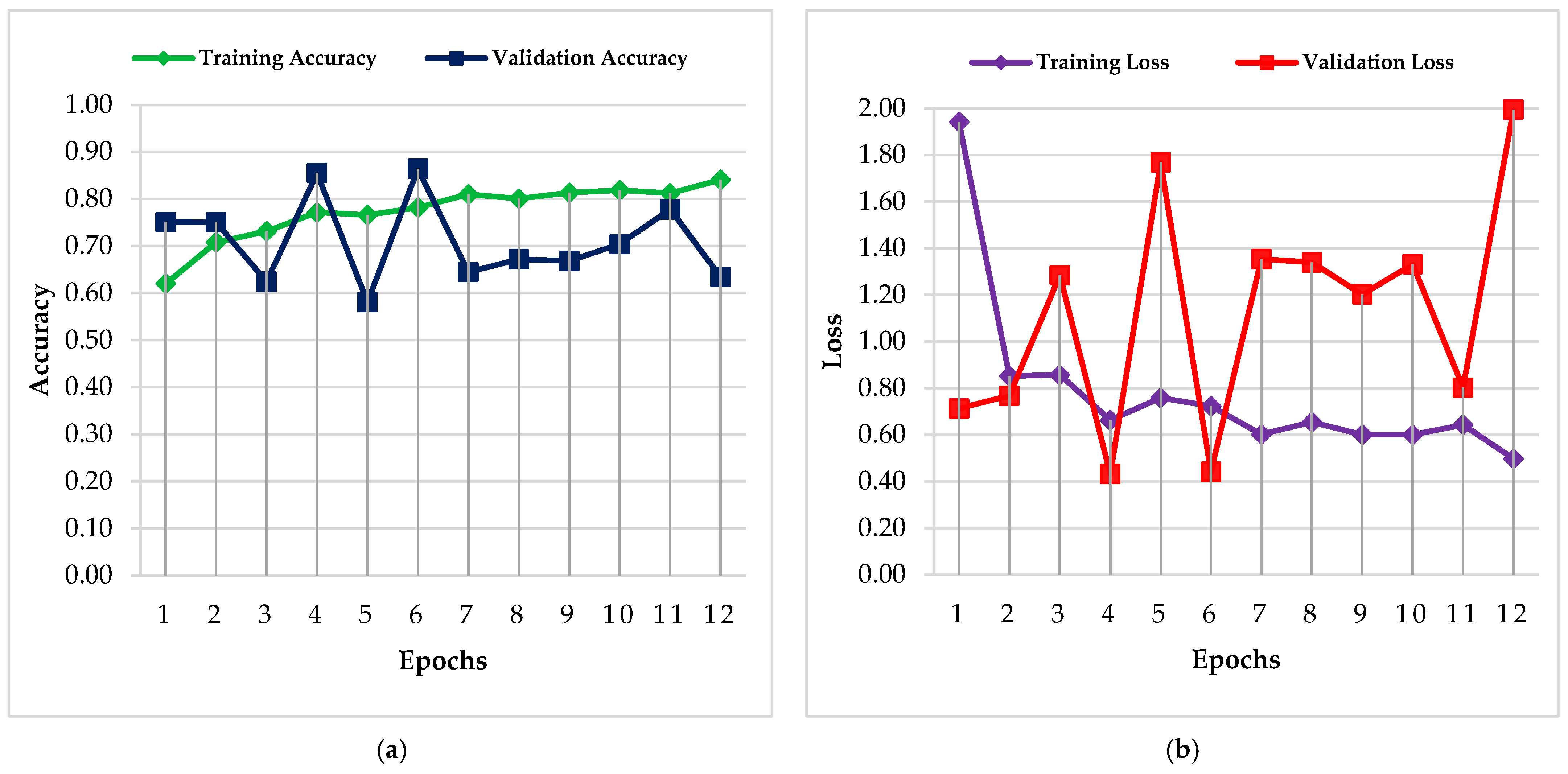
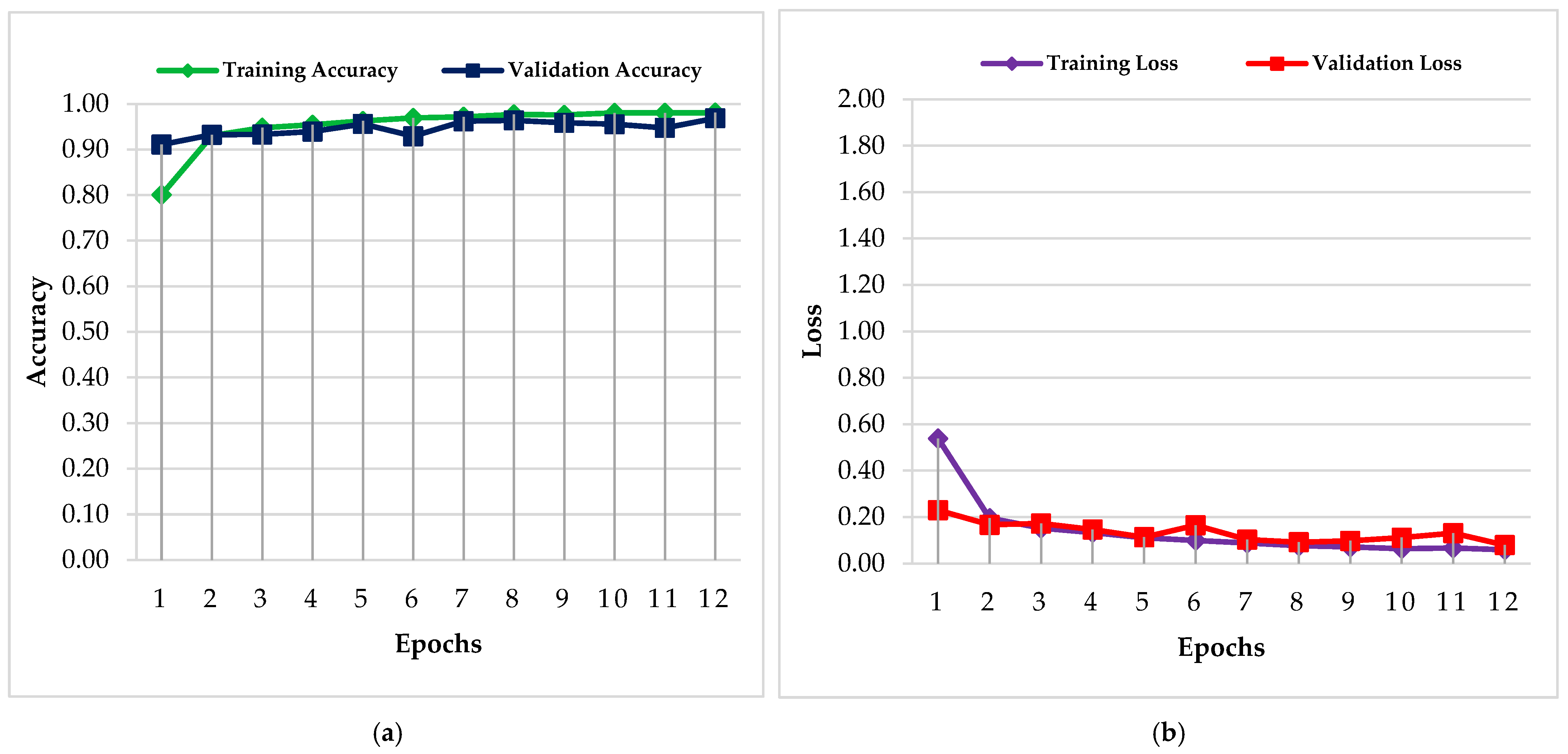
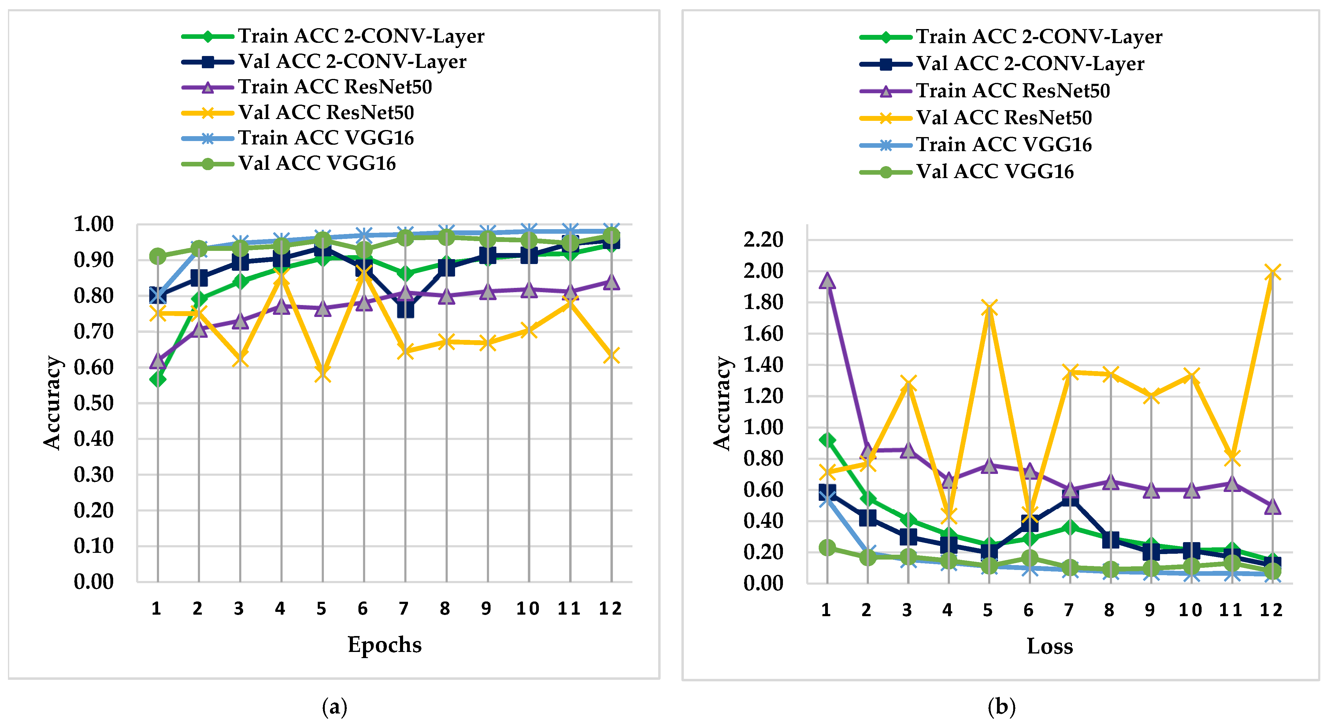
In the software implementation, the code was designed on an HP laptop with an Intel(R) Core(TM) i7-6820HQ CPU@2.70 GHz. The model was designed using the Jupyter notebook on Anaconda Navigator 3 with Python version 3.7. A thorough performance analysis was made between the developed model against both VGG16 and ResNet50 CNNs for twelve epochs in the training stage. In order to show the complete analysis of the three CNN models, both accuracies and losses concerning the training and validation phases for each model are clearly illustrated in Figure 3, Figure 4 and Figure 5, where (a) represents the model training and validation accuracy and (b) represents the model training and validation loss across the twelve epochs. Additionally, for clearly demonstrating the comparison between the performance of the three CNN models during simulation, Figure 6 clearly represents the accuracy and loss curves for training and validation of the models, where (a) represents the models’ training and validation accuracy and (b) represents the models’ training and validation loss.

As shown in the previous figures, it is obvious that both VGG16 and the 2-Convolutional-Layer models had considerably higher training and validation accuracies than the ResNet50 model did, in addition to lower loss values. The ResNet50 model was unstable regarding the validation for both accuracy and loss; this refers to the overfitting problem where the model learns its training data very well and behaves poorly on the validation data. Meanwhile, VGG16 had stable behavior through all the twelve epochs of the fitting stage. The developed 2-Convolutional-Layer model had a stable behavior with only one ripple at the seventh epoch. The stability of the developed model, in addition to its high accuracy and low loss value, can give clear insight into the superior performance on unseen data.

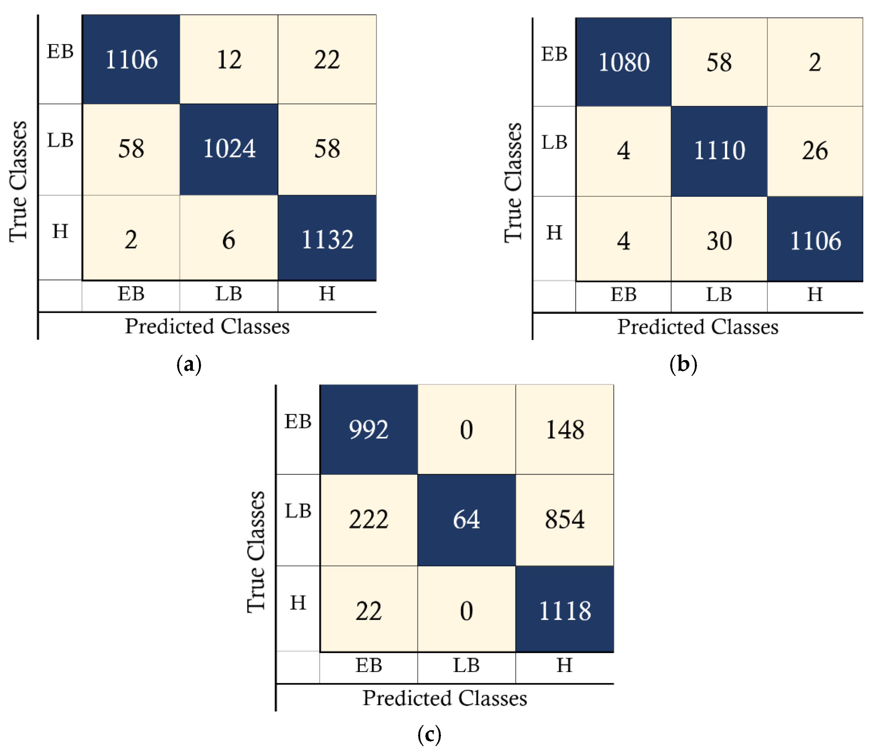
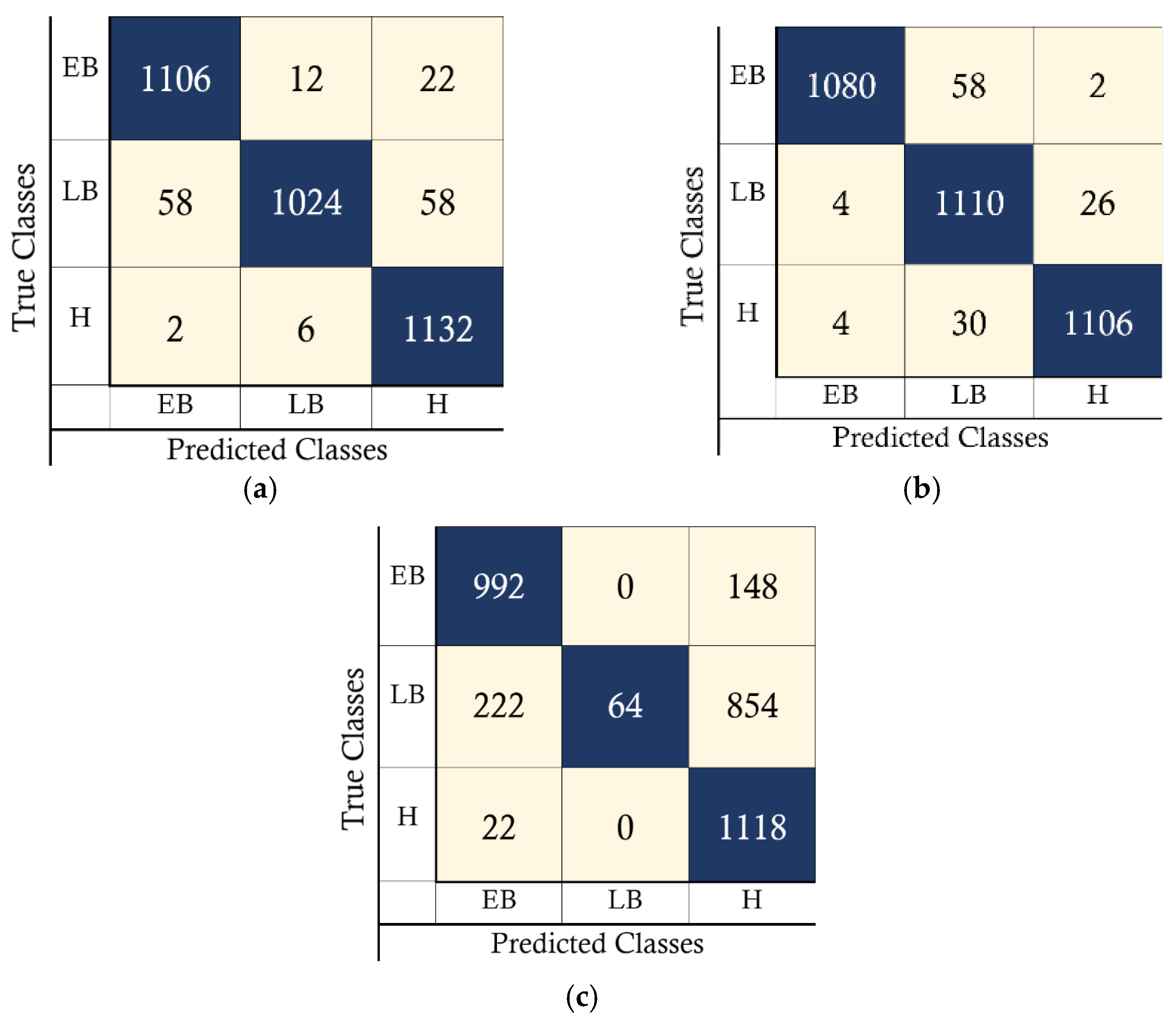
In addition, to clearly compare the efficiency and performance of the three models, some metrics were taken into consideration: Accuracy, Precision, Recall (Sensitivity), F1-score, Macro-F1, and Weighted-F1. The mathematical formulas used to compute these metrics are provided in Equations (4)–(9) [21], where TP, TN, FP, and FN refer to true positive, true negative, false positive, and false negative, respectively. These computations can only be performed after constructing the confusion matrix for each model for both PC and embedded implementations. The confusion matrices are clearly represented in Figure 7, Figure 8 and Figure 9.

The confusion matrix is used widely in machine learning for predictive analysis. C1, C2, and C3 refer to classes 1, 2, and 3 in the adopted testing dataset, respectively. In the comparisons illustrated in

Table 2. Performance metrics of the three CNN models for PC implementation.

Classes	Accuracy	Precision	Recall	F1-Score	Macro-F1
2-Convolutional-Layer CNN
EB	0.973	0.95	0.970	0.959	0.952
LB	0.960	0.982	0.896	0.937
H	0.973	0.930	0.992	0.960
VGG16 CNN
EB	0.983	0.994	0.954	0.973	0.966
LB	0.967	0.932	0.974	0.952
H	0.982	0.975	0.971	0.973
ResNet50 CNN
EB	0.880	0.790	0.873	0.829	0.545
LB	0.687	1.000	0.061	0.115
H	0.708	0.533	0.978	0.691

,

Table 3. Performance metrics of the three CNN models for Raspberry Pi 3 implementation.

Classes	Accuracy	Precision	Recall	F1-Score	Macro-F1
2-Convolutional-Layer CNN
EB	0.972	0.948	0.970	0.959	0.953
LB	0.960	0.982	0.898	0.938
H	0.974	0.933	0.992	0.962
VGG16 CNN
EB	0.980	0.992	0.947	0.969	0.963
LB	0.966	0.926	0.973	0.949
H	0.981	0.975	0.970	0.972
ResNet50 CNN
EB	0.885	0.802	0.870	0.834	0.542
LB	0.685	1.000	0.056	0.106
H	0.700	0.527	0.980	0.685

and

Table 4. Performance metrics of the three CNN models for NVIDIA Jetson Nano implementation.

Classes	Accuracy	Precision	Recall	F1-Score	Macro-F1
2-Convolutional-Layer CNN
EB	0.972	0.948	0.970	0.959	0.953
LB	0.960	0.982	0.898	0.938
H	0.974	0.933	0.992	0.962
VGG16 CNN
EB	0.980	0.992	0.947	0.969	0.963
LB	0.966	0.926	0.973	0.949
H	0.981	0.975	0.970	0.972
ResNet50 CNN
EB	0.885	0.802	0.870	0.834	0.542
LB	0.685	1.000	0.056	0.106
H	0.700	0.527	0.980	0.685

, the notations EB, LB, and H stand for early blight, late blight, and healthy leaves classes, respectively. In addition, the Weighted-F1 metric was not included in the comparison, because it was equal to the value of the F1-score metric. This is due to the utilization of a testing set with the same number of images in the three classes.

$$\mathrm{A}\mathrm{c}\mathrm{c}\mathrm{u}\mathrm{r}\mathrm{a}\mathrm{c}\mathrm{y}={\displaystyle \frac{TP+TN}{TP+TN+FP+FN }}$$

(4)

$$\mathrm{P}\mathrm{r}\mathrm{e}\mathrm{c}\mathrm{i}\mathrm{s}\mathrm{i}\mathrm{o}\mathrm{n}={\displaystyle \frac{TP}{TP+FP }}$$

(5)

$$\mathrm{R}\mathrm{e}\mathrm{c}\mathrm{a}\mathrm{l}\mathrm{l}={\displaystyle \frac{TP}{TP+FN }}$$

(6)

$${\mathrm{F}1}_{\mathrm{S}\mathrm{c}\mathrm{o}\mathrm{r}\mathrm{e}}={\displaystyle \frac{2\times Precision\times Recall}{TP+FN }}$$

(7)

$$\mathrm{M}\mathrm{a}\mathrm{c}\mathrm{r}\mathrm{o} {\mathrm{F}1}_{\mathrm{S}\mathrm{c}\mathrm{o}\mathrm{r}\mathrm{e}}={\displaystyle \frac{ {F1}_{Score\left(C1\right)}+{F1}_{Score\left(C2\right)}+{F1}_{Score\left(C3\right)}}{3}}$$

(8)

$$\mathrm{W}\mathrm{e}\mathrm{i}\mathrm{g}\mathrm{h}\mathrm{t}\mathrm{e}\mathrm{d} \mathrm{F}1={\displaystyle \frac{\left({imgs}_{\left(C1\right)}\right)·{F1}_{\left(C1\right)}+\left({imgs}_{\left(C2\right)}\right)·{F1}_{\left(C2\right)}+\left({imgs}_{\left(C3\right)}\right)·{F1}_{\left(C3\right)}}{Total number of images in testing set}}$$

(9)

4.2. Embedded Implementation

In this section, the comparison mainly includes the embedded implementations of the three CNN models on the Raspberry Pi 3 platform as an intermediate stage and then the NVIDIA Jetson Nano platform as a final stage. The main concern addressed in this study is the implementation of an efficient and reliable CNN model dedicated to edge computing applications using embedded AI. Unfortunately, the hardware limitations of edge devices are considered by far one of the main challenges of embedded AI. Edge devices often need more memory, processing power, and energy resources. To address this problem, advancements in chip technology should be adopted, for example, the inclusion of low-power CPUs and the development of specialized AI accelerators. All these solutions are making it possible to efficiently run complex artificial intelligence algorithms on edge devices. Another effective solution for the problem of hardware limitations is to optimize the AI models. On adopting this solution, the AI models will work properly under the resource constraints and limitations of the edge devices. This involves optimizing the model for the specific hardware platform on which it will run, focusing on minimizing the model size and reducing its complexity. For the hardware-embedded implementation, the three models were loaded to evaluate their performance during the inference phase. As mentioned earlier, in this work, Raspberry Pi 3 and NVIDIA Jetson Nano were the adopted hardware platforms.

Raspberry Pi is nothing but a card-sized computer with an ARM cortex-A53 processor that can run Linux. The adopted model is the Raspberry Pi 3 Model B that was launched in 2015. This Raspberry Pi model has 1 GB of RAM and includes a 1.2 GHz CPU maximum frequency. Raspberry Pi can be helpful in building prototypes, especially for embedded system applications. It makes building low-cost complex and effective applications possible [50].

On the other hand, NVIDIA Jetson Nano deals with the applicability of machine learning in a more serious manner. This makes such a board a perfect choice for adding advanced artificial intelligence to products of embedded systems. It enables bringing new significant capabilities to hundreds and even millions of small and power-efficient AI systems. Jetson Nano opens the door for the practicality of new IoT applications such as intelligent gateways with full analytics capabilities, home robots, and entry-level Network Video Recorders (NVRs) [51]. This board simply makes AI more accessible for all users, opening a whole new world of innovation, inspiring more people to create many advanced applications. In the past, companies have been constrained by various challenges such as cost, power, and size. NVIDIA Jetson Nano is built with a 64-bit quad-core ARM Cortex-A57 CPU. Its CPU maximum frequency is 1.43 GHz. Table 3 and Table 4 provide a complete performance analysis of the CNN models for the embedded implementation concerning both the Raspberry Pi 3 implementation and NVIDIA Jetson Nano implementation.

Because the implemented model is specifically designed to be deployed on hardware platforms, this will make the model capable of operating effectively in real-life agricultural applications. This capability can be achieved through directly running the model on edge devices or embedded system platforms. By using cameras or drones, the model can process images in real-time to detect different plant diseases, identify soil conditions, or even monitor yield growth. The model is suitable for consistent operation in remote and resource-limited environments. This is due to the low computational demand reflected in maintaining minimum hardware resources that allowed the model to process real-time images and perform image classification locally.

5. Discussions

A robust balance between resource utilization efficiency and classification accuracy was achieved and clearly demonstrated in the results of the developed 2-Convolutional-Layer CNN model. This privilege was evidenced in terms of model accuracy, the total number of parameters, FLOPs, and CPU usage, as presented in

Table 5. Resource utilization of the PC implementation.

Metrics	2-CONV-Layer Model	ResNet50 CNN	VGG16 CNN
Training Time	68.46 min	153.12 min	415.28 min
Inference Time/image	0.17 s	0.38 s	0.79 s
Code Execution Time	3.35 min	7.42 min	15.17 min
Testing Accuracy	95.32%	63.80%	96.67%
Total Parameters	379,171	23,980,931	14,812,995
Total FLOPs	405,342,770	10,089,594,898	40,115,044,370
CPU Consumption	21.80%	31.10%	42.67%
Memory Utilization	67.17%	66.33%	66.93%

,

Table 6. Resource utilization of the Raspberry Pi 3 implementation.

Metrics	2-CONV-Layer Model	ResNet50 CNN	VGG16 CNN
Inference Time	0.79 s	4.49 s	8.91 s
Code Execution Time	15.75 min	86.95 min	169.99 min
Testing Accuracy	95.38%	63.56%	96.37%
CPU Consumption	41.10%	64.00%	88.30%
Memory Utilization	45.50%	52.30%	50.70%

and

Table 7. Resource utilization of the NVIDIA Jetson Nano implementation.

Metrics	2-CONV-Layer Model	ResNet50 CNN	VGG16 CNN
Inference Time	0.23 s	0.81 s	1.92 s
Code Execution Time	4.59 min	16.09 min	36.77 min
Testing Accuracy	95.38%	63.56%	96.37%
CPU Consumption	36.30%	67.60%	88.80%
Memory Utilization	67.03%	73.63%	60.50%

, where the developed 2-Convolutional-Layer model significantly outperformed both VGG16 and ResNet50 CNN models.

Regarding the accuracy in the detection and classification of potato plant diseases, the developed model showed an accuracy of 95%. This percentage significantly outperformed the 63% of the ResNet50 and is comparable to the 96% of the VGG16. Additionally, the developed model undoubtedly surpassed both models with respect to the duration of both training and inference phases. As demonstrated in Table 5, the training time for the developed model was 68.46 min compared to 415.28 min and 153.12 min in the cases of VGG16 and ResNet50, respectively. While the inference time per image for the proposed model was 0.17 s, ResNet50 and VGG16 required 0.38 and 0.79 s, respectively. Such results prove a significant improvement in inference speed, with the developed model being approximately 2.2 times faster than ResNet50 and 4.6 times faster than VGG16. For code execution time, the developed model took approximately 3.35 min to predict all images in the adopted testing set, while the code execution time for both ResNet50 and VGG16 was 7.42 min and 15.17 min, respectively. This also demonstrates a substantial improvement in code execution speed compared to ResNet50 and VGG16 models.

For the embedded implementations results demonstrated in Table 6 and Table 7, the developed CNN model proved to be significantly faster in performance than both VGG16 and ResNet50 CNNs. First, for the Raspberry Pi 3 shown in Table 6, the developed model achieved an inference time of 0.79 s, while VGG16 and ResNet50 required 8.91 s and 4.49 s, respectively. This proves that the developed model is almost 11.28 times faster than VGG16 and 5.68 times faster than ResNet50. Concerning code execution time, the developed model required 15.75 min to predict all images in the testing set, compared to 169.99 min for VGG16 and 86.95 min for ResNet50, demonstrating a significant improvement of almost 10.79 times and 5.52 times, respectively. Second, for the NVIDIA Jetson Nano in Table 7, the inference time of the developed model was 0.23 s, compared to VGG16 and ResNet50 that required 1.92 s and 0.81 s, evidencing an improvement of approximately 8.73 times in the case of VGG16 and 3.68 times in the case of ResNet50. Likewise, the code execution time for the developed model was 4.59 min, compared to 36.77 min for VGG16 and 16.09 min for ResNet50, indicating an efficiency improvement of almost 8.01 times and 3.51 times, respectively.

In Table 5, the developed model required only 379,171 parameters, compared to 14,812,995 for VGG16 and 23,980,931 for ResNet50. It also achieved a lower number of FLOPs of 405,342,770, compared to 40,115,044,370 for VGG16 and 10,089,594,898 for ResNet50. This implies a lower maintained computational complexity needed for hardware deployment of the implemented model. This will best serve the need of real-time computation within a restricted resource environment.

As for the PC implementation represented in Table 5, the developed CNN model consumed only 21.8% of CPU processing power, while VGG16 and ResNet50 consumed 42.67% and 31.10%, respectively. This implies that both VGG16 and ResNet50 required 95.7% and 42.6% more processing power than the developed model did. The memory usage across all three models on PC implementation was almost 66.8%.

Concerning the Raspberry Pi 3 platform represented in Table 6, the developed CNN model consumed 41.10% of CPU processing power, compared to both ResNet50 and VGG16 CNNs that consumed almost 64.00% and 88.30%, respectively, referring to 55.72% and 114.84% more CPU consumption compared to the developed model. The memory usage in this platform guaranteed consistency across models at almost 49.5%.

Finally, for the NVIDIA Jetson Nano platform represented in Table 7, the developed model consumed only 36.30% of CPU processing power, while ResNet50 and VGG16 required 67.6% and 88.8%, respectively, proving an 86.2% and 144.6% increase over the developed CNN model. For this platform, the memory usage across all three models was almost 67.05%.

It is important to mention that this study focused on comparing the implemented 2-CONV-Layer model with widely known deep learning models such as VGG16 and ResNet50, to maintain a clear performance benchmark against state-of-the-art CNN models. On the other hand, there is no doubt that additional comparisons with other lightweight networks may also provide some insights, but the main objective is to demonstrate that a simple and standard h5 CNN model is capable of achieving satisfactory efficient performance when evaluated with well-established deep models. Additionally, the proposed model was mainly designed as a custom baseline, not as an adaptation of already existing lightweight architecture. Consequently, comparing it with complex and deep CNN architectures offers a more meaningful contrast in terms of computational requirements, complexity, and scalability.

Based on this, it is clear that ResNet50 and VGG16 CNNs consumed significantly more CPU resources than the implemented 2-Convolutional-Layer model concerning all platforms, the PC implementation, Raspberry Pi 3, and NVIDIA Jetson Nano. Consistent memory usage across all platforms is achieved due to the unchanged testing dataset, where the same number of images was used for each of the three adopted classes: early blight disease, late blight disease, and healthy leaves. These results proved the effectiveness and reliability of the developed CNN model and how the study objectives were completely fulfilled through successfully developing a high-accuracy optimized convolutional neural network to suit the hardware resource limitations.

However, as disease symptom classification is a critical concern, in the future, it is recommended to increase the prediction accuracy of the implemented model, making it more reliable and accurate in disease detection and classification. In addition to building an end-to-end application that can detect the diseased leaves and classify the disease symptoms on the spot, this will make the developed model more efficient for various precision agriculture needs.

6. Conclusions

Despite the importance of the potato crop, its productivity is limited due various factors, primarily including plant diseases. Convolutional neural networks can significantly contribute to controlling the spread of such diseases by assisting farmers in fungicide application based on the detected diseased area. A customized and optimized convolutional neural network model was developed in this work for the detection and classification of potato plant diseases. A complete performance analysis was accomplished, and the developed model performance was compared to both VGG16 and ResNet50 CNNs. In the training phase, the developed 2-Convolutional-Layer model had a stable behavior compared to both VGG16 and ResNet50 CNNs, with only one ripple at the seventh epoch while maintaining efficient performance in predicting unseen data with a testing accuracy of 95%.

The suggested approach consumed only 21.8% of the CPU processing power for the PC implementation. This implies that both VGG16 and ResNet50 required more processing power of 95.7% and 42.6%, respectively, than the developed model. Concerning the Raspberry Pi 3 platform, the developed model consumed only 41.10% of CPU processing power, compared to both ResNet50 and VGG16 CNNs that consumed almost 64.00% and 88.30%, respectively, referring to 55.72% and 114.84% more CPU consumption compared to the developed model. Finally, for the NVIDIA Jetson Nano platform, the developed model consumed only 36.30% of CPU processing power, while ResNet50 and VGG16 required 67.60% and 88.80%, respectively, proving an increase of 86.2% and 144.6% over the developed CNN model. Due to the unchanged testing dataset, there is no discernible difference in the memory utilization across the three models. In PC implementation, the training time for the developed model is 68 min with an inference time of 0.17 s. This marked a significant improvement in inference speed of the developed CNN model, 2.2 times faster than ResNet50 and 4.6 times faster than VGG16. For the two embedded implementations, in the Raspberry Pi 3, the proposed model achieved an inference time of 0.79 s, while VGG16 and ResNet50 required 8.91 s and 4.49 s, respectively. This proves that the developed model is almost 11.28 times faster than VGG16 and 5.68 times faster than ResNet50.

On the other hand, for the NVIDIA Jetson Nano, the inference time of the proposed model was 0.23 s, compared to VGG16 and ResNet50 that required 1.92 s and 0.81 s, respectively, evidencing an improvement of approximately 8.73 times in the case of VGG16 and 3.68 times in the case of ResNet50. The significant limited resource utilization and short inference time of the developed model served the need for real-time-response agricultural applications, where the smallest delay can significantly affect the application performance. As future work, it is desired to increase the prediction accuracy of the implemented model, in addition to building an end-to-end application that can detect diseased leaves and classify disease symptoms on the spot, which will make the developed model more efficient and reliable for various precision agriculture needs.

References

1. Gado, T.A.; El-Agha, D.E. Climate Change Impacts on Water Balance in Egypt and Opportunities for Adaptations. In Agro-Environmental Sustainability in MENA Regions; Springer: Berlin/Heidelberg, Germany, 2021; pp. 13–47. [Google Scholar]
2. Lago-Olveira, S.; El-Areed, S.R.; Moreira, M.T.; González-García, S. Improving Environmental Sustainability of Agriculture in Egypt Through a Life-Cycle Perspective; Elsevier: Amsterdam, The Netherlands, 2023; Volume 890, pp. 1–11. [Google Scholar]
3. Mansour, T.G.I.; Abdelazez, M.A.; Eleshmawiy, K.H. Challenges and Constraints Facing the Agricultural Extension System in Egypt. J. Agric. Sci. 2022, 17, 241–257. [Google Scholar] [CrossRef]
4. Savary, S.; Ficke, A.; Aubertot, J.-N.; Hollier, C. Crop Losses Due to Diseases and Their Implications for Global Food Production Losses and Food Security. Food Secur. 2012, 4, 519–537. [Google Scholar] [CrossRef]
5. John, M.A.; Bankole, I.; Ajayi-Moses, O.; Ijila, T.; Jeje, O.; Lalit, P. Relevance of Advanced Plant Disease Detection Techniques in Disease and Pest Management for Ensuring Food Security and Their Implication: A Review. Am. J. Plant Sci. 2023, 14, 1260–1295. [Google Scholar] [CrossRef]
6. Shafik, W.; Tufail, A.; Namoun, A.; Silva, L.C.D.; Apong, R.A.A.H.M. A Systematic Literature Review on Plant Disease Detection: Motivations, Classification Techniques, Datasets, Challenges, and Future Trends. IEEE Access 2023, 11, 59174–59203. [Google Scholar] [CrossRef]
7. Tugrul, B.; Elfatimi, E.; Eryigit, R. Convolutional Neural Networks in Detection of Plant Leaf Diseases: A Review. Agriculture 2022, 12, 1192. [Google Scholar] [CrossRef]
8. Zhang, X.; Cao, Z.; Dong, W. Overview of Edge Computing in the Agricultural Internet of Things: Key Technologies, Applications, Challenges. IEEE Access 2020, 8, 141748–141761. [Google Scholar] [CrossRef]
9. Garcia-Perez, A.; Miñón, R.; Torre-Bastida, A.I.; Zulueta-Guerrero, E. Analysing Edge Computing Devices for the Deployment of Embedded AI. Sensors 2023, 23, 9495. [Google Scholar] [CrossRef]
10. Sayed, S.A.; Mahmoud, A.S.; Farg, E.; Mohamed, A.M.; Saleh, A.M.; AbdelRahman, M.A.E.; Moustafa, M.; AbdelSalam, H.M.; Arafat, S.M. A comparative study of big data use in Egyptian agriculture. J. Electr. Syst. Inf. Technol. 2023, 10, 2–20. [Google Scholar] [CrossRef]
11. Shi, W.; Cao, J.; Zhang, Q.; Li, Y.; Xu, L. Edge Computing: Vision and Challenges. IEEE Internet Things J. 2016, 3, 637–646. [Google Scholar] [CrossRef]
12. Mohanty, S.P.; Hughes, D.P.; Salathé, M. Using Deep Learning for Image-Based Plant Disease Detection. Front. Plant Sci. 2016, 7, 1419. [Google Scholar] [CrossRef]
13. Ferentinos, K.P. Deep Learning Models for Plant Disease Detection and Diagnosis. Comput. Electron. Agric. 2018, 145, 311–318. [Google Scholar] [CrossRef]
14. Jiang, Z.; Dong, Z.; Jiang, W.; Yang, Y. Recognition of Rice Leaf Diseases and Wheat Leaf Diseases Based on Multi-Task Deep Transfer Learning. Comput. Electron. Agric. 2021, 186, 106184. [Google Scholar] [CrossRef]
15. Brahimi, M.; Boukhalfa, K.; Moussaoui, A. Deep Learning for Tomato Diseases: Classification and Symptoms Visualization. Appl. Artif. Intell. 2017, 31, 299–315. [Google Scholar] [CrossRef]
16. Ha, J.G.; Moon, A.H.; Kwak, J.T.; Hassan, S.I.; Dang, M.; Lee, O.N.; Parkb, H.Y. Deep Convolutional Neural Network for Classifying Fusarium Wilt of Radish from Unmanned Aerial Vehicles. J. Appl. Remote Sens. 2017, 11, 042621. [Google Scholar] [CrossRef]
17. Alatawi, A.; Alomani, S.M.; Alhawiti, N.I.; Ayaz, M. Plant Disease Detection using AI based VGG-16 Model. Int. J. Adv. Comput. Sci. Appl. 2022, 13, 718–727. [Google Scholar] [CrossRef]
18. Costa, Z.D.; Figueroa, H.E.; Fracarolli, J.A. Computer Vision Based Detection of External Defects on Tomatoes Using Deep Learning. Biosyst. Eng. 2020, 190, 131–144. [Google Scholar] [CrossRef]
19. Paul, S.G.; Biswas, A.A.; Saha, A.; Zulfiker, M.S.; Ritu, N.A.; Zahan, I.; Rahman, M.; Islam, M.A. A Real-Time Application-Based Convolutional Neural Network Approach for Tomato Leaf Disease Classification. Array 2023, 19, 100313. [Google Scholar] [CrossRef]
20. Shin, J.; Chang, Y.K.; Heung, B.; Nguyen-Quang, T.; Price, G.W.; Al-Mallahi, A. A Deep Learning Approach for RGB Image-Based Powdery Mildew Disease Detection on Strawberry Leaves. Comput. Electron. Agric. 2021, 183, 106042. [Google Scholar] [CrossRef]
21. Gonzalez-Huitron, V.; León-Borges, J.A.; Rodriguez-Mata, A.; Amabilis-Sosa, L.E.; Ramírez-Pereda, B.; Rodriguez, H. Disease Detection in Tomato Leaves via CNN with Lightweight Architectures Implemented in Raspberry Pi 4. Comput. Electron. Agric. 2021, 181, 105951. [Google Scholar] [CrossRef]
22. Galstyan, D.; Harutyunyan, E.; Nikoghosyan, K. Usage of Nvidia Jetson Nano in Agriculture as an Example of Plant Leaves Illness Real-Time Detection and Classification. Agron. Agroecol. 2022, 2, 149–153. [Google Scholar] [CrossRef]
23. Routis, G.; Michailidis, M.; Roussaki, I. Plant Disease Identification Using Machine Learning Algorithms on Single-Board Computers in IoT Environments. Electronics 2024, 13, 1010. [Google Scholar] [CrossRef]
24. Dobnik, D.; Gruden, K.; Ramšak, Ž.; Coll, A. Importance of Potato as a Crop and Practical Approaches to Potato Breeding. In Solanum tuberosum; Springer: Berlin/Heidelberg, Germany, 2021; pp. 3–20. [Google Scholar]
25. Chakrabart, S.K.; Sharma, S.; Shah, M.A. Potato Pests and Diseases: A Global Perspective. In Sustainable Management of Potato Pests and Diseases; Springer: Berlin/Heidelberg, Germany, 2022; pp. 1–23. [Google Scholar]
26. El-Din, D.K.S.; Mostafa, D.Y.S.; ElShahed, D.M.A.A. The Current Situation of Egyptian Potatoes Exports in the shadow of Covid 19 Pandemic. J. Am. Sci. 2022, 18, 42–58. [Google Scholar]
27. Kaur, S.; Mukerji, K.G. Potato Diseases and their Management. In Fruit and Vegetable Diseases; Kluwer Academic Publishers: Dordrecht, The Netherlands, 2004; pp. 233–280. [Google Scholar]
28. Javaid, M.; Haleem, A.; Khan, I.H.; Suman, R. Understanding the Potential Applications of Artificial Intelligence in Agriculture Sector. Adv. Agrochem 2023, 2, 15–30. [Google Scholar] [CrossRef]
29. Lal, M.; Chaudhary, S.; Sharma, S.; Subhash, S.; Kumar, M. Bio-Intensive Management of Fungal Diseases of Potatoes. In Sustainable Management of Potato Pests and Diseases; Springer: Berlin/Heidelberg, Germany, 2022; pp. 453–493. [Google Scholar]
30. Chaudhary, K.; Yadavb, J.; Guptac, A.K. Integrated Disease Management of Early Blight (Alternaria solani) of Potato. Trop. Agrobiodiversity (TRAB) 2021, 2, 77–81. [Google Scholar] [CrossRef]
31. Fry, W.E.; Goodwin, S.B. Re-emergence of Potato and Tomato Late Blight in the United States. Plant Dis. 1997, 81, 1349–1357. [Google Scholar] [CrossRef] [PubMed]
32. Arora, R.K.; Sharma, S. Late Blight Disease of Potato and its Management. Plant J. 2014, 41, 16–40. [Google Scholar]
33. Kassaw, A.; Abera, M.; Eshetu, B. The Response of Potato Late Blight to Potato varieties and Fungicide Spraying Frequencies at Meket, Ethiopia. Cogent Food Agric. 2021, 7. [Google Scholar] [CrossRef]
34. López, O.A.M.; López, A.M.; Crossa, J. Convolutional Neural Networks. In Multivariate Statistical Machine Learning Methods for Genomic Prediction; Springer: Berlin/Heidelberg, Germany, 2022; pp. 533–577. [Google Scholar]
35. Simonyan, K.; Zisserman, A. Very Deep Convolutional Networks for Large-Scale Image Recognition. In 3rd International Conference on Learning Representations; ICLR: San Diego, CA, USA, 2015. [Google Scholar]
36. Jia, X.; Jiang, X.; Li, Z.; Mu, J.; Wang, Y.; Niu, Y. Application of Deep Learning in Image Recognition of Citrus Pests. Agriculture 2023, 13, 1023. [Google Scholar] [CrossRef]
37. Yang, L.; Xu, S.; Yu, X. A New Model Based on Improved VGG16 For Corn Weed Identification. Front. Plant Sci. 2023, 14, 1205151. [Google Scholar] [CrossRef]
38. Tammina, S. Transfer Learning Using VGG-16 with Deep Convolutional Neural Network for Classifying Images. Int. J. Sci. Res. Publ. 2019, 9, 143–150. [Google Scholar] [CrossRef]
39. He, K.; Zhang, X.; Ren, S.; Sun, J. Deep Residual Learning for Image Recognition. In Proceedings of the 2016 IEEE Conference on Computer Vision and Pattern Recognition (CVPR), Las Vegas, NV, USA, 27–30 June 2016; pp. 770–778. [Google Scholar] [CrossRef]
40. Pranesh, M.; Atchaya, A.J.; Anitha, J.; Hemanth, D.J. Scene Classification in Enhanced Remote Sensing Images Using Pre-trained RESNET50 Architecture. In Electronic Governance with Emerging Technologies; Springer: Berlin/Heidelberg, Germany, 2023; pp. 78–88. [Google Scholar]
41. Bhattarai, S. New Plant Diseases Dataset, Kaggle, 18 November 2018. Available online: https://www.kaggle.com/datasets/vipoooool/new-plant-diseases-dataset (accessed on 1 July 2025).
42. Desai, C. Comparative Analysis of Optimizers in Deep Neural Networks. Int. J. Innov. Sci. Res. Technol. 2020, 5, 959–962. [Google Scholar]
43. Zhou, P.; Feng, J.; Ma, C. Towards Theoretically Understanding Why SGD Generalizes Better Than ADAM in Deep Learning. In Proceedings of the 34th Conference on Neural Information Processing Systems (NeurIPS 2020), Vancouver, BC, Canada, 6–12 December 2020. [Google Scholar]
44. Alzubaidi, L.; Zhang, J.; Humaidi, A.J.; Al-Dujaili, A.; Duan, Y.; Al-Shamma, O.; Santamaría, J.; Fadhel, M.A.; Al-Amidie, M.; Farhan, L. Review of Deep Learning: Concepts, CNN Architectures, Challenges, Applications, Future Directions. J. Big Data 2021, 8, 53. [Google Scholar] [CrossRef]
45. Li, P.; He, X.; Song, D.; Ding, Z.; Qiao, M.; Cheng, X.; Li, R. Improved Categorical Cross-Entropy Loss for Training Deep Neural Networks with Noisy Labels. In Pattern Recognition and Computer Vision; Lecture Notes in Computer Science; Springer: Cham, Switzerland, 2021; pp. 78–89. [Google Scholar]
46. López, O.A.M.; López, A.M.; Crossa, J. Fundamentals of Artificial Neural Networks and Deep Learning. In Multivariate Statistical Machine Learning Methods for Genomic Prediction; Springer: Cham, Switzerland, 2022; pp. 379–425. [Google Scholar]
47. Kandel, I.; Castelli, M. The Effect of Batch Size on The Generalizability of the Convolutional Neural Networks on a Histopathology Dataset. ICT Express 2020, 6, 312–315. [Google Scholar] [CrossRef]
48. Plant Disease Detection Using VGG16, Kaggle, 20 May 2020. Available online: https://www.kaggle.com/code/amitkrjha/plant-disease-detection-using-vgg16/notebook (accessed on 1 July 2025).
49. Cotton Plant Disease Detection Using Resnet50, Kaggle, 25 November 2020. Available online: https://www.kaggle.com/code/sayooj98/cotton-plant-disease-detection-using-resnet50 (accessed on 1 July 2025).
50. Raspberry Pi. Available online: https://www.raspberrypi.com/products/raspberry-pi-3-model-b/ (accessed on 3 July 2025).
51. NVIDIA Jetson Nano. NVIDIA Corporation. 2024. Available online: https://www.nvidia.com/en-us/autonomous-machines/embedded-systems/jetson-nano/product-development/ (accessed on 3 July 2025).
Figure 1. (a) Early blight potato disease, (b) late blight potato disease, and (c) healthy potato leaves.
Computers 14 00498 g001
Figure 2. The developed 2-CONV-layer model architecture.
Computers 14 00498 g002
Figure 3. (a) Training and validation accuracy for the 2-CONV-Layer model; (b) training and validation loss for the 2-CONV-Layer model.
Computers 14 00498 g003
Figure 4. (a) Training and validation accuracy for the ResNet50 CNN; (b) training and validation loss for the ResNet50 CNN.
Computers 14 00498 g004
Figure 5. (a) Training and validation accuracy for the VGG16 CNN; (b) training and validation loss for the VGG16 CNN.
Computers 14 00498 g005
Figure 6. (a) Training and validation accuracy for the three CNN models; (b) training and validation loss for the three CNN models.
Computers 14 00498 g006
Figure 7. (a) Confusion matrix for 2-CONV-Layer model in PC implementation, (b) confusion matrix for VGG16 CNN in PC implementation, and (c) confusion matrix for ResNet50 CNN in PC implementation.
Computers 14 00498 g007
Figure 8. (a) Confusion matrix for 2-CONV-Layer model in Raspberry Pi3 implementation, (b) confusion matrix for VGG16 CNN in Raspberry Pi3 implementation, and (c) confusion matrix for ResNet50 CNN in Raspberry Pi3 implementation.
Computers 14 00498 g008
Figure 9. (a) Confusion matrix for 2-CONV-Layer model in NVIDIA Jetson Nano implementation, (b) confusion matrix for VGG16 CNN in NVIDIA Jetson Nano implementation, and (c) confusion matrix for ResNet50 CNN in NVIDIA Jetson Nano implementation.
Computers 14 00498 g009