Article

Improved Multi-Faceted Sine Cosine Algorithm for Optimization and Electricity Load Forecasting

by
Stephen O. Oladipo
1,*,
Udochukwu B. Akuru
1 and
Abraham O. Amole
2
1
Department of Electrical Engineering, Tshwane University of Technology, Pretoria 0183, South Africa
2
Department of Electrical, Electronic, and Telecommunication Engineering, Bells University of Technology, Ota 112104, Nigeria
*
Author to whom correspondence should be addressed.
Computers 2025, 14(10), 444; https://doi.org/10.3390/computers14100444
Submission received: 16 September 2025 / Revised: 11 October 2025 / Accepted: 13 October 2025 / Published: 17 October 2025
(This article belongs to the Special Issue Operations Research: Trends and Applications)

Abstract

The sine cosine algorithm (SCA) is a population-based stochastic optimization method that updates the position of each search agent using the oscillating properties of the sine and cosine functions to balance exploration and exploitation. While flexible and widely applied, the SCA often suffers from premature convergence and getting trapped in local optima due to weak exploration–exploitation balance. To overcome these issues, this study proposes a multi-faceted SCA (MFSCA) incorporating several improvements. The initial population is generated using dynamic opposition (DO) to increase diversity and global search capability. Chaotic logistic maps generate random coefficients to enhance exploration, while an elite-learning strategy allows agents to learn from multiple top-performing solutions. Adaptive parameters, including inertia weight, jumping rate, and local search strength, are applied to guide the search more effectively. In addition, Lévy flights and adaptive Gaussian local search with elitist selection strengthen exploration and exploitation, while reinitialization of stagnating agents maintains diversity. The developed MFSCA was tested against 23 benchmark optimization functions and assessed using the Wilcoxon rank-sum and Friedman rank tests. Results showed that MFSCA outperformed the original SCA and other variants. To further validate its applicability, this study developed a fuzzy c-means MFSCA-based adaptive neuro-fuzzy inference system to forecast energy consumption in student residences, using student apartments at a university in South Africa as a case study. The MFSCA-ANFIS achieved superior performance with respect to RMSE (1.9374), MAD (1.5483), MAE (1.5457), CVRMSE (42.8463), and SD (1.9373). These results highlight MFSCA’s effectiveness as a robust optimizer for both general optimization tasks and energy management applications.

1. Introduction

The fundamental aim of optimization is to find the best solution from a set of possible options for a given problem. Optimization remains integral to making informed decisions and identifying effective solutions, whether it involves determining the fastest route to the office or designing a highly efficient aircraft [1]. Optimization can be deterministic or stochastic [2]. Deterministic approaches rely on gradient data to navigate toward the optimal solution. They work well for problems with a linear search space; however, they often fail in non-linear search spaces. When applied to complex non-convex problems, such methods frequently struggle to escape local minima, preventing them from reaching the global optimum. Most problems in the scientific and engineering fields fall into the categories of continuous, discrete, constrained, or unconstrained [3]. Similarly, a lot of design problems we see in nature can be seen as optimization tasks. Solving them often needs special methods and algorithms. But nowadays, many of these problems are too complex for traditional math-based optimization techniques to handle well. As a result, they often lead to inadequate results within a reasonable time frame. Stochastic methods, akin to meta-heuristic algorithms (MAs), on the other hand, utilize random variables to globally search the domain for optimal or near-optimal solutions, offering advantages such as simplicity, problem independence, flexibility, and the absence of reliance on gradients [4,5].
There are two essential components of MAs that work in synergy in order to achieve optimal performance in a given task. These two components are exploration (diversification) and exploitation (intensification). It is essential to note that attaining and maintaining equilibrium between these two components is unavoidable for a best or close-to-best outcome in optimization tasks [6]. The task of exploration is to identify multiple solutions that are available within the search space, while exploitation guarantees a deeper search to uncover available solutions within the specific regions. There has been considerable interest in the application of MAs across various areas, ranging from academia, industry, logistics, finance, and healthcare, to beyond. MAs are valued for their ability to handle uncertainty, rough estimates, and incomplete data in real-world problems. They are flexible enough to work with limited or approximate information while still producing reliable results. A metaheuristic is most effective when it strikes an appropriate balance between exploiting what it has already learned and exploring new areas for better solutions.
The efficacy of MAs can be attributed to their inherent and distinctive ability to perform optimally even under imprecise, ambiguous, or approximate data [7,8]. In addition, they demonstrate great adaptability in accommodating partial information and approximate solutions when applied to problem-solving. This capability has enabled them to surpass many other techniques used to address real-world problems. MAs can be broadly classified into two categories: trajectory-based and population-based, each with distinct approaches to solution processing [9]. Trajectory-based metaheuristics concentrate on enhancing a single solution by evaluating its adjacent alternatives, typically opting for the most efficient one. Population-based MAs typically modify or combine different solutions according to specific rules. Traditionally, MAs have been categorized into single-solution (trajectory-based) and population-based types. Single-solution MAs iteratively improve one candidate solution at a time, whereas population-based MAs maintain and update a set of candidate solutions simultaneously [10]. In addition, MAs can be broadly classified into nature-inspired and non-nature-inspired types. The nature-inspired category is further divided into four subgroups: evolutionary approaches, physics-driven techniques, swarm intelligence methods, and human-inspired strategies [11].
Evolutionary algorithms (EAs) utilize the fundamental principle of “survival of the fittest” and emulate certain natural processes such as genetic inheritance and Darwinian survival competition, making them a compelling category within contemporary heuristic search methods [12]. J. H. Holland [13] is recognized as the pioneer of the initial genetic algorithm (GA). This well-known evolutionary algorithm mimics how nature selects the strongest individuals. The GA is a leading method in this group and has been extensively tested. It performs well in many industrial applications. Other methods in this group include evolutionary programming (EP) [14], differential evolution (DE) [15], and evolutionary strategy (ES) [16].
Swarm-based algorithms are inspired by how insects or animals behave collectively in groups. They utilize the behavior of each member in the swarm to help the group identify better solutions to problems [17]. This group effort allows them to handle difficult tasks. A well-known early example is the particle swarm optimization (PSO) technique, proposed by Kennedy and Eberhart in 1995 [18]. Since then, numerous other swarm-based methods have been developed, building on the same underlying concept.
Few of them are ant colony optimization (ACO) [19], intelligent water drops (IWD) algorithm [20], grey wolf optimization (GWO) [21], group search optimizer (GSO) [22], bacterial foraging optimization algorithm (BFOA) [23], migrating birds optimization (MBO) [24], radial movement optimization (RMO) [25], locust swarm algorithm (LSA) [26], African buffalo optimization (ABO) [27], emperor penguins colony (EPC) [28], squirrel search algorithm (SSA) [29], egret swarm optimization algorithm (ESOA) [30], animal migration optimization (AMO) [31], etc.
Human-Inspired Optimization Algorithms (HIOAs), which are MAs inspired by human activities and developed through mathematical modeling to reflect evolving processes, have been influenced by human behaviors, dialogue, cognition, and social and personal interactions [32,33]. This category encompasses MAs such as chef-based optimization algorithm (CBOA) [34], driving training-based optimization (DTBO) [32], teaching–learning-based optimization (TLBO) [35], driving training-based optimization (DTBO) [32], technical and vocational education and training-based optimizer (TVETBO) [36], future search algorithm [37], political optimizer (PO) [38], socio evolution and learning optimization algorithm (SELO) [39], heap-based optimizer (HBO) [40], human evolutionary optimization algorithm (HEOA) [41], human memory optimization algorithm (HMOA) [42], Red Panda Optimization (RPO) [43], mother optimization algorithm (MOA) [33], literature research optimizer (LRO) [44], and so on.
Another category of nature-inspired intelligence (NI) is physics-based algorithms. These algorithms are derived from natural physical phenomena and are distinct from those inspired by biological organisms [45]. These algorithms are formulated by emulating specific principles and laws of physics and chemistry. They aim to capture the essence of natural physical processes in computational models. These types of algorithms offer unique approaches by exploring the efficacy of fundamentals of physics principles to solve diverse problems. Examples in this group are chemical reaction optimization (CRO) [46], black hole algorithm (BHA) [47], vortex search algorithm (VSA) [48], water wave optimization (WWO) [49], lightning search algorithm (LSA) [50], electromagnetic field optimization (EFO) [51], sine cosine algorithm (SCA) [52], energy valley optimizer (EVO) [53], thermal exchange optimization (TEO) [54], propagation search algorithm (PSA) [55], nuclear reaction optimization (NRO) [56], Kepler optimization algorithm (KOA) [57], prism refraction search (PRS) [58], and charged system search (CSS) [59]. Figure 1 shows the types of MAs explained in this section. It helps readers see how they are grouped.
Among the physics-based category, the SCA is distinguished as a population-driven optimization method that achieves equilibrium between exploring new solutions and exploiting existing ones. Through its mathematical model, it updates its agent positions using sine and cosine functions, making it flexible in conducting its search globally and locally. Consequently, it has been adopted in addressing several problems. Previous works have developed different strategies for improving the SCA; however, the SCA is still susceptible to getting stuck at local optima and also lacks robustness in some situations where algorithms are specially tuned or naturally suited. It is essential to enhance its adaptive characteristics for better functionality of the algorithm. For instance, Wang et al. [60] proposed a modified SCA by incorporating a linear search trajectory alongside empirical parameters to effectively mitigate the risk of premature convergence to local optima. Shang et al. [61] refined the algorithm by reformulating the position update equations to enhance convergence speed and introduced a Lévy flight-based mutation strategy to preserve population diversity. Pham et al. [62] integrated roulette wheel selection with opposition-based learning to strengthen the algorithm’s exploratory and exploitative capabilities. Liu et al. [63] developed a novel triangular optimization strategy in combination with a theft mechanism to improve SCA’s overall performance. Cheng et al. [64] implemented a peer learning strategy coupled with adaptive control within SCA to overcome stagnation issues in complex optimization landscapes.
Given the numerous existing modifications, a pertinent question arises as to why a new algorithm is necessary. However, the No Free Lunch (NFL) theorem [65], indicates that no optimization method can achieve superior performance for every type of problem and therefore there are opportunities for further enhancement. Therefore, this becomes one of the key motivations for the present study. The aim is to develop a multi-faceted modified SCA (termed MFSCA) which is well balanced in the exploration–exploitation phase. A key contribution of the present study lies in integrating multiple enhancement strategies to achieve the optimal performance of the proposed improved SCA. The multi-faceted algorithm (MFSCA) harnesses dynamic opposition for initialization, adaptive jumping rate ( J r ) and Lévy flight to enhance exploration, and an elite-learning strategy for improving solution quality and convergence. Other modifications such as the use of logistic map as a chaotic mapping mechanism for diversification and the incorporation of adaptive inertia weight ( ω ) in the search process with the adaptive local search are explored for the optimal operation of the algorithm. Building on these modifications, the proposed algorithm is evaluated using renowned optimization problems, including unimodal, multimodal, and fixed-dimension cases, to assess its effectiveness in solving diverse optimization tasks. Moreover, to validate the robustness of the proposed MFSCA, its significance was compared with other variants under Wilcoxon rank-sum and Friedman rank tests.
Furthermore, the proposed algorithm is applied to real-world problems, such as electricity load forecasting. Accurate short-term electricity prediction is critical for the stable and efficient operation of power systems, especially given the continuous growth in global electricity demand and the increasing complexity of modern grids [66,67,68,69,70,71]. Forecasting models must also account for various dynamic factors that affect consumption patterns [72]. This is particularly important in educational buildings, where managing energy usage efficiently is essential. The application of MAs has gained significant attention in forecasting methodologies. One common strategy is optimizing the parameters of the adaptive neuro-fuzzy inference system (ANFIS) for forecasting across diverse applications. The SCA, being an effective algorithm, has also been used to optimize ANFIS for diverse forecasting applications. For instance, Al-Qaness et al. [73] proposed an SCA-ANFIS for oil consumption forecasting, achieving superior accuracy over ANFIS variants using real data from Canada, Germany, and Japan. Yılmaz et al. [74] developed an SCA-based ANFIS model to predict and optimize the erosive wear behavior of AA6082-T6 aluminum alloy, achieving 99.81% estimation accuracy. Ehteram et al. [75] proposed a hybrid ANFIS-SCA model to predict infiltration rates during irrigation, demonstrating superior accuracy over ANFIS-PSO and ANFIS-FFA using multi-country experimental datasets. In this line of thought, the performance of the algorithm is further examined by combining it with a fuzzy c-means ANFIS to forecast electricity consumption, using student apartments at a university in Johannesburg, South Africa, as a case study.
The remainder of this paper is structured as follows. Section 2 provides an overview of the SCA, detailing its underlying inspiration and mathematical formulation. Section 3 presents the proposed algorithm, while Section 4 and Section 5 report the experimental results for benchmark optimization functions and its application in electricity consumption forecasting, respectively. Section 6 addresses the limitations of the study, and Section 7 offers the conclusions along with recommendations for future research.

2. Sine Cosine Algorithm (SCA)

The SCA is a relatively new algorithm that was first proposed in 2016 by Mirjalili et al. [52]. It is a type of population-based metaheuristic algorithm. The SCA works by initially generating a set of random solution candidates and then using trigonometric functions to guide movements following sine and cosine patterns. This process enables the population to converge toward the global optimum. One of the unique features of the SCA is that it incorporates several stochastic and dynamic components that help maintain a balance between exploration and exploitation. The update of each agent’s position in the SCA is governed by sine and cosine functions, as shown in Equations (1) and (2).
X i , j t + 1 = X i , j t + r 1 × s i n r 2 × r 3 P j t X i , j t , r 4 < 0.5
X i , j t + 1 = X i , j t + r 1 × c o s r 2 × r 3 P j t X i , j t , r 4 0.5
As presented in Equations (1) and (2), X i , j t + 1 represents the position of current solution in dimension d at the t-iteration, and r 1 is the adaptive change which can be updated using the following equation:
r 1 =   a t × a T
r 2 = 2 × π × r a n d   (   )
r 3 = π × r a n d   (   )
In Equation (3), t depicts the current iteration, T is the maximum iteration, a is a constant, r 1 , r 2 , r 3 , and r 4 are random numbers that are used to update candidate solutions; r 1 is a parameter that decreases over time, controlling the exploration–exploitation balance; r 2 and r 3 are random numbers that determine the proximity and influence of the target solution, and r 4 is a random number that switches between sine and cosine functions during the update.
The algorithm begins with an initialization step, after which the best solution found so far is kept and used as a reference to update the positions of the other solutions. As the iterations continue, the algorithm explores the search space by applying a mathematical expression that includes sine and cosine functions. The standard SCA algorithm is outlined in Algorithm 1 [76].
Algorithm 1: Sine Cosine Algorithm (SCA)
1.  Initialize the population {X1, X2, …, Xn} randomly in the search space
2.  Assign initial values to the SCA parameters.
3.  Determine the objective function value for every agent in the population.
4.  Select the best solution found up to now as Pj
5.  Initialize t = 0, where t is iteration counter
6.  while Termination criteria are met do
7.     Calculate r1 using Equation (3) and generate the parameters r2, r3, r4 randomly
8.       for each search agent do
9.         Update the position of search agents using Equations (1) and (2)
10.   end for
11.     Update the current best solution (or destination point) Pj
12.     t = t + 1
13. end while
14. Return the best solution P j

3. Proposed Modified SCA

3.1. Strategic Multi-Phase Enhancements of the MFSCA

To explore a highly multimodal search space, this study uses a combined method that integrates SCA with a mechanism to improve diversity. During SCA’s operation, finding the best solutions depends mainly on a careful process that manages the balance between exploring new areas and exploiting known good solutions. In order to properly guide the algorithm to achieve such a balance, it is essential to enhance the SCA algorithm’s exploration functionality by incorporating features from a diversity-maintaining algorithm, which would prevent the search agents from getting stuck in local optima by introducing strategic perturbations rather than solely relying on the standard sine and cosine movements. The SCA is improved by subjecting it to multi-enhancement procedures targeting key phases of the algorithm. The following modifications are carried out.

3.1.1. Integration of Dynamic Opposition (DO) for Initialization

The algorithm’s initial population is generated using a powerful dynamic opposition (DO) mechanism. DO is a combination of Quasi Opposition [77] and Quasi-Reflection [78] developed by Xu et al. [79]. The key feature of DO is in its proficiency to dynamically broaden the search space via opposite mechanism which improves the likelihood of attaining the global optimum. The initialization phase of the algorithm incorporates a DO mechanism as described in Equations (1) and (2), where new candidate solutions are generated by blending random opposites with original positions to promote diversity. Let X i , j denote the position of the i th individual in the j th dimension, bounded by lower and upper limits L B j and U B j , respectively. The dynamic opposition X i , j D O is generated as follows:
X ¯ i , j =   L B j + U B j X i , j
X i , j D O = X i , j + r 1 r 2 · X ¯ i , j X i , j
where X ¯ i , j is the classical opposite position; r 1 , r 2   ~   U ( 0 ,   1 ) are independent random variables uniformly distributed in [0, 1]. This approach enables adaptive exploration by interpolating between the current position and a scaled opposite, effectively enhancing diversity and convergence.

3.1.2. Incorporation of Adaptive Jumping Rate ( J r ) Lévy Flight

In the modified SCA, the search agents are subjected to a dynamic jumping rate ( J r ). This determines the probability of a Lévy flight-based movement. Lévy flights known for their characteristic long-distance jumps are a powerful tool for global exploration. This feature helps to prevent the algorithm from prematurely converging. Using Lévy flights, the algorithm can generate new solutions with a higher probability of making longer jumps, thereby enhancing global exploration. The probability of applying this jump ( J r ) is adaptive, dynamically adjusting throughout the search process.

3.1.3. Elite-Learning Strategy

Further adjustment carried out are performed by making agents learn from a small pool of the best-performing solutions (referred to as the “elite”) instead of learning solely from a single global leader. This has the capability to promote a more distributed and cooperative search. This is particularly effective in solving multimodal problems where multiple good solutions might exist.
Instead of learning solely from the single global leader, agents can learn from a small pool of the best-performing solutions. This promotes a more distributed and cooperative search, which is particularly effective in solving multimodal problems where multiple good solutions might exist.

3.1.4. Integration of Logistic Map as a Chaotic Mapping Mechanism

In order to provide further improvement, the default random number generation for r 2 , r 3 , and r 4 parameters in the standard SCA are replaced by a deterministic chaotic sequence. The proposed algorithm uses a deterministic chaotic sequence generated by the logistic map instead of drawing the values from a random, purely random distribution. The sequence is produced by the recurrence relation:
z t + 1 =   μ z t 1 z t
where μ is the control parameter and is equal to 4 in order to ensure fully chaotic behaviour. The initial values of the sequence are a choice between 0.1 and 0.9 to avoid fixed points. Each chaotic value is then scaled so that r 2 lies in [0, 2π], r 3 lies in [0, 2], and r 4 remains [0, 1].
The main purpose of using the logistic map this way is to improve the exploration phase. This is because chaotic sequences can cover the search space more uniformly and avoid repeating patterns, while still being deterministic. This helps the algorithm strike a better balance between exploring new regions and exploiting promising areas. This important strategy helps to help the algorithm to reduce the risk of premature convergence.

3.1.5. Incorporation of Adaptive Inertia Weight ( ω )

Inertia weight, introduced by Shi and Eberhart [80], plays a crucial role in controlling the balance between exploration and exploitation and influences the convergence behavior in the particle swarm optimization (PSO) algorithm. In the proposed algorithm, an inertia weight ( ω ) strategy, adapted from the the PSO, is applied to the agent’s current position in order to balance the influence of its past direction versus the influence of the leader’s position. This weight adaptively decreases over time, thereby enabling the algorithm to prioritize exploration in early iterations and exploitation in later ones. The linearly decreasing inertia weight is as follows:
ω ( t ) =   ω m a x t ω m a x ω m i n t m a x
ω ( t ) represents the inertia weight at iteration t , while ω m a x is the maximum inertia weight set to 0.9, and ω m i n denote the maximum and minimum inertia weights, set to 0.9 and 0.4, respectively. The variable t indicates the current iteration, ranging from 1 up to t m a x , which is the total number of iterations.

3.1.6. Adaptive Local Search

The exploration of adaptive local search is also employed in the later stages of the optimization in order to foster a focused local search mechanism. This uses Gaussian perturbations to fine-tune solutions around the current agent positions. Consequently, this helps to find better solutions in shallow local optima. The strength of this local search adaptively decreases over time.
The multi-faceted integration of improvements synergistically creates a robust and versatile optimization algorithm that is capable of effectively addressing a wide range of complex and high-dimensional problems.

4. Operational Flow of the Enhanced MFSCA

The Modified Sine Cosine Algorithm (MFSCA) is provided in Algorithm 2. As shown in Algorithm 2, the first step of the MFSCA is generating the initial population using a DO mechanism. The application of the DO mechanism enhances the diversity and improves the chances of reaching global optimum. The fitness of each agent is then evaluated, and the best solution is identified as the leader. At each iteration, adaptive parameters such as inertia weight, jumping rate, and local search strength are computed. Also, the random coefficients r 2 , r 3 , and r 4 are produced via chaotic logistic map to improve exploration. Agents update their positions using an elite-learning strategy which enables them to learn from the top-performing solutions rather than a single leader, combined with inertia-weight adjustments to ensure a balance between the exploration and exploitation. Furthermore, to maintain diversity, boundary constraints and joint opposition selection are enforced. Provided that that a random threshold is met, a Lévy flight is triggered for long-range exploration, and the resulting candidates are merged with the main population. Two mechanisms enhance the exploitation phase. While adaptive Gaussian local search refines promising regions, the elitist selection helps retain the best solutions. The diversity is monitored throughout the process, and the issue of stagnation is addressed by reinitializing a portion of the worst agents using a combined approach. The algorithm iterates until the maximum iteration limit is reached and the best-found solution and its score are returned.
X i , j t + 1 = ω × X i , j t + r 1 × s i n r 2 × r 3 P e l i t e , j t X i , j t   i f   r 4 < 0.5
X i , j t + 1 = ω × X i , j t + r 1 × c o s r 2 × r 3 P e l i t e , j t X i , j t   i f   r 4 0.5
Algorithm 2: Modified Sine Cosine Algorithm (MFSCA)
  • Initialize the population {X1, X2, …, XN} using a dynamic opposition (DO) mechanism based
  • on Equations (6) and (7).
  • Evaluate the objective function for each search agent and identify the best solution so far as
  • the destination point Pg and its score (Leader_score).
  • Initialize iteration counter t = 1
  • Initialize stagnation counter to 0.
  • while (t≤Max_iteration) do
  •   Calculate adaptive parameters: r1 using Equation (3), inertia weight (ω) using Equation
  • (9), jumping rate (Jr), and local search strength.
  •   for each search agent Xi do
  •     Generate random parameters r2, r3, r4 using a chaotic logistic map based
  • on Equation (8).
  •     Select a random elite agent from the top 10% of the population.
  •     Update the position of the search agent using an elite-learning strategy
  • and inertia weight. This corresponds to the following equations,
  • replacing Pg with the
  •     Equation (10)
  •     Equation (11)
  •   end for
  •   Apply boundary constraints to all agents.
  •   Apply joint opposition selection (JOS) to the population.
  •   if a random number is less than the adaptive jumping rate (Jr) then
  •     Apply a Lévy flight-based search.
  •     Combine the original population and the Lévy-based agents.
  •     Select the best N solutions to form the new population.
  •   end if
  •   if in the exploitation phase then
  •     Apply an adaptive Gaussian local search.
  •     Perform elitist selection to keep the best solutions.
  •   end if
  •   Evaluate the new population and update the best solution Pg if a better one
  • is found.
  •   Calculate the current population diversity.
  •   if the algorithm is stagnated (minimal improvement) and diversity is low then
  •     Reinitialize a percentage of the worst-performing agents using a hybrid
  • approach.
  •   end if
  •   Update convergence data and increment iteration counter: t = t + 1.
  • end while
  • Return the best solution Pg and its score.

5. Experiments and Results

5.1. Optimization Problems

In order to evaluate the performance of the proposed algorithm, it was subjected to a set of renowned benchmark functions consisting of 23 standard test functions. These functions are commonly used in engineering optimization research and serve as trusted standards for comparing algorithm effectiveness. The benchmark functions are classified into three categories: unimodal, multimodal, and fixed-dimension multimodal functions. The first group, presented in Table 1, includes unimodal functions, which are used to evaluate the algorithm’s convergence speed and its ability to efficiently exploit potential solutions.
As shown in Table 1, d i m represents the number of dimensions for each function, and f min denotes the best value achievable within the given parameter limits. Table 2 presents the multimodal functions, which are meant to test the algorithm’s capability to explore widely and find global optima. Lastly, Table 3 presents the fixed-dimension multimodal functions.
The proposed MFSCA was compared with other SCA variants, such as Lévy-based SCA (LSCA), chaotic-based SCA (CSCA), and the stand-alone SCA, using the benchmark test functions. The algorithm parameters are listed in Table 4. For each experiment, a population size of 30 was used, with 1000 iterations per run, and each experiment was repeated 30 times. All simulations were performed in MATLAB R2025b on a Windows 11 system with an Intel Core i7-4770K CPU running at 2.60 GHz. The search space for each test function was carefully defined according to its characteristics.
The algorithms’ performance is assessed using four metrics: average fitness ( a v g ), standard deviation of fitness ( s t d ), best fitness ( b e s t ), and worst fitness ( w o r s t ). The average fitness reflects the overall effectiveness and consistency of the algorithm, while the standard deviation indicates its stability. The best fitness measures the algorithm’s peak optimization capability, and the worst fitness defines the lower bound of its performance [81].
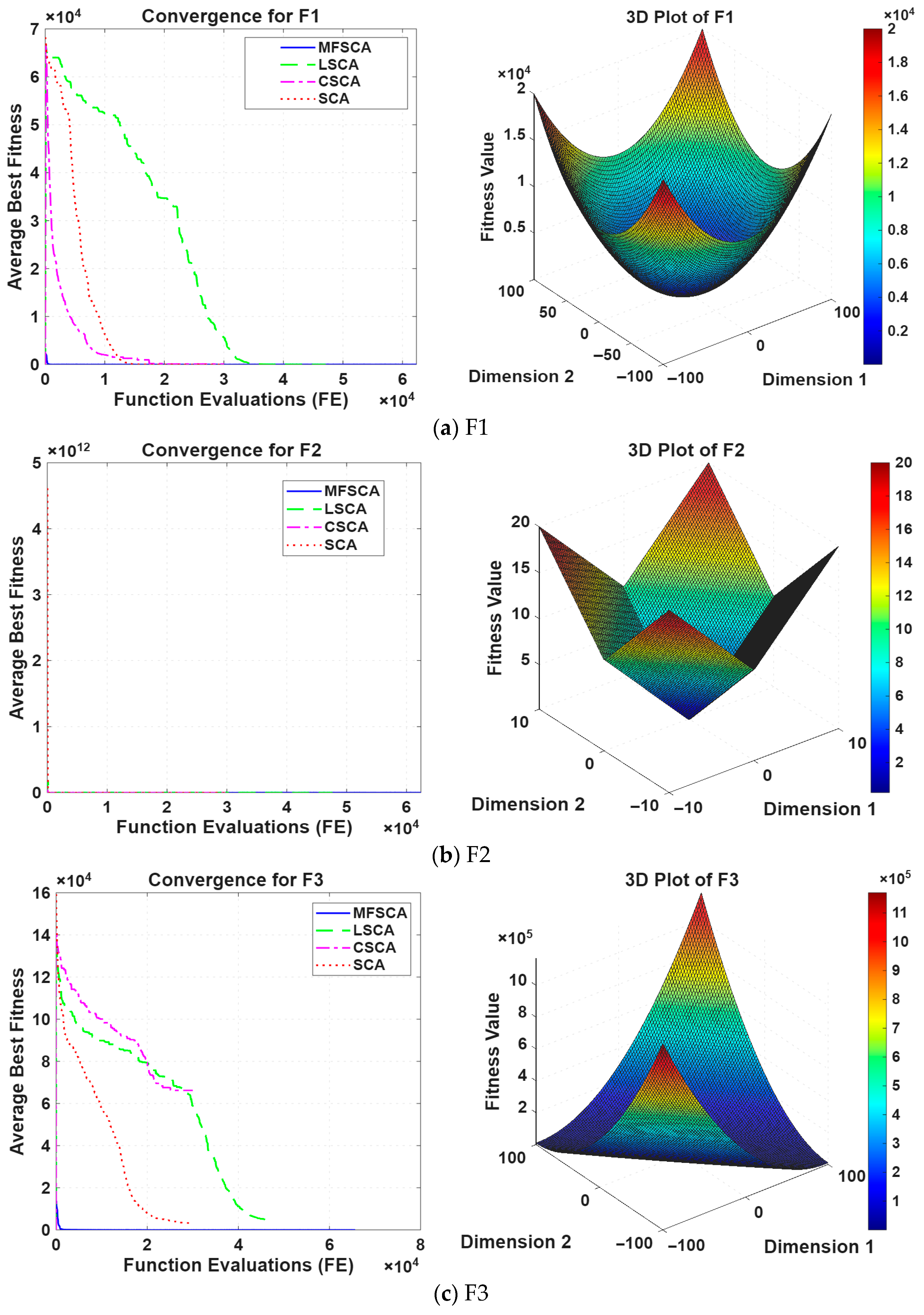
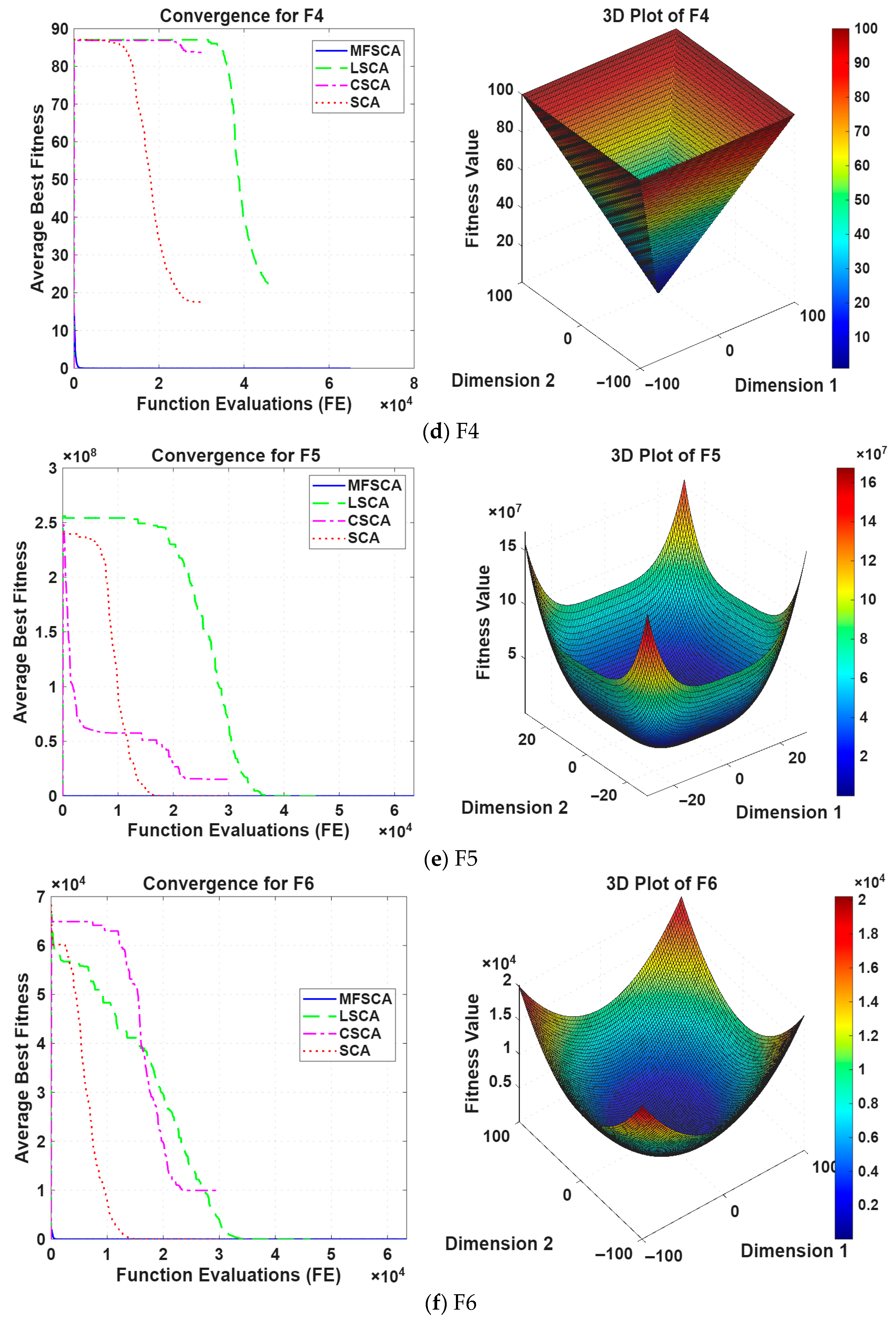
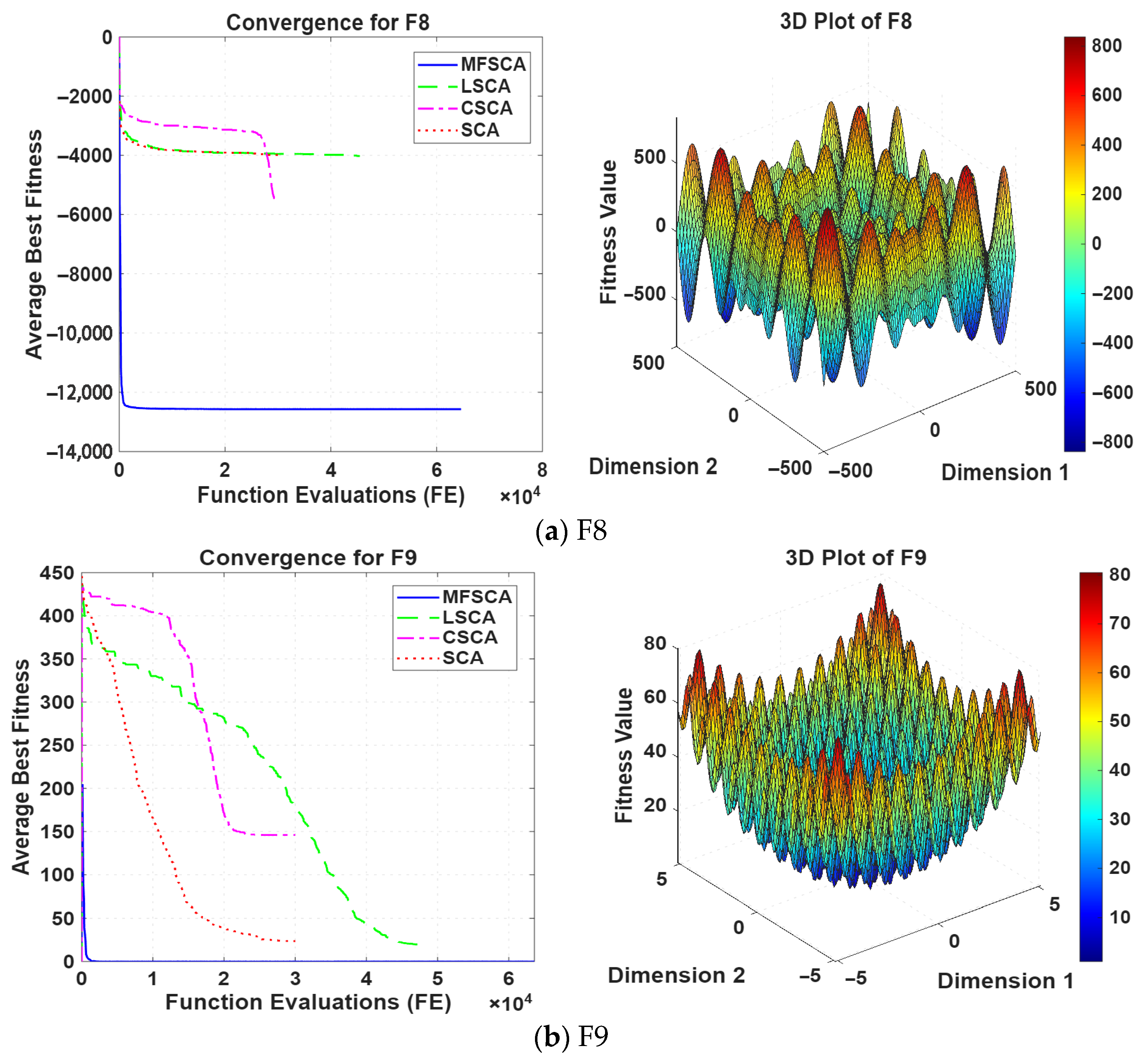
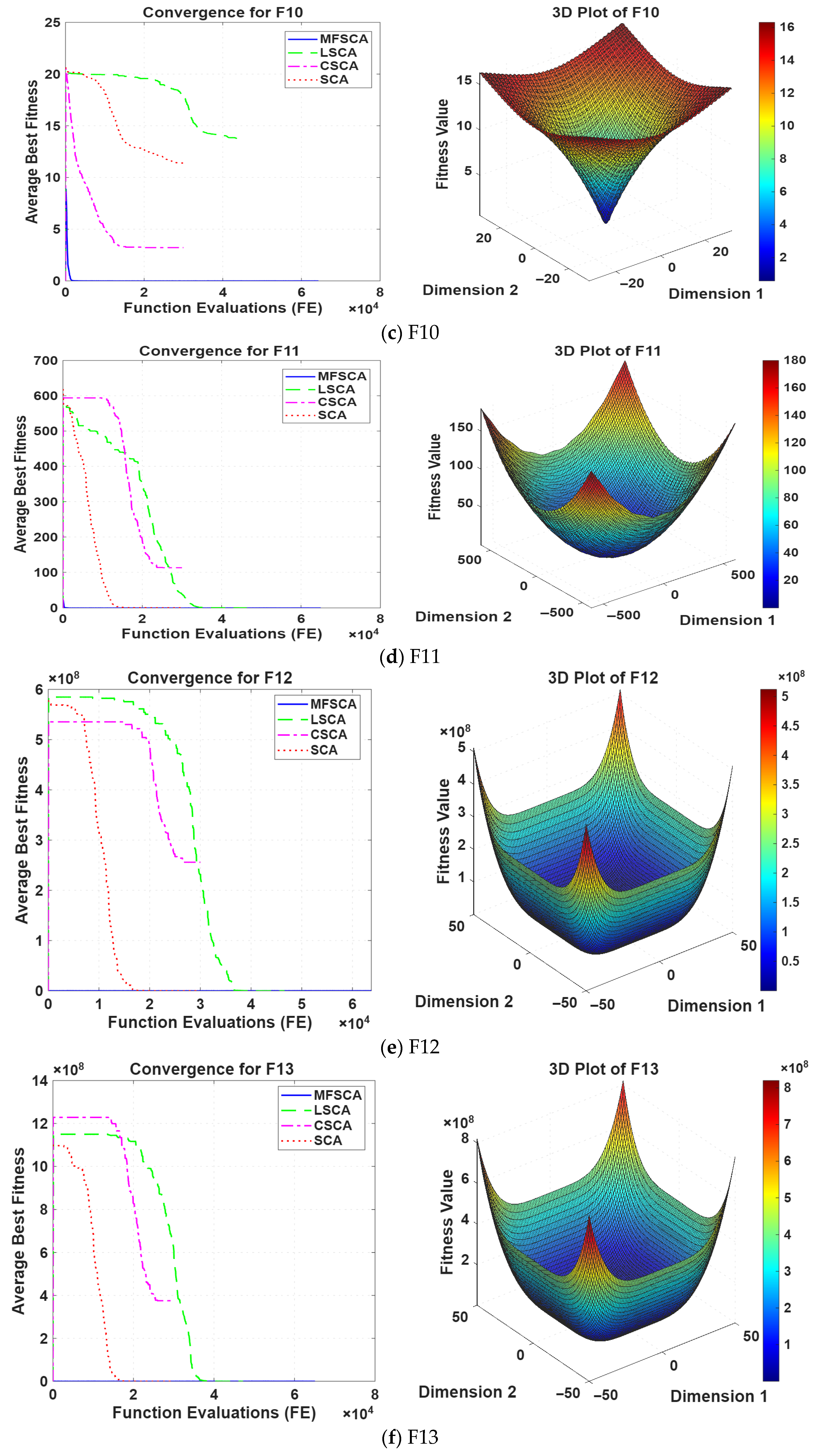
The figures in the next sections consist of the convergence plots and 3D plots. The vertical axis of the convergence curve represents the objective value or cost of the best solution found by the algorithm up to that point. Given that the plot is decreasing, the goal is minimization. This means that the lower the value, the better the solution the algorithm has found. It is worth noting that a value close to zero, or the global minimum value, indicates the algorithm has been able to successfully solve the problem. In addition, the function evaluation (FE) axis, which is the horizontal axis, represents the computational budget or the number of times the algorithm had to calculate the FE of the potential solution. It measures the computational cost of the algorithm.
On the other hand, the 3D plot has a color bar which represents the output of the objective function of any given function. It is the height of the surface, and the goal of the optimization is to find the lowest point on the surface, which is also known as the global minimum. The global minimum corresponds to the best solution. The red/yellow areas are high-cost, whereas the blue/green areas are low-cost.
Furthermore, Dimension 1 (X-axis) can be referred to as the value of the first variable in the optimization problem. Given that the problem has multiple variables to optimize, i.e., multi-dimensional, the plots are presented in two input dimensions for visualization. Dimension 2 (Y-axis), together with Dimension 1, defines a specific point on the input space where the algorithm searches for the minimum fitness value.

5.1.1. Evaluation of the Exploitation Capability

This section presents the performance results of the proposed MFSCA in comparison with the standard SCA and two other variants, CSCA and LSCA, using unimodal test functions that primarily assess the algorithms’ exploitative capabilities. Table 5 summarizes the experimental outcomes across four evaluation metrics: average fitness, standard deviation, best fitness, and worst fitness. The comparative analysis of the algorithms on the seven benchmark functions reveals distinct performance profiles. The MFSCA consistently demonstrated superior performance across all functions. This is evident in the unimodal Sphere function (Figure 2a), Schwefel 2.22 (Figure 2b), Schwefel 1.2 (Figure 2c), and Schwefel 2.21 (Figure 2d), which showed convergence to the global minimum with remarkable precision and stability. It can be inferred that MFSCA is highly effective at navigating landscapes with a single, clear minimum. In addition, its capability to handle more complex problems is confirmed on the Rosenbrock function (Figure 2e), which is known to be a very difficult test function due to its narrow valley. As seen in Figure 2e, the MFSCA maintained its performance by significantly outperforming the other algorithms.
Furthermore, on the discontinuous Step function and the noisy Quartic function (Figure 2f,g), MFSCA’s ability to handle abrupt changes and resist perturbations was evident, as its results were consistently better and more reliable than those of the other algorithms. In contrast, the performance of LSCA, CSCA, and SCA varied but was always inferior to MFSCA, indicating that the enhancements in MFSCA are crucial for achieving state-of-the-art results on this set of problems.

5.1.2. Evaluation of Exploration Capability

Functions F8–F13 specifically evaluate the exploration capabilities of the algorithms under multimodal landscapes (see Figure 3a–f). Since multimodal functions have many local optima, the algorithms’ performance on these functions demonstrates their ability to avoid local optima and navigate toward near-global optima. Consequently, the algorithm with the best results on these functions indicates a strong capacity for exploration and robustness in complex search spaces. Table 6 presents the results obtained in this category.
As shown in Table 6, the MFSCA maintained consistently superior performance across all multimodal functions (F8–F13), recording the lowest mean objective values. This is evident in the Schwefel 2.26 function (Figure 3a), where the mean, best, and worst values are the lowest, indicating that MFSCA converged precisely to the global minimum. The low standard deviation further demonstrates its stability and reliability. In the Rastrigin function (Figure 3b), MFSCA achieved the global minimum with zero deviation, confirming its ability to navigate highly oscillatory landscapes efficiently. Similarly, on the Ackley function (Figure 3c), MFSCA reached near-zero values for all statistical measures, outperforming LSCA, CSCA, and SCA, whose results were higher and more variable. The Griewank function (Figure 3d) further emphasizes MFSCA’s effectiveness, achieving perfect convergence with zero standard deviation, while the other algorithms struggled to reach similar accuracy and stability.
On the more challenging Penalised 1 (Figure 3e) and Penalised 2 (Figure 3f) functions, MFSCA maintained strong performance, producing consistently low mean and standard deviation values. This demonstrates its robustness in handling complex, high-dimensional, and irregular search spaces. In contrast, LSCA, CSCA, and SCA showed varied performance, with higher mean errors, larger deviations, and poorer convergence in most cases. These results clearly indicate that the modifications incorporated in MFSCA are crucial for achieving state-of-the-art performance on multimodal benchmark problems.

5.1.3. Fixed-Dimensional Multimodal Functions

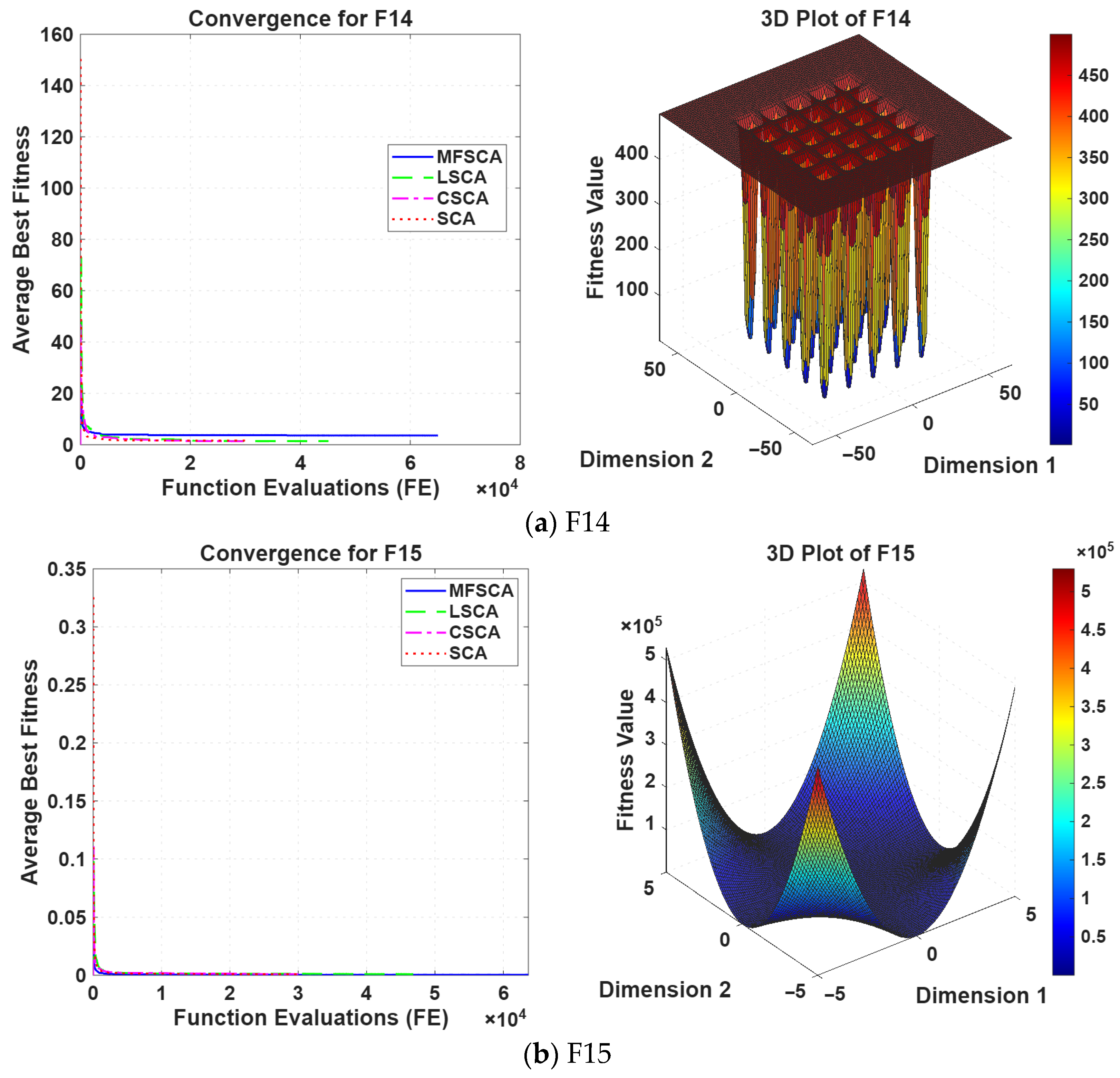
The performance of the proposed algorithm for fixed-dimension multimodal functions (F14–F23) in comparison with other algorithms is discussed in this section. The results obtained are shown in Table 7. Figure 4a–j show the convergence curve for each function. As revealed in Table 7, the LSCA delivered competitive performance by achieving the lowest values for F14 compared with other algorithms. However, for F14 (Figure 4a), while the mean value of MFSCA is somewhat higher, its best value matches the global optimum, indicating that it can still reach the optimal solution despite some variability.
In terms of Kowalik’s function (F15), the MFSCA maintained its best performance by achieving the lowest mean, standard deviation, best, and worst values. This confirms its stability and precision on smoother landscapes. The convergence curve is shown in Figure 4b.
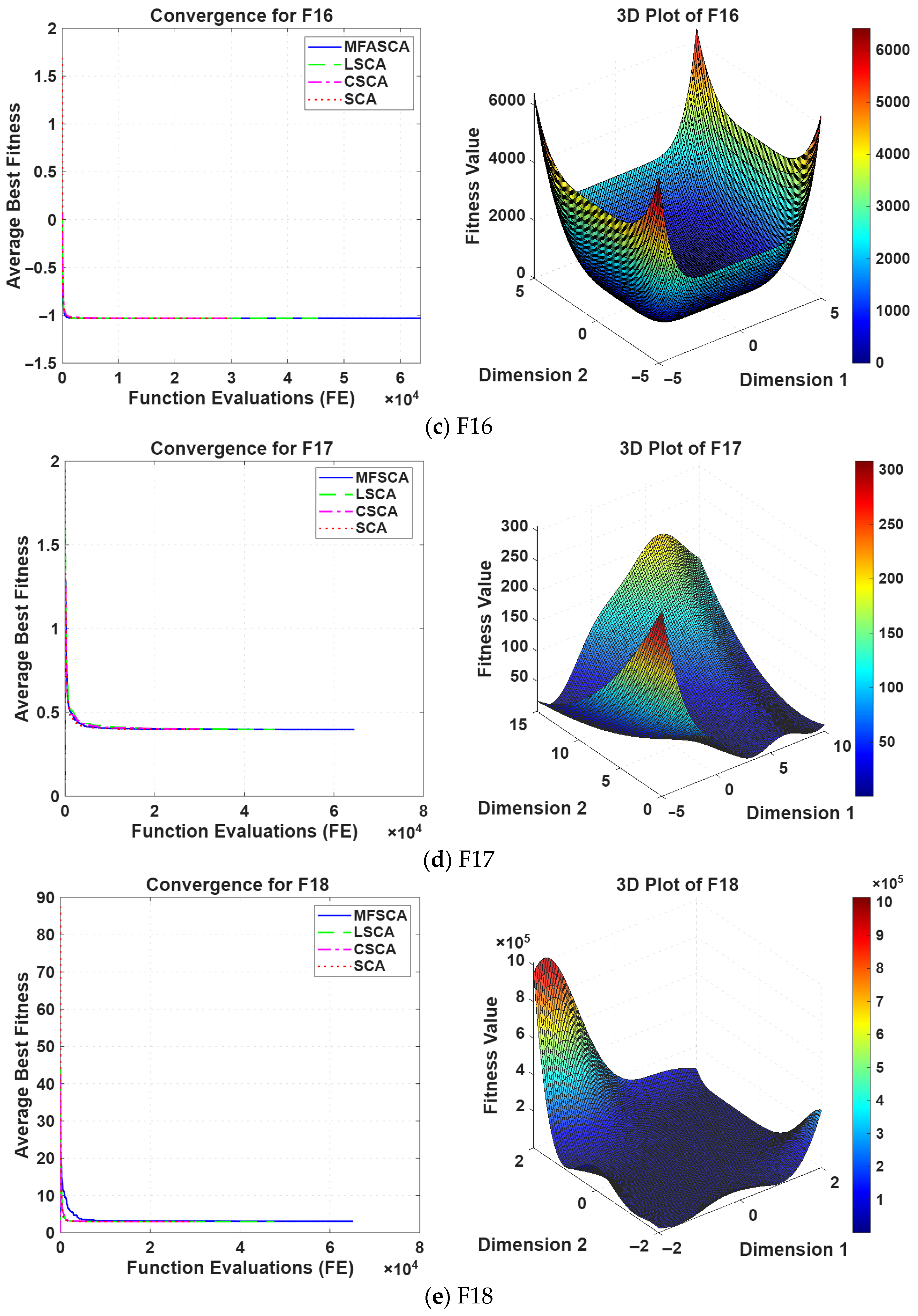
For the Six-Hump Camel function (F16), MFSCA shows near-identical results across all algorithms (Figure 4c), maintaining precise convergence and negligible deviation. For instance, MFSCA achieves the same mean, best, and worst values as other algorithms. Similarly, on F17 (Figure 4d), MFSCA exhibits high accuracy, low deviation, and best-case values comparable to or better than competing algorithms.
For F18, which corresponds to the Goldstein–Price function, LSCA delivered competitive performance, but MFSCA maintained tighter results (Figure 4e). For F19 (Figure 4f) and F20 (Figure 4g), MFSCA maintains robust performance with small standard deviations and best values that outperform the other algorithms, demonstrating its ability to handle moderately complex multimodal landscapes.
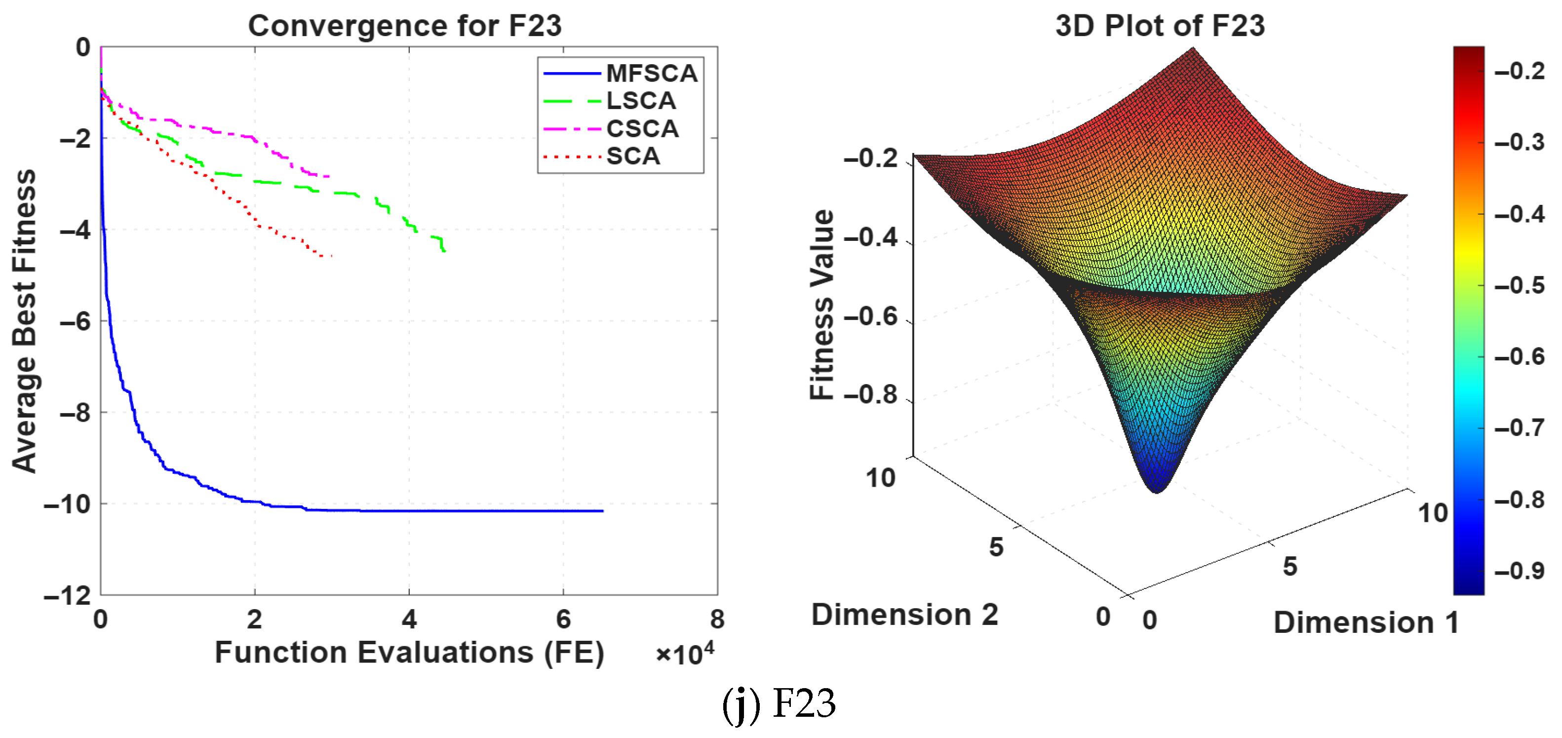
On the more challenging functions F21–F23 (Figure 4h–j), which feature highly irregular and deceptive landscapes, MFSCA significantly outperforms LSCA, CSCA, and SCA. Table 7 shows that its mean, best, and worst values consistently converge closer to the global optimum, indicating greater robustness. This highlights the effectiveness of MFSCA in solving complex optimization problems.
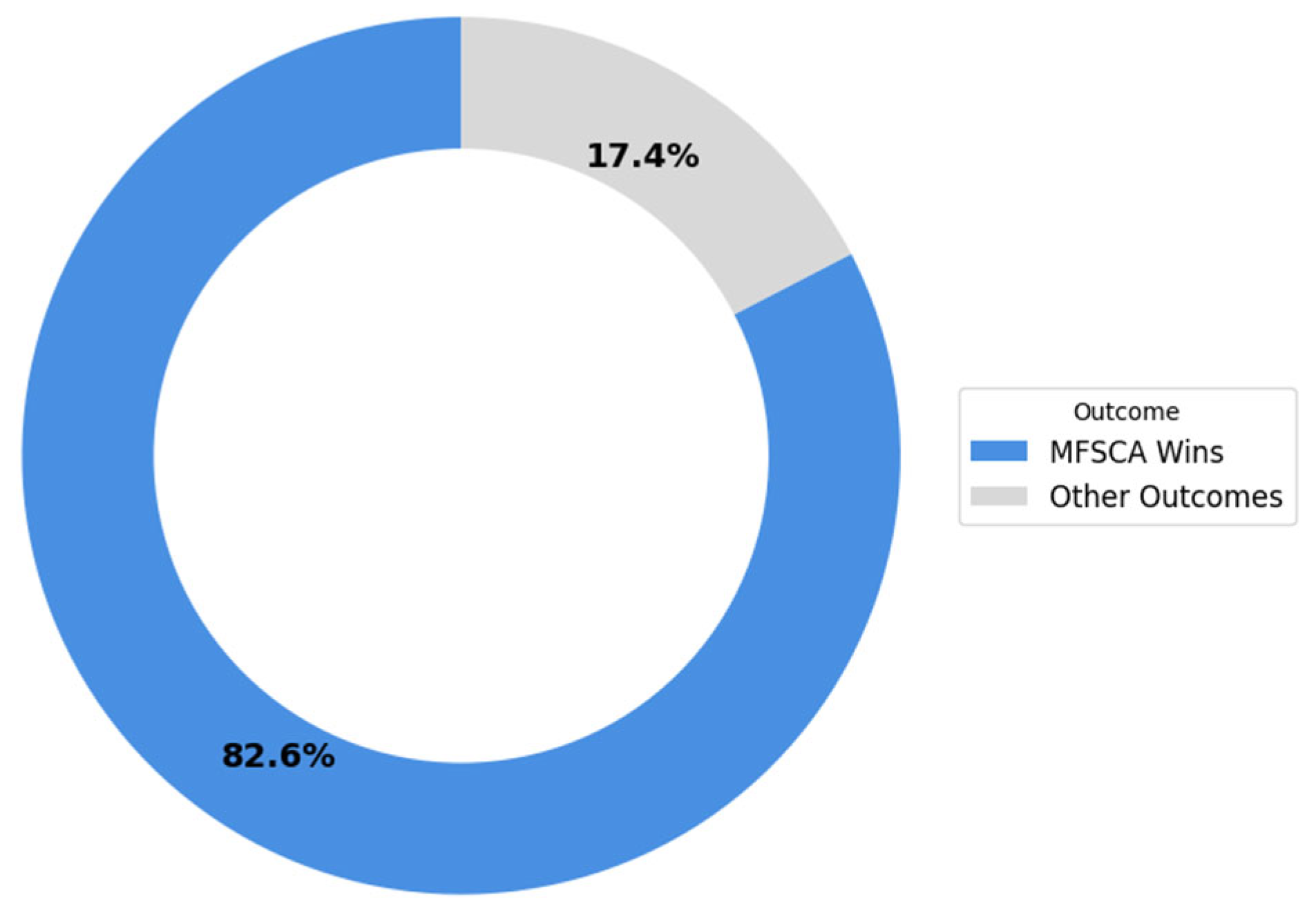
Figure 5 shows a chart that visually represents the proportion of functions where MFSCA was the top-performing algorithm. The chart is divided into two sections: the blue section, which occupies 82.6% of the chart, represents the 19 functions where MFSCA performed best, and the grey section, which occupies 17.4% of the chart, and represents the four functions where other algorithms performed better or tied with MFSCA. In short, the figure clearly shows that MFSCA was the overall best algorithm, winning on a large majority of the tested functions.

5.2. Statistical Analyses

Wilcoxon rank-sum is a non-parametric statistical method that uses common techniques to check if an algorithm is significantly better or worse than another algorithm based on their result distributions [82]. To determine whether the proposed MFSCA achieves notable enhancements over competing variants, this assessment compared the MFSCA results for each of the benchmark function with LSCA, CSCA, and standard SCA at a 5% significance threshold. If the p -value is less than 0.05, the null hypothesis is rejected, indicating a statistically significant difference at the chosen confidence level. Conversely, a p-value greater than 0.05 means the null hypothesis is accepted, implying little difference between the proposed method and the compared approaches. The outcomes of the Wilcoxon rank-sum test are presented in Table 8.
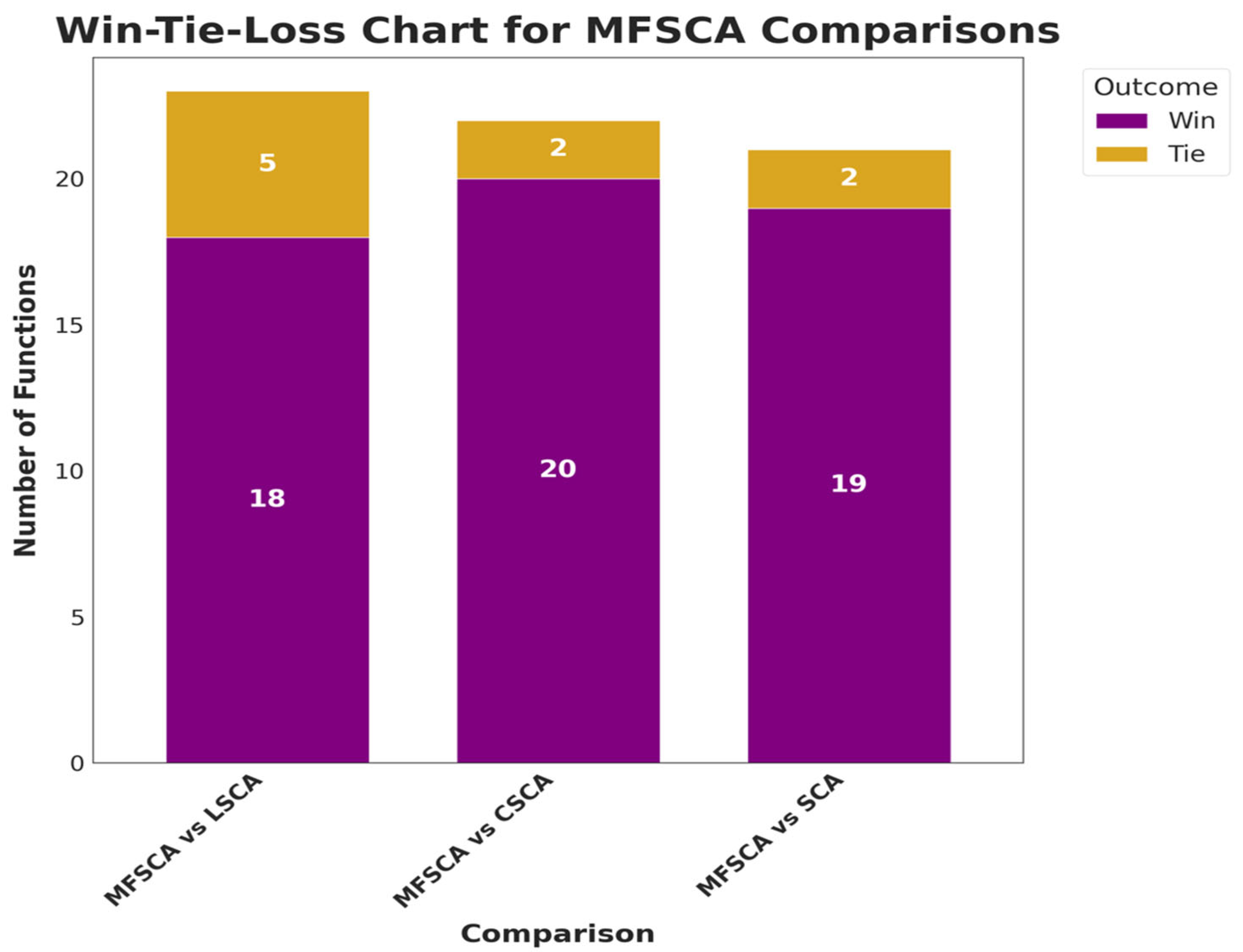
The results of the two-tailed Wilcoxon rank-sum test are provided in Table 8. Pairwise comparisons between the algorithms were conducted at a 0.05 significance level. In Table 8, the letter “ P ” indicates that MFSCA performs significantly while “ N ” denotes that there is no statistically significant difference between MFSCA and the algorithm it is compared with. The results of the Wilcoxon’s test which compared the performance of MFSCA against LSCA, CSCA, and SCA across 23 benchmark functions are presented in Table 8. As reported in the table, the proposed MFSCA performed better than other algorithms on the majority of functions. This points to the fact that the MFSCA is robust and effective across diverse optimization problems. However, a few functions such as the F14 and F16–F19 demonstrated a mixed or inferior performance. The overall results demonstrate that the MFSCA possesses strong competitive advantage and has great potential for general applicability in optimization tasks. Figure 6 summarizes the Win–Tie–Loss chart for the proposed MFSCA in comparison with other variants.
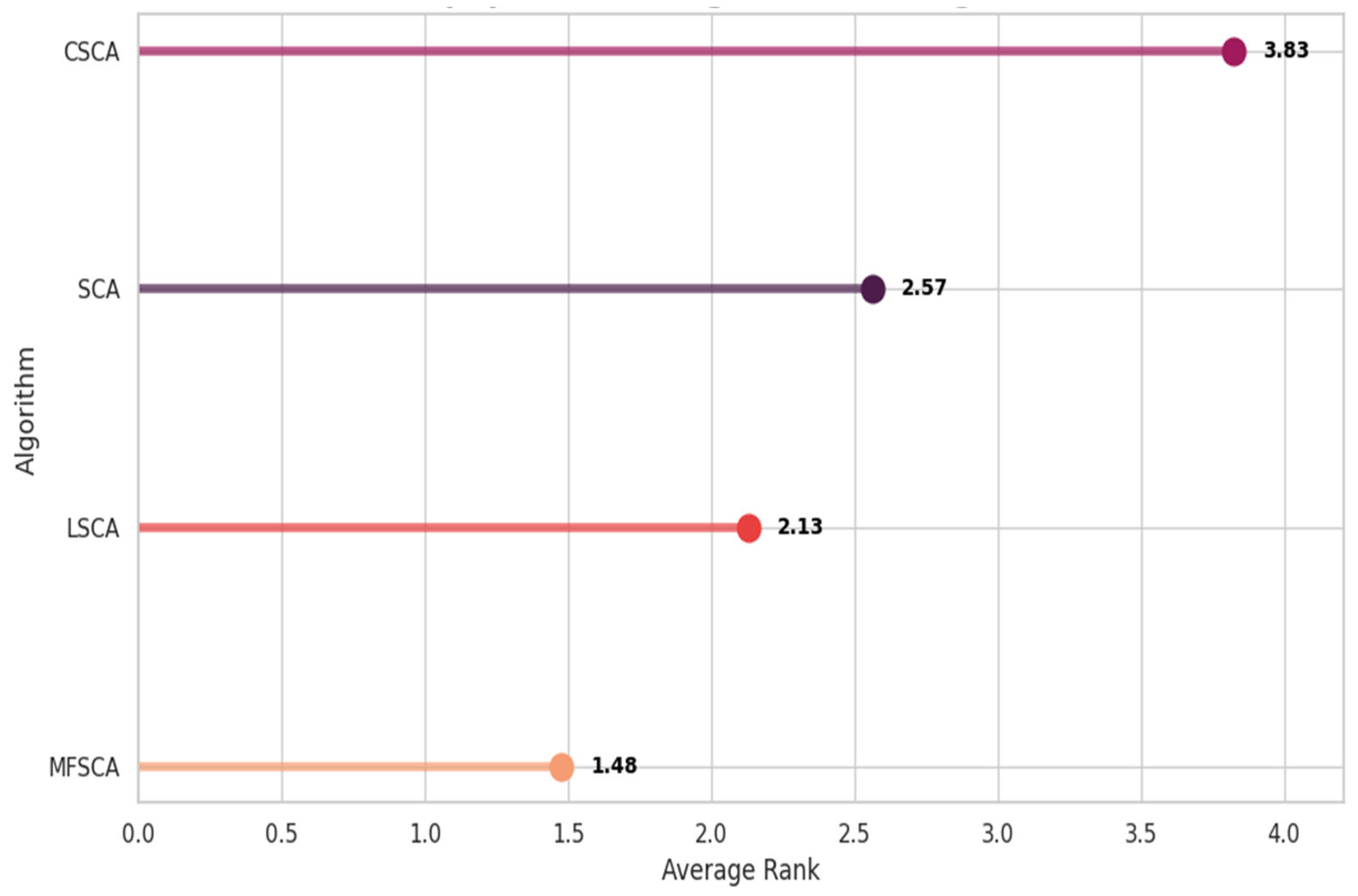
Furthermore, the Friedman rank-sum test was conducted to evaluate whether the proposed MFSCA algorithm provides a statistically significant improvement over the existing methods. In this test, algorithms are ranked according to their performance, with lower ranks representing better outcomes. As shown in Table 9, MFSCA attained the highest overall rank of 1.48 across all tested algorithms. Additionally, Figure 7 demonstrates that MFSCA consistently achieved performance equal to or better than the other algorithms on the majority of unimodal and multimodal benchmark functions. These results indicate that MFSCA surpasses the competing methods in effectiveness and reliability.

5.3. Algorithm Complexity

The proposed MFSCA is a multiple improvement on the standard SCA via the integration of different enhancement strategies as discussed in Section 3. Despite these enhancement strategies, the MFSCA’s theoretical time complexity remains linear with respect to the population size (N), problem dimensionality (D), and the maximum number of iterations (T), yielding O (N × D × T). This is comparable to other population-based metaheuristics that have been developed in the literature. Nevertheless, the practical implementation of MFSCA through additional operations increases the number of fitness evaluations per iteration. These additional enhancement strategies introduce a slightly sophisticated constant factor, thereby making the algorithm moderately more computationally involved than the basic SCA. However, this additional cost is offset by its significant gains in the proposed MFSCA convergence speed, exploration–exploitation balance, and accuracy in its solution. Therefore, the MFSCA can be considered computationally efficient and with better improvement. This makes it offer improved optimization performance without exponential growth in runtime.

6. Performance Evaluation of the Proposed MFSCA on Adaptive Neuro-Fuzzy Inference System

This section discusses the performance of the proposed MFSCA in optimizing the adaptive neuro-fuzzy inference system (ANFIS) in predicting electricity consumption of a student residence.

6.1. Study Area Description and Data Collection

Gauteng holds the distinction of being South Africa’s smallest province by land area, covering roughly 18,170 square kilometers (around 2% of the nation’s total). Geographically, Johannesburg is in Gauteng Province, near the tropics at latitude 26°120′ 08″ S, and longitude 28°02′ 37″ E, with an elevation of about 1767 m and a surface of 1645 k m 2 . Despite its size, Gauteng boasts the highest population density in South Africa. This densely populated region, which houses Johannesburg, the country’s largest city, is home to approximately 15.5 million people, accounting for a quarter of South Africa’s residents. Located near the tropics, Johannesburg experiences distinct seasons. Warm and humid summers with a maximum temperature of around 21 °C in January give way to cooler and drier winters with a minimum temperature of about 10 °C in July [83]. These seasonal shifts, particularly in temperature and humidity, significantly impact the lifestyles and energy consumption of Johannesburg’s inhabitants. Interestingly, summers tend to be longer than winters in this region.
This study investigates the energy consumption patterns of a student residence at a university in Johannesburg, South Africa. The study considers all four principal seasons in South Africa for 2017: autumn (1 March–May 31), winter (1 June–31 August), spring (1 September–30 November), and summer (1 December–28/29 February). Climatic variables, including wind speed, ambient temperature, and relative humidity, were sourced from nearby South African Weather Service (SAWS) stations to ensure alignment with the geographic location of the campus. The examined student residence consists of 17 rooms and includes a kitchen, a laundry area, and sanitary facilities comprising four toilets and bathrooms. Real-time power consumption data was collected using monitoring equipment installed on the building’s distribution panel. Energy consumption data for the student residents was obtained from the study by Masebinu et al. [84].

6.2. Adaptive Neuro-Fuzzy Inference System (ANFIS)

A neuro-fuzzy inference system (ANFIS) combines the adaptive learning properties of artificial neural networks with the self-learning ability of fuzzy inference systems to emulate expert decision-making [85,86]. In ANFIS, the Takagi–Sugeno fuzzy framework links the antecedent and consequent parts through a series of fuzzy rules. The system employs a hybrid learning strategy combining the least-squares method with back-propagation gradient descent: the least-squares technique estimates the linear parameters in the consequent layer, while gradient descent adjusts the non-linear parameters associated with the membership functions (MFs) in the premise layer. During the forward pass, the consequent parameters are optimized while keeping the premise parameters constant, and upon determining the best consequent values, the premise parameters are subsequently adjusted through back-propagation. Consequently, ANFIS parameters are classified into linear (consequent) and non-linear (premise) categories. For a fuzzy inference system with two inputs, x and y, and a single output F, the rule base specified in Equations (12) and (13) define the fuzzy logic rules that govern the system’s inferential process.
Rule   1 :   If   x is   I 1 and   y is   J 1 , F 1 = a 1 x + b 1 y + c 1
Rule   2 :   If   x is   I 2 and   y is   J 2 , F 2 = a 2 x + b 2 y + c 2
In this configuration, the MFs are designated as I 1 , I 2 , J 1 , and J 2 , with x and y serving as the system’s input variables and F 1 and F 2 representing the outputs. The nodes’ consequent parameters are expressed as a, b, and c. The ANFIS architecture has five distinct layers. The first layer handles the inputs. The second layer performs fuzzification. The third and fourth layers evaluate the rules. Finally, the fifth layer carries out defuzzification to get the output. Figure 8 shows the ANFIS structure.
The ANFIS architecture is composed of five layers: fuzzy, product, normalization, defuzzification, and output, as illustrated in Figure 8. Among these layers, the product, normalization, and defuzzification layers contain a fixed number of nodes, whereas the fuzzy and output layers are adaptive, allowing their nodes to adjust according to the model parameters. In the initial layer, each adaptive node represents a fuzzy membership function, and the aggregate output of the layer is computed using the following formula:
O j 1 = μ A j ( I 1 ) ,   j = 1,2
O j 1 = μ B j ( I 2 ) ,   j = 1,2
Additionally, the second layer consists of fixed nodes, where the firing strength of each rule is calculated according to Equation (16).
O j 2 = w j = μ A j I 1 × μ B j I 2 , j = 1,2
In the third layer, each node’s firing strength is scaled by normalization, which involves dividing the node’s individual firing strength by the sum of all nodes’ firing strengths, as expressed in Equation (17). Consequently, the normalized firing strengths in this layer are constrained within the interval from 0 to 1.
O j 3 = w i ¯ = w j w 1 + w 2 ,   j = 1,2
This layer is responsible for defuzzification, with each node being adaptive and utilizing learned functions. The nodes integrate the inputs with the normalized signals from the preceding layer to evaluate the contribution of the j th rule to the overall output, as expressed in Equation (18).
O j 4 = w j ¯ z j = w i ¯ p j I 1 + q j I 2 + r j
where p j , q j , and r j are the consequent parameters of the node j .
The fifth layer consists of fixed nodes that aggregate all incoming signals from the preceding layers using a summation function. This final integration produces the overall output of the ANFIS model, effectively consolidating the contributions of all rules processed in the earlier layers [87].
O j 5 = j w j ¯ z j = j w j z j j w j
Choosing the right clustering method plays a big role in how well the ANFIS model performs and how manageable it is. The kind of clustering used can strongly affect how accurately the model predicts results. Because of this, the following section investigates the clustering technique applied in this work.

Clustering Technique

Clustering is a technique used to categorize datasets into distinct groups, ensuring that each cluster represents a unique entity, thereby facilitating structured data organization. The proposed ANFIS utilizes fuzzy c-means (FCM) to classify data into fuzzy clusters, which are then employed to define MFs and develop the FIS structure. The FCM algorithm is an advanced clustering methodology that allows a single data point to have degrees of membership across multiple clusters rather than being assigned exclusively to one. This method operates by computing membership values for each data instance, where these values are proportionally assigned based on the relative proximity between the data point and the cluster centers. As an unsupervised learning approach, FCM is widely utilized in diverse scientific and engineering disciplines, including but not limited to image segmentation, medical diagnostics, astronomical data classification, chemical pattern recognition, and agricultural system modeling [88].
Within the framework of ANFIS, the determination of an appropriate membership function (MF) is a crucial and computationally intensive task, inherently formulated as a clustering-based optimization problem. The primary objective of the FCM approach in this context is to reduce the overall complexity of the fuzzy inference system by minimizing the number of fuzzy rules necessary for effective decision-making. The degree of association between data points and different clusters is established through an optimization process that minimizes the objective function. The mathematical formulation presented in Equation (20) systematically determines the optimal positioning of cluster centers by calculating the distance between each data point and the corresponding centroid for every fuzzy group n and vector x i , where i = 1, 2, …, n . This ensures an adaptive and computationally efficient clustering structure that enhances the accuracy and interpretability of the modeled system.
E = i = 1 N k = 0 n U i j m x i c j 2
The equation defines how each data point’s membership U i j m to a given cluster is calculated at each iteration, considering a weighting exponent m , the cluster centroid ( c j ), and the total number of clusters ( C ), ensuring membership values fall between 0 and 1.
  U i j = k = 1 C x i c j x i c j 2 m 1 1

6.3. Modified Sine Cosine Algorithm (MFSCA)-ANFIS

Figure 9 shows the optimization of the ANFIS using the proposed MFSCA for a predictive model. Figure 10 presents a two-stage hybrid system, named MFSCA-ANFIS, which combines the proposed algorithm with a fuzzy inference system. The hybrid model begins by implementing MFSCA, initializing a population of agents that represent potential solutions to a problem. The algorithm then iteratively calculates the objective function to evaluate the performance of each agent. The next steps are to identify the best solution and update the positions of all agents using a combination of chaotic maps and sine/cosine functions. This process is designed to find the optimal set of parameters for the subsequent model. The loop continues until a specific termination criterion is met, thereby ensuring that the algorithm has effectively explored the solution space to find a high-quality result.
As shown in Figure 9, the second stage begins with the creation of the ANFIS architecture after the optimization phase. The final population obtained from MFSCA is used to initialize the structure of ANFIS, including setting the number and type of MFs and defining the initial fuzzy rules. Next, a clustering technique is applied to the input data to establish the centers and spreads of these MFs. The main aim of this training is to iteratively minimize the output error until its own termination criteria are satisfied. The trained model is then validated by testing its performance on unseen data, and the accuracy is quantified by comparing the predicted outputs with the actual target values. This technical integration ensures that the ANFIS model is not only trained on data but also fundamentally structured with an optimized, problem-specific initial configuration. Consequently, MFSCA-ANFIS is applied to estimate the electricity consumption of a students’ residence.

Evaluating the Model Performance

Performance evaluation metrics also serve as essential benchmarking tools. This is a common practice to help identify the most reliable and accurate model for real-world deployment. Consequently, in this study, we utilize well-established performance indicators such as Mean Absolute Error (MAE), Coefficient of Variation of RMSE (CVRMSE), Mean Absolute Deviation (MAD), and Root Mean Square Error (RMSE) to evaluate the performance of the predictive model for forecasting electricity consumption. MAPE provides an intuitive measure of forecast accuracy in relative terms by quantifying the average percentage error between predicted and actual electricity consumption. MAE indicates overall accuracy by revealing the average absolute difference between predicted and actual line voltage values. RMSE highlights larger deviations, making it effective for detecting significant errors or outliers in the predictions. CVRMSE enables meaningful comparisons by providing a normalized measure of prediction error relative to the mean electricity consumption. Detailed descriptions of these metrics are provided in Table 10. Lower values are better for all metrics, and the best values are indicated in bold text. Key parameters used in configuring each model are summarized in Table 11.
In Table 10, y k denotes the observed values, y ^ k indicates the predicted values, and k corresponds to the sample index. The symbol Y ¯ represents the mean of the observed values.
The parameter settings of the algorithm used are presented in Table 11. The proposed hybrid MFSCA-ANFIS are compared with other hybrid algorithms consisting of classical and new generational metaheuristic algorithms such as the GA, Equilibrium Optimizer (EO) [89], Harris Hawks Optimization (HHO) algorithm [3], Biogeography-Based Optimization (BBO) [90], and Fox-Inspired Optimization Algorithm (FOA) [91] in order to assess comparative performance and accuracy. For a fair comparison, the same parameter values were used for parameters that are common to all algorithms. As shown in Table 3, the number of iterations and population size which are the parameters common to all the algorithms were utilized.

6.4. Results and Discussion of the MFSCA-ANFIS with Other Hybrid Models

This section discusses the performance of the different predictive models based on six metrics: RMSE, MAD, MAE, CVRMSE, U, and SD. These metrics reveal how each of the models are able to forecast electricity demand. This is crucial for optimizing energy supply, reducing wastage, and guaranteeing reliability in the student residences where consumption patterns can be highly variable. As reported in Table 12, it can be seen that the proposed MFSCA-ANFIS model yielded the lowest RMSE (1.9374) in the testing phase among all the evaluated models. Since RMSE measures the average magnitude of prediction errors, it can be inferred that the MFSCA-ANFIS produced the most accurate predictions among its counterparts.
Similarly, the lowest value of the MAD (1.5457) was delivered by the MFSCA-ANFIS. The MAD measures the average absolute difference between predicted and actual values. The lowest value produced by the MFSCA-ANFIS implies that its predictions are consistently close to actual consumption. Furthermore, the MFSCA-ANFIS surpassed its counterpart by demonstrating the lower MAE (1.5457), indicating the consistency and stability. In terms of the CVRMSE, the lowest value of 42.8463% was delivered by the MFSCA-ANFIS, showing that the model maintains consistent accuracy regardless of fluctuations in students’ electricity usage patterns, making it more dependable for managing demand variability in residences. The situation is different for the Theil’s U as both the CSCA and HHO-ANFIS (0.4209) demonstrated slightly better results; however, the MFSCA is very close (0.4224). The MFSCA-ANFIS retained its best performance with the lowest SD (1.9373), indicating less variation in prediction errors and having predictive errors tightly clustered around the mean.
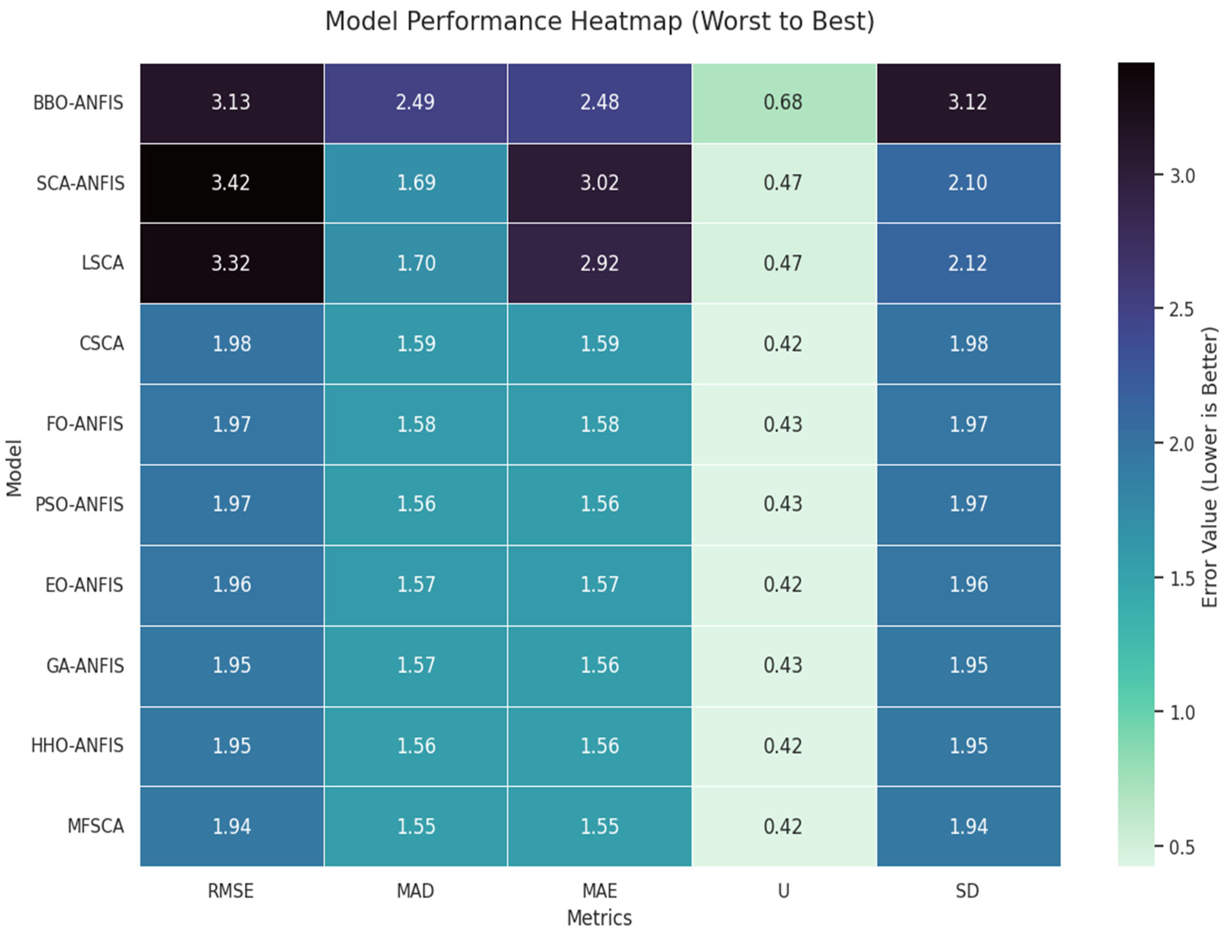
Figure 10 is the heatmap that visually compares the performance of ten different machine learning models across five key metrics. The models on the vertical axis are ranked from worst (BBO-ANFIS) at the top to best (MFSCA) at the bottom. The color of each cell corresponds to the numerical value within it. Darker colors represent higher error values (worse performance), while lighter colors represent lower error values (better performance). The heatmap provides a quick, concise way to see that models at the top (like BBO-ANFIS and SCA-ANFIS) perform poorly, while those at the bottom (like MFSCA and HHO-ANFIS) are the most effective. The performance of the MFSCA-ANFIS demonstrates a capability that can enable efficient scheduling of electricity supply for dormitories, avoiding shortages during peak times (e.g., evenings) or unnecessary energy wastage during low-demand periods. In addition, models with lower error variance (SD) help energy managers plan for predictable load fluctuations, important in student residences with varied daily activities. It is worth noting that reliable predictions can reduce the need for expensive emergency power procurement or penalties from overconsumption leading to cost efficiency.
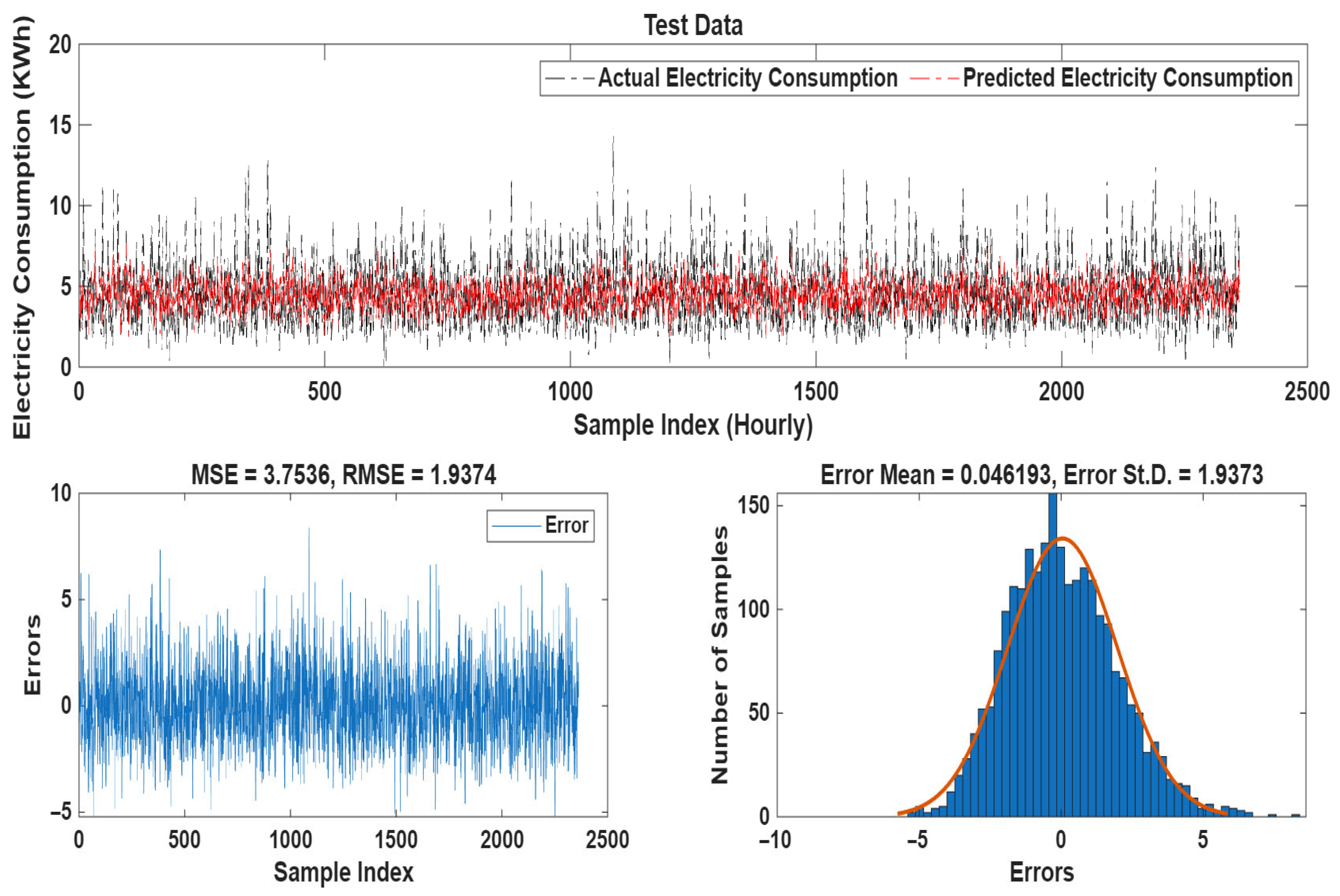
Figure 11 shows the graph of actual and predicted electricity consumption along with the error plots and histogram plots. This figure shows the performance of a time series forecasting model on a test dataset. It has three main plots that check how well the model predicts electricity consumption. The top plot is a time series graph. It compares the actual electricity consumption (dashed black line) with the predicted electricity consumption (dashed red line). The two lines are close to each other, which means the model gives good predictions. The second plot shows the prediction errors. These errors are the differences between the actual and predicted values. The errors move around zero, which is a good sign for the model. The third plot is a histogram of the errors. It has a bell shape that is centered near zero. An orange fitted curve shows this clearly. This means the errors are close to normal and not biased.
Figure 12 shows the performance pattern of the MFSCA-ANFIS model during testing and training phases. It can be observed from the figure that the percentage change from the Training to the Testing phase shows that the MFSCA-ANFIS model improved across all statistical metrics. In the figure, a negative percentage change indicates a reduction in error or uncertainty. Figure 12 reveals that all the metrics exhibited negative percentage across all the metrics pointing towards a positive outcome. The most significa2t improvement was seen in the Theil’s U metric (which showed a −2.20% decrease). Furthermore, the RMSE and SD values also saw notable reductions of −1.63% and −1.58%, respectively. The smallest improvements were in the MAD and MAE metrics, with decreases of −0.97% and −0.96%. Collectively, the model performed better during the Testing phase. This demonstrates a general trend of reduced error and uncertainty.

6.5. Limitations of the Study

This study focused on the development of the multi-faceted SCA and demonstrated its effectiveness through comparison with its variants. While the results are robust, effective, and reliable, future studies can explore additional enhancements and extend comparisons with a wider range of algorithms. Another important direction is the development of a multi-objective version of MFSCA to broaden its applications.

7. Conclusions

A multi-faceted SCA is proposed in this article. The efficacy of the proposed MFSCA is contingent on the integration of diverse enhancement strategies to improve the accuracy of search direction for optimization problems. The developed MFSCA benefits from the integration of diverse exploration–exploitation balancing strategies by first generating the initial population via a dynamic opposition mechanism to improve diversity and global search capability. Secondly, chaotic logistic maps are utilized to produce random coefficients to boost exploration, while an elite-learning strategy enables agents to learn from multiple top-performing solutions. In addition, adaptive parameters such as inertia weight, jumping rate, and local search strength are harnessed to guide the search process. Furthermore, Lévy flights and adaptive Gaussian local search with elitist selection are utilized to enhance exploration and exploitation, while ensuring sustained population diversity. The results obtained from the numerical experiments showed that the proposed MFSCA outshone its original SCA and other variants such as the Lévy-based SCA and chaotic-based SCA. In addition, a statistical study using Wilcoxon rank-sum and Friedman rank tests further demonstrated a significant improvement of the proposed MFSCA algorithm over other algorithms and having the best ranking in the comparative study. Furthermore, the proposed MFSCA was utilized to optimize the parameters of the fuzzy c-means adaptive neuro-fuzzy inference system for forecasting the electricity consumption for student residence occupancy prediction, using a university in Johannesburg residence in South Africa as a case study. The results obtained showed that the proposed MFSCA-ANFIS delivered the best performance by having the best RMSE (1.9374), MAD (1.5483), MAE (1.5457), CVRMSE (42.8463), and SD (1.9373), respectively.
In both scenarios, the results obtained demonstrated the efficacy of the developed algorithm in solving the optimization problem and for electricity prediction. The algorithm has the tendency to be able to contribute significantly to energy management where the projection of energy is critical.
Future studies may consider more enhancement by incorporating hybrid learning mechanisms into other functional components of the algorithm. In addition, the area of application can be extended to other areas of applications such as signal processing, image processing, and also considering the impact of clustering techniques in the adaptive neuro-fuzzy inference systems forecasting applications.

Author Contributions

Conceptualization: S.O.O., formal analysis: S.O.O., funding acquisition: S.O.O., U.B.A. and A.O.A., investigation: S.O.O., project administration: U.B.A., software: S.O.O., supervision: U.B.A., validation: S.O.O., U.B.A. and A.O.A., visualization: S.O.O., writing—original draft: S.O.O., writing—review and editing: U.B.A. and A.O.A. All authors have read and agreed to the published version of the manuscript.

Funding

This research received no external funding.

Data Availability Statement

The original contributions presented in this study are included in the article. Further inquiries can be directed to the corresponding author.

Acknowledgments

S. O. Oladipo acknowledges Tshwane University of Technology, South Africa, for the support provided for this study.

Conflicts of Interest

The authors declare no conflicts of interest.

Abbreviations

The following abbreviations are used in this manuscript:
SCASine Cosine Algorithm
DODynamic Opposition
MFSCAMulti-faceted
LSCALévy Sine Cosine Algorithm
CSCAChaotic Sine Cosine Algorithm
NINature Intelligence
MAMetaheuristic Algorithm
JOS Joint Opposition Selection
NFLNo Free Lunch Theorem
ANFISAdaptive Neuro-Fuzzy Inference System
SAWSSouth African Weather Service
MFMembership Function
FISFuzzy Inference System
FCMfuzzy c-means

References

  1. Bakır, H. Enhanced Artificial Hummingbird Algorithm for Global Optimization and Engineering Design Problems. Adv. Eng. Softw. 2024, 194, 103671. [Google Scholar] [CrossRef]
  2. Koop, L.; Maria, N.; Ramos, V.; Bonilla-Petriciolet, A.; Corazza, M.L.; Pedersen Voll, F.A. A Review of Stochastic Optimization Algorithms Applied in Food Engineering. Int. J. Chem. Eng. 2024, 2024, 3636305. [Google Scholar] [CrossRef]
  3. Heidari, A.A.; Mirjalili, S.; Faris, H.; Aljarah, I.; Mafarja, M.; Chen, H. Harris Hawks Optimization: Algorithm and Applications. Future Gener. Comput. Syst. 2019, 97, 849–872. [Google Scholar] [CrossRef]
  4. Zhang, R.; Wang, J.; Liu, C.; Su, K.; Ishibuchi, H.; Jin, Y. Synergistic Integration of Metaheuristics and Machine Learning: Latest Advances and Emerging Trends. Artif. Intell. Rev. 2025, 58, 268. [Google Scholar] [CrossRef]
  5. El-Shorbagy, M.A.; Bouaouda, A.; Abualigah, L.; Hashim, F.A. Stochastic Fractal Search: A Decade Comprehensive Review on Its Theory, Variants, and Applications. CMES Comput. Model. Eng. Sci. 2025, 142, 2339–2404. [Google Scholar] [CrossRef]
  6. Ahmed, A.M.; Rashid, T.A.; Hassan, B.A.; Majidpour, J.; Noori, K.A.; Rahman, C.M.; Abdalla, M.H.; Qader, S.M.; Tayfor, N.; Mohammed, N.B. Balancing Exploration and Exploitation Phases in Whale Optimization Algorithm: An Insightful and Empirical Analysis. In Handbook of Whale Optimization Algorithm: Variants, Hybrids, Improvements, and Applications; Academic Press: Cambridge, MA, USA, 2024; pp. 149–156. [Google Scholar] [CrossRef]
  7. Selvam, R.; Hiremath, P.; Cs, S.K.; Ramakrishna Bhat, R.; Tomar, V.; Bansal, M.; Singh, P. Metaheuristic Algorithms for Optimization: A Brief Review. Eng. Proc. 2023, 59, 238. [Google Scholar] [CrossRef]
  8. Oladipo, S.; Sun, Y. Assessment of a Consolidated Algorithm for Constrained Engineering Design Optimization and Unconstrained Function Optimization. In Proceedings of the 2nd International Conference on Robotics, Automation and Artificial Intelligence (RAAI), Singapore, 9–11 December 2022; pp. 188–192. [Google Scholar] [CrossRef]
  9. Cotta, C. Harnessing Memetic Algorithms: A Practical Guide. TOP 2025, 33, 327–356. [Google Scholar] [CrossRef]
  10. Tsai, C.W.; Chiang, M.C. Handbook of Metaheuristic Algorithms: From Fundamental Theories to Advanced Applications. In Handbook of Metaheuristic Algorithms: From Fundamental Theories to Advanced Applications; Elsevier: Amsterdam, The Netherlands, 2023; pp. 1–584. [Google Scholar] [CrossRef]
  11. Bhattacharyya, T.; Chatterjee, B.; Singh, P.K.; Yoon, J.H.; Geem, Z.W.; Sarkar, R. Mayfly in Harmony: A New Hybrid Meta-Heuristic Feature Selection Algorithm. IEEE Access 2020, 8, 195929–195945. [Google Scholar] [CrossRef]
  12. Michalewicz, Z.; Hinterding, R.; Michalewicz, M. Evolutionary Algorithms BT. In Fuzzy Evolutionary Computation; Pedrycz, W., Ed.; Springer: Boston, MA, USA, 1997; pp. 3–31. ISBN 978-1-4615-6135-4. [Google Scholar]
  13. Holland, J.H. Genetic Algorithms. Sci. Am. 1992, 267, 66–73. [Google Scholar] [CrossRef]
  14. Fogel, D.B.; Fogel, L.J. An Introduction to Evolutionary Programming. In Artificial Evolution; Lecture Notes in Computer Science (including subseries Lecture Notes in Artificial Intelligence and Lecture Notes in Bioinformatics); Springer: Berlin/Heidelberg, Germany, 1996; Volume 1063, pp. 21–33. [Google Scholar] [CrossRef]
  15. Storn, R.; Price, K. Differential Evolution-A Simple and Efficient Heuristic for Global Optimization over Continuous Spaces; Kluwer Academic Publishers: Dordrecht, The Netherlands, 1997; Volume 11. [Google Scholar]
  16. Alavi, M.; Henderson, J.C. An Evolutionary Strategy for Implementing a Decision Support System. Manag. Sci. 1981, 27, 1309–1323. [Google Scholar] [CrossRef]
  17. Dutta, T.; Bhattacharyya, S.; Dey, S.; Platos, J. Border Collie Optimization. IEEE Access 2020, 8, 109177–109197. [Google Scholar] [CrossRef]
  18. Eberhart, R.; Kennedy, J. A New Optimizer Using Particle Swarm Theory. In Proceedings of the Sixth International Symposium on Micro Machine and Human Science, Nagoya, Japan, 4–6 October 1995; IEEE: Piscataway, NJ, USA, 1995; pp. 39–43. [Google Scholar]
  19. Dorigo, M.; Gambardella, L.M. Ant Colony System: A Cooperative Learning Approach to the Traveling Salesman Problem. IEEE Trans. Evol. Comput. 1997, 1, 53–66. [Google Scholar] [CrossRef]
  20. Shah-Hosseini, H. The Intelligent Water Drops Algorithm: A Nature-Inspired Swarm-Based Optimization Algorithm. Int. J. Bio-Inspired Comput. 2009, 1, 71–79. [Google Scholar] [CrossRef]
  21. Mirjalili, S.; Mirjalili, S.M.; Lewis, A. Grey Wolf Optimizer. Adv. Eng. Softw. 2014, 69, 46–61. [Google Scholar] [CrossRef]
  22. He, S.; Wu, Q.H.; Saunders, J.R. Group Search Optimizer: An Optimization Algorithm Inspired by Animal Searching Behavior. IEEE Trans. Evol. Comput. 2009, 13, 973–990. [Google Scholar] [CrossRef]
  23. Passino, K.M. Biomimicry of Bacterial Foraging for Distributed Optimization and Control. IEEE Control Syst. 2002, 22, 52–67. [Google Scholar] [CrossRef]
  24. Duman, E.; Uysal, M.; Alkaya, A.F. Migrating Birds Optimization: A New Metaheuristic Approach and Its Performance on Quadratic Assignment Problem. Inf. Sci. 2012, 217, 65–77. [Google Scholar] [CrossRef]
  25. Rahmani, R.; Yusof, R. A New Simple, Fast and Efficient Algorithm for Global Optimization over Continuous Search-Space Problems: Radial Movement Optimization. Appl. Math. Comput. 2014, 248, 287–300. [Google Scholar] [CrossRef]
  26. Cuevas, E.; González, A.; Zaldívar, D.; Pérez-Cisneros, M. An Optimisation Algorithm Based on the Behaviour of Locust Swarms. Int. J. Bio-Inspired Comput. 2015, 7, 402–407. [Google Scholar] [CrossRef]
  27. Odili, J.B.; Kahar, M.N.M.; Anwar, S. African Buffalo Optimization: A Swarm-Intelligence Technique. Procedia Comput. Sci. 2015, 76, 443–448. [Google Scholar] [CrossRef]
  28. Harifi, S.; Khalilian, M.; Mohammadzadeh, J.; Ebrahimnejad, S. Emperor Penguins Colony: A New Metaheuristic Algorithm for Optimization. Evol. Intell. 2019, 12, 211–226. [Google Scholar] [CrossRef]
  29. Jain, M.; Singh, V.; Rani, A. A Novel Nature-Inspired Algorithm for Optimization: Squirrel Search Algorithm. Swarm Evol. Comput. 2019, 44, 148–175. [Google Scholar] [CrossRef]
  30. Chen, Z.; Francis, A.; Li, S.; Liao, B.; Xiao, D.; Ha, T.T.; Li, J.; Ding, L.; Cao, X. Egret Swarm Optimization Algorithm: An Evolutionary Computation Approach for Model Free Optimization. Biomimetics 2022, 7, 144. [Google Scholar] [CrossRef]
  31. Li, X.; Zhang, J.; Yin, M. Animal Migration Optimization: An Optimization Algorithm Inspired by Animal Migration Behavior. Neural Comput. Appl. 2014, 24, 1867–1877. [Google Scholar] [CrossRef]
  32. Dehghani, M.; Trojovská, E.; Trojovský, P. A New Human-Based Metaheuristic Algorithm for Solving Optimization Problems on the Base of Simulation of Driving Training Process. Sci. Rep. 2022, 12, 9924. [Google Scholar] [CrossRef]
  33. Matoušová, I.; Trojovský, P.; Dehghani, M.; Trojovská, E.; Kostra, J. Mother Optimization Algorithm: A New Human-Based Metaheuristic Approach for Solving Engineering Optimization. Sci. Rep. 2023, 13, 10312. [Google Scholar] [CrossRef]
  34. Trojovská, E.; Dehghani, M. A New Human-Based Metahurestic Optimization Method Based on Mimicking Cooking Training. Sci. Rep. 2022, 12, 14861. [Google Scholar] [CrossRef]
  35. Rao, R.V.; Savsani, V.J.; Vakharia, D.P. Teaching-Learning-Based Optimization: A Novel Method for Constrained Mechanical Design Optimization Problems. CAD Comput. Aided Des. 2011, 43, 303–315. [Google Scholar] [CrossRef]
  36. Hubalovska, M.; Major, S. A New Human-Based Metaheuristic Algorithm for Solving Optimization Problems Based on Technical and Vocational Education and Training. Biomimetics 2023, 8, 508. [Google Scholar] [CrossRef] [PubMed]
  37. Elsisi, M. Future Search Algorithm for Optimization. Evol. Intell. 2019, 12, 21–31. [Google Scholar] [CrossRef]
  38. Askari, Q.; Younas, I.; Saeed, M. Political Optimizer: A Novel Socio-Inspired Meta-Heuristic for Global Optimization. Knowl. Based Syst. 2020, 195, 105709. [Google Scholar] [CrossRef]
  39. Kumar, M.; Kulkarni, A.J.; Satapathy, S.C. Socio Evolution & Learning Optimization Algorithm: A Socio-Inspired Optimization Methodology. Future Gener. Comput. Syst. 2018, 81, 252–272. [Google Scholar] [CrossRef]
  40. Askari, Q.; Saeed, M.; Younas, I. Heap-Based Optimizer Inspired by Corporate Rank Hierarchy for Global Optimization. Expert. Syst. Appl. 2020, 161, 113702. [Google Scholar] [CrossRef]
  41. Lian, J.; Hui, G. Human Evolutionary Optimization Algorithm. Expert. Syst. Appl. 2024, 241, 122638. [Google Scholar] [CrossRef]
  42. Zhu, D.; Wang, S.; Zhou, C.; Yan, S.; Xue, J. Human Memory Optimization Algorithm: A Memory-Inspired Optimizer for Global Optimization Problems. Expert. Syst. Appl. 2024, 237, 121597. [Google Scholar] [CrossRef]
  43. Givi, H.; Dehghani, M.; Hubalovsky, S. Red Panda Optimization Algorithm: An Effective Bio-Inspired Metaheuristic Algorithm for Solving Engineering Optimization Problems. IEEE Access 2023, 11, 57203–57227. [Google Scholar] [CrossRef]
  44. Ni, L.; Ping, Y.; Yao, N.; Jiao, J.; Wang, G. Literature Research Optimizer: A New Human-Based Metaheuristic Algorithm for Optimization Problems. Arab. J. Sci. Eng. 2024, 49, 12817–12865. [Google Scholar] [CrossRef]
  45. Li, C.; Zhou, J. Parameters Identification of Hydraulic Turbine Governing System Using Improved Gravitational Search Algorithm. Energy Convers. Manag. 2011, 52, 374–381. [Google Scholar] [CrossRef]
  46. Lam, A.Y.S.; Li, V.O.K. Chemical-Reaction-Inspired Metaheuristic for Optimization. IEEE Trans. Evol. Comput. 2010, 14, 381–399. [Google Scholar] [CrossRef]
  47. Hatamlou, A. Black Hole: A New Heuristic Optimization Approach for Data Clustering. Inf. Sci. 2013, 222, 175–184. [Google Scholar] [CrossRef]
  48. Doğan, B.; Ölmez, T. A New Metaheuristic for Numerical Function Optimization: Vortex Search Algorithm. Inf. Sci. 2015, 293, 125–145. [Google Scholar] [CrossRef]
  49. Zheng, Y.J. Water Wave Optimization: A New Nature-Inspired Metaheuristic. Comput. Oper. Res. 2015, 55, 1–11. [Google Scholar] [CrossRef]
  50. Shareef, H.; Ibrahim, A.A.; Mutlag, A.H. Lightning Search Algorithm. Appl. Soft Comput. 2015, 36, 315–333. [Google Scholar] [CrossRef]
  51. Abedinpourshotorban, H.; Mariyam Shamsuddin, S.; Beheshti, Z.; Jawawi, D.N.A. Electromagnetic Field Optimization: A Physics-Inspired Metaheuristic Optimization Algorithm. Swarm Evol. Comput. 2016, 26, 8–22. [Google Scholar] [CrossRef]
  52. Mirjalili, S. SCA: A Sine Cosine Algorithm for Solving Optimization Problems. Knowl. Based Syst. 2016, 96, 120–133. [Google Scholar] [CrossRef]
  53. Azizi, M.; Aickelin, U.; Khorshidi, H.A.; Baghalzadeh Shishehgarkhaneh, M. Energy Valley Optimizer: A Novel Metaheuristic Algorithm for Global and Engineering Optimization. Sci. Rep. 2023, 13, 226. [Google Scholar] [CrossRef] [PubMed]
  54. Kaveh, A.; Dadras, A. A Novel Meta-Heuristic Optimization Algorithm: Thermal Exchange Optimization. Adv. Eng. Softw. 2017, 110, 69–84. [Google Scholar] [CrossRef]
  55. Qais, M.H.; Hasanien, H.M.; Alghuwainem, S.; Loo, K.H. Propagation Search Algorithm: A Physics-Based Optimizer for Engineering Applications. Mathematics 2023, 11, 4224. [Google Scholar] [CrossRef]
  56. Wei, Z.; Huang, C.; Wang, X.; Han, T.; Li, Y. Nuclear Reaction Optimization: A Novel and Powerful Physics-Based Algorithm for Global Optimization. IEEE Access 2019, 7, 66084–66109. [Google Scholar] [CrossRef]
  57. Abdel-Basset, M.; Mohamed, R.; Azeem, S.A.A.; Jameel, M.; Abouhawwash, M. Kepler Optimization Algorithm: A New Metaheuristic Algorithm Inspired by Kepler’s Laws of Planetary Motion. Knowl. Based Syst. 2023, 268, 110454. [Google Scholar] [CrossRef]
  58. Kundu, R.; Chattopadhyay, S.; Nag, S.; Navarro, M.A.; Oliva, D. Prism Refraction Search: A Novel Physics-Based Metaheuristic Algorithm. J. Supercomput. 2024, 80, 10746–10795. [Google Scholar] [CrossRef]
  59. Kaveh, A.; Talatahari, S. A Novel Heuristic Optimization Method: Charged System Search. Acta Mech. 2010, 213, 267–289. [Google Scholar] [CrossRef]
  60. Wang, M.; Lu, G. A Modified Sine Cosine Algorithm for Solving Optimization Problems. IEEE Access 2021, 9, 27434–27450. [Google Scholar] [CrossRef]
  61. Shang, C.; Zhou, T.; Liu, S. Optimization of Complex Engineering Problems Using Modified Sine Cosine Algorithm. Sci. Rep. 2022, 12, 1–25. [Google Scholar] [CrossRef] [PubMed]
  62. Pham, V.H.S.; Nguyen Dang, N.T.; Nguyen, V.N. Enhancing Engineering Optimization Using Hybrid Sine Cosine Algorithm with Roulette Wheel Selection and Opposition-Based Learning. Sci. Rep. 2024, 14, 694. [Google Scholar] [CrossRef]
  63. Liu, J.; Bi, C.; Chen, H.; Heidari, A.A.; Chen, H. Triangular-Based Sine Cosine Algorithm for Global Search and Feature Selection. Sci. Rep. 2025, 15, 12992. [Google Scholar] [CrossRef]
  64. Cheng, J.; Lin, Q.; Xiong, Y. Engineering Optimization Sine Cosine Algorithm with Peer Learning for Global Numerical Optimization Sine Cosine Algorithm with Peer Learning for Global Numerical Optimization. Eng. Optim. 2024, 57, 963–980. [Google Scholar] [CrossRef]
  65. Wolpert, D.H.; Macready, W.G. No Free Lunch Theorems for Optimization. IEEE Trans. Evol. Comput. 1997, 1, 67–82. [Google Scholar] [CrossRef]
  66. Dudek, G.; Piotrowski, P.; Baczyński, D. Forecasting in Modern Power Systems: Challenges, Techniques, and Emerging Trends. Energies 2025, 18, 3589. [Google Scholar] [CrossRef]
  67. Li, P.; Hu, Z.; Shen, Y.; Cheng, X.; Alhazmi, M. Short-Term Electricity Load Forecasting Based on Large Language Models and Weighted External Factor Optimization. Sustain. Energy Technol. Assess. 2025, 82, 104449. [Google Scholar] [CrossRef]
  68. Pachauri, R.K.; Pandey, J.K.; Sharma, A.; Nautiyal, O.P.; Ram, M. Applied Soft Computing and Embedded System Applications in Solar Energy; CRC Press: Boca Raton, FL, USA, 2021. [Google Scholar]
  69. Oladipo, S.; Sun, Y.; Wang, Z. Pelican Optimization Algorithm-Based ANFIS for Bolstered Electricity Usage Prediction. In Proceedings of the 8th International Conference on Computer Science and Artificial Intelligence, Beijing, China, 8–9 December 2024; pp. 537–543. [Google Scholar] [CrossRef]
  70. Du, P.; Ye, Y.; Wu, H.; Wang, J. Study on Deterministic and Interval Forecasting of Electricity Load Based on Multi-Objective Whale Optimization Algorithm and Transformer Model. Expert Syst. Appl. 2025, 268, 126361. [Google Scholar] [CrossRef]
  71. Wei, H.L.; Abhishek, S. 7 Overview of Swarm Intelligence Techniques for Harvesting Solar Energy. In Recent Advances in Energy Harvesting Technologies; River Publishers: Gistrup, Denmark, 2023; pp. 161–176. [Google Scholar]
  72. Oladipo, S.; Sun, Y.; Adegoke, S.A. Hybrid Neuro-Fuzzy Modeling for Electricity Consumption Prediction in a Middle-Income Household in Gauteng, South Africa: Utilizing Fuzzy C-Means Method. In Neural Computing for Advanced Applications; Springer: Berlin/Heidelberg, Germany, 2025; pp. 59–73. [Google Scholar] [CrossRef]
  73. Al-Qaness, M.A.A.; Elaziz, M.A.; Ewees, A.A. Oil Consumption Forecasting Using Optimized Adaptive Neuro-Fuzzy Inference System Based on Sine Cosine Algorithm. IEEE Access 2018, 6, 68394–68402. [Google Scholar] [CrossRef]
  74. Yılmaz, S.; Yıldırım, A.A.; Feyzullahoğlu, E. Erosion Rate of AA6082-T6 Aluminum Alloy Subjected to Erosive Wear Determined by the Meta-Heuristic (SCA) Based ANFIS Method. Mater./Mater. Test. 2024, 66, 248–261. [Google Scholar] [CrossRef]
  75. Ehteram, M.; Yenn Teo, F.; Najah Ahmed, A.; Dashti Latif, S.; Feng Huang, Y.; Abozweita, O.; Al-Ansari, N.; El-Shafie, A. Performance Improvement for Infiltration Rate Prediction Using Hybridized Adaptive Neuro-Fuzzy Inferences System (ANFIS) with Optimization Algorithms. Ain Shams Eng. J. 2021, 12, 1665–1676. [Google Scholar] [CrossRef]
  76. Bansal, J.C.; Bajpai, P.; Rawat, A.; Nagar, A.K. Sine Cosine Algorithm. In Sine Cosine Algorithm for Optimization; SpringerBriefs in Applied Sciences and Technology; Springer: Berlin/Heidelberg, Germany, 2023; pp. 15–33. [Google Scholar] [CrossRef]
  77. Rahnamayan, S.; Tizhoosh, H.R.; Salama, M.M.A. Quasi-Oppositional Differential Evolution. In Proceedings of the 2007 IEEE Congress on Evolutionary Computation, Singapore, 25–28 September 2007; pp. 2229–2236. [Google Scholar]
  78. Ergezer, M.; Simon, D.; Du, D. Oppositional Biogeography-Based Optimization. In Proceedings of the 2009 IEEE International Conference on Systems, Man and Cybernetics, San Antonio, TX, USA, 11–14 October 2009; pp. 1009–1014. [Google Scholar]
  79. Xu, Y.; Yang, Z.; Li, X.; Kang, H.; Yang, X. Dynamic Opposite Learning Enhanced Teaching–Learning-Based Optimization. Knowl. Based Syst. 2020, 188, 104966. [Google Scholar] [CrossRef]
  80. Shi, Y.; Eberhart, R. Modified Particle Swarm Optimizer. In Proceedings of the IEEE Conference on Evolutionary Computation, ICEC, Nayoya, Japan, 20–22 May 1996; IEEE: Anchorage, AK, USA, 1998; pp. 69–73. [Google Scholar]
  81. Feng, H.; Ni, H.; Zhao, R.; Zhu, X. An Enhanced Grasshopper Optimization Algorithm to the Bin Packing Problem. J. Control Sci. Eng. 2020, 2020, 3894987. [Google Scholar] [CrossRef]
  82. Dao, P.B. On Wilcoxon Rank Sum Test for Condition Monitoring and Fault Detection of Wind Turbines. Appl. Energy 2022, 318, 119209. [Google Scholar] [CrossRef]
  83. Adeleke, O.; Akinlabi, S.; Jen, T.C.; Dunmade, I. A Machine Learning Approach for Investigating the Impact of Seasonal Variation on Physical Composition of Municipal Solid Waste. J. Reliab. Intell. Environ. 2022, 9, 99–118. [Google Scholar] [CrossRef]
  84. Masebinu, S.O.; Holm-Nielsen, J.B.; Mbohwa, C.; Padmanaban, S.; Nwulu, N. Electricity Consumption Data of a Student Residence in Southern Africa. Data Brief 2020, 32, 106150. [Google Scholar] [CrossRef]
  85. Oladipo, S.; Sun, Y.; Adeleke, O. An Improved Particle Swarm Optimization and Adaptive Neuro-Fuzzy Inference System for Predicting the Energy Consumption of University Residence. Int. Trans. Electr. Energy Syst. 2023, 2023, 8508800. [Google Scholar] [CrossRef]
  86. Rahman, M.S.; Ali, M.H. Adaptive Neuro Fuzzy Inference System (ANFIS)-Based Control for Solving the Misalignment Problem in Vehicle-to-Vehicle Dynamic Wireless Charging Systems. Electronics 2025, 14, 507. [Google Scholar] [CrossRef]
  87. Petković, D.; Ćojbašić, Ž.; Nikolić, V.; Shamshirband, S.; Mat Kiah, M.L.; Anuar, N.B.; Abdul Wahab, A.W. Adaptive Neuro-Fuzzy Maximal Power Extraction of Wind Turbine with Continuously Variable Transmission. Energy 2014, 64, 868–874. [Google Scholar] [CrossRef]
  88. Jayaprabha, M.; Felcy, P. A Review of Clustering, Its Types and Techniques. Int. J. Innov. Sci. Res. Technol. 2018, 3, 127–130. [Google Scholar]
  89. Faramarzi, A.; Heidarinejad, M.; Stephens, B.; Mirjalili, S. Equilibrium Optimizer: A Novel Optimization Algorithm. Knowl. Based Syst. 2020, 191, 105190. [Google Scholar] [CrossRef]
  90. Simon, D. Biogeography-Based Optimization. IEEE Trans. Evol. Comput. 2008, 12, 702–713. [Google Scholar] [CrossRef]
  91. Mohammed, H.; Rashid, T. FOX: A FOX-Inspired Optimization Algorithm. Appl. Intell. 2023, 53, 1030–1050. [Google Scholar] [CrossRef]
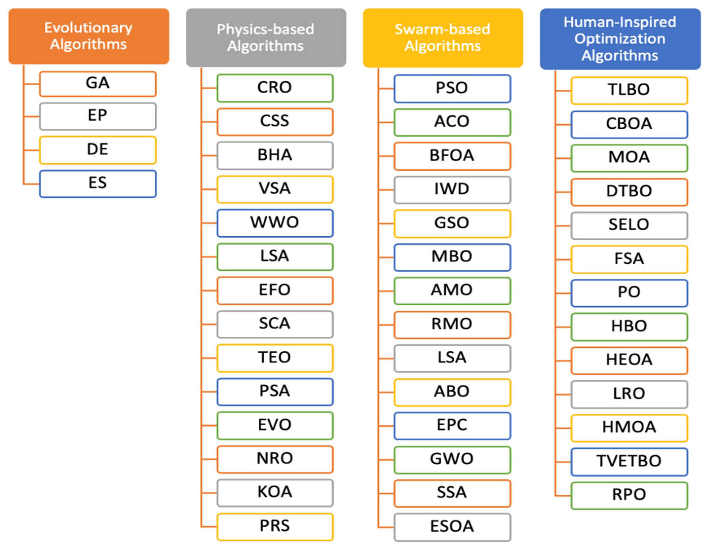
Figure 1. Classification of metaheuristic algorithms.
Computers 14 00444 g001
Figure 2. Convergence curves for unimodal test functions (F1–F7) and their respective 3D function plots.
Computers 14 00444 g002aComputers 14 00444 g002bComputers 14 00444 g002c
Figure 3. Convergence curves for multimodal test functions (F8–F13) and their respective 3D function plots.
Computers 14 00444 g003aComputers 14 00444 g003b
Figure 4. Convergence curves for fixed-dimensional multimodal functions (F14–F23) and their respective 3D function plots.
Computers 14 00444 g004aComputers 14 00444 g004bComputers 14 00444 g004cComputers 14 00444 g004d
Figure 5. MFSCA performance: wins vs. other outcomes (23 functions).
Computers 14 00444 g005
Figure 6. Win–Tie–Loss (WTL) chart for MFSCA comparison with other variants.
Computers 14 00444 g006
Figure 7. Average ranking of all the algorithms based on Friedman test.
Computers 14 00444 g007
Figure 8. ANFIS model architecture.
Computers 14 00444 g008
Figure 9. Proposed MFSCA-ANFIS model.
Computers 14 00444 g009
Figure 10. Model performance heatmap.
Computers 14 00444 g010
Figure 11. Optimal MFSCA-ANFIS for electricity prediction.
Computers 14 00444 g011
Figure 12. Performance pattern of MFSCA-ANFIS model during testing and training phases.
Computers 14 00444 g012
Table 1. Description of unimodal benchmark functions.
FormulaDimRangefmin
Sphere f 1 ( x ) = i = 1 n x i 2 30[−100, 100]0
Schwefel 2.22 f 2 ( x ) = i = 1 n x i + i = 1 n x i 30[−10, 10]0
Schwefel 1.2 f 3 ( x ) = i = 1 n j 1 i x j 2 30[−100, 100]0
Schwefel 2.21 f 4 ( x ) = m a x x i , 1 i n 30[−100, 100]0
Rosenbrock f 5 ( x ) = i = 1 n 1 100 x i + 1 x i 2 2 + x i 1 2 30[−30, 30]0
Step f 6 ( x ) = i = 1 n x i + 0.5 2 30[−100, 100]0
Quartic f 7 ( x ) = i = 1 n i x i 4 + r a n d   ( 0,1 ) 30[−1.28, 1.28]0
Table 2. Description of multimodal benchmark functions.
FormulaDimRangefmin
Schwefel 2.26 f 8 ( x ) = i = 1 n   x i s i n x i 30[−100, 100]−418.982
Rastrigin f 9 ( x ) = i = 1 n x i 2 10 cos 2 π x i + 10 30[−5.12, 5.12]0
Ackley f 10 ( x ) = 20 e x p 0.2 × 1 n i = 1 n x i 2 e x p 1 n i = 1 n cos ( 2 π x i )   +   20   + e 30[−32, 32]0
Griewank f 11 ( x )   =   1 4000 i = 1 n x i 2     i = 1 n c o s x i i + 130[−600, 600]0
Penalised 1 f 12 ( x )   =   π n 10   s i n π y i + i = 1 n 1 y i 1 2 1 + 10 s i n 2 ( π y i + 1 ) + y n 1 2 +
i = 1 n u x i , 10 ,   100 ,   4
y i   =   1   +   x i + 1 4 ,   u x i ,   a ,   k ,   m   =   k x i a m x i > a 0 a x i < a k x i a m x i < a
30[−50, 50]0
Penalised 2 f 13 ( x ) = 0.1 s i n 2 3 π x i i = 1 n x i 1 2 1 + s i n 2 3 π x i + 1 + x n 1 2 1 + s i n 2 2 π x n   + i = 1 n u x i ,   5 ,   100 ,   4 30[−50, 50]0
Table 3. Description of fixed-dimensional multimodal benchmark functions.
FormulaDimRangefmin
Shekel’s Foxholes f 14 ( x ) = 1 500 + j = 1 25 1 j + i = 1 2 x i a i j 6 1 2[−65, 65]1
Kowalik f 15 ( x ) = i = 1 11 a i x i b i 2 + b i x 2 b i 2 + b i x 3 + x 4 2 4[−5, 5]0.00030
Six-Hump Camel f 16 ( x ) = 4 x 1 2   + 2 x 1 4 + 1 3 x 1 6 + x 1 x 2 + 4 x 2 2 + 4 x 2 4 2[−5, 5]−1.0316
Branin RCOS f 17 ( x ) = x 2 5.1 4 π 2 x 1 2 + 5 π x 1 6 2 + 10 1 1 8 π c o s x 1 10 2[−5, 5]0.398
Goldstein–Price f 18 ( x ) = 1 + x 1 + x 2 + 1 2 19 14 x 1 + 3 x 1 2 + 14 x 2 + 6 x 1 x 2 + 3 x 2 2 × 30 + 2 x 1 3 x 2 2 t i m e s 18 32 x 1 + 12 x 1 2 + 48 x 2 36 x 1 x 2 + 27 x 2 2 2[−2, 2]3
Hartman 3 f 19 ( x ) = i = 1 4 c i   e x p j = 1 3 a i j x i p i j 2 3[1, 3]−3.86
Hartman 6 f 20 ( x ) = i = 1 4 c i   e x p j = 1 6 a i j x i p i j 2 6[0, 1]−3.32
Shekel 5 f 21 ( x ) = i = 1 5 X a i X a i T + c i 1 4[−10, 10]−10.1532
Shekel 7 f 22 ( x ) = i = 1 7 X a i X a i T + c i 1 4[−10, 10]−10.4028
Shekel 10 f 23 ( x ) = i = 1 10 X a i X a i T + c i 1 4[−10, 10]−10.5363
Table 4. Parameter’s settings.
Parameter NameDescriptionValues
N Population size 30
Max_iterationMaximum number of iterations (generations)1000
No of RunsNumber of independent runs for statistical analysis30
J r ( 0 ) Initial jumping rate (probability of applying Lévy Flight)0.4
J r ( f ) Final jumping rate (at end of iterations)0.05
θ ( 0 ) Initial JOS correlation threshold0.8
θ ( f ) Final JOS correlation threshold0.1
β Lévy flight exponent1.5
ω m a x Maximum inertia weight (exploration phase)0.9
ω m i n Minimum inertia weight (exploitation phase)0.4
Table 5. Statistics of optimal objective values for the unimodal test functions; × 10−.
FunctionIndexLSCACSCASCAMFSCA
F1mean1.3239 × 10−24.9167 × 1036.4023 × 10−21.5128 × 10−292
std dev2.5811 × 10−27.5235 × 1032.5917 × 10−10.0000 × 100
best6.5244 × 10−55.6762 × 10−31.5496 × 10−62.7208 × 10−311
worse1.1480 × 10−13.2108 × 1041.4291 × 1003.5091 × 10−291
F2mean1.5982 × 10−31.3377 × 1014.3640 × 10−51.2148 × 10−147
std dev4.5484 × 10−37.7438 × 1001.1194 × 10−46.1385 × 10−147
best1.3090 × 10−58.9444 × 10−19.4433 × 10−81.8933 × 10−156
worse2.0576 × 10−22.8724 × 1015.9650 × 10−43.4207 × 10−146
F3mean3.8034 × 1036.9461 × 1044.1215 × 1036.7108 × 10−285
std dev3.5314 × 1031.6756 × 1042.6475 × 1030.0000 × 100
best2.2755 × 1013.0973 × 1048.4659 × 1015.0353 × 10−304
worse1.3020 × 1049.7126 × 1048.5914 × 1031.9838 × 10−283
F4mean1.8457 × 1018.2936 × 1012.2749 × 1011.4519 × 10−148
std dev1.0481 × 1014.2911 × 1001.1918 × 1014.9468 × 10−148
best2.8740 × 1007.3349 × 1013.0020 × 1007.7029 × 10−154
worse5.4362 × 1019.1188 × 1014.7403 × 1012.0212 × 10−147
F5mean1.0865 × 1032.3110 × 10+82.9458 × 1032.7609 × 101
std dev3.2565 × 1037.7823 × 10+71.4919 × 1044.5281 × 100
best2.8920 × 1011.3186 × 10+72.8183 × 1013.2302 × 100
worse1.6814 × 1043.3317 × 10+88.3240 × 1042.8649 × 101
F6mean3.8470 × 1009.3676 × 1034.5810 × 1009.5481 × 10−1
std dev4.7945 × 10−16.6317 × 1033.9778 × 10−12.6351 × 10⁻¹
best2.8578 × 1001.1857 × 1033.5479 × 1001.9119 × 10−1
worse4.8576 × 1002.8349 × 1045.4797 × 1001.3502 × 100
F7mean4.8382 × 10−23.2463 × 1013.8258 × 10−26.7878 × 10⁻⁴
std dev3.2868 × 10−22.2221 × 1012.5948 × 10−23.8460 × 10⁻⁴
best5.9055 × 10−37.3722 × 10−19.2360 × 10−36.1001 × 10⁻⁵
worse1.4665 × 10−19.6816 × 1011.0329 × 10−11.6042 × 10⁻³
The bold values in Table 5 represent the best-performing results.
Table 6. Statistics of optimal objective values for the multimodal test functions.
FunctionIndexLSCACSCASCAMFSCA
F8mean−4.1429 × 10³−3.3918 × 10³−3.9020 × 10³−1.2569 × 10⁴
std dev2.5230 × 1021.4781 × 1033.1481 × 1021.3996 × 100
best−4.7642 × 10³−6.5177 × 10³−4.6415 × 10³−1.2569 × 10⁴
worse−3.7047 × 10³−1.7939 × 10³−3.3789 × 10³−1.2564 × 10⁴
F9mean1.8196 × 1011.5417 × 1021.2460 × 1010.0000 × 100
std dev2.2446 × 1016.1792 × 1011.8611 × 1010.0000 × 100
best4.6940 × 10−33.6497 × 1013.6142 × 10−50.0000 × 100
worse8.7569 × 1012.9273 × 1027.2897 × 1010.0000 × 100
F10mean1.8380 × 1011.9622 × 1011.3229 × 1014.4409 × 10−16
std dev5.1914 × 1001.7115 × 1009.4088 × 1000.0000 × 100
best1.9170 × 10−21.2685 × 1015.7757 × 10−54.4409 × 10⁻¹⁶
worse2.0275 × 1012.0241 × 1012.0295 × 1014.4409 × 10−16
F11mean1.8314 × 10−11.1176 × 1022.6762 × 10−10.0000 × 100
std dev1.9729 × 10−17.4096 × 1012.9975 × 10−10.0000 × 100
best4.6766 × 10−53.0870 × 1003.6286 × 10−60.0000 × 100
worse5.6422 × 10−12.7323 × 1029.6518 × 10−10.0000 × 100
F12mean1.9979 × 1002.6200 × 1084.8974 × 1003.5533 × 10−2
std dev3.9103 × 1001.3261 × 1088.2148 × 1008.3218 × 10−3
best2.3684 × 10−14.8965 × 1073.9145 × 10−11.3955 × 10⁻²
worse2.0807 × 1015.4519 × 1083.1427 × 1014.7450 × 10−2
F13mean9.7529 × 1008.0702 × 1082.0497 × 1023.0042 × 10−1
std dev2.5412 × 1014.6422 × 1088.8400 × 1027.8152 × 10−2
best1.7283 × 1001.2377 × 1082.2512 × 1009.9412 × 10−2
worse1.3188 × 1021.6065 × 1094.8964 × 1034.5018 × 10−1
The bold values in Table 6 represent the best-performing results.
Table 7. Statistics of optimal objective values for fixed-dimension multimodal test functions.
FunctionIndexLSCACSCASCAMFSCA
F14mean1.2626 × 1001.5109 × 1001.3288 × 1003.3848 × 100
std dev6.7443 × 10−18.2413 × 10−17.3936 × 10−12.5377 × 100
best9.9800 × 10−19.9800 × 10−19.9800 × 10−19.9800 × 10⁻¹
worse2.9821 × 1002.9821 × 1002.9821 × 1001.0233 × 101
F15mean9.1213 × 10−41.2035 × 10−39.5708 × 10−43.6054 × 10⁻⁴
std dev3.1543 × 10−43.6961 × 10−43.1599 × 10−43.2864 × 10⁻⁵
best4.4250 × 10−47.6235 × 10−43.6017 × 10−43.1243 × 10⁻⁴
worse1.5416 × 10−31.9971 × 10−31.4646 × 10−34.6114 × 10⁻⁴
F16mean−1.0316 × 100−1.0314 × 100−1.0316 × 100−1.0316 × 100
std dev9.6483 × 10−61.5574 × 10−42.6599 × 10−57.6678 × 10⁻⁵
best−1.0316 × 100−1.0316 × 100−1.0316 × 100−1.0316 × 100
worse−1.0316 × 100−1.0311 × 100−1.0315 × 100−1.0313 × 100
F17mean3.9869 × 10−14.0189 × 10−13.9904 × 10−13.9838 × 10⁻¹
std dev1.3201 × 10−35.1719 × 10−31.3252 × 10−33.9497 × 10⁻⁴
best3.9789 × 10−13.9799 × 10−13.9793 × 10−13.9790 × 10⁻¹
worse4.0505 × 10−14.1883 × 10−14.0277 × 10−13.9922 × 10⁻¹
F18mean3.0000 × 1003.0004 × 1003.0000 × 1003.0260 × 100
std dev5.4367 × 10−55.7192 × 10−45.3464 × 10−52.3369 × 10⁻²
best3.0000 × 1003.0000 × 1003.0000 × 1003.0003 × 100
worse3.0002 × 1003.0023 × 1003.0003 × 1003.0838 × 100
F19mean−3.8555 × 100−3.8541 × 100−3.8549 × 100−3.8534 × 100
std dev2.6570 × 10−33.5946 × 10−31.9906 × 10−37.7607 × 10⁻³
best−3.8626 × 100−3.8617 × 100−3.8614 × 100−3.8619 × 100
worse−3.8531 × 100−3.8474 × 100−3.8524 × 100−3.8290 × 100
F20mean−3.0456 × 100−2.9485 × 100−2.9234 × 100−3.2459 × 100
std dev9.3065 × 10−22.3600 × 10−13.5629 × 10−13.4049 × 10⁻²
best−3.2131 × 100−3.1985 × 100−3.1599 × 100−3.3009 × 100
worse−2.7777 × 100−1.9686 × 100−1.4556 × 100−3.1689 × 100
F21mean−3.2530 × 100−1.9648 × 100−2.1995 × 100−9.7752 × 100
std dev2.1675 × 1001.3852 × 1001.8367 × 1002.7572 × 10−1
best−7.9025 × 100−4.7872 × 100−4.9654 × 100−1.0098 × 101
worse−4.9728 × 10⁻¹−4.9648 × 10⁻¹−4.9727 × 10⁻¹−9.1400 × 100
F22mean−3.8301 × 100−2.3090 × 100−3.8547 × 100−1.0159 × 101
std dev1.9243 × 1001.3657 × 1001.8090 × 1002.1813 × 10−1
best−7.8549 × 100−5.2511 × 100−9.0406 × 100−1.0401 × 101
worse−5.2242 × 10⁻¹−5.2103 × 10⁻¹−5.2403 × 10⁻¹−9.3796 × 100
F23mean−4.6740 × 100−2.5928 × 100−5.0394 × 100−1.0211 × 101
std dev1.9238 × 1008.8996 × 10−11.8895 × 1002.8059 × 10−1
best−9.0163 × 100−4.1503 × 100−9.8090 × 100−1.0524 × 101
worse−9.4336 × 10⁻¹−5.5446 × 10⁻¹−9.4206 × 10⁻¹−9.3350 × 100
The bold values in Table 7 represent the best-performing results.
Table 8. Results of Wilcoxon’s test for MFSCA against the other variants for the 23 functions.
Functions (F)MFSCA
vs. LSCA
MFSCA
vs. CSCA
MFSCA
vs. SCA
1 P P P
2 P P P
3 P P P
4 P P P
5 P P P
6 P P P
7 P P P
8 P P P
9 P P P
10 P P P
11 P P P
12 P P P
13 P P P
14 N N N
15 P P P
16 N P N
17 N P P
18 N N N
19 N N N
20 P P P
21 P P P
22 P P P
23 P P P
Table 9. Average ranking of all the algorithms based on Friedman test.
AlgorithmAverage Rank
LSCA2.1304
CSCA3.8261
SCA2.5652
MFSCA1.4783
Table 10. Performance metrics.
MetricsMathematical Expression
M A E 1 N k = 1 N y k y ^ k                                                            
R M S E 1 N s i = 1 N s y k y ^ k 2
C V R M S E 100 Y ¯ k = 1 N y k y ^ k 2 N
Theil’s U 1 N i = 1 N y k y ^ k 2 1 N i = 1 N y k 2 + 1 N i = 1 N s y ^ k 2
SD k = 1 N y k y ¯ 2 N 1
Table 11. Parameters setup for the algorithms.
Hybrid ModelsParameter Setting
General parametersdim = 25, pop = 30, Max_it = 100
GA P c =   0.4 ,   P m = 0.15, roulette wheel
EO a 1 =   2 ,   a 2 = 1, GP = 0.5
HHO β = 1.5
FO c 1   =   0.18 ,   c 2 = 0.82
BBOKeep rate = 0.2, mutation probability = 0.1
PSO c 1 = 1 ,   c 2 = 2 ,   ω d a m p =   0.99 ,   ω = 1
Table 12. Performance evaluation of the models.
ModelPhaseRMSEMADMAECVRMSEUSD
MFSCA-ANFISTraining1.96961.56351.560743.56760.43191.9685
Testing1.93741.54831.545742.84630.42241.9373
PSO-ANFISTraining1.93181.55021.550042.70070.42131.9320
Testing1.96981.56371.563143.63670.43081.9702
GA-ANFISTraining1.94031.55471.555042.95800.42321.9405
Testing1.95321.56601.563743.10720.42731.9535
EO-ANFISTraining1.93881.54961.549742.87340.42241.9389
Testing1.95811.57231.574543.33410.42451.9583
CSCA-ANFISTraining1.95151.55011.561843.26070.41451.9477
Testing1.98471.58601.595043.67130.42091.9827
FO-ANFISTraining1.93461.54471.545042.88610.42211.9348
Testing1.96561.57671.575143.25280.42801.9660
SCA-ANFISTraining3.39971.67982.992775.10100.47192.0944
Testing3.41771.68613.021675.82260.47432.0990
LSCA-ANFISTraining3.31251.67432.907773.35310.46722.0848
Testing3.32181.69942.917973.27230.46852.1213
BBO-ANFISTraining3.13662.47732.468369.48510.68933.1239
Testing3.12842.49342.481168.94800.68383.1163
HHO-ANFISTraining1.95841.56381.561943.30660.42721.9583
Testing1.94541.55561.555843.05320.42091.9458
The bold values in Table 12 represent the best-performing results.
Disclaimer/Publisher’s Note: The statements, opinions and data contained in all publications are solely those of the individual author(s) and contributor(s) and not of MDPI and/or the editor(s). MDPI and/or the editor(s) disclaim responsibility for any injury to people or property resulting from any ideas, methods, instructions or products referred to in the content.