Decision Support for Cargo Pickup and Delivery Under Uncertainty: A Combined Agent-Based Simulation and Optimization Approach

Abstract

This article introduces an innovative hybrid methodology that integrates deterministic Mixed-Integer Linear Programming optimization with stochastic Agent-Based Simulation to address the PDP-TW. The approach is applied to real-world operational data from a luggage-handling company in Lisbon, covering 158 service requests from January 2025. The MILP model generates optimal routing and task allocation plans, which are subsequently stress-tested under realistic uncertainties, such as variability in travel and service times, using ABS implemented in AnyLogic. The framework is iterative: violations of temporal or capacity constraints identified during the simulation are fed back into the optimization model, enabling successive adjustments until robust and feasible solutions are achieved for real-world scenarios. Additionally, the study incorporates transshipment scenarios, evaluating the impact of using warehouses as temporary hubs for order redistribution. Results include a comparative analysis between deterministic and stochastic models regarding operational efficiency, time window adherence, reduction in travel distances, and potential decreases in CO₂ emissions. This work provides a contribution to the literature by proposing a practical and robust decision-support framework aligned with contemporary demands for sustainability and efficiency in urban logistics, overcoming the limitations of purely deterministic approaches by explicitly reflecting real-world uncertainties.

1. Introduction

Urban logistics planning plays a critical role in supporting the efficient and sustainable flow of goods in densely populated cities. The increasing complexity of urban freight operations, driven by the surge in e-commerce, evolving customer expectations, and environmental pressures, demands advanced decision-support models that can address the challenges of dynamic and constrained transportation systems [1]. The Pickup and Delivery Problem with Time Windows (PDP-TW) has emerged as an important model in this context, representing the operational core of logistics networks. In the PDP-TW, planned routes must respect the arrival and departure time constraints of the visit points while optimizing objectives of interest. However, as highlighted by Moreno et al. [2], a key limitation in the literature is the predominance of deterministic approaches, which often fail to capture the inherent uncertainties of real-world urban logistics, such as traffic congestion, equipment failures, and stochastic demand patterns.

The previous study by Moreno et al. [3], developed an integrated optimization and simulation framework for the PDP-TW using a deterministic Mixed-Integer Linear Programming (MILP) model validated through an Agent-Based Simulation (ABS) approach. While this research demonstrated significant improvements in routing efficiency and resource allocation, it did not account for stochastic variations, limiting the model’s applicability to real-world scenarios. This gap echoes the need for more adaptive methodologies as addressed by [4,5] in the past decade, and still discussed in the current literature [6,7], where the integration of uncertainties into PDP-TW or similar models has been identified as a promising direction to increase the robustness and realism of the solution.

Other approaches presented in the literature have contributed significantly to the advancement of PDP research and its variants in urban environments, with notable examples including the use of genetic algorithms [8,9]. Moreover, the operational improvements derived from more efficient routing and scheduling strategies have a direct impact on sustainability, particularly in reducing carbon emissions, an aspect of critical importance for companies that operate diesel-powered vehicle fleets, as is the case in the study company analyzed in this research.

Therefore, this study proposes a new methodology that builds upon the one by [3], introducing a hybrid, iterative framework that combines deterministic optimization with stochastic simulation for the PDP-TW. The proposed approach involves: (1) generating optimal routing and task allocation plans via a deterministic MILP model; (2) simulating these optimized scenarios within an ABS environment enriched with stochastic variability (e.g., random traffic delays and vehicle breakdowns); (3) identifying and correcting time window violations using Branch-and-Cut procedures; (4) iteratively refining solutions by feeding the corrected scenarios back into the optimization model and ABS stochastic, repeating the cycle until convergence. This iterative structure ensures that deterministic solutions are stress-tested under realistic operating conditions and corrected when necessary, providing a more reliable and adaptable framework for urban logistics planning. While stochastic optimization offers a rigorous mathematical framework to model uncertainty, it often relies on aggregated or scenario-based representations that may not capture the full complexity of real-world operations. By contrast, ABS enables the explicit modeling of heterogeneous actors, dynamic interactions, and stochastic disruptions, providing a flexible and realistic environment to stress-test deterministic optimization results. Thus, ABS does not replace stochastic optimization but rather complements it by validating and refining theoretical solutions under operationally realistic conditions.

The contribution of this work is twofold: it extends deterministic PDP-TW models by explicitly incorporating stochastic elements through ABS, and it integrates a correction mechanism using Branch-and-Cut to resolve time window violations, thereby bridging the gap between theoretical optimization and practical application. Additionally, by improving routing efficiency, the proposed methodology inherently contributes to the reduction of CO₂ emissions from diesel-powered fleets, aligning operational performance with sustainability goals.

This paper is structured as follows. Section 2 presents a literature review focused on urban logistics and the application of mathematical optimization and simulation models, with special attention to the PDP-TW and ABS approaches. Section 3 details the materials and methods, including the MILP-based mathematical model formulation, the development of ABS using AnyLogic, and the design of the experimental scenarios. Section 4 presents the results and discussion, highlighting the model’s performance and comparing deterministic versus stochastic approaches. Finally, Section 5 provides the conclusions and suggests directions for future research based on the findings.

2. Literature Review

Urban logistics plays a fundamental role in fostering the efficiency and sustainability of cities by enabling the flow of goods, the mobility of people, and the provision of essential services. This complex context requires consideration of relevant social, environmental, and economic issues, particularly due to significant problems such as air pollution, accidents, and road mobility constraints, among others [10]. However, the sector is confronted with significant challenges stemming from infrastructure diversity, demand fluctuations, the involvement of multiple stakeholders, and strict spatial and temporal constraints characteristic of densely populated urban areas [11]. These challenges are even more critical with the rapid growth of e-commerce, which has fundamentally altered last-mile logistics by increasing the volume, fragmentation, and urgency of delivery operations [12,13].

In this context, Alho et al. [12] and Alves et al. [1] examined the use of mobility-on-demand (MOD) services and cargo coupling strategies as innovative approaches to accommodate this dynamic demand, while emphasizing the importance of operational configurations that prevent deterioration in passenger service quality. In this context, the deployment of strategically located logistics hubs can be a valuable option, serving as buffers that help optimize service times, reduce operational costs, and increase flexibility, especially when dealing with high delivery density or capacity constraints [14].

However, the implementation of such hubs is context-dependent and may not be suitable or necessary for all urban distribution models. These concerns are particularly relevant to the modeling and resolution of routing problems, especially in the PDP context. The problem emerges as an important support approach for planning the routes of a capacitated fleet serving customer requests. In PDP, each request is associated with a specific pickup and delivery location; vehicles depart from a depot, collect goods at the pickup sites, deliver them to their respective destinations, and ultimately return to the depot [15]. Comprehensive reviews are presented by [2,16,17].

The PDP-TW extends the classic PDP by requiring that all pickups and deliveries be performed within predefined time intervals. This additional requirement reflects the practical need to meet customer scheduling demands and comply with regulatory requirements [18,19]. As PDP-TW provides a robust framework for logistics operations planning, its use has become increasingly common in practical settings [19]. A comprehensive overview of the development and evolution of the PDP-TW can be found in the review article by Jun and Lee [20]. As urban logistics systems evolve with the growth of e-commerce and advances in information technology, innovative operational strategies such as transshipment have gained prominence, in which Europe, North America and Asia have relevant representation in the study of transshipment [21].

The most comprehensive formulation, the Pickup and Delivery Problem with Time Windows and Transshipments (PDPTW-T), integrates both transshipment operations and strict time windows. This combination makes PDPTW-T a more comprehensive optimization framework with wide practical applications in urban logistics and transportation planning. While optimal solutions can be obtained through exact algorithms for small instances, the computational complexity grows exponentially with the problem size, which often necessitates the use of heuristic or metaheuristic approaches for large-scale applications [15].

Recent research on PDP and their variants has explored heuristic algorithms to address the stochastic and dynamic nature of urban logistics. Rizk and Awad [22], proposed a quantum genetic algorithm (QGA) to solve a pickup and delivery problem with coalition formation (PDP-CF), allowing multiple vehicles to cooperate in transporting packages that exceed individual capacities. Their 3-index mixed-integer formulation integrated quantum evolutionary principles to efficiently explore large solution spaces, demonstrating superior convergence for multi-agent PDP scenarios.

More sophisticated algorithms proposed hybrid approaches, integrating simulation to increase solution robustness. Marinelli et al. [23] developed a multi-objective metaheuristic that integrates optimization and simulation techniques to improve pickup and delivery scheduling under time-dependent constraints. Their approach emphasizes dynamic vehicle assignment and route rescheduling, offering relevant insights for PDP-TW environments where travel times fluctuate. Konstantakopoulos et al. [24], proposed a genetic algorithm to solve the Vehicle Routing Problem with Time Windows and Simultaneous Pickups and Deliveries (VRP-TW-SPD), explicitly modeling the influence of vehicle type (petrol, diesel, or electric) on cost and CO₂ emissions.

In this context, ABS has emerged as a promising complementary approach for capturing the dynamic, decentralized, and interactive nature of real-world delivery systems. As demonstrated by Muraretu and Bădică [11], the combination of exact optimization models with ABS enables not only the assessment of optimal routing strategies but also the evaluation of their performance under varying operational scenarios. Their work illustrates how ABS can incorporate decision-making mechanisms such as negotiation and consensus among vehicle agents, providing more adaptive and robust solutions in dynamic environments. This joint perspective is especially valuable for handling aspects of uncertainty, such as variable demand, stochastic travel times, and unforeseen operational disruptions, which are difficult to fully address using optimization alone.

Alves et al. [1] developed an ABS framework combined with Design of Experiments (DoE) to evaluate urban e-commerce logistics, explicitly utilizing triangular probability distributions to capture uncertainties associated with delivery operations, such as unloading times and stoppage durations. Their results emphasized the significant impact of uncertain parameters on overall delivery performance and cost efficiency. Similarly, Alho et al. [12] adopted an ABS methodology to investigate a cargo-hitching service for e-commerce deliveries using MoD vehicles, highlighting how flexible routing strategies can address variability and uncertainty in delivery demand patterns and service times.

Furthermore, Elbert and Roeper [25] presented a simulation-based analysis using AnyLogic University Version 8.8.1 to evaluate improvements in vehicle routing with time windows, emphasizing how ABS can effectively model complex interactions and uncertainties related to customer time window allocations. Collectively, these studies reinforce the potential of integrating optimization and simulation methodologies, highlighting that explicitly incorporating uncertainty through ABS provides a robust and flexible framework capable of generating practically feasible solutions and enhancing the resilience of urban logistics operations under real-world conditions.

While deterministic optimization approaches provide valuable insights into PDP-TW, they often neglect the inherently stochastic and highly dynamic nature of real-world urban logistics. Nevertheless, significant contributions within the optimization literature have incorporated uncertainty elements, such as stochastic demand and travel times, into their models [13,26,27]. Despite these advancements, there is still a notable gap regarding the comprehensive integration of uncertainties in PDP-TW, particularly relating to variability in travel times, urban traffic dynamics, and task execution durations.

Several studies in logistics have considered uncertainty through various probability distributions, but relatively few explicitly integrate these factors into PDP-TW optimization frameworks. Layeb et al. [28] highlight the significance of travel time uncertainty using continuous distributions, such as Gamma, Triangular, and Lognormal, underscoring that neglecting these stochastic elements can compromise the reliability of logistics planning. Elbert and Roeper [25] demonstrate how ABS integrated with optimization can effectively address time window variability, emphasizing the necessity of uncertainty considerations to improve operational performance.

Similarly, Alves et al. [1] specifically utilized the triangular distribution to represent uncertainties in task execution durations, illustrating its effectiveness in capturing operational variability within simulations. Additionally, Zong et al. [29] employed multi-agent reinforcement learning to address cooperative PDP, recognizing uncertainty in demand and coordination complexity. Anderluh et al. [30] and Malladi et al. [31] also explored uncertainties in urban logistics, highlighting the importance of accurately modeling stochastic demand and travel time variations.

Parallel to cited algorithms, several hybrid approaches have explored machine learning techniques to enhance decision-making in dynamic and stochastic logistics systems. For instance, Ulmer et al. [32] developed a dynamic PDP in which a fleet of drivers delivers meals from multiple restaurants to customers with time-sensitive requests. The objective was to control the fleet adaptively to minimize delivery delays with respect to customer deadlines. The study employed machine learning methods combined with heuristic optimization, analyzing real-world scenarios with average service rates ranging from 1.5 to 2.5 orders per vehicle per hour.

Similarly, Chen et al. [33] proposed a machine learning-based heuristic approach for the Online Food Delivery Problem (OFDP), focusing on the efficient assignment of orders and couriers to minimize average dispatching costs. Although the OFDP is a relatively recent research domain, the authors highlight that few studies explicitly examine its connection with the Dynamic Pickup and Delivery Problem (DPDP), a setting that closely resembles real-world urban logistics under uncertainty. These contributions illustrate the growing trend of integrating optimization, machine learning, and simulation models, emphasizing the relevance of hybrid frameworks for capturing the complexity and uncertainty inherent in modern urban logistics systems.

Collectively, these studies underscore that incorporating uncertainty using stochastic distributions for parameters such as travel times, task durations, and demand significantly enhances model realism and applicability. In response to these insights, the current research addresses the identified gap by proposing a hybrid framework that integrates an adapted, deterministic PDP-TW optimization model with stochastic ABS, explicitly incorporating real-world operational uncertainties. Applied to empirical operational data from an urban baggage transport company, the study compares the company’s actual performance with optimized scenarios, validating the ABS model and demonstrating its potential to reveal logistical inefficiencies, reduce operational costs, and minimize CO₂ emissions. This combined simulation-optimization methodology not only reinforces the methodological foundation for PDP-TW applications but also establishes a basis for future research aimed at further incorporating uncertainty and improving scalability in complex urban logistics modeling.

3. Materials and Methods

This study adopts a hybrid approach that combines stochastic ABS with a deterministic mathematical model to address the complexities of real-world urban logistics operations. The proposed methodology is applied to actual operational data from a company specializing in the pickup and delivery of goods, primarily luggage of varying sizes (small, medium, and large), in several European cities, including Lisbon, which serves as the geographic focus of this research. Each service requires pre-defined pickup and delivery locations and must be fulfilled within a specific time window, with a 15 min delay tolerance. Operational routing is dynamically generated according to demand, and load consolidation is pursued whenever vehicle capacity allows. In situations where the vehicle cannot complete the delivery on the same day or exceeds its capacity, temporary storage at a fixed warehouse is considered as an alternative. It is important to highlight that information is shared with the driver a few hours before the start time of the activities, so that the planning generated by the proposed model is effective.

Stochastic elements into the ABS framework were inserted to better reflect the uncertainties of real-world logistics. Specifically, uncertainties related to travel time, task execution duration, and urban traffic delays are modeled using the triangular probability distribution, which allows for simple yet effective representation of minimum, most likely, and maximum values.

Two modeling methodologies are employed:

(1)

Optimization Model (MILP):

A MILP model adapted from the literature (based on Lyu and Yu [15]) is used to generate optimal routing and task assignment plans. This model processes real operational data (158 service requests from January 2025) and generates routes considering capacity limits, time windows, and service sequence consistency constraints. The model also includes the possibility of transshipment, becoming a PDPTW-T, where a fixed location at Lisbon acts as a buffer node for order redistribution of requests across vehicles.

(2)

Stochastic Agent-Based Simulation (ABS):

The ABS model, developed using the AnyLogic PLE platform [34], represents the primary agents involved, including Orders/Tasks, Vehicles, and Warehouses, with georeferenced data and dynamic behavioral logic. The simulation leverages a Geographic Information System (GIS)-based environment, incorporating routing through Google Maps API, to enhance spatial realism and assess optimized route plans under stochastic conditions. Triangular probability distributions are applied to model uncertainties such as travel times between geographic coordinates, service durations (pickup and delivery), and delays due to congestion or operational disruptions, with delay propagation probabilities following a uniform distribution. Vehicles are constrained by a maximum capacity of 40 units and initiate operations from a centralized depot. It’s important to emphasize that all work orders must be confirmed in advance for the daily planning cycle illustrated in Figure 1 to be executed effectively. Once the set of confirmed orders is available, the MILP model can begin modeling.

The proposed hybrid methodology adopts an iterative sequence, as depicted in Figure 1.

The main steps of the methodology are as follows:

• Step 1: The MILP model generates optimal routing plans based on deterministic assumptions.
• Step 2: The plan is introduced into the ABS model, simulating solution under stochastic conditions to evaluate performance in realistic operational contexts. Any time window violations, capacity breaches, or delivery failures identified during this stage provide critical feedback for further optimization.
• Step 3: New routing constraints derived from ABS insights are modeled and integrated into the MILP model, generating new routing plan.
• Step 4: Revised plan is reassessed within the ABS model to confirm stability. If the solution remains stable, the process concludes; otherwise, it returns to Step 3, addressing identified issues through new routing constraints.

This interaction between optimization and simulation frameworks ensures solutions are optimized and feasible under uncertain events. Additionally, a specific scenario incorporating transshipment logic is explored to assess whether temporary warehouse storage effectively mitigates route congestion and enhances service compliance. Simulation outputs, including service fulfillment rates, travel durations, route distances, vehicle utilization metrics, and adherence to time windows, are systematically collected and analyzed to benchmark deterministic (MILP) and stochastic (ABS) approaches. Compared to previous research [3], this enhanced methodology, characterized by an increased volume of orders and refined modeling approaches, provides a more accurate and realistic assessment of urban logistics operations under uncertainty. The framework supports from strategic to operational decisions, including transshipment implementation and buffer space allocation, thereby laying the foundation for resilient and data-informed urban logistics planning.

3.1. Mathematical Model Formulation

This subsection details the model proposed by Lyu & Yu [15]. First, the MILP is adapted by excluding the transshipment component (see Section 3.1.1). Next, the complete model is presented, including the transshipment variables and constraints (see Section 3.1.2). Finally, the cut constraints are explained in Section 3.1.3.

3.1.1. Pickup and Delivery Problem with Time Windows

Let $R$ be the set of requests. Let $G=\left(V, A\right)$ be a directed graph, where $V$ and $A$ are the set of vertices and arcs, respectively. The set of vertices $V$ is defined as $V=O\cup O’\cup P\cup D$, where $O$ represents the origin node, $O’$ represents the destination node, $P = \{p_r:r=1, \dots ,|R|\}$ denotes the pickup nodes, and $D = \{d_r:r=1, \dots , |R|\}$ denotes the delivery nodes. The set of arcs is defined as $A=\left\{\left(i,j\right)\right|i,j\in V, i\ne j\}$. Each request $r\in R$ is characterized by a quantity of baggage, a pickup location, and a delivery location, denoted by $q_r$, $p_r$ and $d_r$, respectively.

The PDP-TW aims to seek a set of routes that minimize the total distance traveled by the set of vehicles $K$, and satisfy the following constraints: (i) each pickup node $p_r\in P$ and delivery node $d_r\in D$ must be visited exactly once, (ii) each request $r\in R$ must be assigned to a single vehicle $k\in K$, (iii) each request $r\in R$ must be pickup and delivery within its respective time windows, and (iv) the number of requests $r\in R$ served on a route must not exceed the homogeneous vehicle capacity $C$.

Given the previous definitions and information in

Table 1. Parameters and variables of the PDP-TW model.

Notation	Description
Parameters
$q_r$	quantity of baggage associated with request $r\in R$
$c_{ijk}$	traveling distance between the arc $\left(i,j\right)\in A$ using the vehicle $k\in K$
${\tau }_{ij}$	traveling time between the arc $\left(i,j\right)\in A$
$E_i$	earliest time that the request $r\in R$ can be picked up at the location $i\in N$
$L_i$	latest time that the request $r\in R$ can be delivered at the location $i\in N$
Variables
$x_{ijk}$	1 if vehicle $k\in K$ travels through the arc $\left(i,j\right)\in A$, 0 otherwise.
$y_{ijkr}$	1 if request $r\in R$ is transported by vehicle $k\in K$ through the arc $\left(i,j\right)\in A$, 0 otherwise.
$u_i$	auxiliary variable used for sub-tour elimination, indicating the rank order in which node $n\in V\backslash \{O,O^{\prime }\}$ is visited (see Miller et al. [35])
$a_{ik}$	arrival time for vehicle $k\in K$ at location $i\in N$
$b_{ik}$	departure time for vehicle $k\in K$ at location $i\in N$

, the PDP-TW is formulated as follows.

$$Min\sum _{k\in K}\sum _{\left(i,j\right)\in A}{c}_{ijk}\cdot x_{ijk}$$

(1)

s.t.,

$$\sum _{\left(i,j\right) \in A}{x}_{ijk}-\sum _{\left(j,i\right) \in A}{x}_{jik}=0 \forall k\in K, i\in V \backslash \{O, O^{\prime }\}$$

(2)

$$\sum _{\left(o,j\right) \in A}{x}_{ojk}=1 \forall k\in K$$

(3)

$$\sum _{\left(j,o\right) \in A}{x}_{jok}+\sum _{\left(o^{\prime },j\right) \in A}{x}_{o^{\prime }jk}=0 \forall k\in K$$

(4)

$$\sum _{\left(j,o^{\prime }\right) \in A}{x}_{j{o}^{\prime }k}=1 \forall k\in K$$

(5)

$$\sum _{\left(i,j\right)\in A}\sum _{k\in K}{x}_{ijk}=1 \forall i\in P\cup D$$

(6)

$$u_i-u_j+n\cdot \sum _{k\in K}{x}_{ijk}\le n-1 \forall i, j\in P\cup D$$

(7)

$$y_{ijkr}\le x_{ijk} \forall \left(i,j\right)\in A, k\in K, r\in R$$

(8)

$$\sum _{r \in R}{q}_r\cdot y_{ijkr}\le C\cdot x_{ijk} \forall \left(i,j\right)\in A, k\in K$$

(9)

$$\sum _{k\in K}\sum _{\left(j,i\right)\in A}{y}_{jikr}=1 \forall r\in R, i=d_r$$

(10)

$$\sum _{\left(i,j\right) \in A}{y}_{ijkr}-\sum _{\left(j,i\right) \in A}{y}_{jikr}=0 \forall k\in K, r\in R, i\in V\backslash \{p_r, d_r\}$$

(11)

$$\sum _{\left(i,j\right)\in A}\sum _{k\in K}{y}_{ijkr}=1 \forall r\in R, i=p_r$$

(12)

$$b_{ik}+{\tau }_{ijk}-a_{jk}\le M(1-x_{ijk}) \forall \left(i,j\right)\in A, k\in K$$

(13)

$$a\_ik\ge E\_i \forall i\in V, k\in K$$

(14)

$$b_{ik}\le L_i \forall i\in V, k\in K$$

(15)

$$a_{ik}\le b_{ik} \forall i\in V, k\in K$$

(16)

$$x_{ijk}\in \left\{0, 1\right\} \forall \left(i,j\right)\in A, k\in K$$

(17)

$$y_{ijkr}\in \left\{0, 1\right\} \forall \left(i,j\right)\in A, k\in K, r\in R$$

(18)

$$a_{ik}\ge 0 \forall i\in V, k\in K$$

(19)

$$b_{ik}\ge 0 \forall i\in V, k\in K$$

(20)

$$u_i\ge 0 \forall i\in V$$

(21)

Objective function (1) minimizes the total travelled distance. Constraints (2)–(6) ensure the vehicles flow conservation, guaranteeing that each vehicle departs from the original depot, visits all necessary nodes, and concludes its route at the destination depot. The set of constraints (7) avoid solutions with subtours, based on the Miller–Tucker–Zemlin [35] formulation (19). Constraints (8) connect the vehicles flow with the requests flow, ensuring that a request can only be transported if the corresponding route is traveled by a vehicle. The set of constraints (9) guarantees that the total baggage carried by a vehicle does not exceed its capacity C. Sets (10)–(12) ensure the requests flow conservation, ensuring that each request is picked up and delivered to its origin and destination, respectively. The set of constraints (13)–(16) address time windows, imposing that the arrival and departure times at each node respect the specified limits, with M being a large enough positive constant. Finally, Constraints (17)–(21) refer to the variables’ domain.

3.1.2. Pickup and Delivery Problem with Time Windows and Transshipment

Adding to the previous definitions, $T$ represents the set of transfer stations and $s_{tr}^{k_1{k}_2}$ refers to binary decision variables that assume value 1 if the request $r$ is tranferred from vehicle $k_1$ to $k_2$ at the transhippment node $t$, 0 otherwise. The PDPTW-T is formulated as follows.

$$Min\sum _{k\in K}\sum _{\left(i,j\right)\in A}{c}_{ijk}\cdot x_{ijk}$$

(22)

s.t., (2)–(10), (12)–(21)

$$\sum _{k\in K}\sum _{\left(i,j\right)\in A}{y}_{ijkr}-\sum _{k\in K}\sum _{\left(j,i\right)\in A}{y}_{jikr}=0 \forall r\in R, i\in T, j\in V$$

(23)

$$\sum _{\left(i,j\right) \in A}{y}_{ijkr}-\sum _{\left(j,i\right) \in A}{y}_{jikr}=0 \forall k\in K, r\in R, i\in V\backslash \{T \cup \{p_r, d_r\}\}$$

(24)

$$\sum _{\left(j,t\right) \in A}{y}_{jt{k}_{1}r}-\sum _{\left(t,j\right) \in A}{y}_{tj{k}_{2}r}\le s_{tr}^{k_1{k}_2}+1 \forall r\in R, t\in T, k_1\in K,k_2\in K,k_1\ne k_2$$

(25)

$$\sum _{\left(i,j\right) \in A}{x}_{ijk}\le 1 \forall k\in K, i\in T$$

(26)

$$\sum _{k\in K}\sum _{\left(i,j\right)\in A}{y}_{ijkr}=0 \forall r\in R,j=p(r)$$

(27)

$$a_{t{k}_1}-b_{t{k}_2}\le M\cdot \left(1-s_{tr}^{k_1{k}_2}\right) \forall r\in R, t\in T, k_1\in K, k_2\in K, k_1\ne k_2$$

(28)

$$s_{tr}^{k_1{k}_2}\in \left\{0, 1\right\} \forall r\in R, t\in T, k_1\in K,k_2\in K,k_1\ne k_2$$

(29)

Objective function (22) is the same as (1). Constraints (23) and (24) enforce request—flow conservation at the transshipment nodes. Constraints (25) encode whether a request is transferred between two vehicles at a transfer station, linking the transfer indicator to the incoming and outgoing request-flow arcs. Constraints (26) ensure that each vehicle visits a given transfer station at most once. Constraints (27) forbid that request-flow arcs enter pickup nodes, thereby preventing returns to pickup locations. The set of constraints (28) enforce temporal synchronization at transfers nodes. If a request is handed off between vehicles, the vehicle delivering the request must arrive at the transfer node no later than the receiving vehicle’s handling time. Finally, constraints (29) refer to the domains of the decision variables.

3.1.3. Simulation-Derived Constraints

Whenever the ABS model highlights a time window violation on the planned routes, new constraints are created and added to the model. For each arc $(v,w)$ on routes that violates the time window constraints, let $u$ be the immediate predecessor of $v$. Let $S=\{(u,v,w) | u,v,w\in V, u\ne v,v\ne w, u\ne W, {\tilde{b}}_{vk}>L_v)$, where ${\tilde{b}}_{vk}$ denotes the simulated arrival time at node $v$ for vehicle $k$. For each violating triple (u, v, w) reported by the simulation, we add in mathematical model the follow set of constraints.

$$x_{uvk}+x_{vwk}\le \left|S_i\right|-2 \forall i\in S,(u,v,w)\in S_i, k\in K$$

(30)

This set of constraints (26) eliminates subroutes $u$ → $v$ → $w$, preventing the time-windows constraint violation observed by ABS under stochastic scenarios.

3.2. Agent-Based Simulation Using Anylogic

AnyLogic stands out as a comprehensive simulation environment that supports a range of modeling paradigms, including Discrete Event Simulation (DES), System Dynamics (SD), and ABS [36]. This versatility makes AnyLogic particularly effective for capturing the complex interactions present in logistics networks, especially through its advanced ABS capabilities. The platform enables the modeling of diverse agents, such as vehicles, facilities, and warehouses, each with specific behavioral rules and operational roles [37]. The platform further distinguishes itself through seamless integration with real-time data streams, ensuring that simulations can dynamically adapt to evolving operational scenarios and generate relevant managerial insights. Engineered for scalability, AnyLogic is capable of handling large datasets and high-frequency interactions, making it well-suited to address the computational demands of problems like the PDP [38]. In addition, its sophisticated visualization features facilitate a detailed understanding of system dynamics and performance metrics, while interoperability with platforms such as GIS, Manufacturing Execution Systems (MES), and Building Information Modeling (BIM) augments model fidelity and breadth [37]. These combined attributes make AnyLogic an apt choice for the analysis and optimization of urban logistics processes.

AnyLogic’s capacity to simulate agent interactions, assimilate real-time operational data, and visualize emergent system behavior is crucial for accurately capturing the dynamics of this environment. Building on the conceptual framework previously outlined in Section Implementation of ABS Model, the subsequent section details the practical implementation of the simulation, specifying how the described features were leveraged to construct a virtual representation of the company’s operations.

Implementation of ABS Model

The construction of the ABS model in AnyLogic 8.9.5 Personal Learning Edition follows a series of methodological steps designed to accurately represent the logistics processes of the company under study. This structured approach aims to provide robust quantitative and qualitative analyses, with a focus on operational efficiency and system improvement.

Table 2. Agents and attributes implemented in the simulation model.

Agent	Attribute	Description
Order/Task	Date	Scheduled date for pickup or delivery
	Time	Scheduled time for pickup or delivery
	Address	Geographic coordinates for pickup/delivery (latitude and longitude)
	Dimension	Physical size of the item
Vehicles/Driver	Capacity	Volume or weight of the merchandise
	Load Capacity	Maximum cargo the vehicle can transport
	Address Time	Time required to reach the assigned address
Warehouse	Storage Cost	Monetary cost for holding goods
	Storage Capacity	Maximum volume supported for storage

summarizes the primary agents, their key attributes, and the main behaviors incorporated into the simulation framework.

As detailed in Table 2, the core agents modeled in the simulation are orders/tasks, vehicles/drivers, and warehouses, each with distinct attributes that influence decision-making and system dynamics. Orders are characterized by variables such as location (latitude and longitude), pickup and delivery times, and item volume, while vehicles are defined by their capacity constraints and travel characteristics. Warehouses function as temporary storage sites, facilitating flexibility when direct delivery is not feasible.

A key feature of the model is the explicit treatment of uncertainty in both travel and task execution times. Specifically, the influence of traffic conditions on travel durations is represented by using triangular distribution, with parameters calibrated from empirical data. For the base travel time variability, the model applies Triangular (t, 0.3), where t is the planned travel time (in hours) and 0.3 represents the asymmetry coefficient derived from historical records. Unexpected events, such as accidents, road closures, or sudden surges in traffic, are introduced through a uniform distribution uniform (0.5, 2.0) (in hours), which determines the random time interval between successive incidents. When such an event occurs, the additional delay imposed by the disruption is estimated using Triangular (0.25, 0.3) (in hours), representing an average penalty of 15 min with moderate positive skewness. For task execution, both pickup and delivery operations, the model employs Triangular (10, 0.3) (in minutes) to account for variability in handling times at each location. This dual probabilistic approach ensures that both the frequency of occurrence (governed by the uniform distribution) and the operational consequences (captured by the triangular distribution) of traffic-related disruptions are realistically incorporated into the simulation, resulting in a comprehensive and data-driven representation of urban logistics uncertainty.

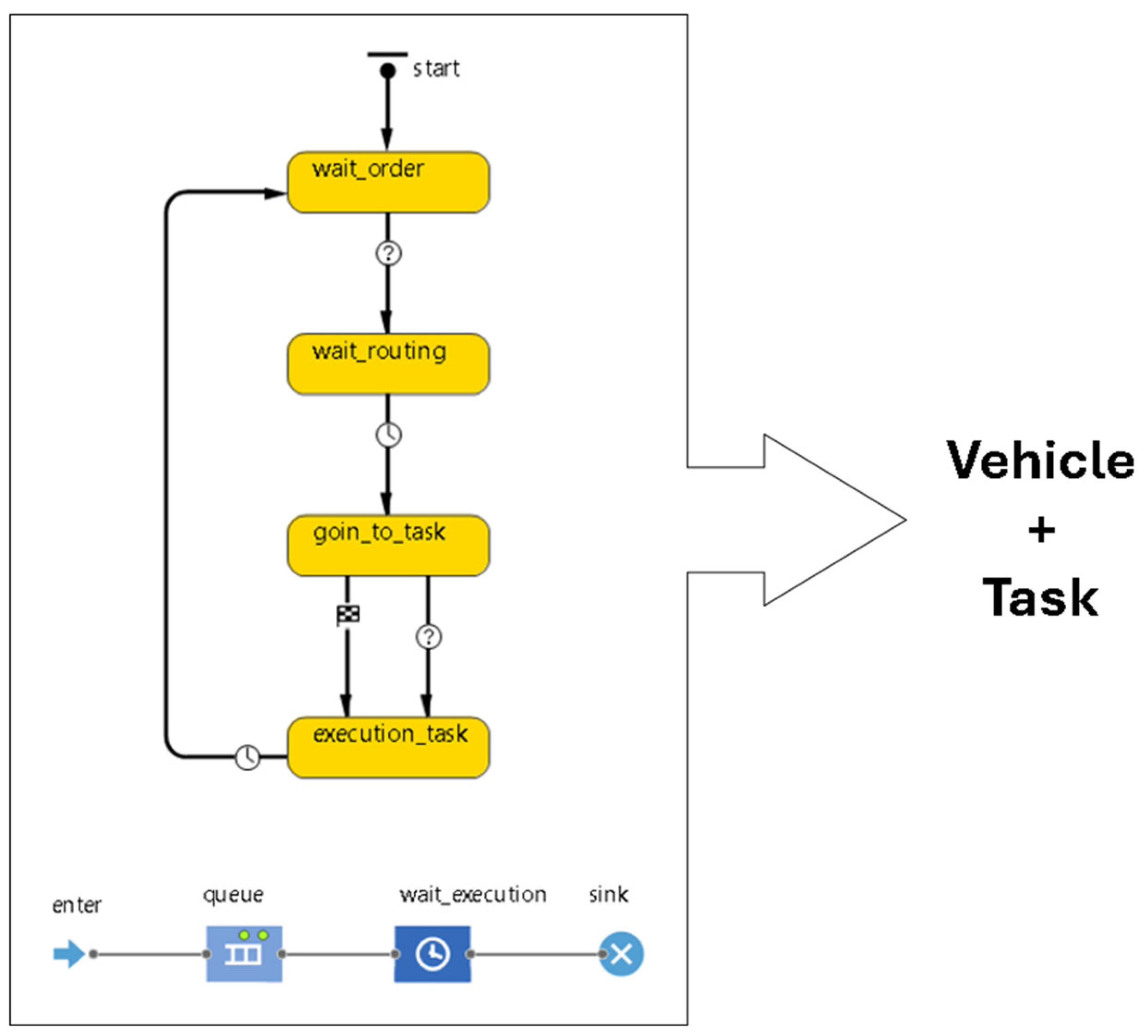
The interaction among these agents is governed by a set of behavioral rules that determine task assignment, vehicle availability, and storage decisions, aiming to optimize resource allocation and minimize costs, as shown in Figure 2. The overall workflow, from order intake to final delivery, is orchestrated using event-driven processes and queuing logic, such as the FIFO discipline for order handling. When vehicles reach their capacity or timing constraints are violated, warehouses are utilized for temporary storage, while available vehicles may serve as mobile storage units to further optimize logistics performance. This integrated modeling strategy enables a comprehensive analysis of operational strategies under both deterministic and stochastic conditions. The diagram follows the agent-based statechart and process modeling conventions of AnyLogic, inspired by UML Activity Diagram notation.

At the agent level, the operational flow begins with the wait_order state, where vehicles remain idle until a task is assigned. Once an order is allocated, the process moves to the wait_routing state, in which the routing time is calculated considering travel time variability and potential traffic delays. Subsequently, the vehicle transitions to the go_to_task state, navigating towards the pickup or delivery location according to the routing policy. Upon arrival, the execution_task state is triggered, representing the actual execution of the service, either loading or unloading the luggage. The lower process flow integrates a queue element to manage pending tasks, a wait_execution block to represent service execution time, and a sink to finalize completed operations. This combined structure allows both agent-based control (vehicle behavior) and process-based simulation (task flow management) to operate in parallel, ensuring realistic synchronization between vehicle dispatching and task execution. If additional tasks are pending, the flow returns to the wait_order state, ensuring continuous operation and efficient utilization of available resources. The integration of sequential states with queue-based process flow provides a robust framework for managing operational constraints, optimizing vehicle allocation, and minimizing idle times, while maintaining adherence to the operational rules and realistic conditions of the studied logistics scenario.

3.3. Scenario Design and Experiments

The scenario reflects the integrated operation of the MILP optimization model with the ABS environment, capturing the entire logistics process for implementation within the company in question. The application of both ABS and MILP models within the urban logistics context is illustrated in Figure 3 which depicts the integration of order processing, from the advance request of the customer order to the execution of the pickup, intermediate storage, and delivery tasks, including transshipment, storage, and contingency decisions. This flowchart demonstrates the complexity of the PDP-TW by modeling multiple agent types, vehicles, operators, and warehouses, cooperating to streamline goods movement.

This structure enables the evaluation of three distinct scenarios:

(a)

Deterministic optimal scenario—representing the MILP output without incorporating uncertainty factors in travel or task execution times.

(b)

Optimal scenario with uncertainties—extending the deterministic case by introducing stochastic variations in travel times, incident occurrence, and task execution delays.

(c)

Optimal scenario with resilience strategies—complementing the uncertainty scenario with operational buffers such as extended time windows, vehicle contingency allocation, and transshipment policies.

In all cases, the ABS implementation replicates the company’s operational rules while capturing the stochastic nature of urban logistics. Performance is evaluated using key performance indicators such as total travel time, distance travel, compliance with time windows, vehicle utilization, CO₂ emissions, and operating costs such as cost per kilometer and daily warehouse storage costs. Regarding the number of replications per scenario, a “trial and error” approach is adopted to determine an adequate sample size. This iterative process gradually increases the number of simulations until the 95% confidence intervals for the selected KPIs achieve an amplitude narrow enough to provide decision-making support. For the purposes of this study, the number of replications was fixed at 20 per scenario, ensuring statistical reliability and stability of results while avoiding unnecessary computational cost.

Initially, 10 replications were conducted for each day, and the relative half-width of the 95% confidence intervals was calculated for all KPIs. While most indicators, such as distance, travel time, execution time, and CO₂ emissions, were already within the commonly accepted 5% error threshold, the On-time rate initially exhibited higher variability on certain days. To ensure statistical robustness, the number of replications increased to 20. This adjustment significantly reduced variability across all performance indicators. With 20 replications, distance, routing time, execution time, CO₂ emissions, and the On-time rate all consistently met the 95% confidence interval requirement. Therefore, the use of 20 replications was considered statistically sufficient to ensure reliable estimation of the model’s performance indicators, balancing precision with computational feasibility. In addition, after ensuring statistical stability through 20 replications, a t-student test (paired, two-tailed) was performed to compare the performance of the PDP-TW and PDPTW-T approaches. The test confirmed statistically significant differences (p < 0.05) across all key performance indicators, validating that the improvements observed in the PDPTW-T configuration were not due to random variability.

4. Results and Discussion

In this section, the company’s real orders are used as input data to compare alternative planning scenarios rather than simulating the firm’s current operational practices. The objective is to evaluate how optimization and simulation can improve efficiency and robustness under different conditions. The mathematical models presented in Section 3.1 were coded in the Julia Programming Language, using the JuMP computational modeling package [39] and solved by Gurobi 11.0.3 [40]. The results were executed on an Intel Core i5-1035G1 1.0 GHz with 8 GB of RAM, running under Windows 11 Home Single Language (version 24H2, build 26100.6899). During the resolution of the instances, the default solver parameters were used and no execution time limit was set.

Three scenarios are analyzed. Scenario 1 represents the deterministic optimal plan generated by the MILP model, where routing and scheduling decisions are made without considering stochastic variability. Scenario 2 introduces the stochastic optimal scenario, where the deterministic plan is tested under the ABS framework, incorporating travel time uncertainty, task execution variability, and random traffic disruptions. Scenario 3 extends this analysis by applying resilience strategies whenever violations of predefined time windows are detected. These adjustments may include increasing time buffers, reallocating drivers, or adapting service priorities to maintain operational feasibility. The cost structure applied across all scenarios is based on company-provided data: EUR 0.50 per kilometer traveled and EUR 5.00 per day for temporary storage of up to 40 baggage volumes. Results are then analyzed in terms of system performance, interaction between optimization and simulation models, environmental implications in terms of CO₂ emissions, and the limitations of the proposed approach.

4.1. Case Study of Lisbon

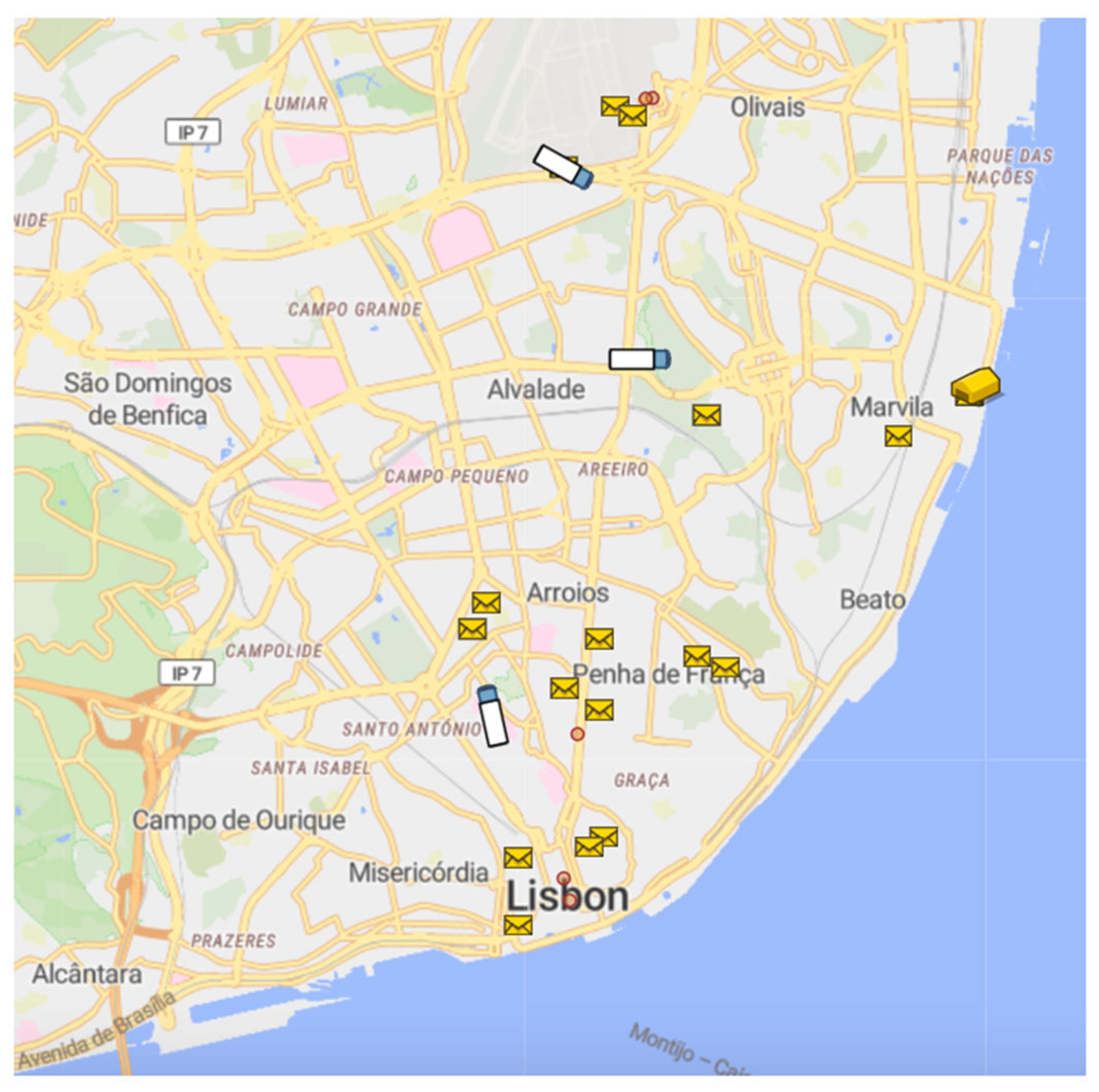
The simulation experiments were conducted in Lisbon, Portugal’s capital and largest city, located on the right bank of the Tagus River along the Atlantic coastline. This geographic position makes it the westernmost capital of continental Europe and a strategic hub for transportation and commerce. The municipality of Lisbon covers approximately 100.05 km² and forms the central core of the Lisbon Metropolitan Area (AML), which spans 18 municipalities and roughly 3015.24 km². The AML is Portugal’s most densely populated region, with nearly 3 million residents, around one-quarter of the national population, and an average population density of 956.4 inhabitants per km². Lisbon’s economic, political, and cultural significance extends across its metropolitan network, connecting with surrounding cities such as Sintra, Cascais, Almada, and Setúbal. For the purposes of this study, the simulated road network incorporated a maximum legal speed of 50 km/h, while an average operational speed of 30 km/h was adopted to reflect realistic urban driving conditions. The case company operates with a small fleet of drivers and vehicles, designated as A, B, C, etc., to handle pickup and delivery services. Vehicle allocation follows a predefined priority hierarchy established by the company, ensuring an optimized dispatch aligned with operational constraints and service objectives. Figure 4 presents the geographical area where the simulations were applied.

Figure 4 depicts the geographical layout of tasks for the day with the highest recorded order volume, focusing exclusively on the Lisbon metropolitan area, where the company concentrates its primary operations. The yellow envelope icons represent the assigned pickup and delivery tasks, the yellow warehouse symbol indicates the company’s fixed storage facility, and the truck icons correspond to the vehicles executing the routes. Additionally, the red points identify locations of simulated traffic congestion events, generated according to the uniform distribution parameters defined in the ABS model.

In Portugal, the company operates in both Lisbon and Porto, offering flexible, on-demand baggage collection and delivery services. However, the present study addresses only the operations carried out in Lisbon. Service requests can be made via the company’s mobile application, official website, or through airline ticket booking platforms. To maintain operational efficiency, customers must place orders at least two hours in advance, allowing operators to assign available drivers in accordance with a predefined priority sequence—Driver A being the first choice, followed by Driver B and Driver C, if required. On the day illustrated, corresponding to 2 January, all pre-scheduled orders from the previous day were allocated to drivers at 7:00 AM, with adjustments made during the day when necessary, while respecting both the two-hour lead time and the established driver allocation priority.

The operational constraints incorporated into the simulation include a maximum vehicle capacity of 40 baggage volumes and a driving speed profile estimated using historical data retrieved from the Google Maps API. Uncertainties affecting travel and task execution times were modelled using a triangular distribution for both route durations and handling operations, while a uniform distribution was applied to determine the occurrence of unexpected congestion incidents. When such events occur, additional delays are calculated using a triangular distribution, ensuring that both the likelihood and the impact of disruptions are realistically represented. The orders considered in the simulation correspond to empirical records of requests made at least one day in advance, in line with the company’s standard operational planning process. Within this framework, the MILP model is employed to produce more robust solutions and potentially enhance the existing task allocation strategy. It is important to highlight that demand uncertainty is not yet incorporated into the current model; only pre-scheduled orders known in advance are taken into account. Nonetheless, demand uncertainty has been addressed in prior studies, and its integration into this modelling approach remains an important avenue for future research [41,42]. This modelling framework, detailed in Section 3.1, underpins the simulation scenarios presented in this study.

Table 3. Operational records from the real system: orders, drivers, distances, and emissions.

Orders Date	Number of Tasks	Number of Drivers	Total Distance per Day (Km)	CO2 Emissions per Day	Warehouse Usage (Yes/No)
25 December 2024	1	1	16	2.03	Yes
28 December 2024	1	1	19	2.42	Yes
1 January 2025	11	2	95	12.07	Yes
2 January 2025	14	2	113	14.36	Yes
3 January 2025	13	2	98	12.46	No
4 January 2025	9	2	65	8.26	No
5 January 2025	6	2	64	8.13	No
6 January 2025	3	2	32	4.07	Yes
7 January 2025	2	1	26	3.31	No
8 January 2025	2	1	20	2.54	No
9 January 2025	6	2	61	7.75	No
10 January 2025	6	3	62	7.88	Yes
11 January 2025	3	3	30	3.81	No
12 January 2025	6	2	94	11.95	No
13 January 2025	6	2	48	6.10	Yes
14 January 2025	5	2	52	6.61	No
15 January 2025	3	2	27	3.43	No
16 January 2025	1	1	25	3.18	No
17 January 2025	5	3	46	5.85	Yes
18 January 2025	5	2	51	6.48	No
19 January 2025	4	1	45	5.72	No
20 January 2025	4	2	36	4.58	No
21 January 2025	2	2	80	10.17	No
22 January 2025	3	1	31	3.94	No
23 January 2025	3	2	40	5.08	No
24 January 2025	1	1	15	1.91	No
25 January 2025	4	1	40	5.08	No
26 January 2025	8	2	73	9.28	No
27 January 2025	3	2	30	3.81	No
28 January 2025	3	1	30	3.81	No
29 January 2025	4	1	35	4.45	No
30 January 2025	3	1	38	4.83	No
31 January 2025	8	3	85	10.80	No
Total	158	-	1622	206.1562	-

consolidates the 158 orders processed under these company operating rules in the month of January 2025, with the actual distances traveled, drivers used per day, among other relevant information.

The dataset analyzed in this study comprises 158 customer orders placed in December 2024 and January 2025. Only two orders from December were included, as their deliveries were completed in January 2025. Each order typically involves at least two tasks: a pickup and a delivery. However, certain operational characteristics required adjustments in the modeling. In particular, some orders presented inconsistencies between pickup and delivery dates, which necessitated additional interactions with the warehouse.

4.2. Iterative MILP–ABS Analysis

The integration between the MILP model and the stochastic ABS is designed as an iterative decision-support process rather than a direct performance competition. Initially, the MILP model processes the company’s daily order data to generate an optimized route plan under deterministic conditions. This solution serves as the baseline operational schedule, aiming to minimize travel distance and time while meeting vehicle capacity and time window constraints. In the subsequent stage, the ABS receives the MILP-generated plan and re-evaluates it under stochastic conditions, incorporating uncertainties such as traffic variability, incident occurrence, and handling time fluctuations. These elements are modelled using empirical probability distributions and enriched by routing data from the Google Maps API and GIS-based network representation.

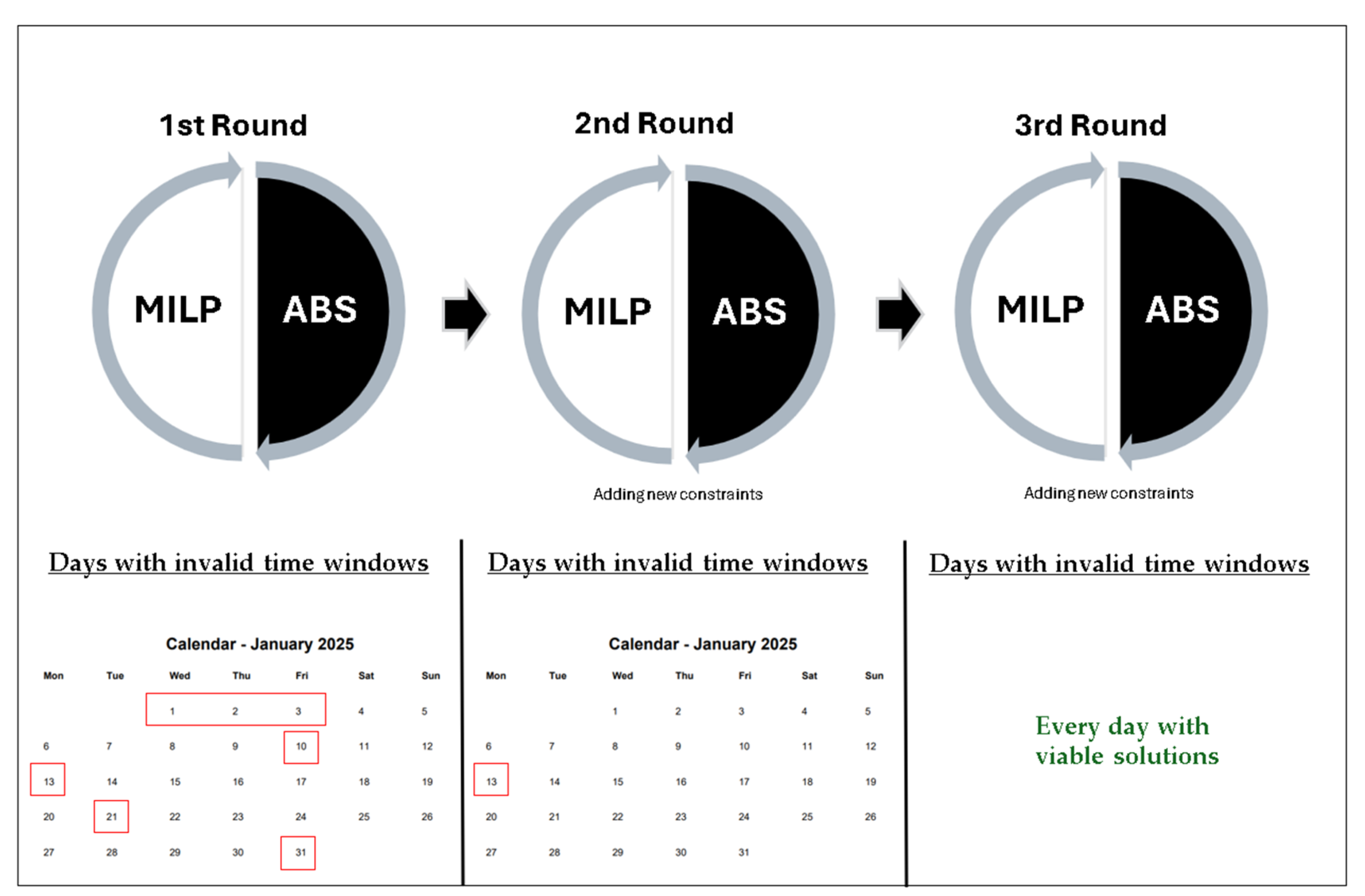
While the comparison between the deterministic and stochastic outputs highlights differences in travel times, route feasibility, and time window compliance, the primary goal is to identify operational risks and violations that may occur in real-world conditions. When such violations are detected, such as missed time windows, the feedback is sent back to the MILP model, prompting a new optimization cycle. This may involve adding constraints, adjusting time tolerances, reallocating drivers, applying cost adjustments, or introducing heuristic modifications. Figure 5 illustrates the iterative process between MILP and ABS. Each round represents a feedback loop in which infeasible solutions detected in the ABS, particularly time window violations, are reported to the MILP model. In this step, additional constraints or adjustments are introduced until all days in the planning horizon present feasible schedules.

In the first round, several days exhibited time window violations, including 1, 2, 3, 10, 13, 21, and 31 January. These cases reflect the inability of the deterministic MILP solution to fully anticipate stochastic disturbances such as traffic congestion and execution variability. Once these violations were detected by the ABS, the feedback loop allowed the MILP to incorporate corrective strategies in the second round. After adjustments, the number of problematic days was significantly reduced, with violation persisting only on 13 January. It is worth noting that the planning horizon of one month inevitably combines short-term decisions, which are executed with greater certainty and are less subject to change, with medium-term decisions that may still be adjusted. This design choice was deliberate, as it allows the hybrid framework to evaluate the robustness of solutions not only under immediate operational constraints but also across a broader planning horizon where uncertainty plays a stronger role.

Finally, in the third round, after adding further constraints and refinements to the planning process, the model reached a feasible solution for every day of the month, with no remaining violations of time windows. This iterative refinement highlights the complementary role of ABS in validating and stress-testing the MILP outcomes under uncertainty. By systematically identifying and correcting infeasibilities, the integrated framework ensures robust solutions aligned with real-world operational conditions. It is important to note that the figure does not include 25 and 28 December 2024, since these days contained only one order each (as reported in Table 3) and no time window violations occurred in the simulation.

The analysis of time window violations reveals a clear relationship between demand intensity and the occurrence of infeasibilities. With the exception of 21 January—which involved only two customer orders plus a warehouse pickup linked to an order initiated on 17 January, but nonetheless resulted in violations due to tight scheduling and long inter-node distances—all other problematic days recorded demand levels above the daily average of five orders. Notably, 1 to 3 January each exceeded 11 orders, with 2 January reaching a monthly peak of 14. Similarly, 10 and 13 January registered six orders each; on 10 January, this included a warehouse pickup related to an order from 1 January, again surpassing the average. These results indicate that higher demand intensifies route complexity and reduces available slack, thereby increasing the likelihood of time window violations. Nonetheless, the case of 21 January illustrates that even days with lower volumes can experience violations when requests are geographically dispersed or scheduled with minimal temporal flexibility.

Building on the previous results obtained for the PDP-TW, the PDPTW-T formulation was evaluated to assess the impact of introducing transshipment points into the iterative MILP–ABS integration. Figure 6 presents the procedure for January 2025, showing the rounds of interaction between optimization and simulation, as well as the identification of days with invalid time windows.

The analysis indicates that, under the PDPTW-T formulation, only 3 January initially presented time window violations during the first round of MILP–ABS integration. This infeasibility was associated with the higher number of orders on that day and the resulting tight scheduling. However, after incorporating additional constraints and executing the second round, the violations were eliminated, and all days achieved feasible solutions. These findings highlight the effectiveness of transshipment as a corrective mechanism, since it provides the necessary flexibility to absorb temporal conflicts. Therefore, the PDPTW-T approach not only reduces the occurrence of infeasibility but also ensures feasible and practical solutions even on days with atypical demand peaks.

To complement this iterative evaluation process,

Table 4. Daily performance of orders: Real operations compared with PDP-TW and PDPTW-T.

Orders Date	Nb. Orders	Number of Drivers			Total Distance per Day (Km)			Computational Time (s)		CO2 Emissions per Day (Kg)			Cost (EUR Per Km)			Warehouse Cost (EUR)
		Real	PDP-TW	PDPTW-T	Real	PDP-TW	PDPTW-T	PDP-TW	PDPTW-T	Real	PDP-TW	PDPTW-T	Real	PDP-TW	PDPTW-T
25 December 2024	1	1	1	2	16	13.59	13.59	31.141	31.141	2.03	1.727	1.727	8.00	6.80	6.80	55
28 December 2024	1	1	1	2	19	16.57	16.57	27.198	27.198	2.42	2.106	2.106	9.50	8.29	8.29	35
1 January 2025	11	2	3	4	95	74.85	70.82	277.148	359.218	12.07	9.513	9.001	47.50	37.43	35.41	45
2 January 2025	14	2	3	4	113	84.99	75.21	297.038	2531.068	14.36	10.802	9.559	56.50	42.50	37.61	75
3 January 2025	13	3	2	4	98	63.46	45.70	468.741	613.258	12.46	8.066	5.808	49.00	31.73	22.85	-
4 January 2025	9	2	2	3	65	50.31	48.75	116.831	313.011	8.26	6.394	6.196	32.50	25.16	24.38	-
5 January 2025	6	3	3	3	64	61.76	37.59	88.624	68.614	8.13	7.850	4.778	32.00	30.88	18.80	-
6 January 2025	3	2	2	3	32	21.62	29.13	80.059	69.208	4.07	2.748	3.702	16.00	10.81	14.57	25
7 January 2025	2	1	1	2	26	17.98	27.07	75.140	68.092	3.31	2.285	3.441	13.00	8.99	13.54	-
8 January 2025	2	1	1	2	20	18.80	23.31	80.091	90.097	2.54	2.389	2.963	10.00	9.40	11.66	-
9 January 2025	6	2	2	3	61	50.90	41.46	92.733	97.777	7.75	6.469	5.270	30.50	25.45	20.73	-
10 January 2025	6	3	2	4	62	56.64	22.87	91.322	120.532	7.88	7.199	2.907	31.00	28.32	11.44	35
11 January 2025	3	3	1	3	30	29.13	43.20	98.110	123.127	3.81	3.702	5.491	15.00	14.57	21.60	-
12 January 2025	6	2	2	3	94	86.75	92.97	99.541	113.385	11.95	11.026	11.816	47.00	43.38	46.49	-
13 January 2025	6	2	3	3	48	42.39	43.24	101.250	140.424	6.10	5.388	5.496	24.00	21.20	21.62	15
14 January 2025	5	2	2	3	52	41.93	40.26	88.162	103.259	6.61	5.329	5.117	26.00	20.97	20.13	-
15 January 2025	3	2	2	3	27	29.26	23.30	69.146	99.141	3.43	3.719	2.965	13.50	14.63	11.67	-
16 January 2025	1	1	1	2	25	38.29	34.64	97.028	90.055	3.18	4.867	4.403	12.50	19.15	17.32	-
17 January 2025	5	3	2	2	46	37.40	30.29	88.291	99.399	5.85	4.754	3.850	23.00	18.70	15.15	20
18 January 2025	5	2	2	3	51	44.72	34.39	92.388	110.390	6.48	5.684	4.371	25.50	22.36	17.20	-
19 January 2025	4	1	1	3	45	35.40	39.21	99.925	140.930	5.72	4.499	4.984	22.50	17.70	19.61	-
20 January 2025	4	2	2	3	36	31.86	27.95	88.183	124.879	4.58	4.049	3.552	18.00	15.93	13.98	-
21 January 2025	2	2	2	3	80	43.27	46.36	98.286	111.185	10.17	5.500	5.892	40.00	21.64	23.18	-
22 January 2025	3	1	2	2	31	22.05	32.21	80.067	100.093	3.94	2.803	4.094	15.50	11.03	16.11	-
23 January 2025	3	2	2	3	40	31.73	39.19	108.095	140.184	5.08	4.033	4.981	20.00	15.87	19.60	-
24 January 2025	1	1	1	2	15	12.62	18.61	50.921	67.088	1.91	1.604	2.365	7.50	6.31	9.31	-
25 January 2025	4	2	2	3	40	47.12	38.57	66.153	87.132	5.08	5.989	4.902	20.00	23.56	19.29	-
26 January 2025	8	2	2	3	73	64.49	59.57	61.112	81.043	9.28	8.197	7.571	36.50	32.25	29.79	-
27 January 2025	3	2	1	3	30	25.28	23.55	51.087	70.072	3.81	3.213	2.993	15.00	12.64	11.78	-
28 January 2025	3	1	2	2	30	28.10	23.53	60.870	70.139	3.81	3.572	2.991	15.00	14.05	11.77	-
29 January 2025	4	1	2	3	35	33.57	34.13	40.178	61.287	4.45	4.267	4.338	17.50	16.79	17.07	-
30 January 2025	3	1	1	3	38	29.97	35.96	80.054	100.187	4.83	3.809	4.571	19.00	14.99	17.98	-
31 January 2025	8	3	2	3	85	56.37	57.48	82.036	91.578	10.80	7.165	7.306	42.50	28.19	28.74	-
Total	158	-	-	-	1622	1343.17	1270.68	3426.949	6514.191	206.16	170.72	161.50	811.00	671.59	635.34	305

presents a descriptive characterization of the datasets associated with each scenario: Company (real operation), PDP-TW (MILP + ABS), and PDPTW-T (MILP + ABS), including transshipment as a tool. The table summarizes key operational indicators, including the number of drivers used daily, simulated daily distances, daily CO₂ emissions, costs per kilometer, and, finally, storage costs in the fixed warehouse. This characterization allows an initial comparison of the structural differences between the three scenarios prior to the performance analysis, highlighting possible variations in workload distribution and operational patterns.

The descriptive results presented in Table 4 reveal meaningful differences between the company’s real operation (Real) and the optimized planning scenario (PDP-TW). In terms of drivers, the real operation systematically uses one or two drivers per day, while the PDP-TW model demonstrates greater flexibility: on days with higher demand (e.g., 1, 2, and 3), the model assigns an additional driver to guarantee feasibility within the time windows, whereas in other situations it reduces the number of drivers compared to the real system. This result highlights the model’s ability to optimize driver utilization, not only by adding resources when necessary but also by eliminating redundancies when possible. Regarding total distance traveled, the real operation accumulated 1622 km over the month, compared to 1343.17 km under the PDP-TW scenario, a reduction of about 17.19%. The total computational time required by the optimization–simulation integration revealed a clear difference between the two models. The PDP-TW formulation required 3426.949 s (approximately 57 min), while the PDPTW-T model demanded 6514.191 s (around 1 h and 48 min). This higher processing time for the transshipment-enabled approach reflects the added complexity of coordinating vehicle routes with transfer points. Additionally, days with a higher number of orders significantly increased the computational burden for both models. For instance, 1, 2, and 3 January showed a considerable rise in solution time, with 2 January in particular registering the highest time for the PDPTW-T scenario, reaching 2531.068 s. This efficiency gain is directly reflected in the CO₂ emissions, which decreased from 206.16 kg in the real system to 170.72 kg in the optimized scenario. These improvements confirm that route optimization contributes not only to operational efficiency but also to environmental sustainability, aligning with broader policy goals for decarbonization of urban logistics.

From the perspective of costs per kilometer, the PDP-TW scenario also demonstrates advantages: the total simulated cost dropped from EUR 811 in the real operation to EUR 671.59 in the optimized plan, representing a reduction of nearly 17.19%. This effect results primarily from shorter routes and better allocation of tasks per driver. Nevertheless, the warehouse storage costs, EUR 305 across the horizon, remain an operational burden. These costs only occur in situations where temporary storage is necessary to ensure time-window compliance, a mechanism that is not explicitly accounted for in the company’s current planning. It is also important to emphasize that the variability of travel and execution times is explicitly considered in the PDP-TW results through the ABS integration. This ensures that the performance indicators reported in Table 3 already reflect the stochastic nature of urban logistics, making the comparison more realistic than a purely deterministic analysis.

Overall, the comparison between Real and PDP-TW highlights the practical benefits of optimization: shorter trip distances, reduced emissions, lower costs, and more efficient use of drivers whenever possible. However, a closer look at driver allocation reveals that the optimization process does not simply reduce resources indiscriminately; rather, it strategically adjusts them according to demand levels and spatial-temporal constraints. For example, on 1-1st and 2nd, with 11 and 14 orders, respectively, the PDP-TW model required an additional driver compared to the real system, ensuring that tight time windows at geographically distant nodes were met while achieving lower total mileage. 1-13th was the model’s most critical day, even with 6 orders, as it took three rounds to find a viable solution, which resulted in one additional driver, but with a shorter distance than the real one. Similar adjustments occurred on 1-22nd and 28th (3 requests) and on 1-29th, even with more requests (4 requests), as the proximity of time windows in dispersed locations required extra resources.

Conversely, the PDP-TW model also identified opportunities to reduce the number of drivers without compromising service quality. A particularly illustrative case occurred on 1–3rd: despite 13 orders being placed, the real system mobilized three drivers, whereas the PDP-TW consolidated routes and satisfied all requests with only two. On days with demands above or equal to the average number of orders, such as 1–10 and 31 (6 and 8 orders, respectively) and 1–17 (5 orders), the optimized solution reassigned tasks more efficiently, enabling operations with fewer vehicles than the Real system. Reductions were also observed on days with lighter demand—11 and 27 January (3 orders each), demonstrating that the model adapts to both extremes: consolidating resources when tasks are concentrated, and expanding capacity when schedules are dense or geographically dispersed.

These results highlight the model’s ability to balance operational complexity with efficient resource utilization, reducing costs without compromising service viability. Over the 33 days analyzed (two in December and the entire month of January), PDP-TW required an additional driver on 6 days (18.18%). Importantly, in all of these cases, the optimized solution still outperformed the Real system in terms of distance traveled. Conversely, on another 6 days (18.18%), the model reduced the number of drivers compared to the Real system, again with consistently lower total miles. On the remaining 21 days, the number of drivers used was equal to the Real system, in which three of these cases, PDP-TW achieved greater distances, while on the other 18, the distances were shorter. Notably, among the three days on which PDP-TW was outperformed, only 1-25th outperformed both optimized approaches, namely PDP-TW and PDPTW-T. Overall, this indicates that on 85.71% of days the PDP-TW model provided superior performance in terms of distance traveled compared to the company. These results highlight the model’s ability to balance operational complexity with efficient resource utilization, reducing costs without compromising service viability.

These results indicate that the number of daily orders alone is not the sole determinant of resource needs. Instead, the interplay between demand intensity, geographic distribution, and time-window stringency drives the adjustments made by the PDP-TW. High-order days tend to justify the addition of drivers, especially when orders are spread across distant nodes with overlapping time constraints, an aspect that strongly supports the introduction of transshipment strategies in future iterations. On the other hand, days with medium volumes (5 a 7 orders) reveal that optimization can also reduce drivers when routes and schedules are compatible. This nuanced behavior underscores that optimization entails balancing trade-offs: improving efficiency while adapting resources dynamically to operational conditions. These findings set the stage for the subsequent comparison with the PDPTW-T scenario, where transshipment mechanisms will further enhance operational resilience under uncertainty. In the PDPTW-T design, transshipment was strategically anchored at Lisbon Airport, the hub with the highest demand concentration. In this configuration, vehicles could be used as transshipment points while remaining available to perform delivery tasks. This flexibility illustrates both an operational and strategic perspective: on the one hand, the vehicles provide immediate mobile transshipment capacity; on the other, the company could establish a fixed warehouse at the airport to consolidate and redistribute flows more systematically. The modeling performed demonstrates two possible approaches to transshipment: a mobile strategy, where vehicles act as temporary hubs, and a fixed strategy, the latter being the one chosen for this study.

When assessing daily performance, exceptions can be noted. On 1–11th, the number of drivers required by the PDPTW-T coincided exactly with the real operations, while on 1–17th it was lower than the real case and equal to the PDP-TW. On 1–22nd and 28th, both PDP-TW and PDPTW-T required more drivers than the real data; however, the PDPTW-T achieved the lowest total distance on 1–28th, demonstrating how transshipment can compress routing length even when vehicle deployment increases. This trade-off reflects the dual effect of transshipment: while it may require additional resources, it simultaneously enables route consolidation and distance reduction. The cumulative results reinforce this tendency. Across the full month, the real system covered 1622 km, whereas PDP-TW reduced this to 1343.17 km and PDPTW-T further lowered it to 1270.68 km. The same pattern holds for CO₂ emissions, decreasing from 206.16 kg in the real system to 170.72 kg under PDP-TW and 161.50 kg under PDPTW-T. Regarding the cost per km, routing expenses fell from EUR 811.00 in the real case EUR 635.34 in PDPTW-T. Importantly, the benefits of PDPTW-T become most evident on days of higher demand. For days with at least six orders, the PDPTW-T consistently produced shorter total distances and lower emissions compared to PDP-TW, despite requiring an equal or greater number of drivers. This indicates that the transshipment mechanism becomes particularly advantageous under heavier workloads, where route complexity and overlapping time windows intensify operational constraints.

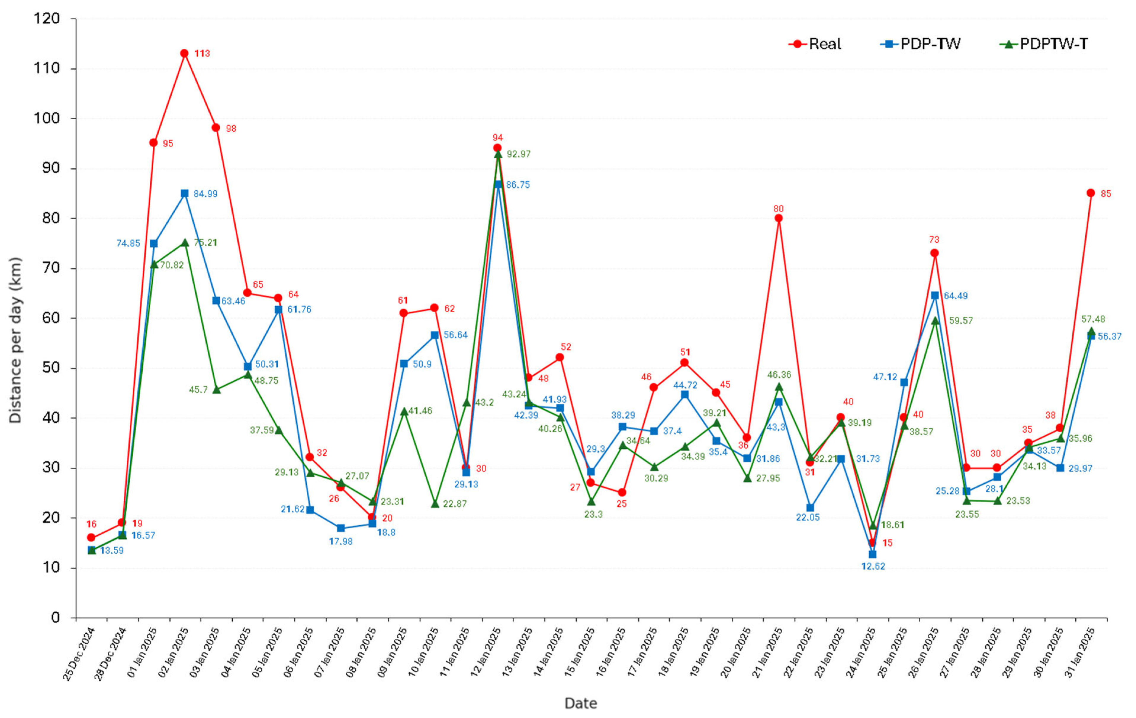
Altogether, these results underscore the strategic value of the hybrid MILP + ABS approach. By comparing alternative models, real, PDP-TW, and PDPTW-T, decision-makers can identify when the additional flexibility of transshipment justifies the deployment of extra drivers. Although the company incurs warehouse-related expenses not fully captured in this study, the explicit consideration of driver allocation shows how transshipment can simultaneously ensure service feasibility, reduce distances, and lower emissions. Therefore, the PDPTW-T strengthens the robustness urban logistics, especially during peak-demand days, and provides a data-driven foundation for adaptive decision-making in dynamic urban operations. Figure 7 shows the observed daily distances between the three scenarios (Real, PDP-TW, and PDPTW-T), showing which model achieved the shortest travel distance on each day. This comparative approach allows us to identify how transshipment mechanisms and route optimization can impact operational efficiency at different levels of demand intensity.

The analysis of Figure 7 shows that the PDPTW-T frequently achieved the shortest daily distances, particularly on days with higher order volumes. This emphasizes the role of transshipment in consolidating routes and reducing unnecessary travel under complex scheduling conditions. In contrast, the PDP-TW obtained better performance on several low-to-medium demand days, where the absence of transshipment still allowed efficient routing due to limited geographic dispersion of requests. The Real system rarely presented the best distance, with only isolated cases such as-1-16th, which underscores the efficiency gap between manual allocation and optimization-based approaches.

When the total monthly performance is considered, the Real system accumulated 1622 km, compared with 1343.17 km under PDP-TW and 1270.68 km with PDPTW-T. Furthermore, by selecting the best daily performance across all three scenarios, the total distance was reduced to just 1180.62 km. An analysis of the daily results shows that PDP-TW achieved the lowest mileage on 48.5% of the days analyzed, while PDPTW-T also outperformed on 48.5% of the days. The Real system, on the other hand, outperformed the optimized models on only 3% of the days. In addition to operational performance, this study also evaluates the environmental implications of the proposed modeling framework. Since the company’s fleet is composed of diesel-powered vehicles, travel distance is directly linked to fuel consumption and CO₂ emissions. For the estimation, a consumption rate of 0.041 L/km was adopted in combination with an emission factor of 3.1 kg of CO₂ per liter of diesel, as reported by Armenta-Déu [43]. Multiplying these values yields a composite factor of 0.1271 kg of CO₂ per kilometer traveled, which allows the direct conversion of distance into emissions. As shown in Equation (31).

$$C{O}_2 emissions\left(\mathrm{kg}\right)=Distance\left(\mathrm{km}\right)\times 0.1271$$

(31)

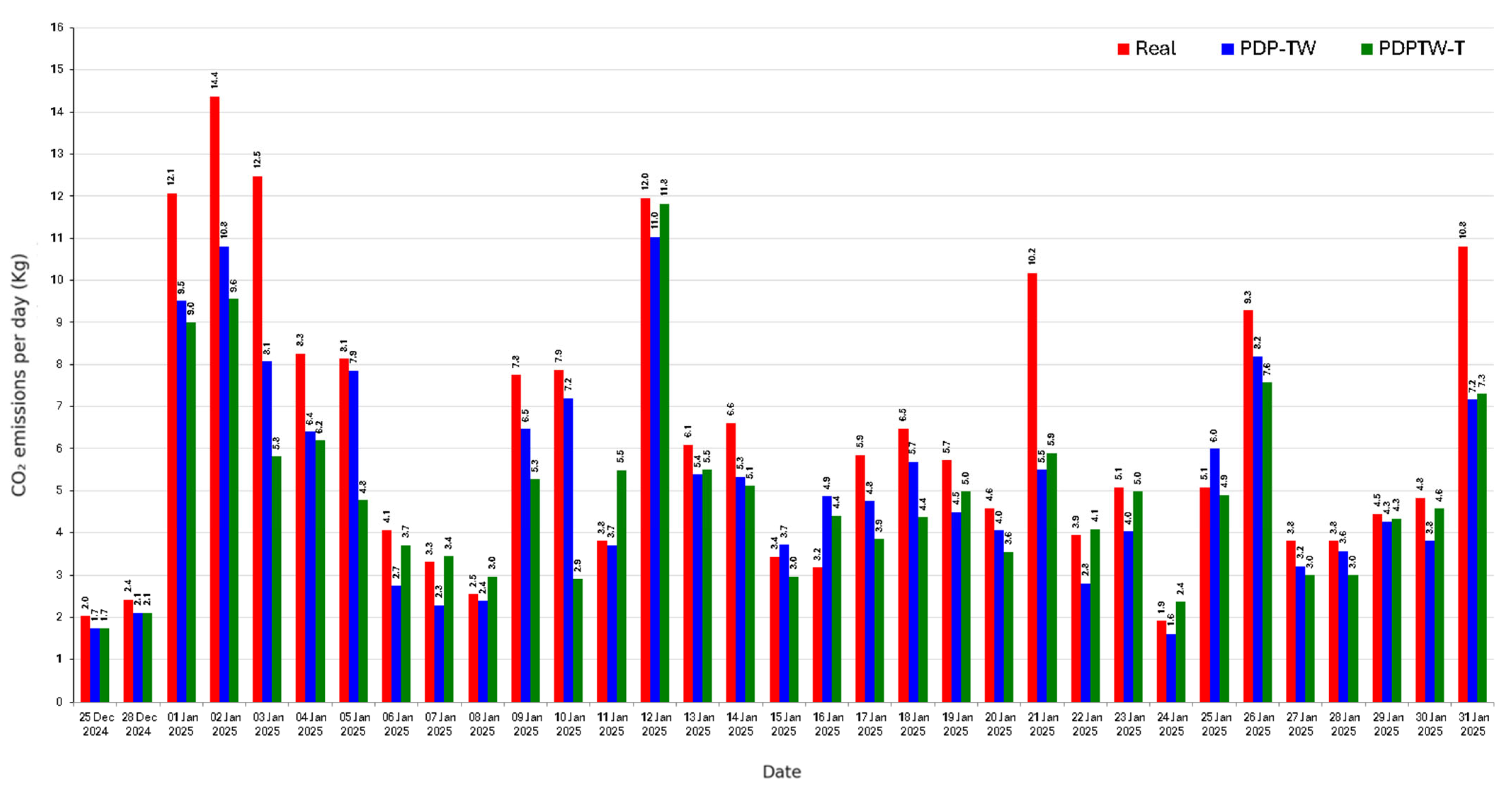
Accordingly, the improvements achieved through the integration of MILP and ABS not only reduce mileage and operational costs but also directly contribute to mitigating environmental impact. Figure 8 presents a comparative analysis of CO₂ emissions between the current operational scenario and the optimized MILP+ABS framework. The results emphasize the potential of optimization and simulation tools to support more efficient and sustainable urban logistics strategies.

Figure 8 illustrates the evolution of daily CO₂ emissions across the three scenarios. The PDPTW-T consistently reported the lowest emissions in most of-1-2025, with marked reductions compared to both the Real system and the PDP-TW baseline. This pattern directly follows the distance reductions observed in Figure 7, given the proportional relationship between kilometers traveled and fuel consumption. On days of higher demand (e.g., 1–2nd, 3rd, 10th, and 31st), the benefits of PDPTW-T were particularly pronounced, as transshipment reduced the slack in time windows and prevented excessive detours. PDP-TW performed well on several days, especially under medium workloads, but its advantage diminished in more complex routing scenarios. The Real case consistently exhibited higher emissions, reinforcing that optimization not only improves cost-effectiveness but also yields environmental benefits. These findings emphasize that integrating MILP optimization with ABS provides a strategic pathway for decision-makers to balance operational performance and sustainability objectives. From an environmental perspective, the reductions in distance directly translate into lower CO₂ emissions. Using the conversion factor listed in Equation (31) and the results in Table 4, the Real system generated approximately 206.16 kg of CO₂, while PDP-TW reduced this to 170.72 kg, and PDPTW-T further lowered it to 161.50 kg. By selecting the best daily solution across all scenarios, as shown in Figure 8, emissions dropped to only 150.05 kg, representing a potential saving of 56.10 kg of CO₂ compared with the Real operation. These results demonstrate that integrating optimization and simulation not only drives cost efficiency but also contributes to sustainability goals by mitigating the environmental footprint of urban logistics.

4.3. Discussion and Comparison Between Approaches

The iterative integration between the MILP and ABS models proposed in this study introduces a clear methodological distinction from previous hybrid frameworks. In Helo and Rouzafzoon [41], optimization and simulation were combined to support facility location and fleet sizing decisions in forestry logistics; however, the interaction occurred sequentially, without a feedback loop capable of modifying the optimization model based on simulated performance. Similarly, Muraretu and Bădică [11] employed an agent-based environment to coordinate electric vehicles through consensus mechanisms, but their optimization logic remained embedded within the agents rather than iteratively exchanging information with an external solver. Jorge et al. [44] integrated optimization and simulation for cooperative logistics but treated simulation only as a validation stage.

In contrast, the MILP–ABS feedback cycle developed in this study establishes a two-way communication between optimization and simulation, where stochastic events identified in the ABS dynamically reshape the MILP formulation, continuously strengthens the optimization process. The feedback mechanism captures time-window violations, capacity exceedances, and traffic-induced delays, translating these infeasibilities into new constraints for the next optimization run. When a violation is identified, the corresponding arcs are restricted in the mathematical model, ensuring that the new solution obtained by MILP does not visit the infeasible sequence of nodes. This adaptive cycle enables the model to progressively converge toward robust and feasible routing plans under uncertainty.

The comparative analysis between the PDP-TW and PDPTW-T configurations revealed improvements over the real system, highlighting the proposed approach for urban logistics planning. The incorporation of transshipment strategies increased operational flexibility, leading to reductions in total travel distance and time-window violations, particularly on high-demand days. These findings are consistent with previous studies by Wolfinger and Salazar-González [45], Mitrović-Minić and Laporte [46], and Avgerinos et al. [47], which have emphasized that the integration of transshipment components constitutes a powerful modeling feature with the potential to enhance operational performance, becoming increasingly beneficial as the number of daily requests grows.

To statistically validate the observed improvements, a t-student test was applied, confirming that the performance gains achieved by the PDPTW-T configuration were significant at the 5% level (p < 0.05) across all key indicators. Specifically, the PDPTW-T model achieved lower average total distance, CO₂ emissions, and operational cost, while routing and execution times, directly linked to time-window compliance, also presented significant reductions. Although the studied company does not currently implement transshipment operations, the findings suggest it could leverage its airport hub as an intermediate transfer point.

The airport is the most frequently visited node in the network, making it a strategically suitable location for consolidating and redistributing cargo. Due to data confidentiality, the company provided only aggregated cost information, assuming a fixed temporary storage cost of EUR 5 per order (within a 24 h window and up to 40 volumes), equivalent to the fixed-warehouse rate. Even under these simplified conditions, the statistical evidence underscores the practical feasibility and managerial potential of incorporating transshipment into the company’s routing strategy.

Overall, both PDP-TW and PDPTW-T consistently outperformed the real operation, except for a single low-demand day (16 January), demonstrating that the proposed hybrid MILP–ABS framework allows companies to anticipate performance variations and make robust, data-driven decisions. These results confirm that integrating optimization and ABS effectively balances routing efficiency, time-window compliance, and sustainability performance in dynamic urban contexts. The hybrid approach thus strengthens both operational planning and strategic decision-making, echoing the conclusions of Yernar and Turan [48] and Moreno et al. [2] regarding the role of iterative, simulation-based optimization in complex logistics systems.

4.4. Limitations

Despite the contributions of this study, several limitations must be acknowledged, each representing an opportunity for methodological improvement and future research development.

First, the models developed did not incorporate real-time or stochastic demand. Only pre-scheduled orders, those registered at least one day in advance—were included in the optimization and simulation. As a result, same-day requests, although feasible in practice, could not be synchronized with the MILP optimization process. Second, using MILP in the proposed framework restricts solving instances with fewer than twenty requests. Above this request count, both problems (PDP-TW and PDPTW-T) take over 8 h to find the optimal solution, making them impractical for cities with higher request volumes.

Third, the dataset used was limited to empirical records from January 2025, which constrains the generalization of results. Although 158 orders represent a relevant sample, seasonal fluctuations and peak demand variations were not captured. Fourth, the calibration of the stochastic parameters in the ABS was based on data from Lisbon, Portugal, meaning that the probability distributions and uncertainty levels are closely tied to this local context. Finally, the cost structure adopted in this study was simplified due to limited data availability. Only two components, a fixed rate per kilometer (EUR 0.50) and a daily storage fee (EUR 5), were considered.

5. Conclusions and Future Research

This study proposed a hybrid decision-support methodology that integrates optimization and ABS to address the PDP-TW under uncertainty. Using 158 real orders from January 2025 provided by a Portuguese logistics company, the methodology successfully generated optimized routing plans and validated them under stochastic conditions, bridging theoretical optimization with real-world operational complexity.

Results showed significant efficiency gains compared with the real system. The total distance was reduced from 1622 km in the real operation to 1343.17 km with PDP-TW and 1270.68 km with PDPTW-T. Selecting the best daily configuration across all models reduced distance even further to 1180.62 km. These reductions translated into concrete financial savings, lowering routing costs from EUR 811.00 in the real case to EUR 671.59 in PDP-TW, EUR 635.34 in PDPTW-T, and EUR 590.31 in the best daily solution. Environmentally, CO₂ emissions are estimated to decrease from 206.16 kg in actual operation to 170.72 kg with PDP-TW, 161.50 kg with PDPTW-T and 150.05 kg choosing the best option among the simulated scenarios. These results confirm that combining optimization with ABS not only enhances operational feasibility but also delivers measurable economic and environmental benefits.

Despite these contributions, the framework opens several promising directions for future research. Building on the current results, future studies could enhance the iterative MILP–ABS cycle through the integration of real-time demand data, adaptive learning agents, and cloud-based decision-support systems, enabling continuous re-optimization under dynamic and uncertain conditions. Furthermore, future strategies could focus on developing heuristic algorithms, expanding the scalability and practical applicability of the proposed framework.

Additionally, incorporating intra-day stochastic demand scenarios, where new pickup and delivery tasks may appear within defined time intervals, would allow the model to capture real operational variability and dynamically adjust routing decisions throughout the day. Expanding the framework to multi-city networks and incorporating a more detailed cost structure, including labor, maintenance, and environmental components, would also strengthen its managerial applicability and scalability. By advancing in these directions, the proposed hybrid methodology can evolve into a fully adaptive decision-support system for sustainable and time-constrained urban logistics operations.

References

1. Alves, R.; Lima, R.d.S.; De Oliveira, L.K.; de Pinho, A.F. Conceptual Framework for Evaluating E-Commerce Deliveries Using Agent-Based Modelling and Sensitivity Analysis. Sustainability 2022, 14, 15505. [Google Scholar] [CrossRef]
2. Moreno, R.P.; Lopes, R.B.; Ferreira, J.V.; Ramos, A.L.; Correia, D. A Study of the Main Mathematical Models Used in Mobility, Storage, Pickup and Delivery in Urban Logistics: A Systematic Review. Systems 2024, 12, 374. [Google Scholar] [CrossRef]
3. Moreno, R.P.R.; Lopes, R.B.; Ramos, A.L.; Ferreira, J.V.; Correia, D.; Melo, I.E.S. de An Agent-Based Simulation and Optimization Approach for Sustainable Urban Logistics: A Case Study in Lisbon. Appl. Syst. Innov. 2025, 8, 66. [Google Scholar] [CrossRef]
4. Han, J.; Lee, C.; Park, S. A Robust Scenario Approach for the Vehicle Routing Problem with Uncertain Travel Times. Transp. Sci. 2014, 48, 373–390. [Google Scholar] [CrossRef]
5. Srour, F.J.; Agatz, N.; Oppen, J. Strategies for Handling Temporal Uncertainty in Pickup and Delivery Problems with Time Windows. Transp. Sci. 2018, 52, 3–19. [Google Scholar] [CrossRef]
6. Xue, G.; Wang, Z.; Wang, Y. The Restaurant Delivery Problem with Uncertain Cooking Time and Travel Time. Comput. Ind. Eng. 2024, 190, 110039. [Google Scholar] [CrossRef]
7. Wang, Y.; Gou, M.; Luo, S.; Fan, J.; Wang, H. The Multi-Depot Pickup and Delivery Vehicle Routing Problem with Time Windows and Dynamic Demands. Eng. Appl. Artif. Intell. 2025, 139, 109700. [Google Scholar] [CrossRef]
8. Dridi, I.H.; Kammarti, R.; Ksouri, M.; Borne, P. Genetic Algorithm for Mulicriteria Optimization of a Multi-Pickup and Delivery Problem with Time Windows. IFAC Proc. Vol. 2009, 42, 1538–1543. [Google Scholar] [CrossRef]
9. Ma, Y.; Li, J.; Xue, J.; Li, Z. Online Crowdsourced Delivery Optimization Problem for Takeaway Orders with Balanced Rider Resources and Uncertain Travel Time. Transp. Lett. 2025, 1–20. [Google Scholar] [CrossRef]
10. Giordano, A.; Christidis, P. Green Last-Mile Delivery: Adapting Beverage Distribution to Low Emission Urban Areas. Future Transp. 2025, 5, 65. [Google Scholar] [CrossRef]
11. Murarețu, I.; Bădică, C. Optimal Agent-Based Pickup and Delivery with Time Windows and Electric Vehicles. Appl. Sci. 2024, 14, 7528. [Google Scholar] [CrossRef]
12. Romano Alho, A.; Sakai, T.; Oh, S.; Cheng, C.; Seshadri, R.; Chong, W.H.; Hara, Y.; Caravias, J.; Cheah, L.; Ben-Akiva, M. A Simulation-Based Evaluation of a Cargo-Hitching Service for E-Commerce Using Mobility-on-Demand Vehicles. Future Transp. 2021, 1, 639–656. [Google Scholar] [CrossRef]
13. Zhang, X.; Zeng, S. The Drone-Assisted Simultaneous Pickup and Delivery Problem with Time Windows. Comput. Oper. Res. 2025, 178, 106996. [Google Scholar] [CrossRef]
14. Rao, C.; Goh, M.; Zhao, Y.; Zheng, J. Location Selection of City Logistics Centers under Sustainability. Transp. Res. Part Transp. Environ. 2015, 36, 29–44. [Google Scholar] [CrossRef]
15. Lyu, Z.; Yu, A.J. The Pickup and Delivery Problem with Transshipments: Critical Review of Two Existing Models and a New Formulation. Eur. J. Oper. Res. 2023, 305, 260–270. [Google Scholar] [CrossRef]
16. Berbeglia, G.; Cordeau, J.-F.; Laporte, G. Dynamic Pickup and Delivery Problems. Eur. J. Oper. Res. 2010, 202, 8–15. [Google Scholar] [CrossRef]
17. Koç, Ç.; Laporte, G.; Tükenmez, İ. A Review of Vehicle Routing with Simultaneous Pickup and Delivery. Comput. Oper. Res. 2020, 122, 104987. [Google Scholar] [CrossRef]
18. Wang, Q.; Wu, P.; Guo, L.; Chen, P.; Ling, Y. Improving the ALNS Algorithm for PDPTW Problem Using a DDQN Agent. In Proceedings of the 2024 IEEE 13th Data Driven Control and Learning Systems Conference (DDCLS), Kaifeng, China, 17–19 May 2024; pp. 2114–2119. [Google Scholar]
19. Hu, L. Logistics Vehicle Optimization Scheduling Based on Multi Constraint PDPTW Algorithm. 5th Int. Conf. Multi-Modal Inf. Anal. MMIA 2025, 262, 438–447. [Google Scholar] [CrossRef]
20. Jun, S.; Lee, S. Evolutionary Neural Network for Learning of Scalable Heuristics for Pickup and Delivery Problems with Time Windows. Comput. Ind. Eng. 2022, 169, 108282. [Google Scholar] [CrossRef]
21. Moreno, R.P.R.; Lopes, R.B.; Ramos, A.L.; Ferreira, J.V.; Correia, D. Vosviewer-Based Bibliometric Review of Transshipment Location Problem From 2000 to 2023. Rev. Gest. Soc. E Ambient. 2024, 18, e08753. [Google Scholar] [CrossRef]
22. Rizk, Y.; Awad, M. A Quantum Genetic Algorithm for Pickup and Delivery Problems with Coalition Formation. Procedia Comput. Sci. 2019, 159, 261–270. [Google Scholar] [CrossRef]
23. Marinelli, M.; Caggiani, L.; Alnajajreh, A.; Binetti, M. A Two-Stage Metaheuristic Approach for Solving the Vehicle Routing Problem with Simultaneous Pickup/Delivery and Door-to-Door Service. In Proceedings of the 2019 6th International Conference on Models and Technologies for Intelligent Transportation Systems (MT-ITS), Kraków, Poland, 5–7 June 2019; pp. 1–9. [Google Scholar]
24. Konstantakopoulos, G.D.; Kechagias, E.P.; Gayialis, S.P.; Tatsiopoulos, I.P. Green Freight Distribution: A Case Study in Greece. In Operational Research in the Era of Digital Transformation and Business Analytics; Matsatsinis, N.F., Kitsios, F.C., Madas, M.A., Kamariotou, M.I., Eds.; Springer International Publishing: Cham, Switzerland, 2023; pp. 49–64. [Google Scholar]
25. Elbert, R.; Roeper, F. Simulation-Based Analysis of Improvements in Vehicle Routing with Time Windows Using A One-Sided VCG Mechanism for the Reallocation of Unfavorable Time Windows. In Proceedings of the 2023 Winter Simulation Conference (WSC), San Antonio, TX, USA, 10–13 December 2023; pp. 1795–1805. [Google Scholar]
26. Liu, X.; Wang, D.; Yin, Y.; Cheng, T.C.E. Robust Optimization for the Electric Vehicle Pickup and Delivery Problem with Time Windows and Uncertain Demands. Comput. Oper. Res. 2023, 151, 106119. [Google Scholar] [CrossRef]
27. Khalili-Fard, A.; Parsaee, S.; Bakhshi, A.; Yazdani, M.; Aghsami, A.; Rabbani, M. Multi-Objective Optimization of Closed-Loop Supply Chains to Achieve Sustainable Development Goals in Uncertain Environments. Eng. Appl. Artif. Intell. 2024, 133, 108052. [Google Scholar] [CrossRef]
28. Layeb, S.B.; Jaoua, A.; Jbira, A.; Makhlouf, Y. A Simulation-Optimization Approach for Scheduling in Stochastic Freight Transportation. Comput. Ind. Eng. 2018, 126, 99–110. [Google Scholar] [CrossRef]
29. Zong, Z.; Zheng, M.; Li, Y.; Jin, D. MAPDP: Cooperative Multi-Agent Reinforcement Learning to Solve Pickup and Delivery Problems. Proc. AAAI Conf. Artif. Intell. 2022, 36, 9980–9988. [Google Scholar] [CrossRef]
30. Anderluh, A.; Nolz, P.C.; Hemmelmayr, V.C.; Crainic, T.G. Multi-Objective Optimization of a Two-Echelon Vehicle Routing Problem with Vehicle Synchronization and ‘Grey Zone’ Customers Arising in Urban Logistics. Eur. J. Oper. Res. 2021, 289, 940–958. [Google Scholar] [CrossRef]
31. Malladi, S.S.; Erera, A.L.; White, C.C. Managing Mobile Production-Inventory Systems Influenced by a Modulation Process. Ann. Oper. Res. 2021, 304, 299–330. [Google Scholar] [CrossRef]
32. Ulmer, M.W.; Thomas, B.W.; Campbell, A.M.; Woyak, N. The Restaurant Meal Delivery Problem: Dynamic Pickup and Delivery with Deadlines and Random Ready Times. Transp. Sci. 2021, 55, 75–100. [Google Scholar] [CrossRef]
33. Chen, J.; Wang, L.; Wang, S.; Wang, X.; Ren, H. An Effective Matching Algorithm with Adaptive Tie-Breaking Strategy for Online Food Delivery Problem. Complex Intell. Syst. 2022, 8, 107–128. [Google Scholar] [CrossRef]
34. AnyLogic: Simulation Modeling Software Tools & Solutions for Business. Available online: https://www.anylogic.com/ (accessed on 5 April 2025).
35. Miller, C.E.; Tucker, A.W.; Zemlin, R.A. Integer Programming Formulation of Traveling Salesman Problems. J. ACM 1960, 7, 326–329. [Google Scholar] [CrossRef]
36. Attajer, A.; Darmoul, S.; Chaabane, S.; Riane, F.; Sallez, Y. Benchmarking Simulation Software Capabilities Against Distributed Control Requirements: FlexSim vs. AnyLogic. In Service Oriented, Holonic and Multi-Agent Manufacturing Systems for Industry of the Future; Borangiu, T., Trentesaux, D., Leitão, P., Cardin, O., Lamouri, S., Eds.; Springer International Publishing: Cham, Switzerland, 2021; pp. 520–531. [Google Scholar]
37. Hussein, M.; Karam, A.; Eltoukhy, A.E.E.; Darko, A.; Zayed, T. Optimized Multimodal Logistics Planning of Modular Integrated Construction Using Hybrid Multi-Agent and Metamodeling. Autom. Constr. 2023, 145, 104637. [Google Scholar] [CrossRef]
38. Abdelmageed, S.; Abdelkhalek, S.; Hussien, M.; Zayed, T. A Hybrid Simulation Model for Modules Installation in Modular Integrated Construction Projects. Int. J. Constr. Manag. 2024, 24, 1407–1418. [Google Scholar] [CrossRef]
39. Lubin, M.; Dowson, O.; Garcia, J.D.; Huchette, J.; Legat, B.; Vielma, J.P. JuMP 1.0: Recent Improvements to a Modeling Language for Mathematical Optimization. Math. Program. Comput. 2023, 15, 581–589. [Google Scholar] [CrossRef]
40. The Leader in Decision Intelligence Technology—Gurobi Optimization. Available online: https://www.gurobi.com/ (accessed on 21 October 2025).
41. Helo, P.; Rouzafzoon, J. An Agent-Based Simulation and Logistics Optimization Model for Managing Uncertain Demand in Forest Supply Chains. Supply Chain Anal. 2023, 4, 100042. [Google Scholar] [CrossRef]
42. Saprykin, A.; Chokani, N.; Abhari, R.S. Uncertainties of Sub-Scaled Supply and Demand in Agent-Based Mobility Simulations with Queuing Traffic Model. Netw. Spat. Econ. 2021, 21, 261–290. [Google Scholar] [CrossRef]
43. Armenta-Déu, C. Environmental Impact of Urban Surface Transportation: Influence of Driving Mode and Drivers’ Attitudes. Pollutants 2025, 5, 5. [Google Scholar] [CrossRef]
44. Jorge, D.; Rocha, T.; Ramos, T.R.P. A Time-Driven Simulation–Optimization Framework for the Dynamic Heterogeneous Order-Courier Assignment Problem for Instant Deliveries. Transp. Res. Part E Logist. Transp. Rev. 2024, 192, 103783. [Google Scholar] [CrossRef]
45. Wolfinger, D.; Salazar-González, J.-J. The Pickup and Delivery Problem with Split Loads and Transshipments: A Branch-and-Cut Solution Approach. Eur. J. Oper. Res. 2021, 289, 470–484. [Google Scholar] [CrossRef]
46. Mitrović-Minić, S.; Laporte, G. The Pickup and Delivery Problem with Time Windows and Transshipment. INFOR 2006, 44, 217–227. [Google Scholar] [CrossRef]
47. Avgerinos, I.; Mourtos, I.; Tsompanidis, N.; Zois, G. Pickup & Delivery with Time Windows and Transfers: Combining Decomposition with Metaheuristics. arXiv 2025, arXiv:2505.02158. [Google Scholar] [CrossRef]
48. Yernar, A.; Turan, C. Recent Developments in Vehicle Routing Problem under Time Uncertainty: A Comprehensive Review. Bull. Electr. Eng. Inform. 2025, 14, 1263–1275. [Google Scholar] [CrossRef]
Figure 1. MILP-ABS interaction for feasible solutions under uncertainty.
Computers 14 00462 g001
Figure 2. Combined Agent and Process Flow for Vehicle Routing and Task Execution.
Computers 14 00462 g002
Figure 3. Final Operational Workflow Combining MILP Optimization and ABS.
Computers 14 00462 g003
Figure 4. Spatial distribution of tasks and congestion points in the Lisbon operating area.
Computers 14 00462 g004
Figure 5. Iterative MILP–ABS integration rounds for the PDP-TW and identification of days with invalid time windows in January 2025.
Computers 14 00462 g005
Figure 6. Iterative MILP–ABS integration rounds for the PDPTW-T and identification of days with invalid time windows in January 2025.
Computers 14 00462 g006
Figure 7. Daily distance traveled: comparison between Real Operations, PDP-TW, and PDPTW-T.
Computers 14 00462 g007
Figure 8. Daily CO2 Emissions per Day (December 2024–January 2025).
Computers 14 00462 g008