A Step-by-Step Methodology for Obtaining the Reliability of Building Microgrids Using Fault TreeAnalysis

Abstract

This paper introduces an improved methodology designed to address a practical deficit of existing methodologies by incorporating circuit-level analysis in the assessment of building microgrid reliability. The scientific problem at hand involves devising a systematic approach that integrates circuit modeling, Probability Density Function (PDF) selection, formulation of reliability functions, and Fault Tree Analysis (FTA) tailored specifically for the distinctive features of building microgrids. This method entails analyzing inter-component relationships to gain comprehensive insights into system behavior. By harnessing the circuit models and theoretical framework proposed herein, precise estimations of microgrid failure rates can be attained. To complement this approach, we propose a thorough investigation utilizing reliability curves and importance measures, providing valuable insights into individual device failure probabilities over time. Such time-based analysis plays a crucial role in proactively identifying potential failures and facilitating efficient maintenance planning for microgrid devices. We demonstrate the application of this methodology to the University of Antioquia (UdeA) Microgrid, a low-voltage system comprising critical components such as solar panels, microinverters, inverters/chargers, batteries, and charge controllers.

1. Introduction

The world is currently navigating its first truly global energy crisis. This crisis began with the onset of the COVID-19 pandemic and was exacerbated by a subsequent decline in wholesale energy prices. As COVID-19 spread worldwide, the demand for gas and electricity dramatically decreased in almost every country. At the same time, an oversupply occurred due to excessive production by oil and gas companies, causing a sharp and sustained drop in energy prices. In 2022, the global energy landscape underwent a profound transformation catalyzed by the Russian invasion of Ukraine. This geopolitical upheaval triggered the most significant energy price shock since the 1970s, placing a substantial burden on the world economy. Recent estimates indicate that the portion of Gross Domestic Product (GDP) allocated to energy end-use surged from under 9% in 2020 to almost 18% in November 2022 [1]. This substantial increase has compelled governments, businesses, and various organizations to reevaluate their reliance on multinational energy sources. In response, governments and conscientious individuals are now more determined than ever to prioritize renewable resources, aiming to reduce their dependence on foreign energy supplies and fossil fuels. This collective effort underscores the global commitment to sustainable energy practices amid geopolitical and economic uncertainties.

A new alternative to meeting the sustainable energy needs of urban community loads, such as financial district buildings, universities, industrial areas, and more, is through the use of Microgrids (MGs). Microgrids are electrical systems that include multiple loads and distributed energy resources, capable of operating in parallel with the broader utility grid, thus increasing reliability, efficiency, and integration with alternative energy sources. MGs are localized energy distribution systems that incorporate renewable energy sources, such as solar panels, wind turbines, and sometimes small-scale hydroelectric generators, to supply power to a specific area or community [2]. These systems offer numerous advantages, including increased energy resilience and sustainability. By harnessing renewable sources, MGs reduce dependence on traditional fossil fuels, mitigate greenhouse gas emissions, and contribute to a cleaner environment [3]. In addition, MGs increase energy security by providing a backup power source during grid outages or disasters, ensuring that essential services continue to operate. They also promote energy independence by allowing communities to generate their electricity locally, reducing transmission losses and lowering energy costs [2,3]. Furthermore, MGs allow better integration of intermittent renewable sources, optimizing energy use and grid stability.

Nevertheless, methodologies or procedures for assessing the reliability of MGs are still under investigation. Investors, owners, and financial stakeholders in renewable energy systems should prioritize the improvement of reliability estimation methodologies. This proactive approach is vital for making well-informed investment decisions and mitigating the financial repercussions of unforeseen system failures, which could result in prolonged periods of downtime. A wide array of research papers employs diverse methodologies and models to assess reliability in MGs, encompassing holistic models, RAM analysis, Monte Carlo methodology, three-state Markov models, and Fault Tree Analysis, among others [4,5,6,7,8,9,10]. The following summary highlights some of the most pertinent approaches.

Reference [4] examines the reliability challenges and evaluation methods for grid-connected photovoltaic (PV) systems. A review of current literature reveals substantial progress in reliability assessment (RA) methodologies, reflecting the shift from conventional power generation to renewable energy sources. The fluctuating and unpredictable nature of distributed generation (DG) supporting the grid has introduced numerous new challenges, with RA being a significant one. The paper summarizes various analytical, probabilistic, simulation, and intelligent techniques employed by researchers in recent studies to assess system reliability and performance. The authors of [5] analyze how varying renewable resources and temperature affect the failure rates of renewable energy-based MGs, including wind turbines, tidal generation units, and PV systems. The study examines the impact of changes in wind speed, tidal currents, solar radiation, and air and water temperatures on key components like gearboxes, turbines, generators, electrical converters, transformers, cables, and PV panels. Both electrical and mechanical components are considered to determine an accurate, resource-based failure rate. The developed methodology and equations can be used for reliability assessments, accurately reflecting the effects of resource variations on microgrid reliability indices. However, the study lacks the application of their methodology to low-voltage (LV) systems, as described in our present work. By comparison, in [6], the authors introduce a comprehensive methodology for analyzing the availability of low-voltage DC (LVDC) systems with battery storage. It combines component reliability models, semi-Markov availability models, the Universal Generating Operator (UGO) method, and probabilistic battery reserve time analysis. This approach addresses wear-out failures and non-constant maintenance distributions of power electronic converters and offers accurate availability estimation, crucial for maintenance planning and cost considerations in LVDC systems.

The authors of [7] have developed a reliability analysis for an isolated microgrid, considering its operating conditions and the various electronic devices comprising it. This reliability analysis introduces a holistic model that incorporates multiple variables, such as irradiance and wind speed. Additionally, the paper presents a circuit model for each electronic device within the microgrid. The authors propose replacing the conventional battery energy storage system (BESS) with a hybrid energy storage system (HESS) to enhance the system’s reliability.

In Reference [8], a Reliability, Availability, and Maintainability (RAM) analysis is proposed for a PV system comprising photovoltaic modules, batteries, converters, and inverters connected to the electrical grid. This analysis tracks the evolution of RAM from subsets and groups of devices to the level of electrical subsystems. The RAM analysis is conducted by implementing reliability blocks with various photovoltaic configurations. It is concluded that the exponential Probability Density Function (PDF) is the most suitable probability distribution for the photovoltaic module, connector, and charge controller, while the Weibull PDF is optimal for the converter, bypass diode, and AC switch. In Reference [9], The authors proposed an analytical model for the sensitivity and reliability of a grid-connected PV system. This model includes sensitivity analyses conducted for a PV cell and a DC-DC converter. Additionally, the reliability models are described for each component individually using Pareto analysis [10] and logic gate representations. According to the results obtained, it was concluded that the electronic components most likely to fail are those exposed to high thermal stress, such as the switching elements (MOSFETs), due to their rapid switching speeds. However, the evolution of the reliability curve of the PV system over time is not clearly discernible. Similar to the findings of [9], the results indicate that elements such as MOSFETs or diodes, which are subject to significant thermal and voltage stress factors, tend to experience decreased reliability as these factors increase.

Fault Tree Analysis (FTA) is a powerful and widely used methodology in the field of risk assessment and reliability engineering. It provides a systematic approach to understanding and quantifying the various potential causes of a specific undesirable event. Numerous papers have been written on FTA; a brief summary of some applications in MGs follows.

The authors of [11] introduce an innovative methodology for evaluating the reliability of PV-generating systems within islanded DC microgrids, particularly under dynamic and transient operating conditions. The study begins by formulating the dynamic-voltage varying failure rate (DVVFR) and the fault-current-varying failure rate (FCVFR) of PV-generating systems in off-grid DC microgrids. The DVVFR is influenced by dynamic fluctuations in PV-source power and load power, while the FCVFR mainly accounts for failure probabilities due to various fault types in the DC microgrid. Additionally, the paper provides insights gained by comparing reliability assessment results obtained from FTA with those from Markov models and Dynamic Bayesian Network (DBN) models. In Reference [12], a reliability analysis is proposed using FTA for a microgrid operating in grid-tied mode, incorporating PV, wind turbines (WT), and BESS as distributed generators. The FTA results introduce various performance metrics, including unavailability, marginality, criticality, diagnosis, risk achievement, and risk reduction.

Reference [13] delves into the reliability assessment of DC MGs, examining two distinct configurations: ring and radial. The FTA method is employed to probe system reliability, with the aim of ensuring uninterrupted power supply to a critical AC load of 5 kW, where the loss of this load is deemed the top event of the Fault Tree (FT). For the DC ring MG, FTA is conducted using Relyence software [14], which mitigates the impact of repeated events inherent in ring configurations. Subsequently, the reliability of the DC ring MG is juxtaposed with that of the DC radial MG, focusing solely on transmission lines, through FTA analysis. However, this work lacks a documented methodology for calculating failure rates for individual electrical devices within each MG configuration.

In Reference [15], the authors propose a reliability analysis for a PV system based on an extensive dataset obtained in the field and its respective FTA. The dataset consists of collected failure rate measurements for different PV systems over a period ranging from three to five years. According to the results obtained through the FTA, inverters are identified as the components most susceptible to failure. However, the traceability of reliability over time for the analyzed PV system is not clearly observed.

In this study, our approach is based on FTA with exponential distribution, which considers the integration of battery systems, inverters/chargers, and controllers. The methodology developed in this study is applied to both military-standard data, and data extracted from the scientific literature. The utilization of military-standard data, as outlined in [11,16,17], tends to yield higher failure rate estimates than those observed in real-world scenarios. Therefore, our study can be viewed as a conservative assessment of actual failure rates, operating under the assumptions that these failures are non-repairable and components do not undergo degradation during operation. Additionally, once a component experiences a failure, the entire system is considered to be in a failure state. As a result, this paper offers a comprehensive reliability analysis of a hybrid building MG, focusing on Fault Tree Analysis. To calculate the failure rates of individual components, we employ the mathematical expressions provided in MIL-HDBK [18], with an emphasis on utilizing the exponential distribution as the probability distribution. The study also includes the estimation of reliability curves for each subsystem and electrical device, as well as for the PV system as a whole.

The rest of the paper is structured as follows: Section 2 details our step-by-step methodology for obtaining the reliability of building MGs, comprising five comprehensive steps. Section 3 presents the results, including the application of the methodology to a case study. Next, Section 4 presents the final discussion with a brief comparison with other works. Finally, Section 5 provides conclusions and highlights the findings of this research.

2. Proposed Methodology

The diagram in Figure 1 illustrates our refined step-by-step methodology, designed to effectively assess the reliability and hierarchical significance of various components within building microgrids. This comprehensive approach spans from circuit-level analysis to the identification of importance measures and minimal cut-sets through Fault Tree Analysis. Grounded in the meticulous evaluation of subsystems and electrical devices’ failure rates, this methodology draws heavily from insights gleaned from comprehensive studies outlined in [4,8,11,16,17,19,20,21].

The first step involves defining the MG and its main components. During this phase, circuit models for the devices comprising the MG are formulated. The second step requires selecting a Probability Density Function (PDF). Next, the third step involves either defining the Exponential distribution or choosing another suitable PDF. The fourth step concentrates on estimating the failure rate, also referred to as the hazard rate. Finally, the fifth step involves carrying out a Fault Tree Analysis based on qualitative analysis and quantitative analysis, comprising reliability analysis and estimation of importance measure.

2.1. First Step: Definitions of MG Circuit Models

Microgrids comprise a complex array of various components, each playing a crucial role in their functionality. These components include inverters, microinverters, photovoltaic (PV) panels, batteries, and other essential elements. During the initial phase of MG development, meticulous attention must be given to design aspects. Once the devices and their respective interconnections have been identified, the next critical step involves establishing circuit models. These circuit models act as the foundational blueprints for the MG’s electrical infrastructure, offering a comprehensive depiction of the involved components and their internal connections.

Notably, the models for the devices integrated into the MG mainly feature semiconductors, such as diodes and power switches. These semiconductor components are vital in governing the flow of electrical energy within the MG, ensuring its reliability and efficiency. A thorough understanding of these components and their interconnections is essential, as it forms the basis for subsequent stages of the proposed methodology. These later stages involve intricate analyses and assessments that are crucial in determining the MG’s performance, reliability, and overall effectiveness in meeting its intended objectives.

Below is a definition of the most common circuit models used for the equipment in energy MGs. However, it is important to note that the circuits presented here may vary among manufacturers.

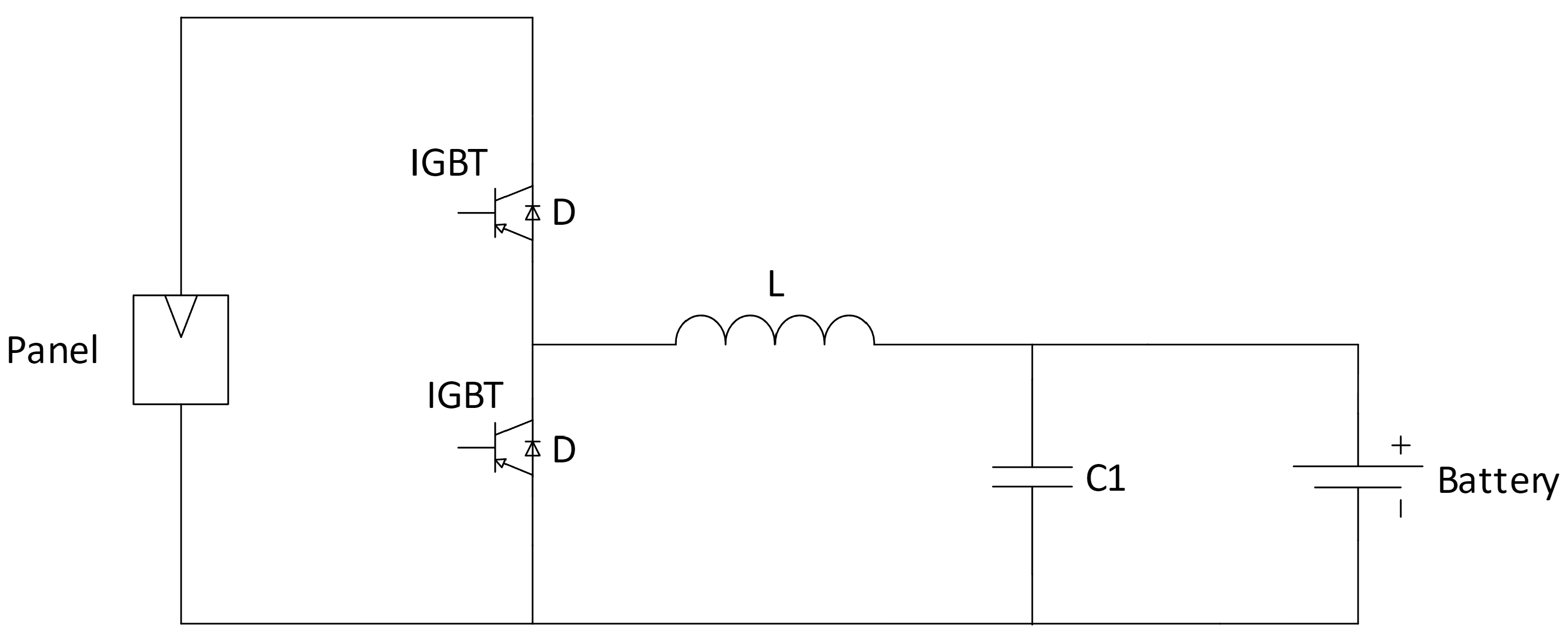
Microinverter: A microinverter is a device that converts DC power from one or more solar panels (depending on the manufacturer) to AC power. It also enables individual monitoring of each panel. Figure 2 shows the circuit model used to represent microinverters, typically consisting of an inductor, a capacitor, and five IGBTs. In this model, the microinverter corresponds to the topology of a boost converter designed to raise the input voltage to the required grid voltage.

By implementing an intelligent control strategy, such as a bipolar PWM signal at the base of the IGBTs, the inverter bridge converts the elevated DC voltage into a sinusoidal signal. This signal is then filtered for injection into the power grid when necessary [22].

Inverter/Charger: Figure 3 shows the Inverter/Charger, consisting of an inductor, three capacitors—where capacitor C1 has different characteristics from the others—and eight IGBTs. This model represents a bridge converter topology commonly used in renewable energy systems to interconnect the renewable source, storage device, and load. Typically, this model features an asymmetric control scheme for the IGBTs, aiming to achieve zero voltage switching while the switches are on, thereby minimizing circulating current losses [23,24].

Maximum Power Point Tracking (MPPT): To ensure that the PV system operates close to the maximum power point, a DC-DC converter with an MPPT controller is placed between the PV module and the load, as explained in [23]. Figure 4 shows the power stage model of a DC-DC Buck converter, which consists of an inductor, a capacitor, and two IGBTs. In PV applications, this type of converter is commonly used for charging batteries, as discussed in [25]. In such applications, maintaining a regulated current flow is crucial to prevent battery damage.

PV panels: A simplified model of a circuit equivalent to a PV cell includes a diode in parallel with an ideal current source. This current source generates current in proportion to the incident solar radiation. A more comprehensive PV cell model incorporates resistive elements to account for power losses, such as parallel leakage (or shunt) resistance, denoted as $R_{sh}$, and series resistance, referred to as $R_s$. The series resistance comprises contact resistance associated with the connection between the cell and its cables, along with the resistance of the semiconductor itself, as discussed in [26]. This model is illustrated in Figure 5.

Battery Management System (BMS): The BMS is a power electronic system that intelligently manages the charge and discharge of the battery cells, thus preventing accelerated wear. The BMS allows balancing the battery cells in such a way that all cells are charged and discharged at the same time, increasing the lifespan of the device and ensuring complete charging and discharging of the battery pack. Figure 6 illustrates a Buck–Boost converter topology commonly employed in BMS [27]. It is worth noting that BMS topology is highly diverse and depends on the design of each manufacturer.

Battery: This is a device that stores electrical energy for later use. Batteries provide a greater degree of freedom to microgrids, allowing for efficient energy management. Excess energy can be stored in the battery to be used later when the load requires it or when generation is unavailable.

Batteries exhibit high diversity, commonly utilizing electrolytes of various chemistries, including lead-acid, cadmium, nickel, and lithium, among others. Due to the wide variety and complex construction characteristics of these systems, obtaining failure rates is beyond the scope of this research work. Therefore, it is recommended to consult the failure rates directly from the manufacturer’s website or from other researchers who have reported the information. Because a battery is an electrochemical element, it does not usually present a circuit model useful for our analysis. However, it is considered as a device with a specific failure rate [28].

2.2. Second Step: Selection of a Probability Density Function

To predict the reliability of an electronic component, it is first necessary to select a Probability Density Function (PDF) that is suitable for failures occurring in electrical or electronic components, so that the real probability density function should be derived from experiments like Accelerated Life Tests (ALTs), with Log-normal, Binomial, Weibull, or mixed-Weibull distributions being the likeliest outputs.

Although the exponential distribution is not necessarily the correct distribution for failures in these components [4,6], our analysis employs this distribution. This is because, in most reliability databases, the failure rate of electronic systems is considered constant and represented by $\lambda$.

Conversely, other characteristic parameters of a probability distribution, such as the Weibull scale and shape factors, are less commonly found in the scientific literature and datasheets. Nonetheless, changing the function from exponential to a different one is not a big issue, as if the implementation of this method stays the same while ALTs are run to correctly estimate PDFs, should be considered as a fundamental step to obtain realistic reliability estimates [29].

2.3. Third Step: Exponential Distribution

The continuous probability distribution $f\left(t\right)$ can be employed to describe the useful life of a device, with several life distributions used in reliability analysis. Typically, the exponential distribution is widely employed in reliability analyses due to its applicability to various systems and its mathematical simplicity. In this paper, we opt for the exponential distribution as it aligns well with the failure patterns observed in many electronic devices. This choice is supported by findings discussed in references [4,19,21,30] which highlight the prevalence of exponential failure behavior in electronic components and systems.

Electronic devices often exhibit failure rates that decrease over time, a characteristic that closely resembles the exponential distribution’s PDF. This distribution is particularly suitable for modeling systems with a constant hazard rate, making it a natural choice for reliability studies in electronics.

Given the widespread adoption of the exponential distribution in reliability engineering, our decision to utilize it in this paper is further reinforced by its established relevance and applicability to electronic systems. This choice ensures consistency with industry standards and facilitates comparisons with existing literature on reliability modeling in electronic devices.

Therefore, a random variable T follows the Exponential distribution if and only if its PDF is as follows:

$$f\left(t\right)=\lambda e^{-\lambda t},t\ge 0$$

(1)

In this context, the failure rate function, denoted as $\lambda \left(t\right)=\lambda$, represents a constant parameter that can be determined through tests specific to a particular device or derived from historical data previously collected for reliability analysis. This failure rate is typically defined in terms of failures per hour, and can be calculated as follows:

$$\lambda =\frac{\mathrm{Number}\mathrm{of}\mathrm{failures}}{\mathrm{Total}\mathrm{operating}\mathrm{hours}}$$

(2)

2.4. Fourth Step: Failure Rate Estimation

According to the circuit models for the microinverter, Inverter/Charger, MPPT, PV cell, and BMS presented in Section 2.1, it is possible to determine the constant failure rate of each of these devices. To estimate its failure rate, we use the methodology proposed in the MIL-HDBK-217 Manual [18]. The use of military-standard data, as outlined in references [11,16,17], tends to yield higher failure rate estimates than those observed in real-world scenarios. These military standards are used precisely because of their conservative nature and their ability to ensure an adequate safety margin.

This manual provides failure rates ${\lambda }_b$ for electronic devices, where the actual failure rate $\lambda$ is calculated as indicated in [31]:

$$\lambda ={\lambda }_b\left(\prod _{i=1}^n{\pi }_i\right)$$

(3)

where n is the number of $\pi$ factors of the device that consider the stresses.

Thus, this manual estimates the lifetime of each element that composes a certain device, in order to estimate the average lifetime of the device. In this way, the expressions given below are used to determine the failure rate of the following components:

$$\begin{array}{}\mathrm{(4)}& {\lambda }_{IGBT}={\lambda }_b{\pi }_T{\pi }_S{\pi }_A{\pi }_R{\pi }_Q{\pi }_E\hfill \mathrm{(5)}& {\lambda }_{Diode}={\lambda }_b{\pi }_T{\pi }_S{\pi }_C{\pi }_Q{\pi }_E\hfill \mathrm{(6)}& {\lambda }_{Capacitor}={\lambda }_b{\pi }_T{\pi }_C{\pi }_V{\pi }_{SR}{\pi }_Q{\pi }_E\hfill \mathrm{(7)}& {\lambda }_{Inductor}={\lambda }_b{\pi }_T{\pi }_Q{\pi }_E\hfill \end{array}$$

where ${\lambda }_b$ is the base value of the failure rate. The temperature factor $\left({\pi }_T\right)$ can be calculated using the adequate expression for every component [17]. The voltage stress factor $\left({\pi }_S\right)$ is used for the calculation of the failure rate of semiconductor devices and depends on the nominal voltage of the device indicated in [32]. The capacitive factor $\left({\pi }_C\right)$ is used for the calculation of the capacitor failure rate and depends on the value of the capacitance $\left(C\right)$, which is expressed in microfarads [17]:

$${\pi }_C=C^{0.23}$$

Conversely, the nominal power factor $\left({\pi }_{SR}\right)$ depends on the rated voltage of the capacitor. Finally, stress factors such as the application factor $\left({\pi }_A\right)$, the quality factor $\left({\pi }_Q\right)$, and the environmental factor $\left({\pi }_E\right)$ are obtained from the manual, depending on the component’s use. To determine the failure rate of any device, the different failure rates of its components are added up, so when a device contains multiple components of the same type, their respective failure rates are multiplied by the number of such components. The following subsections detail failure rates for the typical devices that are installed in Building MGs.

2.5. Fifth Step: Fault Tree Analysis

The purpose of this paper is to evaluate the reliability of building MGs and understand their degradation over time. This assessment is conducted using Fault Tree Analysis (FTA). This is a systematic method used for identifying and analyzing potential causes of system failures, however, like any method, it has its own strengths and weaknesses.

Advantages of Fault Tree Analysis:

(1) Systematic Approach: FTA provides a structured and systematic approach to analyzing potential failures within a system, ensuring that all possible causes are considered. (2) Visual and Clear: FTA uses a diagrammatic approach, making it easy to understand the relationships between failures and the undesired top event. This clear picture helps communicate complex ideas to a wider audience. (3) Early Detection of Failure Modes: FTA can be used during the design phase of a system to identify potential failure modes early in the development process, enabling design improvements to enhance system reliability. (4) Decision Support: FTA provides valuable insights that can aid decision-making regarding system design, maintenance strategies, and resource allocation to mitigate risks effectively.

Disadvantages of Fault Tree Analysis:

(1) Complexity: FTA can become complex, especially for large and complex systems, leading to difficulties in accurately modeling all potential failure modes and their interactions. (2) Data Dependence: FTA can be used quantitatively to assess risk, but this requires reliable data on failure rates and probabilities. In some cases, such data may be unavailable or difficult to estimate accurately. (3) Foresight Needed: FTA requires anticipating the potential failures that could lead to the undesired event. If a critical failure mode is missed, the analysis may not be effective. (4) Limited Scope: FTA typically focuses on a single undesired event, while it can explore various causes, it might not capture the full range of potential issues within a system. Furthermore, it may not address other aspects of system performance, such as performance degradation over time or human factors.

Notwithstanding those disadvantages, this method has been successfully applied in various instances to achieve reliability and safety evaluation objectives, as cited in [11,12,13,33,34,35].

An FT model is indeed valuable for comprehending the behavior of complex systems by analyzing the relationships between the individual components that collectively constitute the entire system. This model employs a tree structure composed of events and logic gates. Events represent both normal conditions and system failures (including component failures, environmental conditions, human errors, and others) and implement Boolean logic, enabling them to be either false or true. Conversely, logic gates represent cause–effect relationships between events. The top event defines the system’s failure mode or its function, which is then examined in terms of the failure modes of its components and related factors, as discussed in [36]. Consequently, one of the major advantages of FTA is its ability to predict most individual failures leading to a complete system breakdown.

A gate input can consist of either a single event or a combination of events originating from the output of another logic gate, as discussed in [37]. Additionally, various types of gates are available within the formalism, including $AND$, $OR$, and K-out-of-N gates.

$AND$ Gate: the logical $AND$ gate represents the condition when a combination of basic events must occur to produce a certain output event. In this case, such an output event describes a failure. In terms of probability this would be:

$$F(A\cap B\dots \cap N)=F\left(A\right)·F\left(B\right)·\dots ·F\left(N\right)$$

(8)

$OR$ Gate: the logical $OR$ gate represents the condition when at least one basic event must occur to produce a certain output event. In terms of probability this would be:

$$F(A\cup B\dots \cup N)=1-[1-F(A\left)\right]·[1-F(B\left)\right]·\dots ·[1-F(N\left)\right]$$

(9)

K-out-of-N Gate: the K-out-of-N gate, or voting gate, represents the condition where the output is enabled if at least K inputs/events have occurred. In addition, in the FT model, the rectangles indicate middle events, or by default, the top event when at the top of the FTA. These events occur in case the input conditions are met in one or more logic gates. The circles (input conditions for gates) represent basic events that are generally associated with the probability of device failure. These elements are shown in Figure 7.

In terms of evaluation, FTA is an effective technique for both qualitative and quantitative assessments of system reliability and availability, as highlighted in [38] and briefly described in the following subsections.

2.5.1. Fifth Step (A): FTA Qualitative Analysis

This refers to the assessment and analysis of system failures without assigning specific numerical values to the probabilities of events. Qualitative analysis is often the initial step in the FTA process, providing a conceptual understanding of the system’s failure modes. This precedes quantitative analysis, where specific probabilities are assigned to events and calculations are made to assess overall system reliability. This qualitative approach is valuable when precise quantitative data may be scarce or when a broad understanding of the system’s vulnerabilities is needed [35].

In qualitative analysis, a cut-set is a combination of basic events or failure modes whose occurrence leads to the top event or system failure. A cut-set represents a path through the FT, illustrating how the failure of certain components or events can contribute to the overall failure of the system.

Conversely, minimal cut-sets refer to the smallest combinations of system components or events whose simultaneous failure can cause the system to fail. When a event is removed from a minimal cut-set, the remaining events still contribute to the likelihood of system failure because there is still a path from each basic event to the top event. By understanding and addressing minimal cut-sets, engineers and analysts can focus on the most critical elements contributing to the MG system failure, allowing for targeted improvements to enhance overall system reliability and safety.

2.5.2. Fifth Step (B): FTA Quantitative Analysis

Quantitative Analysis in the context of FTA and reliability engineering involves assigning numerical probabilities to events and calculating the probability of the top-level event or system failure. Thus, this analysis provides a more precise assessment of system reliability by incorporating quantitative data. The key aspects of Quantitative Analysis in FTA include the following [35]:

Probability Assignments: Each basic event or failure mode in the FT is assigned a probability of occurrence. These probabilities are often based on historical data, expert judgment, or other sources of information. Cut-set Probability Calculation: The probability of is determined by treating the events within the cut-set as if they were all linked by an $AND$ operation. Put differently, for a cut-set comprising events A, B, and C, its probability is calculated as $Pr$(A $AND$ B $AND$ C), which is equivalent to multiplying the probabilities of A, B, and C individually $\left(Pr\right(A)\ast Pr(B)\ast Pr(C\left)\right)$ due to the independence of the basic events.

Top Event Probability: The final step involves calculating the overall probability of the top-level event or system failure. This is typically done by summing the probabilities of all minimal cut-sets. However, this can be overly conservative because it assumes all cut-sets are completely independent. To account for overlapping events, more advanced methods consider the probability of intersections between minimal cut-sets and subtract them accordingly.

Quantitative Analysis offers a precise assessment of system reliability, aiding in informed decision-making for risk mitigation, system improvements, and resource allocation. This is crucial for complex systems like grid-connected PV systems, where understanding each component’s contribution to overall failure is essential.

Reliability Analysis

Reliability is defined as the probability that the system, subsystem, or components perform their required function adequately in the interval $[0,t)$, such that, the Probability Density Function (PDF), $f\left(t\right)$, represents the failure distribution of the population of components over the entire time range [8,29].

In addition, the failure probability function $F\left(t\right)$ is the probability that a component fails in a specified time t, and it is defined as the Cumulative Distribution Function (CDF) of the PDF, where T is a random variable that represents the time to failure of a system component [29]:

$$F\left(t\right)=\mathrm{Pr}(T\le t)={\int }_{-\infty }^{t}f\left(t\right)dt$$

(10)

Therefore, the reliability probability function $R\left(t\right)$ indicates the fraction of the population that survives at time t, and it is derived from Equation (10) knowing that it is the 1’s complement of $F\left(t\right)$:

$$R\left(t\right)=1-F\left(t\right)=\mathrm{Pr}(T>t)={\int }_t^{\infty }f\left(t\right)dt$$

(11)

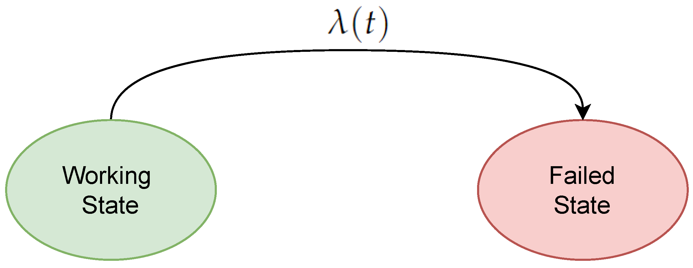
Without losing generality, it can be assumed that a system has two states [21], as shown in Figure 8. The transition from the working state to the failed state is initiated by the failure rate function $\lambda \left(t\right)$. This function represents the rate of change in the probability that a surviving product will fail in the next small-time interval and is expressed as:

$$\lambda \left(t\right)=\frac{f\left(t\right)}{1-F\left(t\right)}$$

(12)

The Mean Time To Failure (MTTF), which signifies the expected useful life of a component, is the most common method for specifying the reliability of non-repairable items, as discussed in [28]. It can be calculated as follows:

$$MTTF={\int }_0^{\infty }t·f\left(t\right)dt={\int }_0^{\infty }R\left(t\right)dt$$

(13)

Under these circumstances, and considering the Exponential Distribution in Equations (11) and (12), the reliability $R\left(t\right)$ would be described as:

$$R\left(t\right)=e^{-\lambda t}$$

(14)

Such that, by using Equation (13), MTTF would be:

$$MTTF=\frac{1}{\lambda }$$

(15)

Importance Measures

Importance measures quantify how individual components affect a system’s reliability and performance. They are vital in reliability analysis, helping understand component importance and informing decisions on maintenance, design enhancements, or system upgrades. By pinpointing critical components, engineers optimize resource allocation, improving overall system reliability and performance.

There are various importance measures used in reliability engineering, including but not limited to [39]:

Marginal Importance:

This assesses how a small change in a component’s reliability impacts the overall system reliability or performance. A high marginal importance indicates that boosting the reliability of that component would greatly improve the system’s performance.

If E is the top event of a system, and A is another component, then the marginal importance measure is the difference between the probability of E given that A did occur (probability of event A is set to 1), and the probability of E given that A did not occur (probability of event A is set to 0). So,

$$\mathrm{Marginal}\mathrm{Importance}=\mathrm{Pr}\left(E\right|\mathrm{Pr}\left(A\right)=1)-\mathrm{Pr}(E\left|\mathrm{Pr}\right(A)=0)$$

(16)

This importance measure allows the increase in the probability of E given the occurrence of A to be seen.

Criticality Importance:

This assesses a component’s influence on critical system functions or performance. Components vital for system functions or safety have high criticality importance. Identifying these crucial components is key for prioritizing maintenance and ensuring system reliability. Mathematically, it takes the Marginal Importance measure, and multiplies it by the probability of A divided by the probability of E.

$$\mathrm{Criticality}\mathrm{Importance}=(\mathrm{Marginal}\mathrm{Importance})\ast \frac{\mathrm{Pr}\left(A\right)}{\mathrm{Pr}\left(E\right)}$$

(17)

Diagnostic Importance:

This gauges how much a component aids system diagnostics. In systems reliant on diagnostics, specific components significantly enhance fault detection and identification. Diagnostic importance pinpoints components that, if monitored or tested, can bolster the system’s fault detection and isolation capabilities. It can be calculated as the fraction of the probability of the top event E that includes the occurrence of event A:

$$\mathrm{Diagnostic}\mathrm{Importance}=\frac{\mathrm{Pr}\left(A\right)}{\mathrm{Pr}\left(E\right)}\ast \mathrm{Pr}\left(E\right|\mathrm{Pr}\left(A\right)=1)$$

(18)

Risk Achievement Importance (RAI):

This evaluates how a component influences achieving a set risk level in the system, commonly utilized in risk assessment and safety-critical systems. Components with high risk achievement importance greatly contribute to reaching an undesired level of risk if they fail. Managing and mitigating the risk associated with these components becomes a priority. Specifically, it reports the ratio between the probability of E when event A is given to occur (probability of event A is set to 1), and the probability of E:

$$\mathrm{RAI}\mathrm{Measure}=\frac{\mathrm{Pr}\left(E\right|\mathrm{Pr}\left(A\right)=1)}{\mathrm{Pr}\left(E\right)}$$

(19)

Risk Reduction Importance (RRI):

This measures how much a component decreases system risk when its reliability improves. Identifying components with significant risk reduction importance is crucial for prioritizing effective risk mitigation strategies. It can be calculated as the reduction in the probability of top event E when event A is given to not occur. So, it would be the ratio between the probability of E, and the probability of E when event A is given to not occur (probability of event A is set to 0):

$$\mathrm{RRI}\mathrm{Measure}=\frac{\mathrm{Pr}\left(E\right)}{\mathrm{Pr}\left(E\right|\mathrm{Pr}\left(A\right)=0)}$$

(20)

These various importance measures provide nuanced insights into different aspects of an MG system’s reliability and performance, aiding engineers and analysts in making informed decisions for MG design, maintenance, and risk management.

3. Results

The system analyzed in this work is a low-voltage hybrid building MG consisting of several electronically controlled distributed resources connected in parallel, designed to operate in both islanded and grid-connected modes. The system operates at 208 $V_{AC}$ with 20 kW of real installed solar power. Please see Figure 9.

This microgrid is located at the Eastern Campus of the University of Antioquia (Colombia) and has been specifically implemented in Building 3 of the campus. It can be disconnected from the utility power grid and continue to operate during power outages, drawing power from on-site PV and energy storage systems with batteries. The primary load supplied by this microgrid is the building’s lighting system.

Figure 10 presents a single-line diagram of the UdeA Microgrid. It is composed of 30 PV panels (Q.peak-G5 315 W manufactured by Q cell in Germany), 27 microinverters (IQ7+ manufactured by enphase in China), an MPPT controller (MPPT 75/15 manufactured by Victron in Germany), four batteries in parallel (US3000C manufactured by Pylontech in China), and three single-phase inverters configured within a three-phase inverter/charger (Quattro 5 kW manufactured by Victron in Germany).

The diagram illustrates two essential buses: the Direct Current Bus (DC Bus) and the Three-Phase Alternating Current Bus (3$\mathrm{\Phi }$ AC Bus). The MPPT controller manages three PV panels, optimizing their power output. The three-phase inverter/charger facilitates the connection and disconnection of the power grid and regulates the power load. The system includes 27 microinverters, distributed with 9 microinverters per phase, each dedicated to a single panel. These microinverters are connected to the AC bus, which also supplies the load.

3.1. Circuit Model Definitions and Selection of the PDF

As seen in the previous sections, the first three steps of our methodology pertain to theoretical aspects of circuit modeling and the selection of the PDF that will be used in the reliability analysis of the microgrid under study.

Results of applying the First step—Definitions of MG Circuit Models:

The MG under study is primarily composed of 27 microinverters, an inverter/charger, an MPPT controller, 30 PV panels, a BMS, and four batteries. The first step of our methodology then involves using the circuit models referenced in Section 2.1 to estimate the failure rate of each component. This estimation is followed by assessing the corresponding reliability, as detailed in the subsequent steps of the proposed methodology.

Results of applying the Second and Third steps—Selection of the PDF:

As described in Section 2.2, our methodology employs the exponential distribution as the PDF to model the useful life of the electronic devices in our hybrid building MG. This choice implies that the failure rate function is represented by a constant $\lambda$, defined in terms of failures per hour. For more details on selecting the PDF and the application of the exponential distribution to electronic components, please consult Section 2.2 and Section 2.3.

3.2. Results of Applying the Fourth Step: Failure Rate Estimation

Following the step described in Section 2.4, the present section includes results concerning the failure rate estimation for the various components that compose the MG under study.

Table 1. Failure rates of Microinverter Components.

	IGBT	Diode	Capacitor	Inductor
${\lambda }_b$	0.00074	0.005	0.00012	0.00003
${\pi }_T$	1.40	1.64	1.92	1.23
${\pi }_S$	0.42	0.55	-	-
${\pi }_A$	0.79	-	-	-
${\pi }_R$	8.25	-	-	-
${\pi }_Q$	5.50	5.50	10	3
${\pi }_E$	6	6	6	6
${\pi }_C$	-	1	5.87	-
${\pi }_V$	-	-	4.48	-
${\lambda }_{\mathit{total}}$	$9.00\times {10}^{-8}$	$1.50\times {10}^{-7}$	$3.60\times {10}^{-7}$	$6.64\times {10}^{-10}$

shows the different values of the failure rates of each microinverter component, determined from Equations (4)–(7), such that the $\pi$ factors were obtained from a combination of real-world observations (empirical data) and theoretical models outlined in the MIL-HDBK-217 handbook [18].

Based on the number of components shown in Figure 2, the microinverter failure rate can be written as:

$${\lambda }_{Microinverter}=5·{\lambda }_{IGBT}+{\lambda }_{Capacitor}+6·{\lambda }_{Diode}+{\lambda }_{Inductor}$$

(21)

Substituting the values from Table 1 in Equation (21), it is obtained that the failure rate for the microinverter is 1.71 × ${10}^{-6}$ [failure/hour].

In the same way that the failure rate is calculated for each microinverter component, the failure rate is calculated for each component of the Inverter/Charger.

Table 2. Failure rates of Inverter/Charger Components.

	IGBT	Diode	Capacitor C1	Cap. C2, C3	Inductor
${\lambda }_b$	0.00074	0.005	0.00012	0.00012	0.00003
${\pi }_T$	1.40	1.64	1.92	1.92	1.23
${\pi }_S$	0.42	0.15	-	-	-
${\pi }_A$	0.79	-	-	-	-
${\pi }_R$	16.89	-	-	-	-
${\pi }_Q$	5.50	5.50	10	10	3
${\pi }_E$	6	6	6	6	6
${\pi }_C$	-	1	5.87	6.89	-
${\pi }_V$	-	-	1.01	1.27	-
${\lambda }_{\mathit{total}}$	$1.90\times {10}^{-7}$	$4.00\times {10}^{-8}$	$8.00\times {10}^{-8}$	$1.20\times {10}^{-7}$	$6.64\times {10}^{-10}$

shows the different failure rates for these components. Here, the $\pi$ factors were also obtained from a combination of empirical data and theoretical models outlined in the MIL-HDBK-217 handbook [18].

According to the number of components shown in Figure 3, the Inverter/Charger failure rate can be written as:

$${\lambda }_{\mathit{Inverter}/\mathit{Charger}}=8·{\lambda }_{IGBT}+{\lambda }_{C1}+2·{\lambda }_{C2}+8·{\lambda }_{Diode}+{\lambda }_{Inductor}$$

(22)

Replacing the values from Table 2 in Equation (22), it is obtained that the failure rate of the Inverter/Charger is $2.16\times {10}^{-6}$ [failure/hour].

Table 3. Failure rates of MPPT Components.

	IGBT	Diode	Capacitor	Inductor
${\lambda }_b$	0.00074	0.005	0.00012	0.00003
${\pi }_T$	1.40	1.64	1.92	1.23
${\pi }_S$	0.42	0.15	-	-
${\pi }_A$	0.79	-	-	-
${\pi }_R$	12.88	-	-	-
${\pi }_Q$	5.50	5.50	10	3
${\pi }_E$	6	6	6	6
${\pi }_C$	-	1	5.87	-
${\pi }_V$	-	-	4.48	-
${\lambda }_{\mathit{total}}$	$1.50\times {10}^{-7}$	$4.00\times {10}^{-8}$	$3.60\times {10}^{-7}$	$6.64\times {10}^{-10}$

shows the failure rate values for each component of the MPPT charge controller, such that the $\pi$ factors come from real-world data and engineering models found in the MIL-HDBK-217 manual [18].

Based on the number of components shown in Figure 4, the failure rate for the MPPT can be written as:

$${\lambda }_{MPPT}=2·{\lambda }_{IGBT}+{\lambda }_{Capacitor}+2·{\lambda }_{Diode}+{\lambda }_{Inductor}$$

(23)

Replacing the values of Table 3 in Equation (23), we have that the failure rate for the MPTT is $7.41\times {10}^{-7}$ [failure/hour].

Table 4. Failure rates of PV Cell Components.

	Diode
${\lambda }_b$	0.004
${\pi }_T$	1.57
${\pi }_Q$	5.50
${\pi }_E$	1
${\lambda }_{\mathit{total}}$	$3.00\times {10}^{-8}$

shows the corresponding failure rate for diodes that compose the PV cells. It is important to note that a solar panel is modeled as a circuit using a diode in parallel to a current source. As in the previous models, the MIL-HDBK-217 manual [18] reports the constants presented in Table 4.

The approach for calculating the failure rate of a solar panel undergoes a slight adjustment, as it becomes essential to account for the fact that a panel consists of a collection of PV cells. Therefore, in our case study, the solar panel is comprised of 60 PV cells.

$${\lambda }_{Panel}=60·{\lambda }_{Diode}$$

(24)

Replacing the values of Table 4 in Equation (24), it is obtained that the failure rate of a solar panel is $1.80\times {10}^{-6}$ [failure/hour].

Table 5. Failure rates of BMS Components.

	IGBT	Diode	Capacitor	Inductor
${\lambda }_b$	0.00074	0.005	0.00012	0.00003
${\pi }_T$	1.40	1.19	1.92	1.23
${\pi }_S$	0.42	0.12	-	-
${\pi }_A$	0.79	-	-	-
${\pi }_R$	20.59	-	-	-
${\pi }_Q$	5.50	0.70	10	3
${\pi }_E$	6	6	6	6
${\pi }_C$	-	1	8.03	-
${\pi }_V$	-	-	5.21	-
${\lambda }_{\mathit{total}}$	$2.30\times {10}^{-7}$	$3.00\times {10}^{-9}$	$5.80\times {10}^{-7}$	$6.64\times {10}^{-10}$

shows the corresponding failure rate for the BMS. For its calculation, the $\pi$ constants were obtained from a combination of empirical data and engineering models described in the MIL-HDBK-217 manual [18].

According to the components shown in Figure 6, the failure rate for the BMS can be written as:

$${\lambda }_{BMS}=2·{\lambda }_{IGBT}+{\lambda }_{Capacitor}+2·{\lambda }_{Diode}+{\lambda }_{Inductor}$$

(25)

Substituting the values from Table 5 in Equation (25), for an 8-cell battery it is obtained that the failure rate for the BMS is $8.37\times {10}^{-6}$ [failure/hour].

A summary of the estimated failure rate values is shown in

Table 6. Failure rates of the PV power generation components.

Device	Failure Rate [Failure/Hour]	MTTF [Years/Failure]
Microinverter	$1.71\times {10}^{-6}$	66.73
Inverter/Charger	$2.16\times {10}^{-6}$	52.83
MPPT	$7.41\times {10}^{-7}$	154.13
Solar Panel	$1.80\times {10}^{-6}$	63.42
BMS	$8.37\times {10}^{-6}$	13.63
Battery	$1.289\times {10}^{-5}$ [28]	8.86

. These data were used to generate the reliability curves for each electronic device in our MG by implementing Equations (1), (14), and (15) using the Python Fiabilipy Library [40], which is available for reliability and maintenance analysis.

3.3. Results of Applying the Fifth Step: Fault Tree Analysis

Figure 11 shows the FTA corresponding to the single-line diagram depicted in Figure 10. Note that the tree is composed of all the aforementioned items. The circles indicate the basic events, each associated with a probability of failure. Additionally, there are logic gates, intermediate events, and the top event located at the highest point of the FTA. The top event is considered the most serious event; in this case, it represents the failure of the 3$\mathrm{\Phi }$ AC Bus, which would result in the MG’s load losing power.

For the AC Solar Module Failure event, a voting gate must be considered. The fraction 14/27 represents the number of basic events (14) that must occur out of the total (27) for the output event to occur. This is because the MG consists of an array of panels, and the failure of a single panel does not necessarily imply a failure of the microgrid. Therefore, a number of panels (at least 14) must fail for a system failure to occur.

Figure 12 shows the Reliability Block Diagram (RBD) for our MG system. It is important to highlight that this parallel and serial block diagram represents the reliability of the MG, that is, it shows the opposite of what is described by the FTA.

In our work, we use the Fiabilipy library for Python [40], and the Relyence Fault Tree Analysis tool [14] as solvers to implement the FTA analysis and calculate the required metrics and importance measures explained in the following sections.

3.3.1. Results of the FTA Qualitative Analysis

Qualitative analysis involves comprehending the interrelationships among various events that may contribute to system failure. This precedes quantitative analysis, wherein specific probabilities are assigned to these events, and calculations are performed to evaluate the overall reliability of the system.

These calculations adhere to standard assumptions for an FT model [29], which include the following: the top event is in a binary state; hard failures (on-off) are considered without accounting for component degradation; failures are assumed to be non-repairable; events are considered independent and not mutually exclusive; the system is assumed to be well-designed; the system is in an always on mode; and a constant failure rate is assumed.

These assumptions are complemented by that indicated in Section 2.2, in which it was defined that the FTA analysis carried out in this project uses an exponential distribution to model the failure probability density function.

Minimal Cut-Sets

Cut-sets and minimal cut-sets offer crucial insights into a system’s vulnerabilities. In our specific case study, the minimal cut-sets identified in the FTA were as follows:

• {${\mathrm{Battery}}_{\mathrm{Failure}}$};
• {${\mathrm{BMS}}_{\mathrm{Failure}}$};
• {${\mathrm{Inverter}/\mathrm{Charger}}_{\mathrm{Failure}}$};
• {${\mathrm{Microinverter}}_{\mathrm{Failure}}$, ${\mathrm{SolarPanelAC}}_{\mathrm{Failure}}$, ${\mathrm{MPPT}}_{\mathrm{Failure}}$};
• {${\mathrm{Microinverter}}_{\mathrm{Failure}}$, ${\mathrm{SolarPanelAC}}_{\mathrm{Failure}}$, ${\mathrm{SolarPanelDC}}_{\mathrm{Failure}}$}.

Consequently, the logical equivalent of the fault tree, as illustrated in Figure 11, can be expressed as:

$$\begin{array}{c}\hfill \begin{array}{cc}\hfill \mathrm{AC}{\mathrm{Bus}}_{\mathrm{Failure}}=& {\mathrm{Battery}}_{\mathrm{Failure}}\oplus {\mathrm{BMS}}_{\mathrm{Failure}}\oplus {\mathrm{Inverter}/\mathrm{Charger}}_{\mathrm{Failure}}\hfill \\ \hfill & \oplus ({\mathrm{Microinv}}_{\mathrm{Failure}}\times {\mathrm{SolarPanelAC}}_{\mathrm{Failure}}\times {\mathrm{MPPT}}_{\mathrm{Failure}})\hfill \\ \hfill & \oplus ({\mathrm{Microinv}}_{\mathrm{Failure}}\times {\mathrm{SolarPanelAC}}_{\mathrm{Failure}}\times {\mathrm{SolarPanelDC}}_{\mathrm{Failure}})\hfill \end{array}\end{array}$$

(26)

Equation (26) demonstrates that the FT can be represented as the union of the five minimal cut-sets, with each cut-set being equivalent to a basic event. According to probability theory, the probability of the top event’s failure, given the union of the minimal cut-sets, is determined by the total probability of the minimal cut-set [26].

$$\mathrm{Pr}\left(TopEvent\right)=\mathrm{Pr}(E_1+E_2+\dots +E_n)$$

(27)

Assuming independence and non-mutual exclusivity of events, it can be shown that Equation (27) is equivalent to:

$$1-\mathrm{Pr}\left(TopEvent\right)=[1-\mathrm{Pr}\left(E_1\right)]·[1-\mathrm{Pr}(1-E_2)]·\dots ·[1-\mathrm{Pr}(1-E_n)]$$

(28)

Given that the event probability, $\mathrm{Pr}\left(E\right)$, represents the probability of failure, the reliability probability is expressed as $1-\mathrm{Pr}\left(E\right)$. Therefore, the overall system reliability is determined by the product of the reliabilities of each individual event, $E_i$.

$$R_{\mathrm{total}}=\prod _{i=1}^{n}R\left(E_i\right)$$

(29)

where n is the total number of events in the FT cut-set.

3.3.2. Results of the FTA Quantitative Analysis

By substituting the failure rates listed in Table 6 into Equation (1) and then incorporating this result into Equation (10), the probability of failure for all components in our building MG was estimated over a period ranging from 5 to 45 years of operation (refer to

Table 7. Probability of failure.

Probability of Failure	Year
	5	10	15	20	25	30	35	40	45
AC Bus	0.630	0.863	0.950	0.982	0.993	0.997	0.999	1.000	1.000
Battery and BMS	0.602	0.841	0.937	0.976	0.991	0.996	0.998	0.999	1.000
K of N , AC solar module	0.000	0.004	0.079	0.327	0.641	0.856	0.954	0.988	0.997
DC solar module	0.032	0.065	0.101	0.138	0.178	0.219	0.262	0.305	0.349
Battery power	0.000	0.000	0.008	0.045	0.114	0.188	0.250	0.302	0.348

).

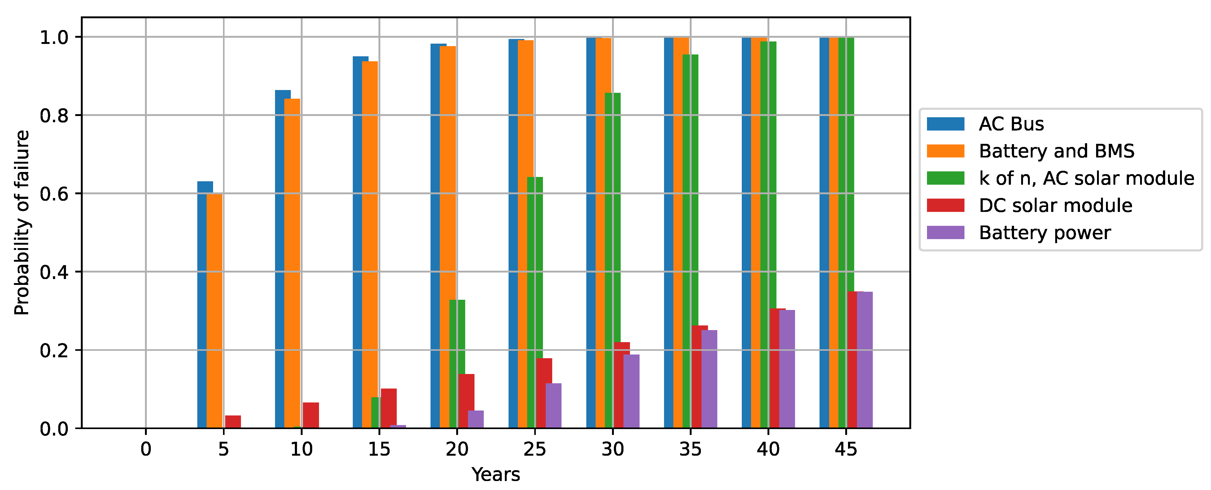
As anticipated, the probability of component failure increases with age. For instance, after 5 years of system operation, the AC bus is expected to have a 63% probability of failure, while the battery and BMS will exhibit a 60.2% probability, and the DC solar module will only have a 3.2% probability of failure. Conversely, for operational periods exceeding 20 years, nearly all system components are likely to experience failure. Specifically, the AC bus is projected to have a 98.2% probability of failure, the battery and BMS a 97.6% probability, and the DC solar module a 13.8% probability of failure.

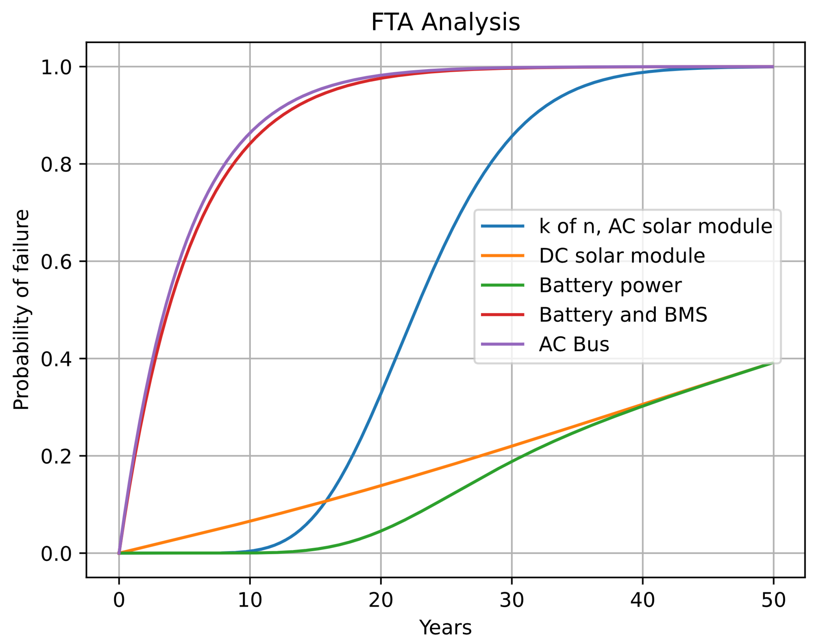
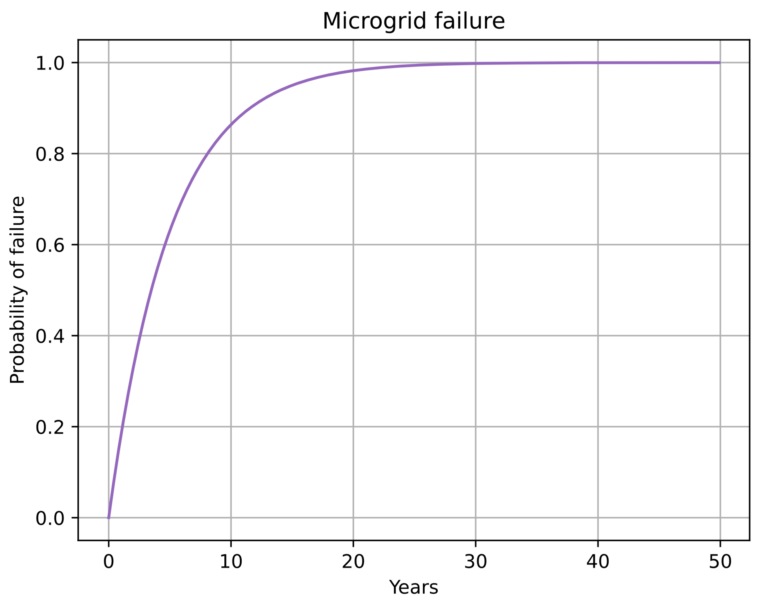
These data are corroborated by Figure 13 and Figure 14. In the former, the failure curves of various sections of the FTA (depicted in Figure 11) are illustrated. Each curve represents intermediate events, with the purple curve signifying the top event related to the total failure of the MG. It is crucial to note that as one delves deeper into the tree, the failure curve undergoes changes. The involvement of a greater number of devices in the analysis corresponds to an increased probability of failure within a shorter time.

Accordingly, Figure 14 provides a clearer depiction of the microgrid’s failure curve, aligning with the failure of the AC bus. This curve closely resembles the failure curve of the battery and the BMS (red curve in Figure 13). Given that the battery and the BMS are the least reliable devices and are in series (represented by an $OR$ gate) with the power failure event, the impact of the battery and BMS predominantly influences the resulting reliability curve. Consequently, the state of the MG is heavily contingent on the status of the battery and BMS. A bar graph illustrating these results is presented in Figure 15.

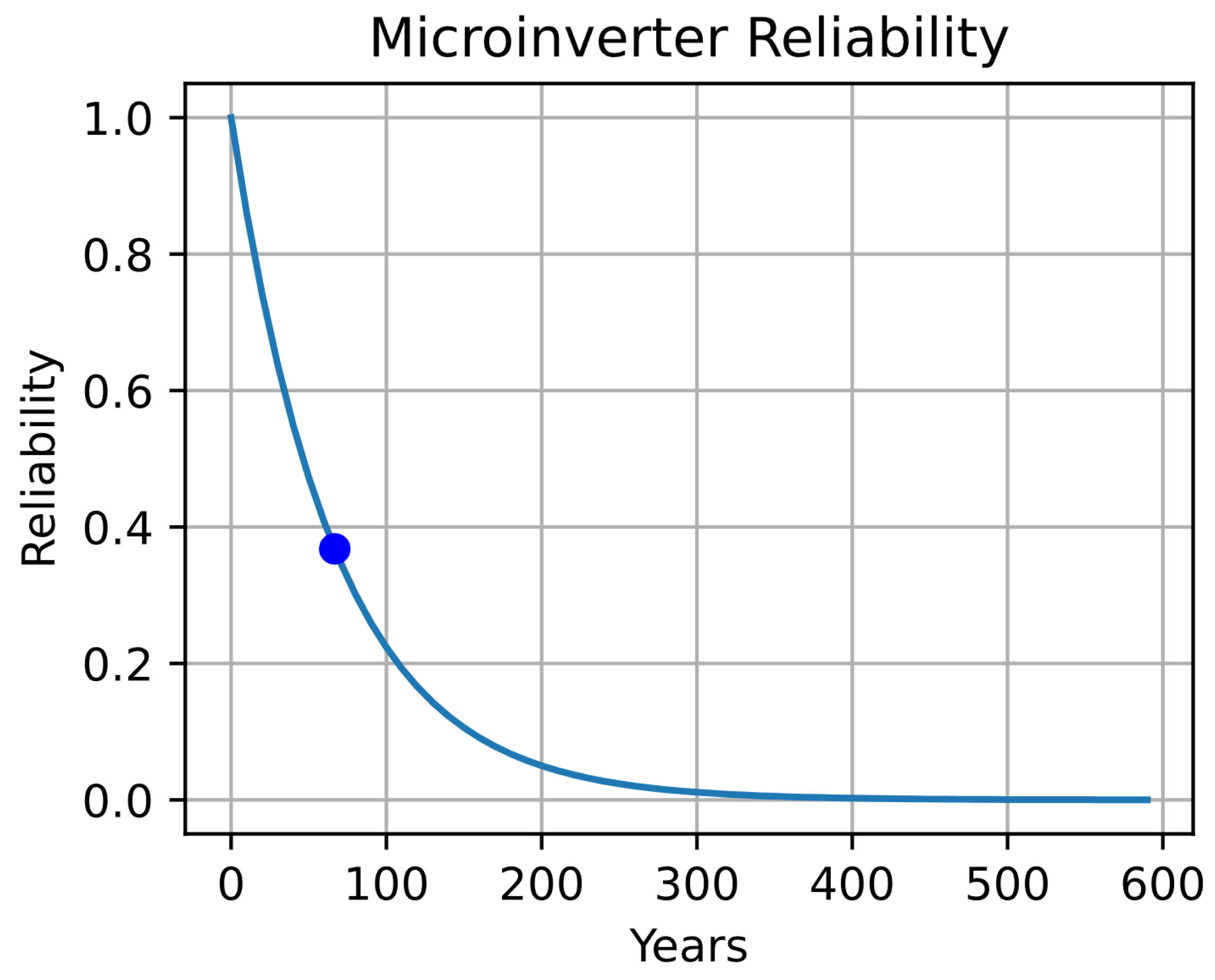
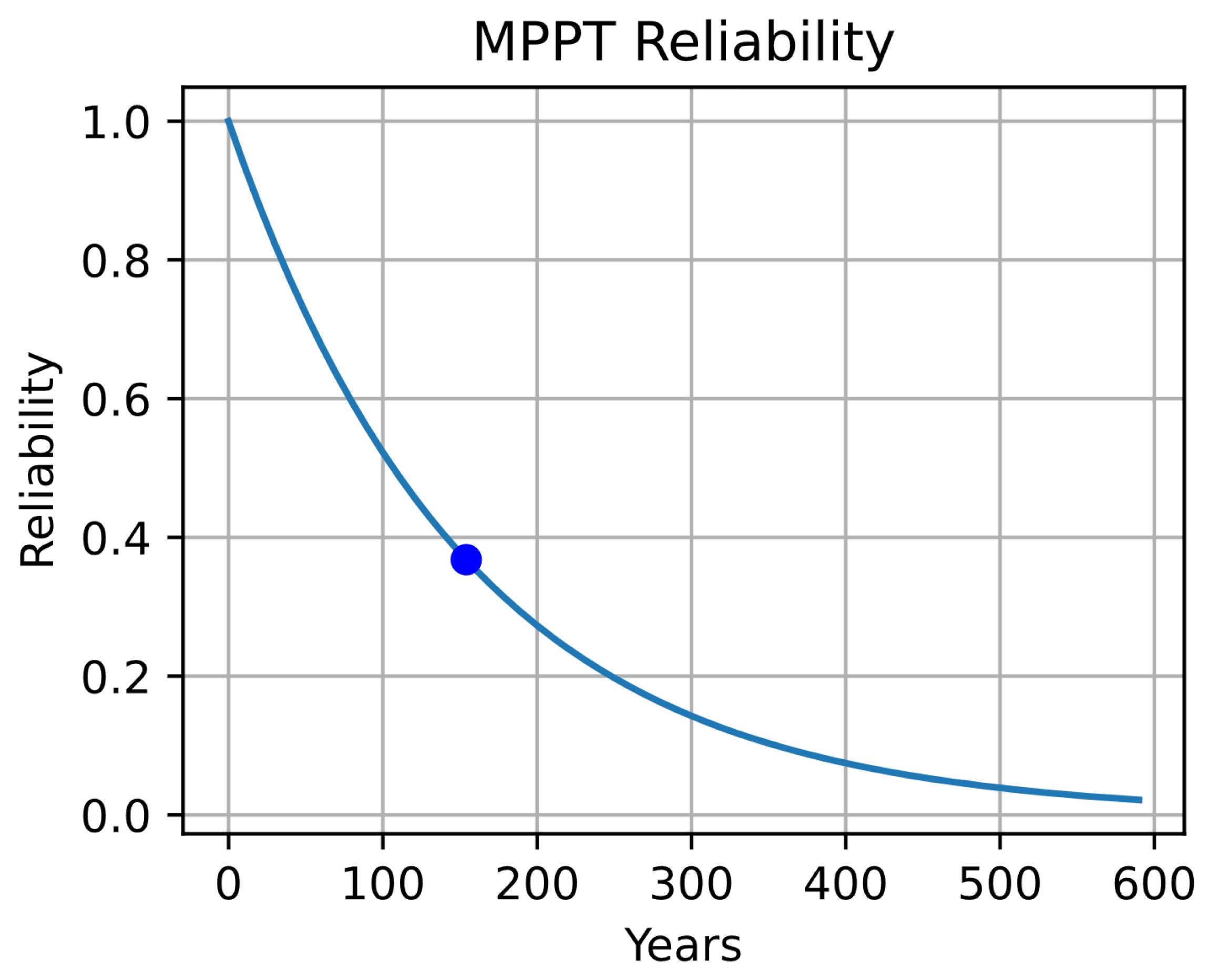
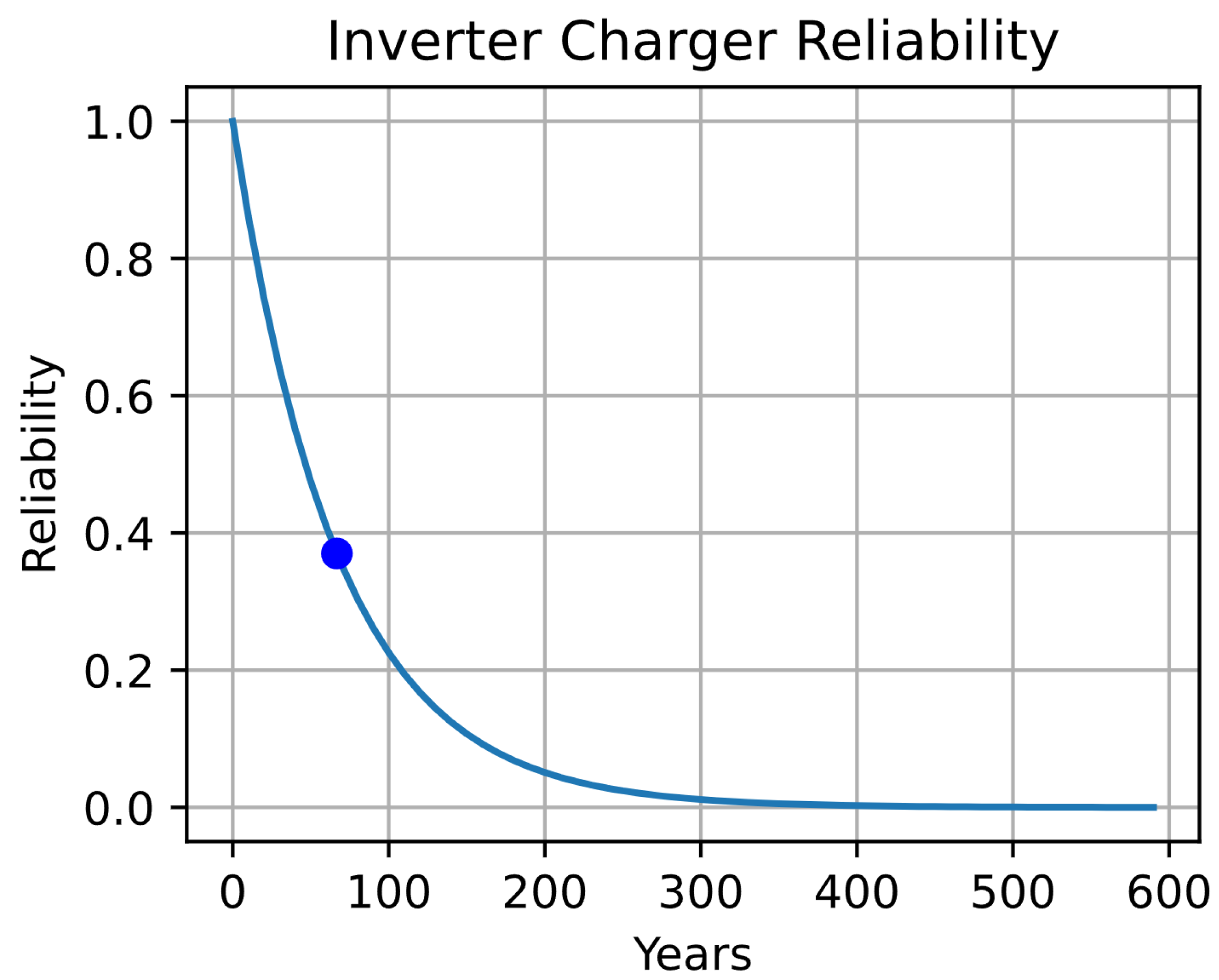
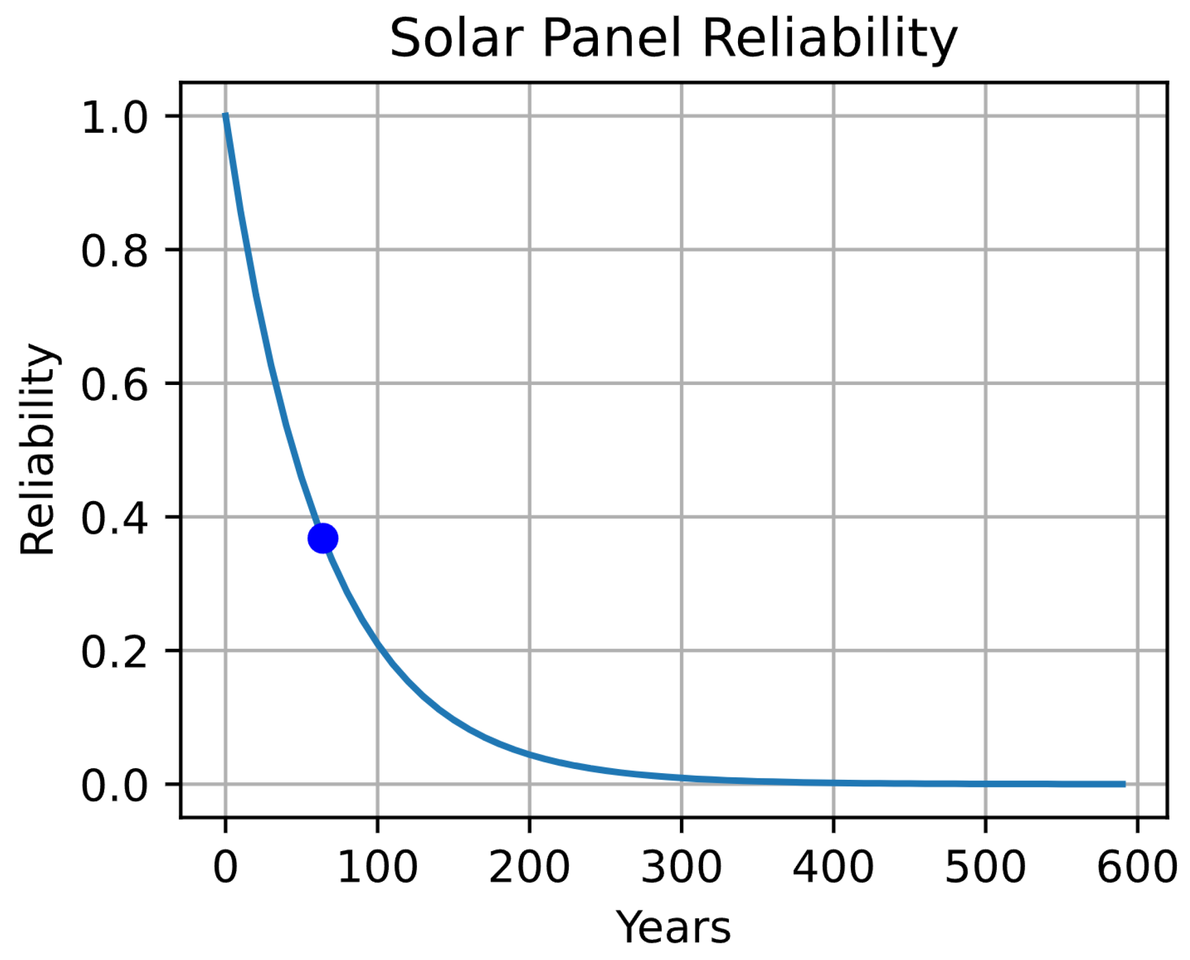
Results of Reliability Analysis

The results presented in Figure 16, Figure 17, Figure 18, Figure 19, Figure 20 and Figure 21 correspond to the reliability curves of the microinverter, Inverter/Charger, MPPT, solar panel, BMS, and battery, respectively.

Although the Fault Tree Analysis is not necessary to obtain the reliability of a single component, the following curves were generated using an algorithm based on the Fiabilipy library [40], in order to compare the individual reliability results with the analysis carried out in our FT model.

The blue dot displayed on each curve represents the MTTF estimated for each device, considering Equation (15) and the failure rates presented in Table 6.

Regarding the reliability of the MPPT (Figure 17), this device exhibits the highest reliability. However, its reliability curve is less steep compared to the others, resulting in a higher MTTF for the MPPT. Conversely, each curve obtained for every device is heavily influenced by the circuit models outlined in Section 2.1. The use of more power elements, capacitors, diodes, and IGBTs in a circuit typically leads to reduced reliability.

In the case of the MPPT, it is the device with a circuit model containing a smaller number of these elements, as depicted in Figure 4. Conversely, the Inverter/Charger exhibits a larger number of capacitors, diodes, and IGBTs, leading to a steeper reliability curve and consequently a lower MTTF value (refer to Figure 3 and Figure 18).

According to these findings, the battery displays the least reliability. This outcome aligns with the data presented in Table 6, where the MTTF of the battery is 8.86 years per failure. Some solar battery manufacturers and distributors suggest that the operational lifespan of a battery is approximately 10 years, depending on its proper operation and size [41]. It is important to note that this lifespan heavily relies on the level of discharge and the discharge cycles provided by each manufacturer for their product.

It is also worth noting that the MTTF values obtained in this study are significantly higher than the reported lifespan provided by manufacturers of MG equipment. Manufacturers tend to be quite conservative when reporting such lifespans in order to avoid creating false expectations among customers.

Results of Importance Measure

The time-based indices of our hybrid MG were calculated over a period of 1000 h of operation and end with an unavailability of 0.023148. Thus, the reliability of this MG is $R\left(t\right)=1-0.023148\approx 97\%$ after 41.67 days of continuous operation. Along with unavailability, several other failure measures are also calculated and presented in

Table 8. Time-based indices for 1000 h.

Time (hrs)	Unavailability	Conditional Failure Intensity	Failure Frequency	Mean Unavailability
0.000	0.000000	23.420000	23.420000	0.000000
100.000	0.002339	23.420000	23.365215	0.001170
200.000	0.004673	23.420000	23.310558	0.002338
300.000	0.007001	23.420001	23.256028	0.003505
400.000	0.009324	23.420001	23.201627	0.004669
500.000	0.011642	23.420002	23.147353	0.005832
600.000	0.013954	23.420002	23.093206	0.006993
700.000	0.016260	23.420003	23.039186	0.008152
800.000	0.018562	23.420004	22.985292	0.009310
900.000	0.020857	23.420006	22.931525	0.010465
1000.000	0.023148	23.420007	22.877883	0.011619

.

Following the timed analysis of the MG, the top three critical components with their failure probabilities are shown in

Table 9. Cut-Sets for 1000 h.

Probability	Events
0.012807	${\mathrm{Battery}}_{\mathrm{Failure}}$
0.008335	${\mathrm{BMS}}_{\mathrm{Failure}}$
0.002158	${\mathrm{Inverter}/\mathrm{Charger}}_{\mathrm{Failure}}$
$2.275956\times {10}^{-9}$	${\mathrm{Microinverter}}_{\mathrm{Failure}}$, ${\mathrm{SolarPanelAC}}_{\mathrm{Failure}}$, ${\mathrm{MPPT}}_{\mathrm{Failure}}$
$1.787111\times {10}^{-14}$	${\mathrm{Microinverter}}_{\mathrm{Failure}}$, ${\mathrm{SolarPanelAC}}_{\mathrm{Failure}}$, ${\mathrm{SolarPanelDC}}_{\mathrm{Failure}}$

for the same period of 1000 h. The basic event whose occurrence would trigger the top event is the failure of the battery with a failure probability of 1.2807%.

Similarly, over a five-year analysis period, time-based indices finish with an unavailability of 0.636477 (refer to

Table 10. Time-based indices for five years.

Time (Years)	Unavailability	Conditional Failure Intensity	Failure Frequency	Mean Unavailability
1 year	0.183191	23.420499	19.130069	0.094682
2 years	0.332829	23.421953	15.626446	0.177607
3 years	0.455063	23.424307	12.764783	0.250406
4 years	0.554912	23.427516	10.427304	0.314472
5 years	0.636477	23.431544	8.517894	0.370991

). Consequently, the reliability of this MG is calculated as $R\left(t\right)=1-0.636477$, yielding approximately 36.35% after five years of uninterrupted operation. Table 10 provides additional failure measures to complement this analysis. Concerning cut-sets, battery failure remains as the basic event whose occurrence would trigger the top event, exhibiting a failure probability of 42.6988%, as illustrated in

Table 11. Cut-Sets for 5 years.

Probability	Events
0.426988	${\mathrm{Battery}}_{\mathrm{Failure}}$
0.303428	${\mathrm{BMS}}_{\mathrm{Failure}}$
0.089091	${\mathrm{Inverter}/\mathrm{Charger}}_{\mathrm{Failure}}$
$1.678368\times {10}^{-4}$	${\mathrm{Microinverter}}_{\mathrm{Failure}}$, ${\mathrm{SolarPanelAC}}_{\mathrm{Failure}}$, ${\mathrm{MPPT}}_{\mathrm{Failure}}$
$2.230790\times {10}^{-6}$	${\mathrm{Microinverter}}_{\mathrm{Failure}}$, ${\mathrm{SolarPanelAC}}_{\mathrm{Failure}}$, ${\mathrm{SolarPanelDC}}_{\mathrm{Failure}}$

. These results are consistent with those presented in Table 7, and Figure 13, Figure 14 and Figure 15 for an operation of five years.

Given Equations (16)–(20), importance measures for the top six critical components of the microgrid were also calculated over five years of operation, and tabulated in

Table 12. Importance Measures of our hybrid MG.

Event	Marginal	Criticality	Diagnostic	Risk Achievement Worth	Risk Reduction Worth
Battery	0.634406	0.425598	0.670861	1.571148	1.740941
BMS	0.521874	0.248793	0.476730	1.571148	1.331191
Inverter/Charger	0.399077	0.055861	0.139975	1.571148	1.059166
Microinverter	$8.679799\times {10}^{-4}$	$9.711004\times {10}^{-5}$	0.071300	1.001267	1.000097
MPPT	0.001936	9.583571 × 10−5	0.031597	1.002946	1.000096
Solar Panel	$1.049981\times {10}^{-5}$	$1.234180\times {10}^{-6}$	0.074815	1.000015	1.000001

.

As noted in the previous results, the three most relevant elements in our microgrid are the battery, the BMS, and the Inverter/Charger, such that the battery presents a marginal importance measure of 63.44%, which represents the contribution that this component will have on the reliability and performance of the entire MG after five years of operation. Conversely, the battery has a criticality measure of 42.55%, referring to the impact on the reliability and performance of the entire microgrid in the event of an eventual failure of this component. Another metric analyzed is the diagnostic importance, in which the battery presents a value of 67.08%, referring to the importance that battery monitoring would have in the ability to eventually detect faults in the complete PV microgrid system.

For its part, the BMS presents a marginal importance measure of 52.18%, a criticality measure of 24.87 %, and a diagnostic measure of 47.67%, which reflects that the BMS would be another component whose permanent monitoring would be important in order to identify possible faults in the microgrid.

Finally, after five years of operation, the Inverter/Charger will present a marginal importance measure of 39.90%, a criticality measure of 5.58%, and a diagnostic measure of 13.99%.

4. Final Discussion

This paper proposes an innovative approach that integrates circuit-level analysis with Probability Density Function selection, reliability function formulation, and Fault Tree Analysis. This methodology delves into the inter-component relationships within microgrids, providing comprehensive insights into system behavior and enabling precise estimations of failure rates. The inclusion of reliability curves and importance measures further aids in identifying potential failures over time, thus facilitating efficient maintenance planning. This aligns with the approach outlined in reference [16], which ensures reliability from the design phase, addressing the inherent challenges posed by power electronics and renewable energy sources. By integrating various system layers, this approach aims to comprehensively build reliability into the microgrid infrastructure.

At the same time, comparing the reliability values and importance measures of our microgrid with those of other studies is challenging due to differences in voltage, power characteristics, and component configurations. However, in [11], a 12 V DC microgrid was examined, featuring two PV arrays equipped with DC-DC boost converters for MPPT, a solar charge controller managing a BESS, and stabilization of boost converter output voltage at 48 $V_{DC}$. Notably, their PV-generating system consisted of two series-connected PV modules with fast-acting DC fuses and a DC circuit breaker. The methodology employed in that study yielded MTTF values of approximately 12.9 years for the PV array, 6.5 years for the boost converter, 15.2 years for the circuit breaker, and around 11.5 years for the overall PV-generating system, such that these findings closely align with the outcomes of our own research.

5. Conclusions

This research introduces an enhanced methodology tailored to address a practical deficit in existing methodologies, integrating circuit-level analysis into the evaluation of building microgrid reliability. By analyzing inter-component relationships, comprehensive insights into system behavior are attained. Leveraging the proposed circuit models and theoretical framework enables precise estimations of microgrid failure rates. Complementing this approach, we propose a thorough investigation utilizing reliability curves and importance measures, offering valuable insights into individual device failure probabilities over time. The application of this methodology to the UdeA Microgrid demonstrates its practical utility and effectiveness.

The integration of circuit-level analysis into microgrid reliability assessment represents a novel approach in the field, addressing a significant gap in existing methodologies. By considering the intricate relationships among components, our methodology offers a more comprehensive understanding of microgrid behavior, paving the way for more accurate reliability assessments.

The insights gained from our methodology hold practical significance for the design, operation, and maintenance of building microgrids. By identifying critical components and their failure probabilities over time, stakeholders can implement proactive maintenance strategies, enhancing microgrid reliability and resilience in real-world applications.

Future research endeavors could focus on refining and validating our methodology across diverse microgrid configurations and operational scenarios. Additionally, advancements in modeling techniques and data analytics could further enhance the accuracy and predictive capabilities of microgrid reliability assessments.

Our findings underscore the importance of proactive maintenance, monitoring, and mitigation strategies in ensuring the long-term reliability and resilience of building microgrid systems. Industry practitioners are encouraged to incorporate circuit-level analysis and time-based reliability assessments into their design and maintenance protocols to optimize microgrid performance and minimize downtime.