
The Explainability of Transformers: Current Status and Directions


Abstract
1. Introduction
- We provide a taxonomy of explainability methods for transformers that relies on the transformer component that the method leverages;
- We describe each method and survey their applications;
- We identify the most favored methods;
- We identify the research gaps and provide some directions for future research.
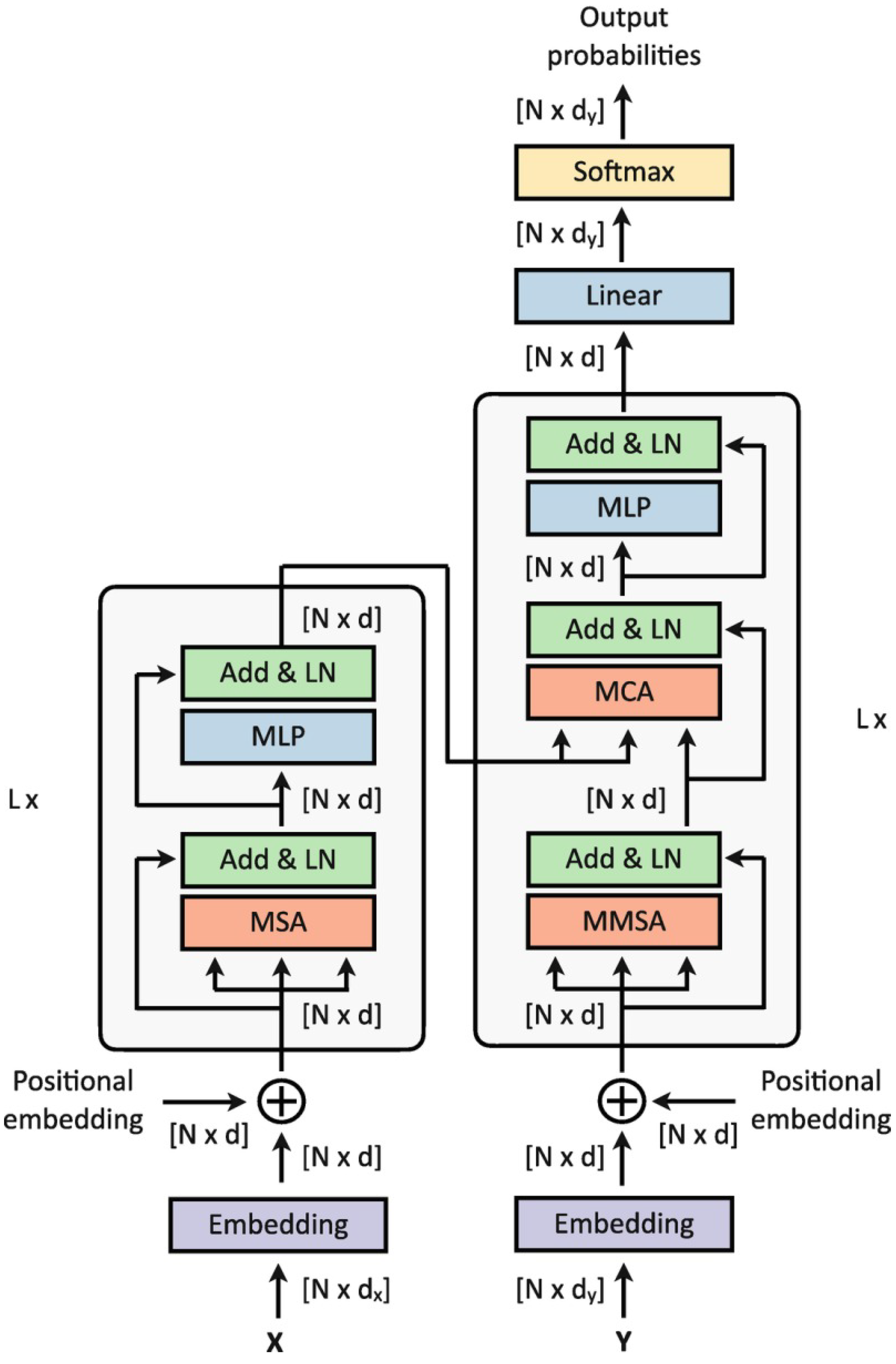
2. Transformers
3. Survey Literature
- Common-attribution methods;
- Attention-based methods;
- Pruning-based methods;
- Inherently explainable methods;
- Non-classification tasks.
- Time coverage;
- Extension, as for the number of papers analyzed;
- Extension, as for the type of application analyzed.
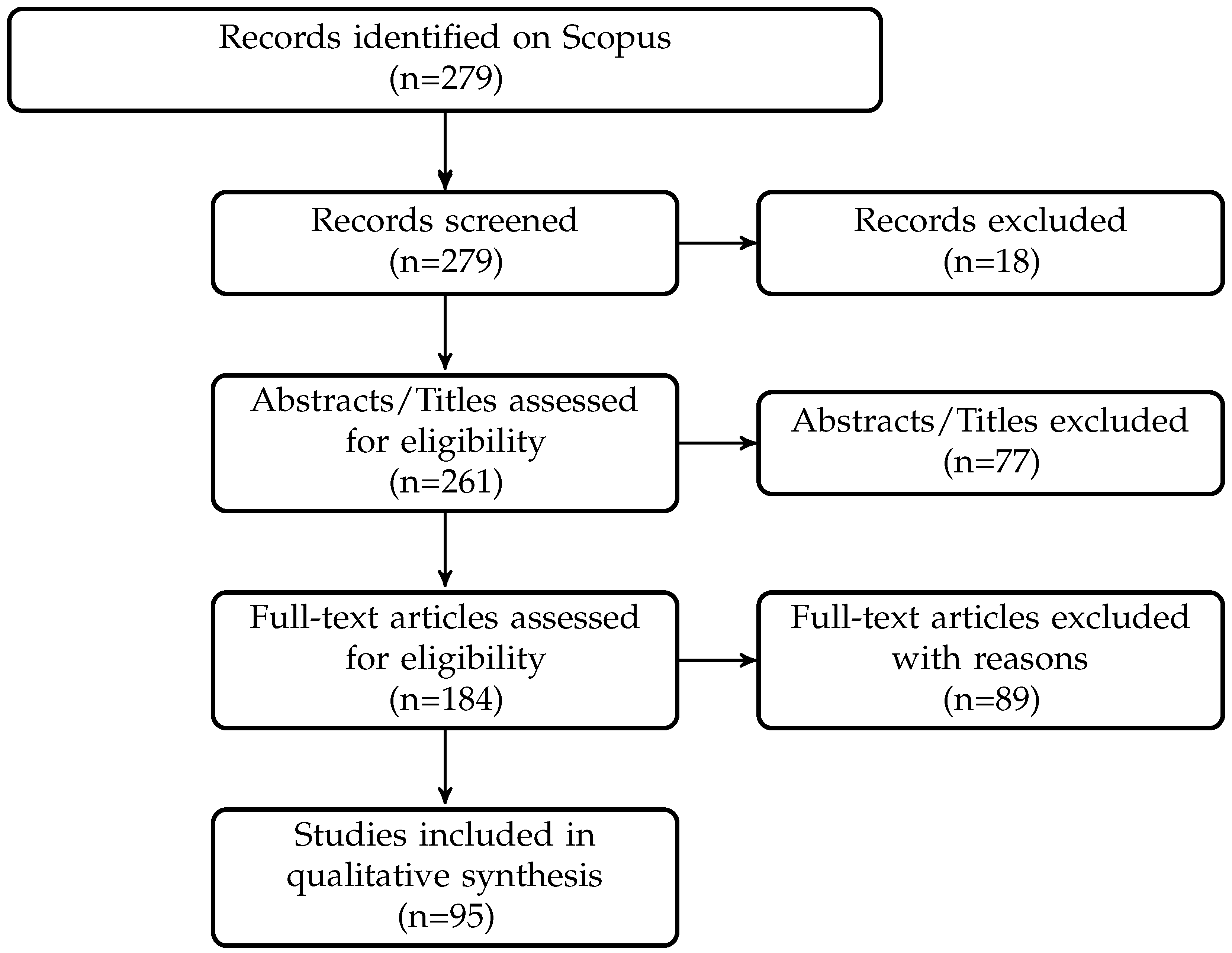
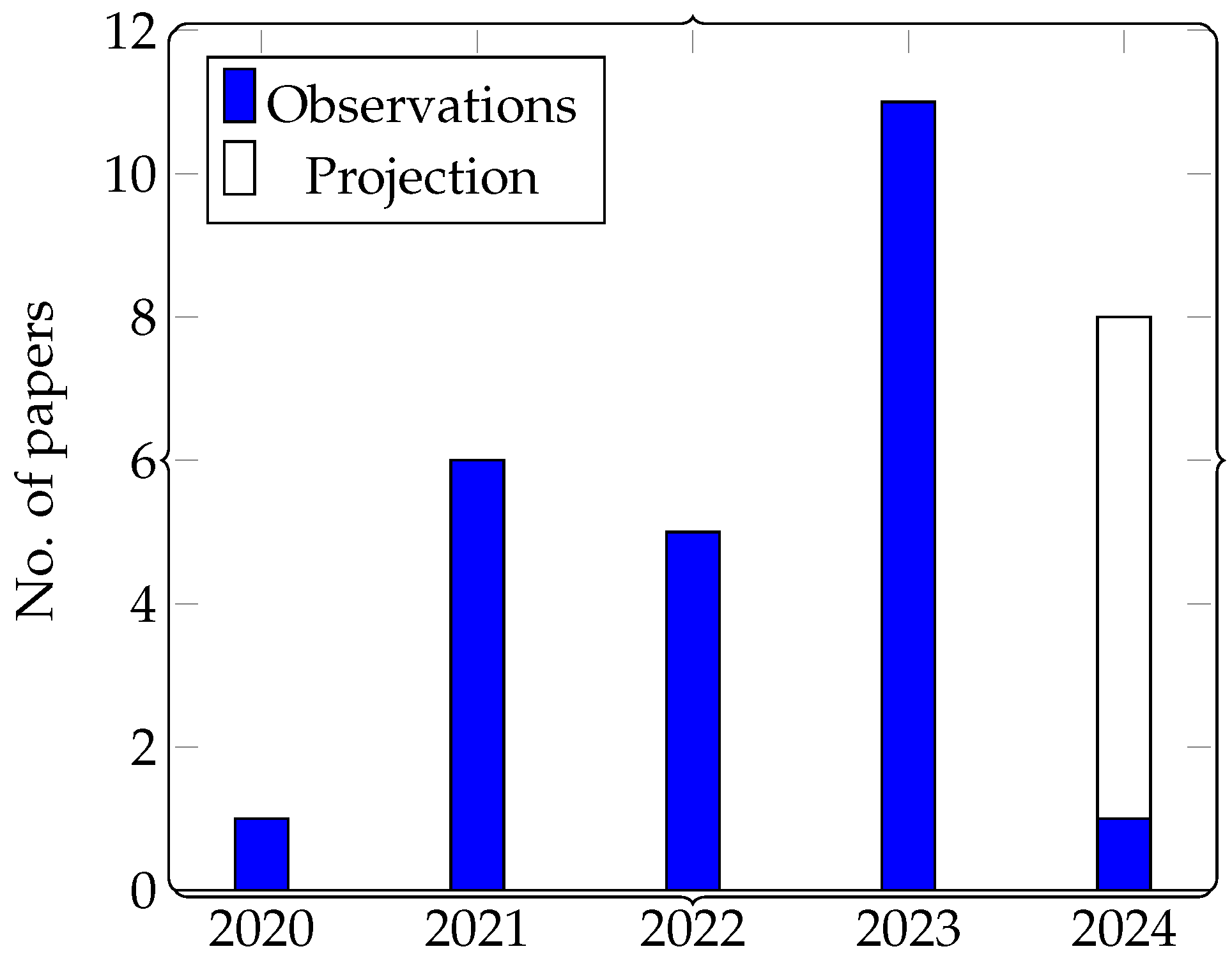
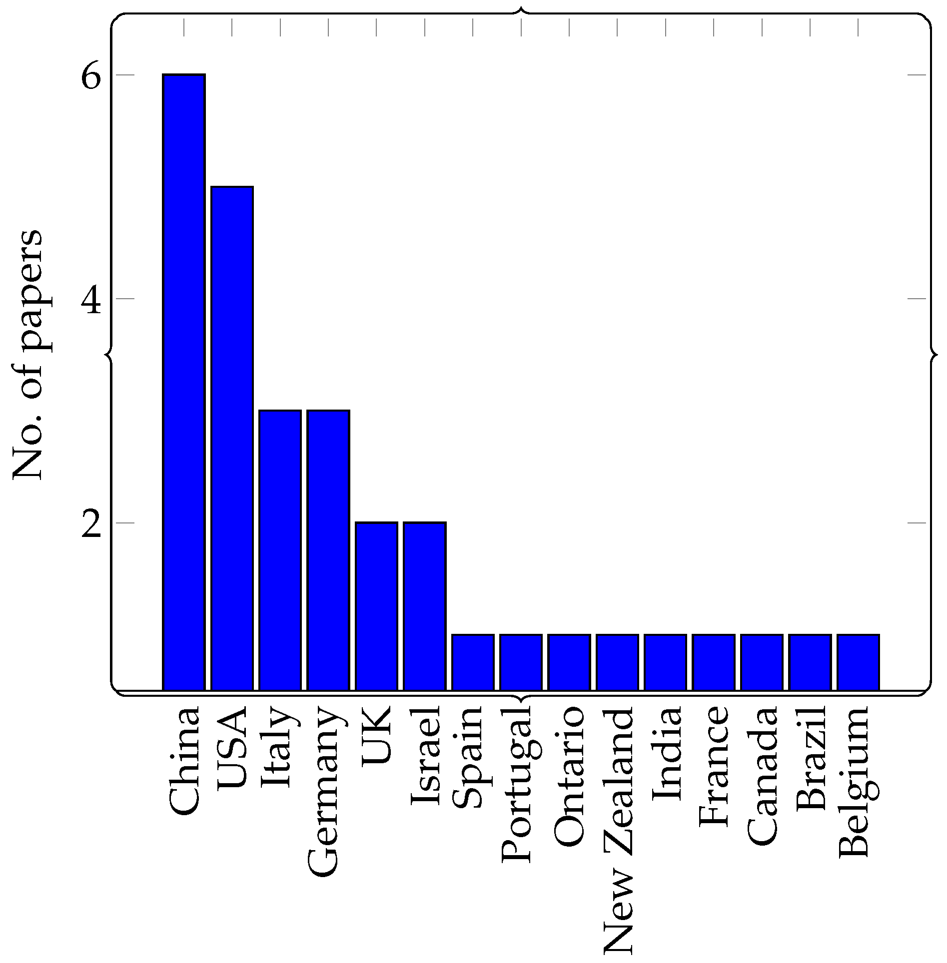
4. Dataset
5. Methodologies for Explainability
- Activation;
- Attention;
- Gradient;
- Perturbation.
5.1. Activation-Based Methods
5.2. Attention-Based Methods
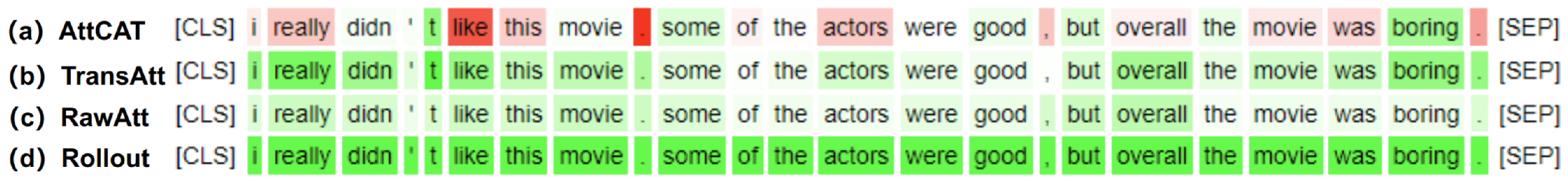
5.3. Gradient-Based Methods
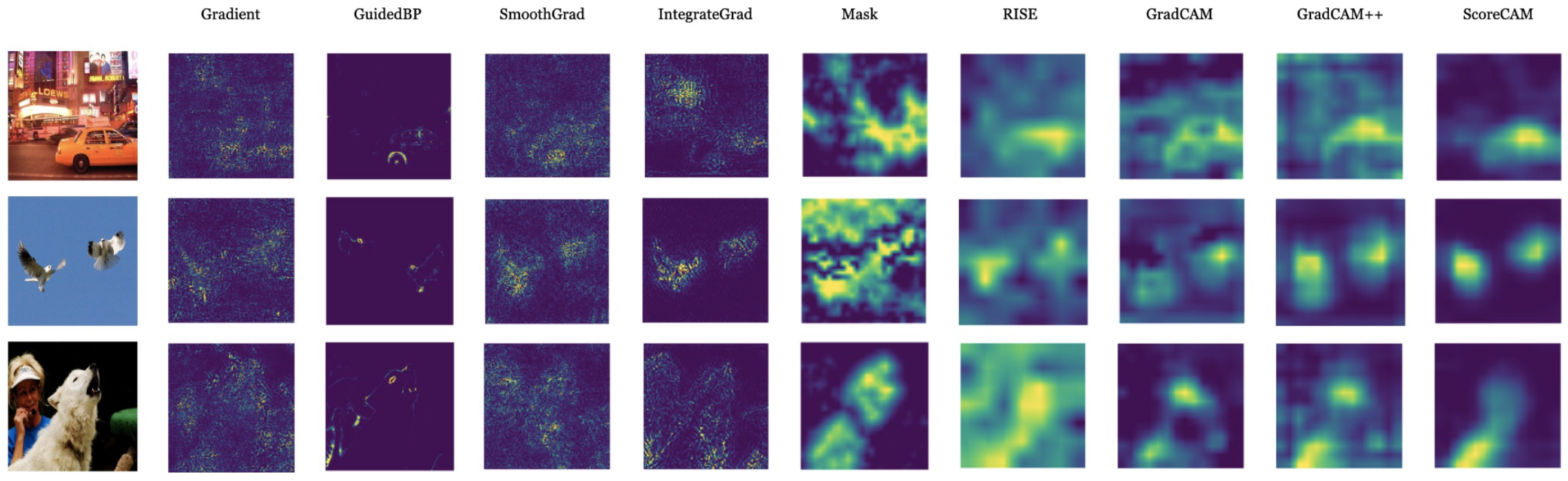
5.4. Perturbation-Based Methods
5.5. Hybrid
5.5.1. Activation + Attention
5.5.2. Activation + Gradient
5.5.3. Activation + Perturbation
5.5.4. Attention + Gradient
5.5.5. Attention + Perturbation
5.5.6. Gradient + Perturbation
5.5.7. Attention + Gradient + Perturbation
5.6. Overall Analysis
6. Discussion and Conclusions
Author Contributions
Funding
Data Availability Statement
Conflicts of Interest
Abbreviations
| AGF | Attribution-Guided Factorization |
| AGrad | Attention Gradient |
| ALTI | Aggregation of Layer-wise Token-to-Token Interactions |
| AttCATs | Attentive Class Activation Tokens |
| BERT | Bidirectional Encoder Representations from Transformers |
| BTs | Bidirectional Transformers |
| Ablation-CAM | Ablation Class Activation Mapping |
| CAM | Class Activation Mapping |
| CAVs | Concept Activation Vectors |
| CLRP | Contrastive Layer-wise Relevance Propagation |
| CLS | Cross-lingual summarization |
| CNN | Convolutional Neural Network |
| DeepLIFT | Deep Learning Important FeaTure |
| DistilBERT | Distilled BERT |
| DeepSHAP | Deep SHapley Additive exPlanations |
| DOAJ | Directory of open-access journals |
| Eigen-CAM | Eigenvalue Class Activation Mapping |
| Grad-CAM | Gradient weighted Class Activation Mapping |
| LIME | Local Interpretable Model-agnostic Explanation |
| LRP | Layer-wise Relevance Propagation |
| LRP-Rollout | Layer-wise Relevance Propagation Rollout |
| MDPI | Multi-disciplinary Digital Publishing Institute |
| ML | Machine Learning |
| NN | Neural network |
| Partial-LRP | Partial Layer-wise Relevance Propagation |
| RAP | Relative Attributing Propagation |
| RePAGrad | Relevance Propagation from Attention Gradient |
| RISE | Randomized Input Sampling for Explanation |
| RoBERTa | Robustly optimized BERT pretraining approach |
| Score-CAM | Score Class Activation Mapping |
| SGLRP | Softmax-Gradient Layer-wise Relevance Propagation |
| SHAP | SHapley Additive exPlanations |
| TAMs | Transition Attention Maps |
| TMME | Transformer Multi-Modal Explainability |
| ViT-CX | Vision Transformers Causal eXplanation |
References
- Islam, S.; Elmekki, H.; Elsebai, A.; Bentahar, J.; Drawel, N.; Rjoub, G.; Pedrycz, W. A comprehensive survey on applications of transformers for deep learning tasks. Expert Syst. Appl. 2023, 241, 122666. [Google Scholar] [CrossRef]
- Parvaiz, A.; Khalid, M.A.; Zafar, R.; Ameer, H.; Ali, M.; Fraz, M.M. Vision Transformers in medical computer vision—A contemplative retrospection. Eng. Appl. Artif. Intell. 2023, 122, 106126. [Google Scholar] [CrossRef]
- Karita, S.; Chen, N.; Hayashi, T.; Hori, T.; Inaguma, H.; Jiang, Z.; Someki, M.; Soplin, N.E.Y.; Yamamoto, R.; Wang, X.; et al. A comparative study on transformer vs rnn in speech applications. In Proceedings of the 2019 IEEE Automatic Speech Recognition and Understanding Workshop (ASRU), Singapore, 14–18 December 2019; pp. 449–456. [Google Scholar]
- Ahmed, S.; Nielsen, I.E.; Tripathi, A.; Siddiqui, S.; Ramachandran, R.P.; Rasool, G. Transformers in time-series analysis: A tutorial. Circuits Syst. Signal Process. 2023, 42, 7433–7466. [Google Scholar] [CrossRef]
- Thampi, A. Interpretable AI: Building Explainable Machine Learning Systems; Simon and Schuster: New York, NY, USA, 2022. [Google Scholar]
- Marcinkevičs, R.; Vogt, J.E. Interpretable and explainable machine learning: A methods-centric overview with concrete examples. WIREs Data Min. Knowl. Discov. 2023, 13, e1493. [Google Scholar] [CrossRef]
- Burkart, N.; Huber, M.F. A survey on the explainability of supervised machine learning. J. Artif. Intell. Res. 2021, 70, 245–317. [Google Scholar] [CrossRef]
- Montavon, G.; Kauffmann, J.; Samek, W.; Müller, K.R. Explaining the predictions of unsupervised learning models. In Proceedings of the International Workshop on Extending Explainable AI Beyond Deep Models and Classifiers, Vienna, Austria, 17 July 2020; Springer: Berlin/Heidelberg, Germany, 2020; pp. 117–138. [Google Scholar]
- Heuillet, A.; Couthouis, F.; Díaz-Rodríguez, N. Explainability in deep reinforcement learning. Knowl.-Based Syst. 2021, 214, 106685. [Google Scholar] [CrossRef]
- Carvalho, D.V.; Pereira, E.M.; Cardoso, J.S. Machine learning interpretability: A survey on methods and metrics. Electronics 2019, 8, 832. [Google Scholar] [CrossRef]
- Van Lent, M.; Fisher, W.; Mancuso, M. An explainable artificial intelligence system for small-unit tactical behavior. In Proceedings of the National Conference on Artificial Intelligence, San Jose, CA, USA, 25–29 July 2004; AAAI Press: Washington, DC, USA, 2004; pp. 900–907. [Google Scholar]
- Bibal, A.; Lognoul, M.; De Streel, A.; Frénay, B. Legal requirements on explainability in machine learning. Artif. Intell. Law 2021, 29, 149–169. [Google Scholar] [CrossRef]
- Waswani, A.; Shazeer, N.; Parmar, N.; Uszkoreit, J.; Jones, L.; Gomez, A.; Kaiser, L.; Polosukhin, I. Attention is all you need. In Advances in Neural Information Processing Systems; Neural Information Processing Systems Foundation, Inc. (NeurIPS): San Diego, CA, USA, 2017. [Google Scholar]
- Vaswani, A.; Shazeer, N.; Parmar, N.; Uszkoreit, J.; Jones, L.; Gomez, A.N.; Kaiser, Ł.; Polosukhin, I. Attention is all you need. Adv. Neural Inf. Process. Syst. 2017, 30, 6000–6010. [Google Scholar]
- Lin, Z.; Feng, M.; Santos, C.N.d.; Yu, M.; Xiang, B.; Zhou, B.; Bengio, Y. A structured self-attentive sentence embedding. In Proceedings of the International Conference on Learning Representations, Toulon, France, 24–26 April 2017. [Google Scholar]
- Bahdanau, D.; Cho, K.; Bengio, Y. Neural Machine Translation by Jointly Learning to Align and Translate. arXiv 2014, arXiv:cs.CL/1409.0473. [Google Scholar]
- Liu, P.J.; Saleh, M.; Pot, E.; Goodrich, B.; Sepassi, R.; Kaiser, L.; Shazeer, N. Generating Wikipedia by Summarizing Long Sequences. In Proceedings of the International Conference on Learning Representations, Vancouver, BC, Canada, 30 April–3 May 2018. [Google Scholar]
- Radford, A.; Narasimhan, K.; Salimans, T.; Sutskever, I. Improving Language Understanding by Generative Pre-Training; Technical Report; OpenAI: San Francisco, CA, USA, 2018. [Google Scholar]
- OpenAI. GPT-4 Technical Report; OpenAI: San Francisco, CA, USA, 2023. [Google Scholar]
- Devlin, J.; Chang, M.W.; Lee, K.; Toutanova, K. BERT: Pre-training of Deep Bidirectional Transformers for Language Understanding. In Proceedings of the 2019 Conference of the North American Chapter of the Association for Computational Linguistics: Human Language Technologies, NAACL-HLT 2019, Minneapolis, MN, USA, 2–7 June 2019; Long and Short Papers. Association for Computational Linguistics: Kerrville, TX, USA, 2019; Volume 1, pp. 4171–4186. [Google Scholar] [CrossRef]
- Liu, Y.; Ott, M.; Goyal, N.; Du, J.; Joshi, M.; Chen, D.; Levy, O.; Lewis, M.; Zettlemoyer, L.; Stoyanov, V. RoBERTa: A robustly optimized BERT pretraining approach. arXiv 2019, arXiv:1907.11692. [Google Scholar]
- Sanh, V.; Debut, L.; Chaumond, J.; Wolf, T. DistilBERT, a distilled version of BERT: Smaller, faster, cheaper and lighter. arXiv 2019, arXiv:1910.01108. [Google Scholar]
- Child, R.; Gray, S.; Radford, A.; Sutskever, I. Generating Long Sequences with Sparse Transformers. arXiv 2019, arXiv:1904.10509. [Google Scholar]
- Katharopoulos, A.; Vyas, A.; Pappas, N.; Fleuret, F. Transformers are RNNs: Fast Autoregressive Transformers with Linear Attention. In Proceedings of the 37th International Conference on Machine Learning, Virtual, 13–18 July 2020. [Google Scholar]
- Guo, Q.; Qiu, X.; Xue, X.; Zhang, Z. Low-Rank and Locality Constrained Self-Attention for Sequence Modeling. IEEE/ACM Trans. Audio Speech Lang. Process. 2019, 27, 2213–2222. [Google Scholar] [CrossRef]
- Li, L.H.; Yatskar, M.; Yin, D.; Hsieh, C.J.; Chang, K.W. VisualBERT: A Simple and Performant Baseline for Vision and Language. arXiv 2019, arXiv:1908.03557. [Google Scholar]
- Alayrac, J.B.; Donahue, J.; Luc, P.; Miech, A.; Barr, I.; Hasson, Y.; Lenc, K.; Mensch, A.; Millican, K.; Reynolds, M.; et al. Flamingo: A visual language model for few-shot learning. Adv. Neural Inf. Process. Syst. 2022, 35, 23716–23736. [Google Scholar]
- Gemini Team, Google. Gemini: A Family of Highly Capable Multimodal Models; Technical Report; Google: Mountain View, CA, USA, 2023. [Google Scholar]
- Colliot, O. Machine Learning for Brain Disorders; Springer Nature: Heidelberg, Germany, 2023. [Google Scholar]
- Zini, J.E.; Awad, M. On the Explainability of Natural Language Processing Deep Models. ACM Comput. Surv. 2022, 55, 1–31. [Google Scholar] [CrossRef]
- Kashefi, R.; Barekatain, L.; Sabokrou, M.; Aghaeipoor, F. Explainability of Vision Transformers: A Comprehensive Review and New Perspectives. arXiv 2023, arXiv:2311.06786. [Google Scholar]
- Vijayakumar, S. Interpretability in Activation Space Analysis of Transformers: A Focused Survey. In Proceedings of the CIKM 2022 Workshops Co-Located with 31st ACM International Conference on Information and Knowledge Management (CIKM 2022), Atlanta, GA, USA, 17–21 October 2022. [Google Scholar]
- Braşoveanu, A.M.P.; Andonie, R. Visualizing Transformers for NLP: A Brief Survey. In Proceedings of the 2020 24th International Conference Information Visualisation (IV), Melbourne, VIC, Australia, 7–11 September 2020; pp. 270–279. [Google Scholar]
- Stassin, S.; Corduant, V.; Mahmoudi, S.A.; Siebert, X. Explainability and Evaluation of Vision Transformers: An In-Depth Experimental Study. Electronics 2023, 13, 175. [Google Scholar] [CrossRef]
- Russakovsky, O.; Deng, J.; Su, H.; Krause, J.; Satheesh, S.; Ma, S.; Huang, Z.; Karpathy, A.; Khosla, A.; Bernstein, M.; et al. Imagenet large scale visual recognition challenge. Int. J. Comput. Vis. 2015, 115, 211–252. [Google Scholar] [CrossRef]
- Page, M.J.; McKenzie, J.E.; Bossuyt, P.M.; Boutron, I.; Hoffmann, T.C.; Mulrow, C.D.; Shamseer, L.; Tetzlaff, J.M.; Akl, E.A.; Brennan, S.E.; et al. The PRISMA 2020 statement: An updated guideline for reporting systematic reviews. Int. J. Surg. 2021, 88, 105906. [Google Scholar] [CrossRef] [PubMed]
- Tricco, A.C.; Lillie, E.; Zarin, W.; O’Brien, K.K.; Colquhoun, H.; Levac, D.; Moher, D.; Peters, M.D.; Horsley, T.; Weeks, L.; et al. PRISMA extension for scoping reviews (PRISMA-ScR): Checklist and explanation. Ann. Intern. Med. 2018, 169, 467–473. [Google Scholar] [CrossRef] [PubMed]
- Bach, S.; Binder, A.; Montavon, G.; Klauschen, F.; Müller, K.R.; Samek, W. On Pixel-Wise Explanations for Non-Linear Classifier Decisions by Layer-Wise Relevance Propagation. PLoS ONE 2015, 10, e0130140. [Google Scholar] [CrossRef] [PubMed]
- Ding, Y.; Liu, Y.; Luan, H.; Sun, M. Visualizing and Understanding Neural Machine Translation. In Proceedings of the 55th Annual Meeting of the Association for Computational Linguistics (Volume 1: Long Papers), Vancouver, BC, Canada, 30 July–4 August 2017; pp. 1150–1159. [Google Scholar]
- Voita, E.; Talbot, D.; Moiseev, F.; Sennrich, R.; Titov, I. Analyzing Multi-Head Self-Attention: Specialized Heads Do the Heavy Lifting, the Rest Can Be Pruned. In Proceedings of the 57th Annual Meeting of the Association for Computational Linguistics, Florence, Italy, 28 July–2 August 2019; pp. 5797–5808. [Google Scholar]
- Chefer, H.; Gur, S.; Wolf, L. Transformer Interpretability Beyond Attention Visualization. In Proceedings of the 2021 IEEE/CVF Conference on Computer Vision and Pattern Recognition (CVPR), Virtual, 19–25 June 2021; pp. 782–791. [Google Scholar]
- Nam, W.J.; Gur, S.; Choi, J.; Wolf, L.; Lee, S.W. Relative Attributing Propagation: Interpreting the Comparative Contributions of Individual Units in Deep Neural Networks. AAAI 2020, 34, 2501–2508. [Google Scholar] [CrossRef]
- Gu, J.; Yang, Y.; Tresp, V. Understanding Individual Decisions of CNNs via Contrastive Backpropagation. In Proceedings of the Computer Vision—ACCV 2018, Perth, Australia, 2–6 December 2018; Springer Nature Switzerland AG: Cham, Switzerland, 2019; pp. 119–134. [Google Scholar]
- Zhou, B.; Khosla, A.; Lapedriza, A.; Oliva, A.; Torralba, A. Learning deep features for discriminative localization. In Proceedings of the 2016 IEEE Conference on Computer Vision and Pattern Recognition (CVPR), Las Vegas, NV, USA, 27–30 June 2016. [Google Scholar]
- Ferrando, J.; Gállego, G.I.; Costa-jussà, M.R. Measuring the Mixing of Contextual Information in the Transformer. In Proceedings of the 2022 Conference on Empirical Methods in Natural Language Processing, Abu Dhabi, United Arab Emirates, 7–11 December 2022; pp. 8698–8714. [Google Scholar]
- Li, J.; Monroe, W.; Jurafsky, D. Understanding Neural Networks through Representation Erasure. arXiv 2016, arXiv:1612.08220. [Google Scholar]
- Kim, B.; Wattenberg, M.; Gilmer, J.; Cai, C.; Wexler, J.; Viegas, F.; Sayres, R. Interpretability Beyond Feature Attribution: Quantitative Testing with Concept Activation Vectors (TCAV). In Proceedings of the 35th International Conference on Machine Learning, Stockholm, Sweden, 10–15 July 2018; Volume 80, pp. 2668–2677. [Google Scholar]
- Muhammad, M.B.; Yeasin, M. Eigen-CAM: Class Activation Map using Principal Components. In Proceedings of the 2020 International Joint Conference on Neural Networks (IJCNN), Glasgow, UK, 19–24 July 2020; pp. 1–7. [Google Scholar]
- Mishra, R.; Yadav, A.; Shah, R.R.; Kumaraguru, P. Explaining Finetuned Transformers on Hate Speech Predictions Using Layerwise Relevance Propagation. In Proceedings of the Big Data and Artificial Intelligence, Delhi, India, 7–9 December 2023; Springer Nature: Cham, Switzerland, 2023; pp. 201–214. [Google Scholar]
- Thorn Jakobsen, T.S.; Cabello, L.; Søgaard, A. Being Right for Whose Right Reasons? In Proceedings of the 61st Annual Meeting of the Association for Computational Linguistics (Volume 1: Long Papers), Toronto, ON, Canada, 9–14 July 2023; pp. 1033–1054. [Google Scholar]
- Yu, L.; Xiang, W. X-Pruner: eXplainable Pruning for Vision Transformers. In Proceedings of the 2023 IEEE/CVF Conference on Computer Vision and Pattern Recognition (CVPR), Vancouver, BC, Canada, 18–22 June 2023; pp. 24355–24363. [Google Scholar]
- Chan, A.; Schneider, M.; Körner, M. XAI for Early Crop Classification. In Proceedings of the 2023 IEEE International Geoscience and Remote Sensing Symposium (IGARSS), Pasadena, CA, USA, 16–21 July 2023; pp. 2657–2660. [Google Scholar]
- Yang, Y.; Jiao, L.; Liu, F.; Liu, X.; Li, L.; Chen, P.; Yang, S. An Explainable Spatial–Frequency Multiscale Transformer for Remote Sensing Scene Classification. IEEE Trans. Geosci. Remote Sens. 2023, 61, 1–15. [Google Scholar] [CrossRef]
- Ferrando, J.; Gállego, G.I.; Tsiamas, I.; Costa-Jussà, M.R. Explaining How Transformers Use Context to Build Predictions. In Proceedings of the 61st Annual Meeting of the Association for Computational Linguistics, Toronto, ON, Canada, 9–14 July 2023; Volume 1: Long Papersm, pp. 5486–5513. [Google Scholar]
- Madsen, A.G.; Lehn-Schioler, W.T.; Jonsdottir, A.; Arnardottir, B.; Hansen, L.K. Concept-Based Explainability for an EEG Transformer Model. In Proceedings of the 2023 IEEE 33rd International Workshop on Machine Learning for Signal Processing (MLSP), Rome, Italy, 17–20 September 2023; pp. 1–6. [Google Scholar]
- Ramesh, K.; Koh, Y.S. Investigation of Explainability Techniques for Multimodal Transformers. In Communications in Computer and Information Science; Communications in Computer and Information Science; Springer Nature: Singapore, 2022; pp. 90–98. [Google Scholar]
- Hroub, N.A.; Alsannaa, A.N.; Alowaifeer, M.; Alfarraj, M.; Okafor, E. Explainable deep learning diagnostic system for prediction of lung disease from medical images. Comput. Biol. Med. 2024, 170, 108012. [Google Scholar] [CrossRef] [PubMed]
- Alammar, J. Ecco: An Open Source Library for the Explainability of Transformer Language Models. In Proceedings of the 59th Annual Meeting of the Association for Computational Linguistics and the 11th International Joint Conference on Natural Language Processing: System Demonstrations, Online, 1–6 August 2021; pp. 249–257. [Google Scholar]
- van Aken, B.; Winter, B.; Löser, A.; Gers, F.A. VisBERT: Hidden-State Visualizations for Transformers. In Proceedings of the Web Conference 2020, Taipei, Taiwan, 20–24 April 2020; pp. 207–211. [Google Scholar]
- Gao, Y.; Wang, P.; Zeng, X.; Chen, L.; Mao, Y.; Wei, Z.; Li, M. Towards Explainable Table Interpretation Using Multi-view Explanations. In Proceedings of the 2023 IEEE 39th International Conference on Data Engineering (ICDE), Anaheim, CA, USA, 3–7 April 2023; pp. 1167–1179. [Google Scholar]
- Abnar, S.; Zuidema, W. Quantifying Attention Flow in Transformers. In Proceedings of the 58th Annual Meeting of the Association for Computational Linguistics, Online, 5–10 July 2020; pp. 4190–4197. [Google Scholar]
- Renz, K.; Chitta, K.; Mercea, O.B.; Koepke, A.S.; Akata, Z.; Geiger, A. PlanT: Explainable Planning Transformers via Object-Level Representations. In Proceedings of the 6th Conference on Robot Learning, Auckland, New Zealand, 14–18 December 2022; Volume 205, pp. 459–470. [Google Scholar]
- Feng, Q.; Yuan, J.; Emdad, F.B.; Hanna, K.; Hu, X.; He, Z. Can Attention Be Used to Explain EHR-Based Mortality Prediction Tasks: A Case Study on Hemorrhagic Stroke. In Proceedings of the 14th ACM International Conference on Bioinformatics, Computational Biology, and Health Informatics, Houston TX USA, 3–6 September 2023; pp. 1–6. [Google Scholar]
- Trisedya, B.D.; Salim, F.D.; Chan, J.; Spina, D.; Scholer, F.; Sanderson, M. i-Align: An interpretable knowledge graph alignment model. Data Min. Knowl. Discov. 2023, 37, 2494–2516. [Google Scholar] [CrossRef]
- Graca, M.; Marques, D.; Santander-Jiménez, S.; Sousa, L.; Ilic, A. Interpreting High Order Epistasis Using Sparse Transformers. In Proceedings of the 8th ACM/IEEE International Conference on Connected Health: Applications, Systems and Engineering Technologies, Orlando, FL, USA, 21–23 June 2023; pp. 114–125. [Google Scholar]
- Kim, B.H.; Deng, Z.; Yu, P.; Ganapathi, V. Can Current Explainability Help Provide References in Clinical Notes to Support Humans Annotate Medical Codes? In Proceedings of the 13th International Workshop on Health Text Mining and Information Analysis (LOUHI), Abu Dhabi, United Arab Emirates, 7 December 2022; pp. 26–34. [Google Scholar]
- Clauwaert, J.; Menschaert, G.; Waegeman, W. Explainability in transformer models for functional genomics. Brief. Bioinform. 2021, 22, bbab060. [Google Scholar] [CrossRef]
- Sebbaq, H.; El Faddouli, N.E. MTBERT-Attention: An Explainable BERT Model based on Multi-Task Learning for Cognitive Text Classification. Sci. Afr. 2023, 21, e01799. [Google Scholar] [CrossRef]
- Chen, H.; Zhou, K.; Jiang, Z.; Yeh, C.C.M.; Li, X.; Pan, M.; Zheng, Y.; Hu, X.; Yang, H. Probabilistic masked attention networks for explainable sequential recommendation. In Proceedings of the Thirty-Second International Joint Conference on Artificial Intelligence, Macao, China, 19–25 August 2023. [Google Scholar]
- Wantiez, A.; Qiu, T.; Matthes, S.; Shen, H. Scene Understanding for Autonomous Driving Using Visual Question Answering. In Proceedings of the 2023 International Joint Conference on Neural Networks (IJCNN), Gold Coast, Australia, 18–22 June 2023; pp. 1–7. [Google Scholar]
- Ou, L.; Chang, Y.C.; Wang, Y.K.; Lin, C.T. Fuzzy Centered Explainable Network for Reinforcement Learning. IEEE Trans. Fuzzy Syst. 2024, 32, 203–213. [Google Scholar] [CrossRef]
- Schwenke, L.; Atzmueller, M. Show me what you’re looking for. Int. Flairs Conf. Proc. 2021, 34, 128399. [Google Scholar] [CrossRef]
- Schwenke, L.; Atzmueller, M. Constructing Global Coherence Representations: Identifying Interpretability and Coherences of Transformer Attention in Time Series Data. In Proceedings of the 2021 IEEE 8th International Conference on Data Science and Advanced Analytics (DSAA), Porto, Portugal, 6–9 October 2021; pp. 1–12. [Google Scholar]
- Bacco, L.; Cimino, A.; Dell’Orletta, F.; Merone, M. Extractive Summarization for Explainable Sentiment Analysis using Transformers. In Proceedings of the Sixth International Workshop on eXplainable SENTIment Mining and EmotioN deTection, Hersonissos, Greece, 7 June 2021. [Google Scholar]
- Bacco, L.; Cimino, A.; Dell’Orletta, F.; Merone, M. Explainable Sentiment Analysis: A Hierarchical Transformer-Based Extractive Summarization Approach. Electronics 2021, 10, 2195. [Google Scholar] [CrossRef]
- Humphreys, J.; Dam, H.K. An Explainable Deep Model for Defect Prediction. In Proceedings of the 2019 IEEE/ACM 7th International Workshop on Realizing Artificial Intelligence Synergies in Software Engineering (RAISE), Montreal, QC, Canada, 28 May 2019; pp. 49–55. [Google Scholar]
- Hickmann, M.L.; Wurzberger, F.; Hoxhalli, M.; Lochner, A.; Töllich, J.; Scherp, A. Analysis of GraphSum’s Attention Weights to Improve the Explainability of Multi-Document Summarization. In Proceedings of the The 23rd International Conference on Information Integration and Web Intelligence, Linz, Austria, 29 November–1 December 2021; pp. 359–366. [Google Scholar]
- Di Nardo, E.; Ciaramella, A. Tracking vision transformer with class and regression tokens. Inf. Sci. 2023, 619, 276–287. [Google Scholar] [CrossRef]
- Cremer, J.; Medrano Sandonas, L.; Tkatchenko, A.; Clevert, D.A.; De Fabritiis, G. Equivariant Graph Neural Networks for Toxicity Prediction. Chem. Res. Toxicol. 2023, 36, 1561–1573. [Google Scholar] [CrossRef] [PubMed]
- Pasquadibisceglie, V.; Appice, A.; Castellano, G.; Malerba, D. JARVIS: Joining Adversarial Training with Vision Transformers in Next-Activity Prediction. IEEE Trans. Serv. Comput. 2023, 01, 1–14. [Google Scholar] [CrossRef]
- Neto, A.; Ferreira, S.; Libânio, D.; Dinis-Ribeiro, M.; Coimbra, M.; Cunha, A. Preliminary study of deep learning algorithms for metaplasia detection in upper gastrointestinal endoscopy. In Proceedings of the International Conference on Wireless Mobile Communication and Healthcare, Virtual Event, 30 November–2 December 2022; Springer Nature: Cham, Switzerland, 2023; pp. 34–50. [Google Scholar]
- Komorowski, P.; Baniecki, H.; Biecek, P. Towards evaluating explanations of vision transformers for medical imaging. In Proceedings of the 2023 IEEE/CVF Conference on Computer Vision and Pattern Recognition Workshops (CVPRW), Vancouver, BC, Canada, 18–22 June 2023; pp. 3726–3732. [Google Scholar]
- Fiok, K.; Karwowski, W.; Gutierrez, E.; Wilamowski, M. Analysis of sentiment in tweets addressed to a single domain-specific Twitter account: Comparison of model performance and explainability of predictions. Expert Syst. Appl. 2021, 186, 115771. [Google Scholar] [CrossRef]
- Tagarelli, A.; Simeri, A. Unsupervised law article mining based on deep pre-trained language representation models with application to the Italian civil code. Artif. Intell. Law 2022, 30, 417–473. [Google Scholar] [CrossRef]
- Lal, V.; Ma, A.; Aflalo, E.; Howard, P.; Simoes, A.; Korat, D.; Pereg, O.; Singer, G.; Wasserblat, M. InterpreT: An Interactive Visualization Tool for Interpreting Transformers. In Proceedings of the 16th Conference of the European Chapter of the Association for Computational Linguistics: System Demonstrations, Online, 19–23 April 2021; pp. 135–142. [Google Scholar]
- Dai, Y.; Jayaratne, M.; Jayatilleke, B. Explainable Personality Prediction Using Answers to Open-Ended Interview Questions. Front. Psychol. 2022, 13, 865841. [Google Scholar] [CrossRef] [PubMed]
- Gaiger, K.; Barkan, O.; Tsipory-Samuel, S.; Koenigstein, N. Not All Memories Created Equal: Dynamic User Representations for Collaborative Filtering. IEEE Access 2023, 11, 34746–34763. [Google Scholar] [CrossRef]
- Zeng, W.; Gautam, A.; Huson, D.H. MuLan-Methyl-multiple transformer-based language models for accurate DNA methylation prediction. Gigascience 2022, 12, giad054. [Google Scholar] [CrossRef] [PubMed]
- Belainine, B.; Sadat, F.; Boukadoum, M. End-to-End Dialogue Generation Using a Single Encoder and a Decoder Cascade With a Multidimension Attention Mechanism. IEEE Trans. Neural Netw. Learn. Syst. 2023, 34, 8482–8492. [Google Scholar] [CrossRef] [PubMed]
- Ye, X.; Xiao, M.; Ning, Z.; Dai, W.; Cui, W.; Du, Y.; Zhou, Y. NEEDED: Introducing Hierarchical Transformer to Eye Diseases Diagnosis. In Proceedings of the 2023 SIAM International Conference on Data Mining (SDM), Minneapolis-St. Paul Twin Cities, MN, USA, 27–29 April 2023; pp. 667–675. [Google Scholar]
- Kan, X.; Gu, A.A.C.; Cui, H.; Guo, Y.; Yang, C. Dynamic Brain Transformer with Multi-Level Attention for Functional Brain Network Analysis. In Proceedings of the 2023 IEEE EMBS International Conference on Biomedical and Health Informatics (BHI), Pittsburgh, PA, USA, 15–18 October 2023; pp. 1–4. [Google Scholar]
- Qu, G.; Orlichenko, A.; Wang, J.; Zhang, G.; Xiao, L.; Zhang, K.; Wilson, T.W.; Stephen, J.M.; Calhoun, V.D.; Wang, Y.P. Interpretable Cognitive Ability Prediction: A Comprehensive Gated Graph Transformer Framework for Analyzing Functional Brain Networks. IEEE Trans. Med. Imaging 2023, 43, 1568–1578. [Google Scholar] [CrossRef] [PubMed]
- Sonth, A.; Sarkar, A.; Bhagat, H.; Abbott, L. Explainable Driver Activity Recognition Using Video Transformer in Highly Automated Vehicle. In Proceedings of the 2023 IEEE Intelligent Vehicles Symposium (IV), Anchorage, AK, USA, 4–7 June 2023; pp. 1–8. [Google Scholar]
- Shih, J.-L.; Kashihara, A.; Chen, W.; Chen, W.; Ogata, H.; Baker, R.; Chang, B.; Dianati, S.; Madathil, J.; Yousef, A.M.F.; et al. (Eds.) Recommending Learning Actions Using Neural Network. In Proceedings of the 31st International Conference on Computers in Education, Matsue, Japan, 4–8 December 2023. [Google Scholar]
- Wang, L.; Huang, J.; Xing, X.; Yang, G. Hybrid Swin Deformable Attention U-Net for Medical Image Segmentation; Institute of Electrical and Electronics Engineers Inc.: Piscataway, NJ, USA, 2023. [Google Scholar]
- Kim, J.; Kim, T.; Kim, J. Two-pathway spatiotemporal representation learning for extreme water temperature prediction. Eng. Appl. Artif. Intell. 2024, 131, 107718. [Google Scholar] [CrossRef]
- Monteiro, N.R.C.; Oliveira, J.L.; Arrais, J.P. TAG-DTA: Binding-region-guided strategy to predict drug-target affinity using transformers. Expert Syst. Appl. 2024, 238, 122334. [Google Scholar] [CrossRef]
- Yadav, S.; Kaushik, A.; McDaid, K. Understanding Interpretability: Explainable AI Approaches for Hate Speech Classifiers. In Explainable Artificial Intelligence; Springer Nature: Cham, Switzerland, 2023; pp. 47–70. [Google Scholar]
- Ma, J.; Bai, Y.; Zhong, B.; Zhang, W.; Yao, T.; Mei, T. Visualizing and Understanding Patch Interactions in Vision Transformer. IEEE Trans. Neural Netw. Learn. Syst. 2023. [Google Scholar] [CrossRef] [PubMed]
- Simonyan, K.; Vedaldi, A.; Zisserman, A. Deep Inside Convolutional Networks: Visualising Image Classification Models and Saliency Maps. In Proceedings of the Workshop at International Conference on Learning Representations, Banff, AB, Canada, 14–16 April 2014. [Google Scholar]
- Springenberg, J.T.; Dosovitskiy, A.; Brox, T.; Riedmiller, M. Striving for Simplicity: The All Convolutional Net. In Proceedings of the 3rd International Conference on Learning Representations, ICLR 2015, San Diego, CA, USA, 7–9 May 2015; Workshop Track Proceedings. Bengio, Y., LeCun, Y., Eds.; 2015. [Google Scholar]
- Kindermans, P.J.; Schütt, K.; Müller, K.R.; Dähne, S. Investigating the influence of noise and distractors on the interpretation of neural networks. arXiv 2016, arXiv:1611.07270. [Google Scholar]
- Yin, K.; Neubig, G. Interpreting Language Models with Contrastive Explanations. In Proceedings of the 2022 Conference on Empirical Methods in Natural Language Processing, Abu Dhabi, United Arab Emirates, 7–11 December 2022; pp. 184–198. [Google Scholar]
- Selvaraju, R.R.; Cogswell, M.; Das, A.; Vedantam, R.; Parikh, D.; Batra, D. Grad-CAM: Visual explanations from deep networks via Gradient-based localization. In Proceedings of the 2017 IEEE International Conference on Computer Vision (ICCV), Venice, Italy, 22–29 October 2017; pp. 618–626. [Google Scholar] [CrossRef]
- Chattopadhay, A.; Sarkar, A.; Howlader, P.; Balasubramanian, V.N. Grad-CAM++: Generalized Gradient-Based Visual Explanations for Deep Convolutional Networks. In Proceedings of the 2018 IEEE Winter Conference on Applications of Computer Vision (WACV), Lake Tahoe, NV, USA, 12–15 March 2018; pp. 839–847. [Google Scholar]
- Sobahi, N.; Atila, O.; Deniz, E.; Sengur, A.; Acharya, U.R. Explainable COVID-19 detection using fractal dimension and vision transformer with Grad-CAM on cough sounds. Biocybern. Biomed. Eng. 2022, 42, 1066–1080. [Google Scholar] [CrossRef] [PubMed]
- Thon, P.L.; Than, J.C.M.; Kassim, R.M.; Yunus, A.; Noor, N.M.; Then, P. Explainable COVID-19 Three Classes Severity Classification Using Chest X-Ray Images. In Proceedings of the 2022 IEEE-EMBS Conference on Biomedical Engineering and Sciences (IECBES), Kuala Lumpur, Malaysia, 7–9 December 2022; pp. 312–317. [Google Scholar]
- Vaid, A.; Jiang, J.; Sawant, A.; Lerakis, S.; Argulian, E.; Ahuja, Y.; Lampert, J.; Charney, A.; Greenspan, H.; Narula, J.; et al. A foundational vision transformer improves diagnostic performance for electrocardiograms. NPJ Digit. Med. 2023, 6, 108. [Google Scholar] [CrossRef] [PubMed]
- Wang, J.; Qu, A.; Wang, Q.; Zhao, Q.; Liu, J.; Wu, Q. TT-Net: Tensorized Transformer Network for 3D medical image segmentation. Comput. Med. Imaging Graph. 2023, 107, 102234. [Google Scholar] [CrossRef] [PubMed]
- Wollek, A.; Graf, R.; Čečatka, S.; Fink, N.; Willem, T.; Sabel, B.O.; Lasser, T. Attention-based Saliency Maps Improve Interpretability of Pneumothorax Classification. Radiol. Artif. Intell. 2023, 5, e220187. [Google Scholar] [CrossRef] [PubMed]
- Thakur, P.S.; Chaturvedi, S.; Khanna, P.; Sheorey, T.; Ojha, A. Vision transformer meets convolutional neural network for plant disease classification. Ecol. Inform. 2023, 77, 102245. [Google Scholar] [CrossRef]
- Kadir, M.A.; Addluri, G.; Sonntag, D. Harmonizing Feature Attributions Across Deep Learning Architectures: Enhancing Interpretability and Consistency. In Proceedings of the KI 2023: Advances in Artificial Intelligence, Berlin, Germany, 26–29 September 2023; Springer Nature: Cham, Switzerland, 2023; pp. 90–97. [Google Scholar]
- Vareille, E.; Abbas, A.; Linardi, M.; Christophides, V. Evaluating Explanation Methods of Multivariate Time Series Classification through Causal Lenses. In Proceedings of the 2023 IEEE 10th International Conference on Data Science and Advanced Analytics (DSAA), Thessaloniki, Greece, 9–13 October 2023; pp. 1–10. [Google Scholar]
- Cornia, M.; Baraldi, L.; Cucchiara, R. Explaining transformer-based image captioning models: An empirical analysis. AI Commun. 2022, 35, 111–129. [Google Scholar] [CrossRef]
- Poulton, A.; Eliens, S. Explaining transformer-based models for automatic short answer grading. In Proceedings of the 5th International Conference on Digital Technology in Education, Busan, Republic of Korea, 15–17 September 2021; pp. 110–116. [Google Scholar]
- Wang, H.; Wang, Z.; Du, M.; Yang, F.; Zhang, Z.; Ding, S.; Mardziel, P.; Hu, X. Score-CAM: Score-Weighted Visual Explanations for Convolutional Neural Networks. In Proceedings of the 2020 IEEE/CVF Conference on Computer Vision and Pattern Recognition Workshops (CVPRW), Virtual, 14–19 June 2020; pp. 111–119. [Google Scholar]
- Zeiler, M.D.; Fergus, R. Visualizing and Understanding Convolutional Networks. In Proceedings of the Computer Vision—ECCV 2014, Zurich, Switzerland, 6–12 September 2014; Springer International Publishing: Cham, Switzerland, 2014; pp. 818–833. [Google Scholar]
- Ribeiro, M.T.; Singh, S.; Guestrin, C. “Why Should I Trust You?”: Explaining the Predictions of Any Classifier. In Proceedings of the 22nd ACM SIGKDD International Conference on Knowledge Discovery and Data Mining, San Francisco, CA, USA, 13–17 August 2016; pp. 1135–1144. [Google Scholar]
- Lundberg, S.M.; Lee, S.I. A unified approach to interpreting model predictions. In Proceedings of the 31st International Conference on Neural Information Processing Systems, Long Beach, CA, USA, 4–9 December 2017; pp. 4768–4777. [Google Scholar]
- Shapley, L.S. A Value for n-person Games. In Contributions to the Theory of Games (AM-28), Volume II; Harold William Kuhn, A.W.T., Ed.; Princeton University Press: Princeton, NJ, USA, 1953; pp. 307–318. [Google Scholar]
- Ribeiro, M.T.; Singh, S.; Guestrin, C. Anchors: High-Precision Model-Agnostic Explanations. In Proceedings of the AAAI Conference on Artificial Intelligence, New Orleans, LA, USA, 2–7 February 2018; Volume 32. [Google Scholar]
- Petsiuk, V.; Das, A.; Saenko, K. RISE: Randomized input sampling for explanation of black-box models. arXiv 2018, arXiv:1806.07421. [Google Scholar]
- Gupta, A.; Saunshi, N.; Yu, D.; Lyu, K.; Arora, S. New definitions and evaluations for saliency methods: Staying intrinsic, complete and sound. Adv. Neural Inf. Process. Syst. 2022, 35, 33120–33133. [Google Scholar]
- Desai, S.; Ramaswamy, H.G. Ablation-CAM: Visual Explanations for Deep Convolutional Network via Gradient-free Localization. In Proceedings of the 2020 IEEE Winter Conference on Applications of Computer Vision (WACV), Snowmass Village, CO, USA, 1–5 March 2020; pp. 972–980. [Google Scholar]
- Mehta, H.; Passi, K. Social Media Hate Speech Detection Using Explainable Artificial Intelligence (XAI). Algorithms 2022, 15, 291. [Google Scholar] [CrossRef]
- Rodrigues, A.C.; Marcacini, R.M. Sentence Similarity Recognition in Portuguese from Multiple Embedding Models. In Proceedings of the 2022 21st IEEE International Conference on Machine Learning and Applications (ICMLA), Nassau, Bahamas, 12–14 December 2022; pp. 154–159. [Google Scholar]
- Janssens, B.; Schetgen, L.; Bogaert, M.; Meire, M.; Van den Poel, D. 360 Degrees rumor detection: When explanations got some explaining to do. Eur. J. Oper. Res. 2023; in press. [Google Scholar] [CrossRef]
- Chen, H.; Cohen, E.; Wilson, D.; Alfred, M. A Machine Learning Approach with Human-AI Collaboration for Automated Classification of Patient Safety Event Reports: Algorithm Development and Validation Study. JMIR Hum. Factors 2024, 11, e53378. [Google Scholar] [CrossRef] [PubMed]
- Collini, E.; Nesi, P.; Pantaleo, G. Reputation assessment and visitor arrival forecasts for data driven tourism attractions assessment. Online Soc. Netw. Media 2023, 37–38, 100274. [Google Scholar] [CrossRef]
- Litvak, M.; Rabaev, I.; Campos, R.; Campos, R.; Campos, R.; Jorge, A.M.; Jorge, A.M.; Jatowt, A. What if ChatGPT Wrote the Abstract?—Explainable Multi-Authorship Attribution with a Data Augmentation Strategy. In Proceedings of the IACT’23 Workshop, Taipei, Taiwan, 27 July 2023; pp. 38–48. [Google Scholar]
- Upadhyay, R.; Pasi, G.; Viviani, M. Leveraging Socio-contextual Information in BERT for Fake Health News Detection in Social Media. In Proceedings of the 3rd International Workshop on Open Challenges in Online Social Networks, Rome, Italy, 4 September 2023; pp. 38–46. [Google Scholar]
- Abbruzzese, R.; Alfano, D.; Lombardi, A. REMOAC: A retroactive explainable method for OCR anomalies correction in legal domain. In Frontiers in Artificial Intelligence and Applications; IOS Press: Amsterdam, The Netherlands, 2023. [Google Scholar]
- Benedetto, I.; La Quatra, M.; Cagliero, L.; Vassio, L.; Trevisan, M. Transformer-based Prediction of Emotional Reactions to Online Social Network Posts. In Proceedings of the 13th Workshop on Computational Approaches to Subjectivity, Sentiment, & Social Media Analysis, Toronto, ON, Canada, 14 July 2023; pp. 354–364. [Google Scholar]
- Rizinski, M.; Peshov, H.; Mishev, K.; Jovanovik, M.; Trajanov, D. Sentiment Analysis in Finance: From Transformers Back to eXplainable Lexicons (XLex). IEEE Access 2024, 12, 7170–7198. [Google Scholar] [CrossRef]
- Sageshima, J.; Than, P.; Goussous, N.; Mineyev, N.; Perez, R. Prediction of High-Risk Donors for Kidney Discard and Nonrecovery Using Structured Donor Characteristics and Unstructured Donor Narratives. JAMA Surg. 2024, 159, 60–68. [Google Scholar] [CrossRef]
- El Zini, J.; Mansour, M.; Mousi, B.; Awad, M. On the evaluation of the plausibility and faithfulness of sentiment analysis explanations. In IFIP Advances in Information and Communication Technology; Springer International Publishing: Cham, Switzerland, 2022; pp. 338–349. [Google Scholar]
- Lottridge, S.; Woolf, S.; Young, M.; Jafari, A.; Ormerod, C. The use of annotations to explain labels: Comparing results from a human-rater approach to a deep learning approach. J. Comput. Assist. Learn. 2023, 39, 787–803. [Google Scholar] [CrossRef]
- Arashpour, M. AI explainability framework for environmental management research. J. Environ. Manag. 2023, 342, 118149. [Google Scholar] [CrossRef] [PubMed]
- Neely, M.; Schouten, S.F.; Bleeker, M.; Lucic, A. A song of (dis)agreement: Evaluating the evaluation of explainable artificial intelligence in natural language processing. In HHAI2022: Augmenting Human Intellect; Frontiers in Artificial Intelligence and Applications; IOS Press: Amsterdam, The Netherlands, 2022. [Google Scholar]
- Tornqvist, M.; Mahamud, M.; Mendez Guzman, E.; Farazouli, A. ExASAG: Explainable Framework for Automatic Short Answer Grading. In Proceedings of the 18th Workshop on Innovative Use of NLP for Building Educational Applications (BEA 2023), Toronto, ON Canada, 13 July 2023; pp. 361–371. [Google Scholar]
- Malhotra, A.; Jindal, R. XAI Transformer based Approach for Interpreting Depressed and Suicidal User Behavior on Online Social Networks. Cogn. Syst. Res. 2024, 84, 101186. [Google Scholar] [CrossRef]
- Abdalla, M.H.I.; Malberg, S.; Dementieva, D.; Mosca, E.; Groh, G. A Benchmark Dataset to Distinguish Human-Written and Machine-Generated Scientific Papers. Information 2023, 14, 522. [Google Scholar] [CrossRef]
- Tang, Z.; Liu, L.; Shen, Y.; Chen, Z.; Ma, G.; Dong, J.; Sun, X.; Zhang, X.; Li, C.; Zheng, Q.; et al. Explainable survival analysis with uncertainty using convolution-involved vision transformer. Comput. Med. Imaging Graph. 2023, 110, 102302. [Google Scholar] [CrossRef] [PubMed]
- Bianco, S.; Buzzelli, M.; Chiriaco, G.; Napoletano, P.; Piccoli, F. Food Recognition with Visual Transformers. In Proceedings of the 2023 IEEE 13th International Conference on Consumer Electronics–Berlin (ICCE-Berlin), Berlin, Germany, 2–5 September 2023; pp. 82–87. [Google Scholar]
- Black, S.; Stylianou, A.; Pless, R.; Souvenir, R. Visualizing Paired Image Similarity in Transformer Networks. In Proceedings of the 2022 IEEE/CVF Winter Conference on Applications of Computer Vision (WACV), Waikoloa, HI, USA, 3–8 January 2022; pp. 1534–1543. [Google Scholar]
- Sun, T.; Chen, H.; Qiu, Y.; Zhao, C. Efficient Shapley Values Calculation for Transformer Explainability. In Proceedings of the Pattern Recognition. Springer Nature Switzerland, Tepic, Mexico, 21–24 June 2023; pp. 54–67. [Google Scholar]
- Gur, S.; Ali, A.; Wolf, L. Visualization of Supervised and Self-Supervised Neural Networks via Attribution Guided Factorization. AAAI 2021, 35, 11545–11554. [Google Scholar] [CrossRef]
- Iwana, B.K.; Kuroki, R.; Uchida, S. Explaining Convolutional Neural Networks using Softmax Gradient Layer-wise Relevance Propagation. In Proceedings of the 2019 IEEE/CVF International Conference on Computer Vision Workshop (ICCVW), Seoul, Republic of Korea, 27–28 October 2019; pp. 4176–4185. [Google Scholar]
- Srinivas, S.; Fleuret, F. Full-gradient representation for neural network visualization. In Proceedings of the 33rd International Conference on Neural Information Processing Systems, Vancouver, BC, Canada, 8–14 December 2019; Curran Associates Inc.: Red Hook, NY, USA, 2019; pp. 4124–4133. [Google Scholar]
- Arian, M.S.H.; Rakib, M.T.A.; Ali, S.; Ahmed, S.; Farook, T.H.; Mohammed, N.; Dudley, J. Pseudo labelling workflow, margin losses, hard triplet mining, and PENViT backbone for explainable age and biological gender estimation using dental panoramic radiographs. SN Appl. Sci. 2023, 5, 279. [Google Scholar] [CrossRef]
- Shrikumar, A.; Greenside, P.; Kundaje, A. Learning important features through propagating activation differences. In Proceedings of the 34th International Conference on Machine Learning, Sydney, NSW, Australia, 6–11 August 2017; Volume 70, pp. 3145–3153. [Google Scholar]
- Xie, W.; Li, X.H.; Cao, C.C.; Zhang, N.L. ViT-CX: Causal Explanation of Vision Transformers. In Proceedings of the Thirty-Second International Joint Conference on Artificial Intelligence, Macao, China, 19–25 August 2023. [Google Scholar]
- Englebert, A.; Stassin, S.; Nanfack, G.; Mahmoudi, S.; Siebert, X.; Cornu, O.; Vleeschouwer, C. Explaining through Transformer Input Sampling. In Proceedings of the 2023 IEEE/CVF International Conference on Computer Vision Workshops (ICCVW), Paris, France, 2–3 October 2023; pp. 806–815. [Google Scholar]
- Jourdan, F.; Picard, A.; Fel, T.; Risser, L.; Loubes, J.M.; Asher, N. COCKATIEL: COntinuous Concept ranKed ATtribution with Interpretable ELements for explaining neural net classifiers on NLP. In Proceedings of the Findings of the Association for Computational Linguistics: ACL 2023, Toronto, ON, Canada, 9–14 July 2023; pp. 5120–5136. [Google Scholar]
- Qiang, Y.; Pan, D.; Li, C.; Li, X.; Jang, R.; Zhu, D. AttCAT: Explaining Transformers via attentive class activation tokens. Adv. Neural Inf. Process. Syst. 2022, 35, 5052–5064. [Google Scholar]
- Chefer, H.; Gur, S.; Wolf, L. Generic Attention-model Explainability for Interpreting Bi-Modal and Encoder-Decoder Transformers. In Proceedings of the 2021 IEEE/CVF International Conference on Computer Vision (ICCV), Montreal, QC, Canada, 10–17 October 2021; pp. 387–396. [Google Scholar]
- Sun, T.; Chen, H.; Hu, G.; He, L.; Zhao, C. Explainability of Speech Recognition Transformers via Gradient-based Attention Visualization. IEEE Trans. Multimed. 2023, 26, 1395–1406. [Google Scholar] [CrossRef]
- Huang, Y.; Jia, A.; Zhang, X.; Zhang, J. Generic Attention-model Explainability by Weighted Relevance Accumulation. In Proceedings of the 5th ACM International Conference on Multimedia in Asia, Taiwan, China, 6–8 December 2024; pp. 1–7. [Google Scholar]
- Liu, S.; Le, F.; Chakraborty, S.; Abdelzaher, T. On exploring attention-based explanation for transformer models in text classification. In Proceedings of the 2021 IEEE International Conference on Big Data (Big Data), Orlando, FL, USA, 15–18 December 2021; pp. 1193–1203. [Google Scholar]
- Thiruthuvaraj, R.; Jo, A.A.; Raj, E.D. Explainability to Business: Demystify Transformer Models with Attention-based Explanations. In Proceedings of the 2023 2nd International Conference on Applied Artificial Intelligence and Computing (ICAAIC), Salem, India, 4–6 May 2023; pp. 680–686. [Google Scholar]
- Setzu, M.; Monreale, A.; Minervini, P. TRIPLEx: Triple Extraction for Explanation. In Proceedings of the 2021 IEEE Third International Conference on Cognitive Machine Intelligence (CogMI), Virtual, 13–15 December 2021; pp. 44–53. [Google Scholar]
- Correia, R.; Correia, P.; Pereira, F. Face Verification Explainability Heatmap Generation. In Proceedings of the 2023 International Conference of the Biometrics Special Interest Group (BIOSIG), Darmstadt, Germany, 20–22 September 2023; pp. 1–5. [Google Scholar]
- Sundararajan, M.; Taly, A.; Yan, Q. Axiomatic attribution for deep networks. In Proceedings of the 34th International Conference on Machine Learning, Sydney, Australia, 6–11 August 2017; Volume 70, pp. 3319–3328. [Google Scholar]
- Chambon, P.; Cook, T.S.; Langlotz, C.P. Improved Fine-Tuning of In-Domain Transformer Model for Inferring COVID-19 Presence in Multi-Institutional Radiology Reports. J. Digit. Imaging 2023, 36, 164–177. [Google Scholar] [CrossRef] [PubMed]
- Sanyal, S.; Ren, X. Discretized Integrated Gradients for Explaining Language Models. In Proceedings of the 2021 Conference on Empirical Methods in Natural Language Processing, Online/Punta Cana, Dominican Republic, 7–11 November 2021; pp. 10285–10299. [Google Scholar]
- Smilkov, D.; Thorat, N.; Kim, B.; Viégas, F.; Wattenberg, M. SmoothGrad: Removing noise by adding noise. arXiv 2017, arXiv:1706.03825. [Google Scholar]
- Maladry, A.; Lefever, E.; Van Hee, C.; Hoste, V. A Fine Line Between Irony and Sincerity: Identifying Bias in Transformer Models for Irony Detection. In Proceedings of the 13th Workshop on Computational Approaches to Subjectivity, Sentiment, & Social Media Analysis, Toronto, ON, Canada, 14 July 2023; pp. 315–324. [Google Scholar]
- Yuan, T.; Li, X.; Xiong, H.; Cao, H.; Dou, D. Explaining Information Flow Inside Vision Transformers Using Markov Chain. In Proceedings of the XAI 4 Debugging Workshop, Virtual, 14 December 2021. [Google Scholar]
- Chen, J.; Li, X.; Yu, L.; Dou, D.; Xiong, H. Beyond Intuition: Rethinking Token Attributions inside Transformers. Trans. Mach. Learn. Res. 2023, 2023, 1–27. [Google Scholar]


| Class | References |
|---|---|
| Response | LRP [38], Partial-LRP [40], RAP [42], CLRP [43], CAM [44], ALTI [45], Input Erasure [46], CAV [47], Eigen-CAM [48] |
| Attention | Attention Rollout [61], Attention Flow [61] |
| Gradient | Saliency [100], Guided Backpropagation [101], InputXGradient [102], Contrastive Gradient Norm [103], Contrastive InputXGradient [103], Grad-CAM [104], Grad-CAM++ [105] |
| Perturbation | Occlusion [117], LIME [118], SHAP [119], Anchors [121], RISE [122], Soundness Saliency [123], AblationCAM [124] |
| Response + Attention | LRP-Rollout [41] |
| Response + Gradient | AGF [147], SGLRP [148], FullGrad [149], Eigen-Grad-CAM |
| Response + Perturbation | DeepLIFT [151], DeepSHAP [119], Score-CAM [116], ViT-CX [152] |
| Attention + Gradient | AttCAT [155], TMME [156], AGrad [159], RePAGrad [159] |
| Gradient + Perturbation | Integrated Gradients [163], Discretized Integrated Gradients [165], Layer Integrated Gradients, Gradient SHAP, SmoothGrad [166] |
| Attention + Gradient + Perturbation | TAM [168], BT [169] |
| Class | References |
|---|---|
| Response | [49,50,51,52,53,54,55,56,57,58,59,60] |
| Attention | [50,62,63,64,65,66,67,68,69,70,71,72,73,74,75,76,77,78,79,80,81,82,83,84,85,86,87,88,89,90,91,92,93,94,95,96,97,98,99] |
| Gradient | [57,58,81,95,106,107,108,109,110,111,112,113,114,115] |
| Perturbation | [49,82,83,98,111,112,113,115,125,126,127,128,129,130,131,132,133,134,135,136,137,138,139,140,141,142,143] |
| Response + Attention | [41,82,144,145,146] |
| Response + Gradient | [54,57,150] |
| Response + Perturbation | [139,153,154] |
| Attention + Gradient | [56,110,140,146,156,157,158,159,160] |
| Gradient + Perturbation | [113,114,115,137,138,139,164,167] |
| Attention + Perturbation | [161,162] |
| Attention | Gradient | Perturbation | Activation | |
|---|---|---|---|---|
| Attention | 38 | 10 | 2 | 5 |
| Gradient | 10 | 14 | 8 | 3 |
| Perturbation | 2 | 8 | 27 | 3 |
| Activation | 5 | 3 | 3 | 12 |
| Attention | Gradient | Perturbation | Activation | |
|---|---|---|---|---|
| Attention | 123 | 85 | 1 | 243 |
| Gradient | 85 | 57 | 26 | 1 |
| Perturbation | 1 | 26 | 51 | 2 |
| Activation | 243 | 1 | 2 | 42 |
| Attention | Gradient | Perturbation | Activation | |
|---|---|---|---|---|
| Attention | 4 | 7 | 2 | 3 |
| Gradient | 7 | 2 | 1 | 1 |
| Perturbation | 2 | 1 | 2 | 2 |
| Activation | 3 | 1 | 2 | 5 |
Disclaimer/Publisher’s Note: The statements, opinions and data contained in all publications are solely those of the individual author(s) and contributor(s) and not of MDPI and/or the editor(s). MDPI and/or the editor(s) disclaim responsibility for any injury to people or property resulting from any ideas, methods, instructions or products referred to in the content. |
© 2024 by the authors. Licensee MDPI, Basel, Switzerland. This article is an open access article distributed under the terms and conditions of the Creative Commons Attribution (CC BY) license (https://creativecommons.org/licenses/by/4.0/).
Share and Cite
Fantozzi, P.; Naldi, M. The Explainability of Transformers: Current Status and Directions. Computers 2024, 13, 92. https://doi.org/10.3390/computers13040092
Fantozzi P, Naldi M. The Explainability of Transformers: Current Status and Directions. Computers. 2024; 13(4):92. https://doi.org/10.3390/computers13040092
Chicago/Turabian StyleFantozzi, Paolo, and Maurizio Naldi. 2024. "The Explainability of Transformers: Current Status and Directions" Computers 13, no. 4: 92. https://doi.org/10.3390/computers13040092
APA StyleFantozzi, P., & Naldi, M. (2024). The Explainability of Transformers: Current Status and Directions. Computers, 13(4), 92. https://doi.org/10.3390/computers13040092