1. Introduction
The brain holds paramount significance as the body’s central controller and regulator, making it the most vital organ. Tumors are aberrant masses of tissue that arise due to uncontrolled cell division. It is still unknown what triggers brain cancer. Standard imaging methods often face significant challenges in accurately detecting aberrant brain anatomy in humans. MRI methods aid in elucidating the complex neural structure of the human brain [
1]. To simplify matters and boost segmentation and measurement performance when tumor size, position, and shape change, we must first pay attention to noise reduction, color visualization of the brain tumor region, segmentation, size measurements, and classification [
2]. After the segments have been extracted, morphological filtering can be used to eliminate any remaining noise. The potential use of high-precision segmentation in diagnosing cancer in tumors has also been proposed.
Image importance may be determined with the use of techniques like principal component analysis (PCA) and deep wavelet transforms (D-DWTs) in two dimensions (PCA). The classification was achieved using a Feed-forward Neural Network (FNN) and a K-Nearest Neighbor (KNN) method. Using features fed into a least squares support vector machine classifier, Das et al. [
3] created a Ripple Transform (RT) model. Fluid vector and T1 weighted pictures are two potential approaches for tumor identification [
4]. The tumor location was determined using diffusion tensor imaging in combination with diffusion coefficients [
5]. Due to the exponential rise in the number of available traits, it has been difficult for researchers studying brain tumors to identify and eliminate the most conspicuous feature. The selection of informative training and testing samples is also difficult [
6,
7]. Amin et al. [
8] developed a novel method of MR brain categorization. Gaussian-filtered images of the brain were processed further to remove any remaining noise. After that, segmentation processing, including the extraction of embedding, cyclic, contrast, and block appearance features, and a cross-validation strategy were used to accomplish the classification. The fuzzy clustering membership from the original picture is included in the Markov random field’s function, as described by [
9,
10]. This method has shown to be successful due to the use of a hybrid strategy and segregated supporting data.
The maximum likelihood and minimum distance classification techniques are two well-liked supervised approaches. It is also common practice to employ support vector machines (SVMs). Regarding supervised classification, support vector machines are the gold standard. Nonetheless, SVMs may be used unsupervised as well [
9]. Researchers have suggested using an improved support vector machine (ISVM) classifier to classify brain cancers [
11,
12]. The proposed approach uses a dataset of images processed through the K-means segmentation technique to identify abnormal cells in MRI scans as cancer. The current experimental results seem more trustworthy than those from other preexisting systems. This study can reduce the processing time by allowing tumors to be recognized in under a second.
The authors of [
13,
14] created a method for automatically detecting brain malignancies in MRI data by combining K-means clustering, patch-based image processing, item counting, and tumor evaluation. Analysis of twenty actual MRI images demonstrates that this imaging modality may identify tumors of varied sizes, intensities, and diameters. Robotic surgical technology and automated treatment devices might be included. Despite the tumor’s growth and unpredictable size and location, it was shown that a tumor classification approach based on magnetic resonance imaging (MRI) was effective. Our work focuses on labor-intensive and automated methods for measuring, classifying, and segmenting brain tumors. MRI scans are often used to examine the anatomy of the brain. Our study seeks to identify the tumor from the provided MRI data before calculating the size of the tumor in the brain. The technology is anticipated to improve the current way of detecting brain tumors and, by lowering the requirement for follow-up care, possibly cutting healthcare costs.
2. Literature Review
Brain pathology classification using MRI has gained significant attention recently due to its potential in early disease detection. Machine learning techniques have been widely explored to automate and improve the accuracy of brain pathology classification. This literature review aims to provide an overview of the current state-of-the-art research and methods used in brain pathology classification of MR images using machine learning.
A Hybrid Ensemble Model classifier has been suggested by Garg and his colleagues [
15] to classify brain tumors. Their model includes Random Forest (RF), K-Nearest Neighbor, and Decision Tree (DT) (KNNRF-DT) based on the Majority Voting Method with an accuracy of about 97.305%. However, their model lacks expressiveness in Decision Trees, so it may need to be more expressive to capture complex relationships in the data.
In their research [
16], Kesav and his team introduced an alternative model based on the RCNN technique. Their proposed model was evaluated using two publicly available datasets with the two-channel CNN approach. The primary objective was to reduce the computational time of the conventional RCNN architecture by employing a simpler framework while creating a system for brain tumor analysis. Remarkably, their study achieved an accuracy of 97.83%. Nevertheless, effective training of CNNs requires a substantial amount of labeled data, which can be difficult to obtain in the context of brain tumor classification. Privacy concerns, limited access to medical data, and the necessity for expert annotations all contribute to the complexity of acquiring a large and diverse dataset.
Deep Hybrid Boosted uses a two-phase deep-learning-based framework suggested by Khan and his colleagues [
17] to detect and categorize brain tumors in magnetic resonance images (MRIs); they reached 95% accuracy. Although they did not reach the best accuracy in the field, the Complexity of Hybrid feature fusion methods can be difficult to implement and require careful design and tuning. Integrating different types of features and deciding on the fusion strategy can be challenging and may lead to increased model complexity.
Alanazi and his colleagues [
18] developed a transfer-learned model with various layers of isolated convolutional neural network (CNN). According to them, the models are built from scratch to check their performances for brain MRI images. The model has also been tested using the brain MRI images of another machine to validate its modification. The accuracy of the model is 95%. Effective transfer learning often requires a substantial amount of labeled data for fine-tuning. In medical applications, acquiring a large and diverse dataset can be particularly arduous, especially when dealing with rare conditions. The need for such data may limit the overall efficacy of the transfer learning approach in these scenarios.
Gómez-Guzmán and his colleagues [
19] recently conducted a study to evaluate seven deep convolutional neural network (CNN) models for brain tumor classification, and they reached 97.12 accuracy. The limitation of this study is robustness to noise and artefacts in medical images, including brain scans; it is affected by noise and artefacts due to various factors like image acquisition or patient motion. The CNNs in this study struggle to handle these variations and are sensitive to such disturbances, affecting the model’s performance.
3. Materials and Methods
In this section, researchers use well-established computational methods for the task of classifying brain masses and developing a prediction algorithm (such as “extracted tumor is glioma tumor or meningioma tumor”) for MRI scans. When the borders of an object of interest (like the brain or the diseased part of the brain) are determined and labeled in an MRI scan, it helps doctors to make a diagnosis (such as a glioma tumor or meningioma tumor). Segmentation is used to accurately calculate the area (outline) of these regions (tumors and normal areas of the brain). Since many methods exist, it has been established that the data collected are reliable and complete after the most effective ones have been applied.
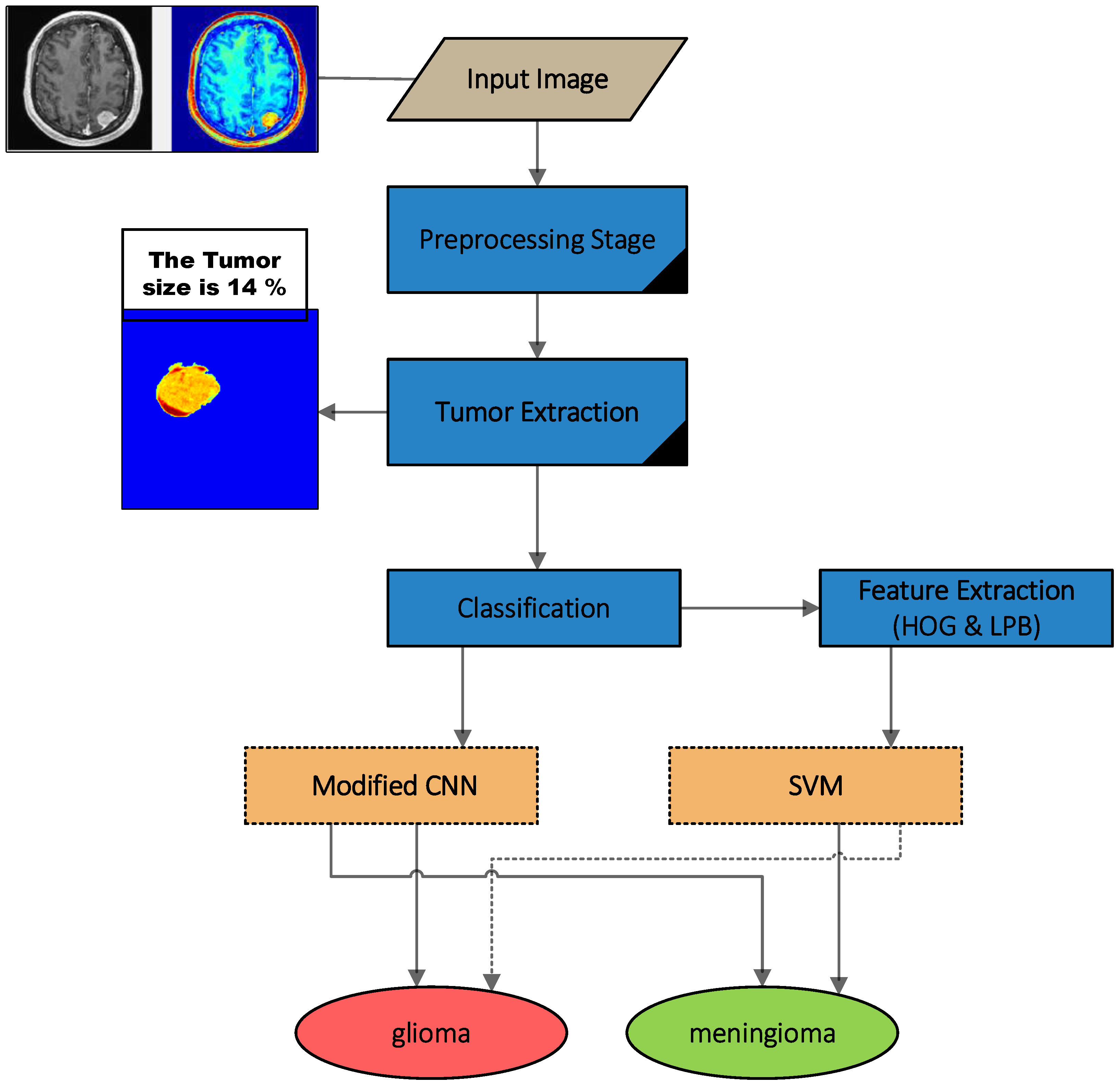
The image quality obtained through medical equipment dramatically influences the quality of processing results. As a direct result of the technological requirements of the devices, the resulting images (or sets of photographs) often display substantial noise. Methods for detecting and separating brain tumors are diverse. Our presented algorithmic approach focuses on segmenting objects with high precision and using features (in this case, brain tumors). In order to enhance the accuracy of diagnostic analysis on MRI images, we have proposed a technique for processing localized objects (tumors) on MRI images, as shown in
Figure 1. This is because the presence of noise in medical images can potentially distort the findings and conclusions of the analysis.
As shown in
Figure 1, the suggested model consists of the following steps:
Pre-processing: This step plays a crucial role in enhancing the quality of brain tumor MRI images, enabling more comprehensive and detailed analysis.
Tumor extraction: This stage includes the following two steps to extract the tumor:
Segmentation: Using the segmentation method, we can distinguish affected areas (tumors) from unaffected areas (brain). For the segmentation, we integrated the fuzzy clustering means and thresholding approaches (FCMT) to reach our enhanced method for segmentation.
Morphological Operation: This step includes deleting unwanted parts of the binary image and smoothing the boundary of segmented mass.
Feature Extraction: In this step, the HOG and LBP feature extraction methods are used to enhance the accuracy of segmented tumor classification.
Classification: This step includes the classification of the segmented tumor as cancerous or non-cancerous.
In order to assist their patients and determine what sort of tumor they have; doctors will typically provide them with a link to the image and a report outlining the image analysis. With the method we have shown, the system may be trained with less data while still providing reliable diagnoses for cancer patients. A report on the patient’s condition is prepared and utilized once the data have been verified.
In this case, the developed method and code draw on the backbone of an algorithm for recognizing tumors. While waiting, the relevant part of the document may be worked on. In the processing phase, analytical parameters are considered.
3.1. Dataset
In order to conduct an analysis, we examined over 150 scans of patients with brain tumors that were collected from the digital imaging communications in medicine (DICOM) [
20]. The researchers examined 150 images of brain tumors from the DICOM collection to get their conclusions. In addition, the Brain-web dataset is the second dataset that was used. This dataset was collected from the Euphrates Center for cancerous tumors in Iraq. It comprises comprehensive 3D brain MRI data. Within this collection, there were 48 images in total, and 15 of those images showed brain tumors.
The images in DICOM were grayscale and were resized to 256 × 256 px for processing. MRI scans of the brain are taken as input for all training and testing purposes. It is assumed that all the images input to the system are either benign (non-cancerous) or malignant (cancerous). The images are separated into two labeled folders for training and testing purposes. In the used database, 80% was used for training and 20% for testing, and we used the trainable model to test a new and private image to test set performance, and the trainable database did not include the same data for testing.
3.2. Feature Extraction
The pre-processed computed tomography data in this investigation yield both local and global properties. HOG and LBP feature extraction methods are described in detail in the following subsections.
3.2.1. HOG Features
Object recognition systems use the histogram of oriented gradients to classify images (HOG). Different gradient orientations are counted in a given area to find out how often they appear in medical imaging. With the help of the HOG feature extraction plugin, gathering such features is easy. Due to the inherent simplicity of the calculations, it is a significantly faster and more efficient feature descriptor than SIFT and LBP. In addition, HOG features have been demonstrated to be promising as actionable detection descriptors. Several applications may be discovered for this method in the realm of computer vision, namely in the study of image processing. It is possible that HOG will be utilized to define the picture’s form and style. Specifically, 4 × 4 pixel cells were used to analyze the picture and their orientation was used to determine where the edges were. Histograms may be re-scaled to increase precision [
13,
21].
When defining the distribution of intensity changes or data, the histogram of directional gradients may be used to define the look and shape of a nearby item. Each cell in the image may then have its own individual gradient direction histogram generated for it. Next, we apply support vector machine classification to assign labels to the recovered pictures and classify the fashion items in the F-MNIST dataset. Before training a classifier and performing an evaluation, the generated picture samples need to undergo some pre-processing in order to eliminate noise artifacts. Improved feature vectors for use in classifier training may be possible with proper pre-processing. Thorough pre-processing may increase the proportion of accurate classifications and identifications. The suggested research makes use of feature extraction based on HOGs to help in the identification of fashion items. The optimal width for HOG feature extraction is 2828 pixels [
22,
23].
There are four main methods for doing block equalization. A small constant (e) is placed in front of V, which represents all the histograms in a given block, and the non-normalized vector V is used to represent all the histograms in this block (the exact value, hopefully, is unimportant). After that, you may choose an adjustment factor from the following list:
L2-hys:
L2-normal followed by clipping (limiting the maximum values of
v to 0.2) and renormalizing, as in
Taking the L2-normal, compressing the result, and then renormalizing may be used to compute the L2-his method. On the other hand, the wide variances in the depth of field lead to a wide range of gradient magnitudes. To solve this problem, the histograms of each cell are normalized by combining neighboring cells into a bigger block. Finally, the HOG-based bounding boxes are generated by joining all of the selected CT slices.
3.2.2. LBP Features
The look of an image surrounding each individual pixel is characterized by what is termed a “Local Binary Pattern” (LBP). The premise behind simple normalization is that textures transmit micro-scale properties such as a pattern and the intensity of that pattern. The operator utilizes a 3-pixel-by-3-pixel image block for nearby binary patterns. The center pixel is labeled by thresholding its value, multiplying it by the power of two, and then stringing the results together. Since the area around the center consists of 8 pixels, there are 2
8 = 256 different labels that may be constructed by looking at the gray levels of both the center and the surrounding region. The central tendency and dispersion of the LBP features of an image are also considered during classification. A grayscale picture may be transformed into a numeric matrix using an LBP, which acts at the pixel level [
22]. This label matrix explains the different elements. To do this, we tell the system to find a mapping representation of the texture that works for what we are looking for. These types of visual descriptors are generally utilized in resumes because they help convey the message swiftly. Using HOG feature descriptors results in a significant performance gain.
LBP is a feature descriptor that is very useful for classifying textures. It is essential to think about texture while reading CT scans. It has been discovered that LBP is a potent extension for classification issues because of its invariance to grayscale and rotation [
24]. The radius
N surrounding the central pixel is what determines the textural properties based on LBP sampling stations (neighborhood pixels)
where
R is the radius of the circle and
N is the number of data points measured there. Quantization of angular space, governed by
R, determines the density of
LBP pixels. Therefore, these two aspects have a considerable impact on categorization precision. Pixel
k values are denoted by
x(
k), whereas pixel
C values are denoted by
x(
C). Invariance against grayscale and rotation for
LBP is ensured by the function
s(
x). If the value of
s(
x) is greater than or equal to the value of pixel
x(
k), then the value of
s(
x) is 1. In all other cases,
s(
x) equals 0.
3.3. Tumor Classification Using SVM Model
The prediction of tumors on medical images using extracted characteristics has been achieved using the SVM classifier (LPB and HOG). Non-probabilistically assigning new instances to one of two groups, the SVM is a binary linear classifier trained using a collection of examples pre-divided into categories. Support vector machines may be used to construct hyperplanes and hyperplane sets for classification tasks in high or infinite dimensional space. SVMs are an effective supervised learning approach used in machine learning to discover patterns in data. If sufficient separation and the maximum distance to neighboring training data of any category are attained, the hyperbolic plane may be reached. Generalization mistakes may be mitigated by increasing the margin of error. The support vector machine may be helpful in many different types of recognition tasks, such as facial recognition, textual task completion, and others. When put to action in realistic situations, it succeeds admirably [
25]. In this part of the study, we train and test using the SVM. The method was applied to the fashion pictures in the F-MNIST database, classifying them in HOG feature space using a multiclass support vector machine classifier. Rows of 1296 by 1296 HOG features are used to fill the whole feature space.
Rather than creating multiple binary classifiers, a more logical approach is to employ a single optimization technique for effectively categorizing multiple classes [
26,
27]. By utilizing these techniques, all k-binary SVMs can be simultaneously learned, ensuring a distinct objective variable and maximizing the separation between each category and the remaining items in a k-class problem. Assuming a labeled training set,
of cardinality l, where
and W is the weight, the formulation proposed in [
22] is given as follows:
The result of the decision is:
3.4. Tumor Classification Using CNN Model
Through our research, we discovered that it is challenging to recognize photographs with tiny features (as the tumor is a glioma or meningioma). The categorization model should not be very deep like Res-Nets or Res-Next [
12] models, but rather have a framework that can catch and learn subtle changes.
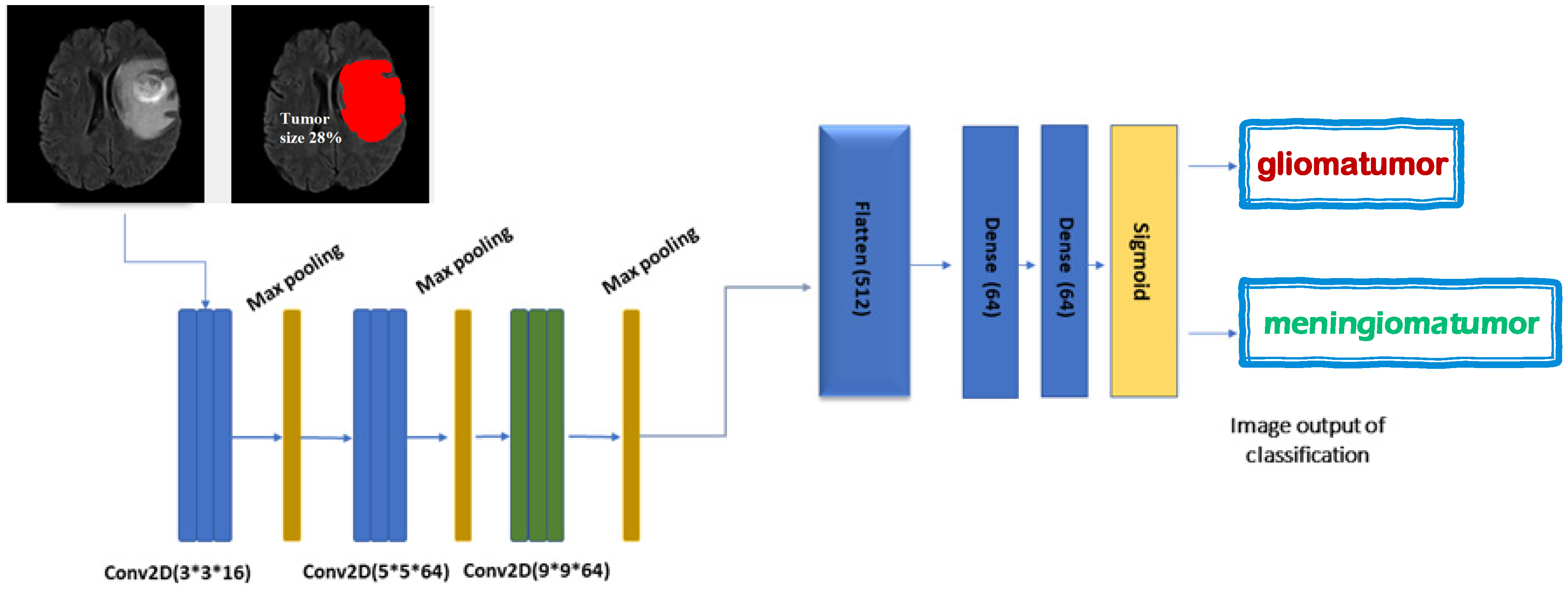
Figure 2 is a diagrammatic representation of the research’s recommended model. In particular, four convolutional layers are used in the proposed model. The batch normalization approach is used to normalize the inputs, which has additional advantages such as reducing the training time and improving the model’s stability. Leaky-Re-LU is a variant of the original Re-LU technique that provides protection to neurons as they leave the cell. The Max-pool procedure is used in all of our pooling procedures. Max-pool picks the greatest value within the zone given by its filter to minimize an input [
28]. The suggested model is able to classify two groups simultaneously, whether they are glioma tumors or meningiomas, or ordinary tumors. The classification job for brain tumors, whether glioma or meningioma, is performed using the same model. Finally,
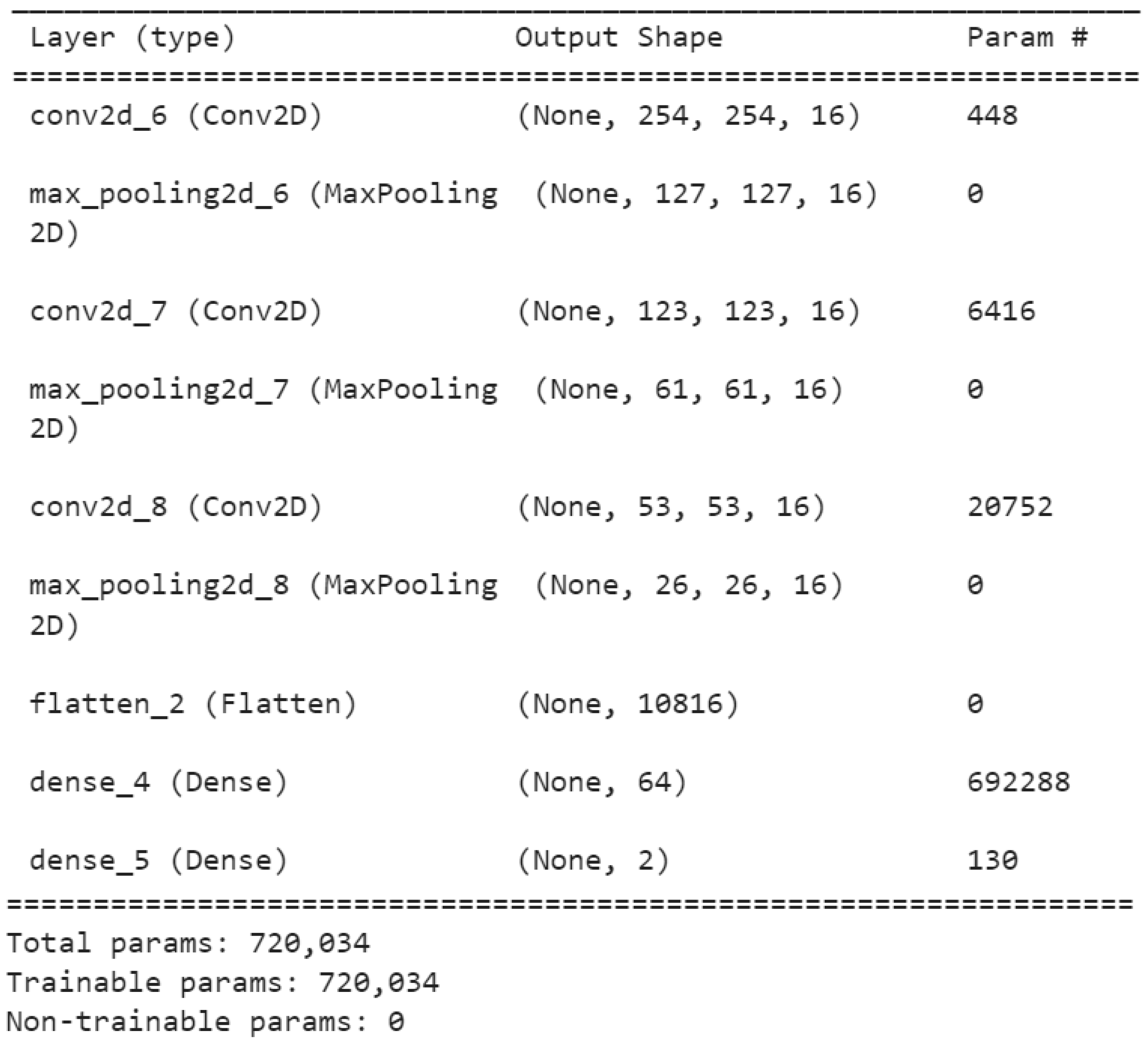
Figure 3 describes the layers and parameters used in the model. The developed deep learning model has 1,050,226 parameters. The Adam optimizer has been used to create weight updates, a cross-entropy loss function, and selective learning.
The purpose of using this model is to assist radiologists in prioritizing glioma-tumor or meningioma-tumor patients for testing and treating infections based on their unique etiology. With these needs in mind, we created the CNN-MRI architecture, comprising three parallel layers with 16, 64, and 64 filters in each layer, all with different sizes (3 by 3, 5 by 5, and 9 by 9). The coevolved pictures are then subjected to batch normalization and the rectified linear unit, followed by two types of pooling operations: average pooling and maximum pooling. The rationale for employing different filter sizes is to identify local features with 3-by-3 filters and somewhat global features with 9-by-9 filters, while the 5-by-5 filter size detects what the other two filters missed.
4. Results and Discussion
In this study, we employed two datasets for analyzing objects, specifically brain tumor extraction and prediction, differentiating between glioma and meningioma tumors. The first dataset utilized was the digital imaging dataset (DICOM) [
29,
30]. A total of 150 brain tumor images from the DICOM dataset were reviewed and analyzed by the researchers.
Additionally, we used the brain tumor dataset [
31] for this study as an extra dataset for model training. Researchers from Nanfang Hospital, General Hospital, and Tianjin Medical University in China created this dataset. They used a database of pictures consisting of a collection of slices, each of which had an individual magnetic resonance imaging (MRI) scan obtained between 2005 and 2010. The first online version was released in 2015, and the most current was finished in 2017 [
32,
33]. Pituitary malignancies, meningiomas, and gliomas all accounted for 1426 slices, whereas 708 depicted meningiomas (930 images). Scans were acquired in three planes from 233 patients: sagittal (1025 images), axial (994 images), and coronal (1045 images).
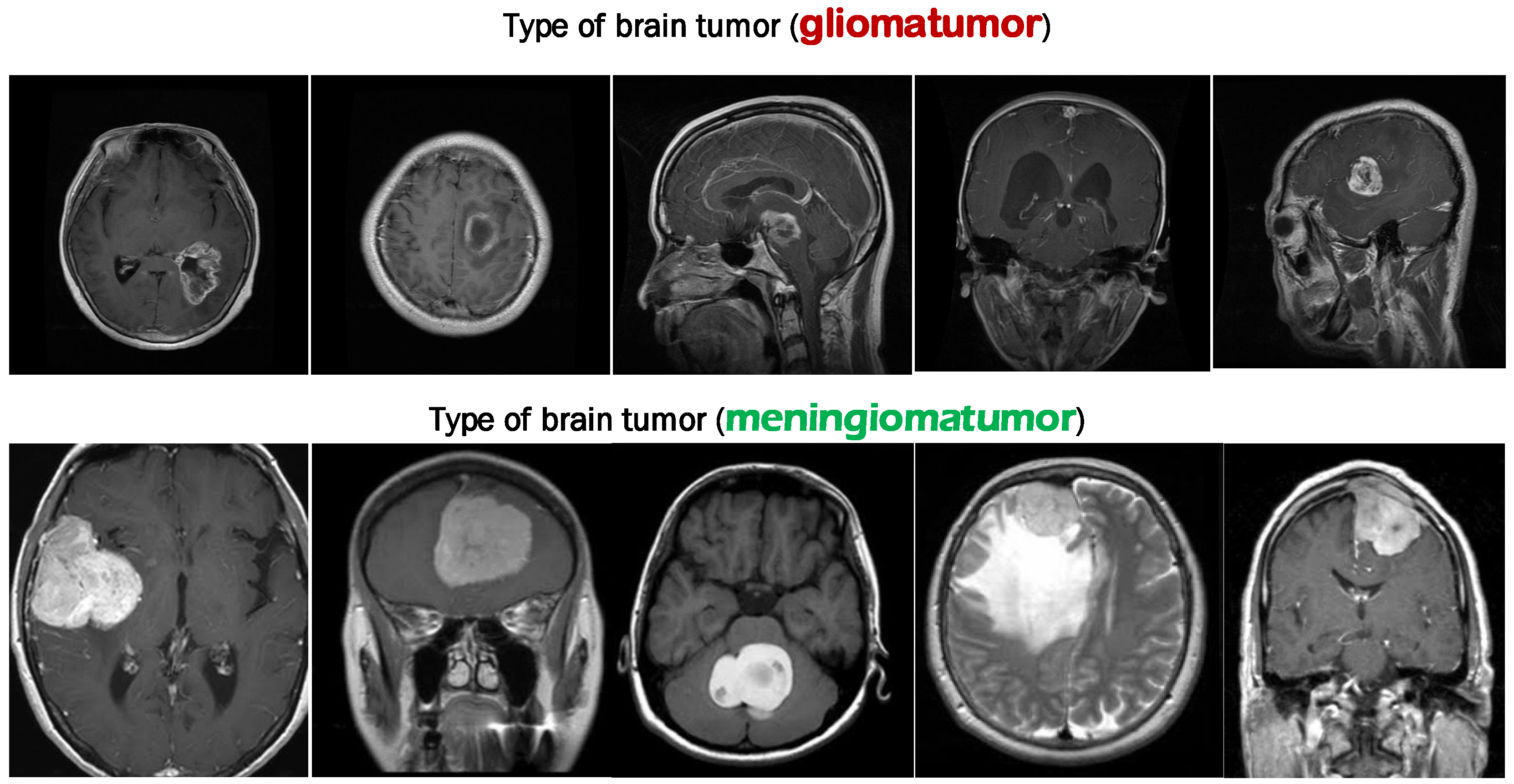
Figure 4 shows several different types of cancer on different axes. The edges of each tumor are a vivid shade of crimson. Each person is imaged an undetermined number of times.
We aimed to demonstrate that the modest architecture’s performance was on par with that of larger, more involved designs. Reduced time and energy spent on image processing are two benefits of using an FCMT to differentiate between infected and healthy brain tissue and tumors. This is an important issue to fix since it hinders the system’s use in clinical diagnostics and on software platforms where resources are scarce. The system must be adaptable if it is to be utilized in routine clinical diagnosis. The presented method outperforms previous recently published models, although our algorithm still has certain drawbacks when dealing with tumor volumes larger than one-third of the whole brain. This is because as the tumor becomes larger, the predicted area decreases, resulting in worse extracting features. The training was conducted on a joint set of MRI images (from the digital imaging in medicine (DICOM) dataset) to evaluate the accuracy of the SVM classifiers on which the MRI scan with tumor or not. The results and descriptions are shown in
Table 1 for the classification of brain tumors.
The average classification accuracy of the experimental studies is 97% with combined feature extraction. As can be noted from
Table 1, the meningioma tumor prediction accuracy was higher than the glioma tumor, with an accuracy of 93% on images with glioma tumors and 100% on images of meningioma tumor. The errors in the prediction of glioma tumors in MRI images are about 6% with combined feature extraction.
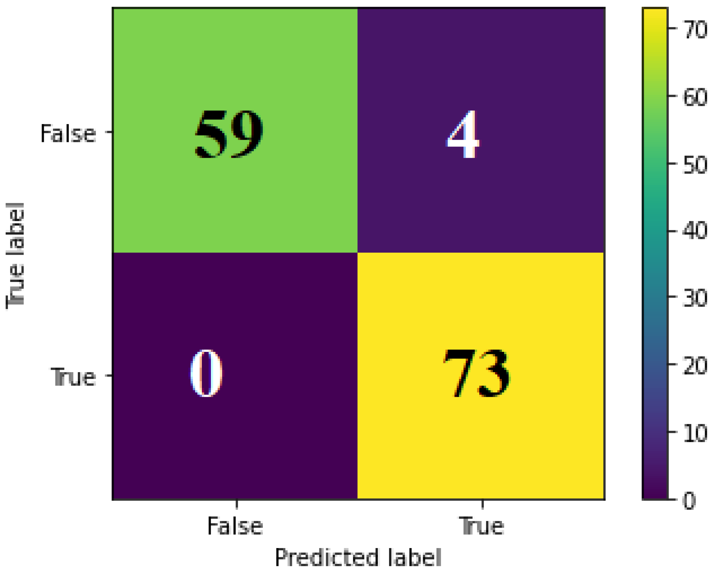
Figure 5 shows the confusion matrix of tumor prediction with HOG features and combined features (HOG + LPB).
From
Figure 5, we can see that the modified methodology for tumor prediction (combination of features HOG and LPB) is more accurate than using HOG features. The error rate by using a combination of LPB and HOG is 3%, while the usual method is 11%.
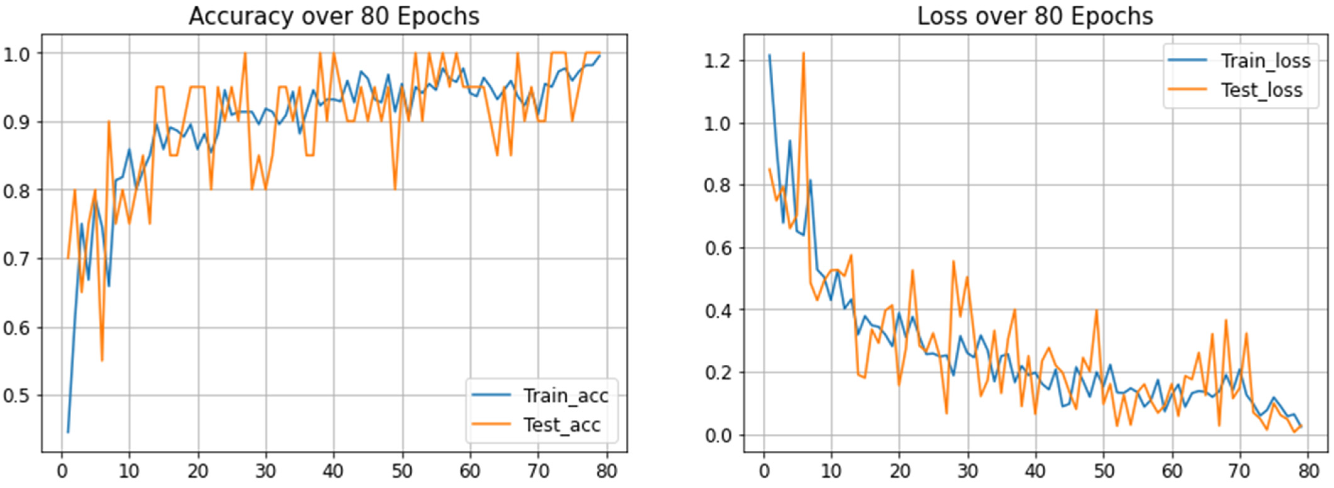
Figure 6 shows the training and testing accuracy over 80 epochs, with four layers on a modified convolution neural network (MCNN).
The performance accuracy of modified CNN for tumor classification on the BRATS 2018 dataset [
34,
35,
36] (glioma tumor or meningioma tumor) using a matrix of precision, recall, and f1-score for the evaluation model is shown in
Table 2.
The average modified CNN classification accuracy of the experimental studies is 98%, as can be noted from
Table 2; the tumor prediction accuracy was high, especially for meningioma tumors. The percentage of errors in the prediction of glioma tumors in MRI images is about 4%, and the prediction of meningioma tumors is 1%.
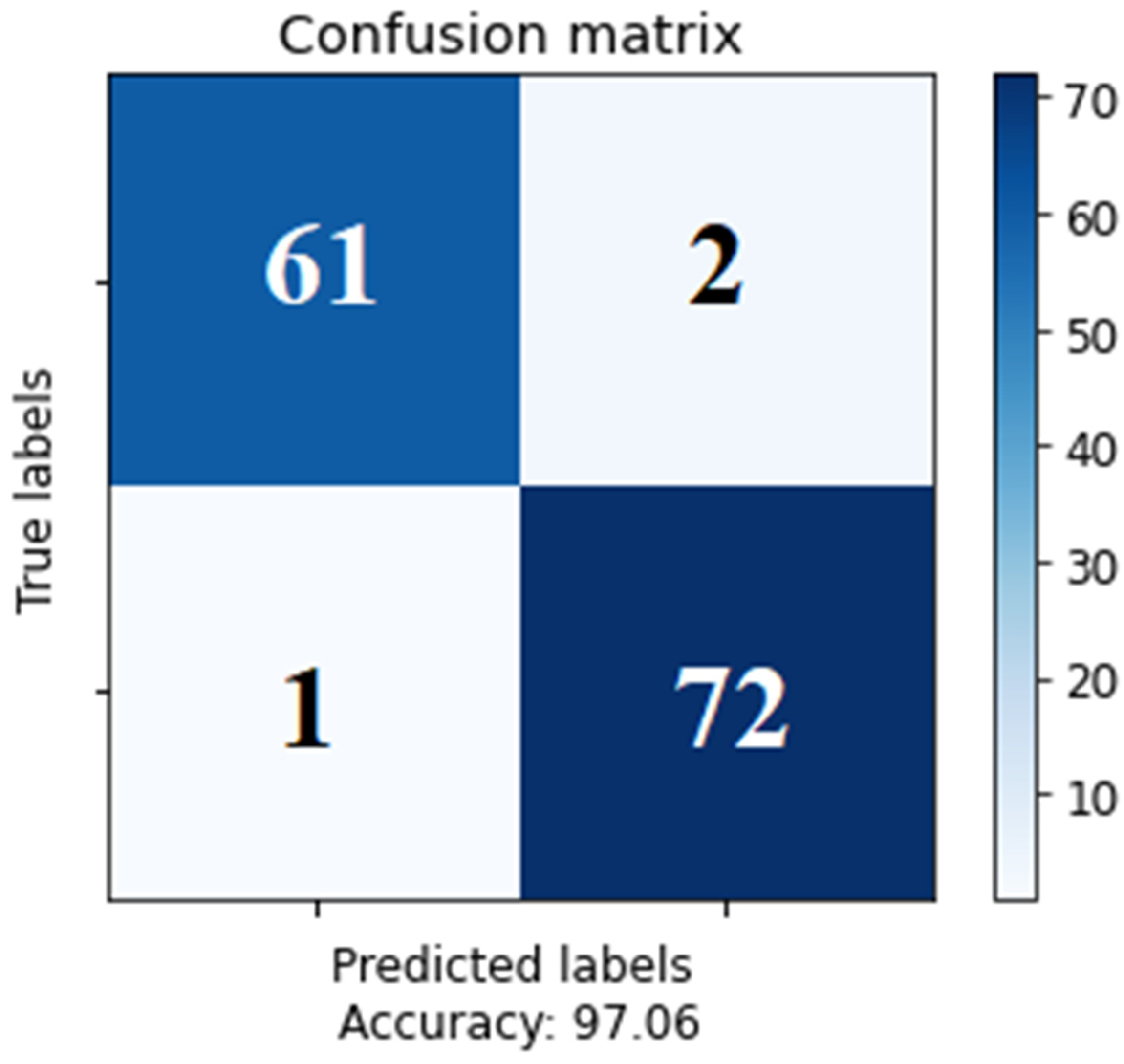
Figure 7 shows the confusion matrix of the tumor using a modified CNN classifier (glioma tumor or meningioma tumor) on the BRATS 2018 dataset. As can be seen from the results, the proposed methods of deep learning for the brain tumor diagnosis analysis using the SVM with combined features of LBP and HOG resulted in 100% accuracy for meningioma tumor detection. While the modified CNN model resulted in 98% accuracy, combining HOG and LBP features is more effective in detecting meningioma tumors. Moreover, the accuracy of SVM with single feature extraction (HOG or LBP) is less than 90%. As a result, we can see from
Table 3 that the accuracy reached by our study is better than the related research in the field.
5. Conclusions and Future Work
The analysis of brain tumor scans is often performed manually by doctors. Manually analyzing brain scans is laborious and is becoming more irrelevant as our understanding of the brain expands. Alternatively, automated segmentation and categorization make neurologists’ jobs easier by speeding up the decision-making process. Recent advances in the segmentation and prediction of brain tumor MRI images have been made possible via the use of deep learning algorithms. Despite this, MRI is still a complex topic where additional study is needed. Medical practitioners benefit substantially from segmentation and classification procedures since it expedites data analysis and provides a second opinion based on automated findings.
This article focuses on the use of machine learning to detect, characterize, and categorize malignant tumors (including gliomas and meningiomas). Image processing methods pioneered by FCMT, such as contrast enhancement, are used in tumor segmentation. Features are extracted using LBP and HOG. All of these characteristics come together to form an ensemble. In order to train the neural network, this Ensemble Features set is subjected to convolutional training. The accuracy of an SVM merged with HOG and LPB features is shown to be 99.9%, whereas that of a retrained CNN model is 98%. Less than 2% of errors are discovered. To enhance the study’s outcomes, incorporating ensemble classification approaches, such as employing a convolutional neural network (CNN) with diverse layer configurations or a deep convolutional neural network (DCNN), may yield superior results.
Our model was trained and tested using two datasets: DICOM and the Brain-web dataset; this could limit the generalizability of the trained models to different datasets. Therefore, we plan to train and test our model using more datasets.
Author Contributions
Conceptualization, N.T.A.R. and M.S.; methodology, N.T.A.R., R.M.M. and M.S.; software, R.M.M. and A.A.H.; validation, A.A.H., N.L.F. and G.A.; formal analysis, N.L.F. and G.A.; investigation, A.A.H. and M.S.; data curation, N.T.A.R. and R.M.M.; writing—original draft preparation, N.T.A.R., R.M.M. and A.A.H.; writing—review and editing, N.L.F., G.A. and M.S.; visualization, N.L.F. and G.A. All authors have read and agreed to the published version of the manuscript.
Funding
This research received no external funding.
Data Availability Statement
Not applicable.
Conflicts of Interest
The authors declare no conflict of interest.
References
- Biratu, E.S.; Schwenker, F.; Ayano, Y.M.; Debelee, T.G. A survey of brain tumor segmentation and classification algorithms. J. Imaging 2021, 7, 179. [Google Scholar] [CrossRef] [PubMed]
- El-Dahshan, E.-S.A.; Hosny, T.; Salem, A.-B.M. Hybrid intelligent techniques for MRI brain images classification. Digit. Signal Process. 2010, 20, 433–441. [Google Scholar] [CrossRef]
- Das, S.; Chowdhury, M.; Kundu, M.K. Brain MR image classification using multiscale geometric analysis of ripplet. Prog. Electromagn. Res. 2013, 137, 1–17. [Google Scholar] [CrossRef]
- Hamad, Y.A.; Seno, M.E.; Al-Kubaisi, M.; Safonova, A.N. Segmentation and measurement of lung pathological changes for COVID-19 diagnosis based on computed tomography. Period. Eng. Nat. Sci. (PEN) 2021, 9, 29–41. [Google Scholar] [CrossRef]
- Al-Okaili, R.N.; Krejza, J.; Woo, J.H.; Wolf, R.L.; O’Rourke, D.M.; Judy, K.D.; Poptani, H.; Melhem, E.R. Intraaxial brain masses: MR imaging-based diagnostic strategy—Initial experience. Radiology 2007, 243, 539–550. [Google Scholar] [CrossRef] [PubMed]
- Jiang, J.; Wu, Y.; Huang, M.; Yang, W.; Chen, W.; Feng, Q. 3D brain tumor segmentation in multimodal MR images based on learning population- and patient-specific feature sets. Comput. Med. Imaging Graph. 2013, 37, 512–521. [Google Scholar] [CrossRef]
- Ortiz, A.; Górriz, J.M.; Ramírez, J.; Salas-Gonzalez, D. Improving MRI segmentation with probabilistic GHSOM and multiobjective optimization. Neurocomputing 2013, 114, 118–131. [Google Scholar] [CrossRef]
- Zotin, A.; Hamad, Y.; Simonov, K.; Kurako, M.; Kents, A. Processing of CT Lung Images as a Part of Radiomics. In International Conference on Intelligent Decision Technologies; Springer: Singapore, 2020; pp. 243–252. [Google Scholar]
- Chen, M.; Yan, Q.; Qin, M. A segmentation of brain MRI images utilizing intensity and contextual information by Markov random field. Comput. Assist. Surg. 2017, 22, 200–211. [Google Scholar] [CrossRef]
- Raja, P.S.; Rani, A.V. Brain tumor classification using a hybrid deep autoencoder with Bayesian fuzzy clustering-based segmentation approach. Biocybern. Biomed. Eng. 2020, 40, 440–453. [Google Scholar] [CrossRef]
- Hamad, Y.A.; Simonov, K.V.; Naeem, M.B. Detection of brain tumor in MRI images, using a combination of fuzzy C-means and thresholding. Int. J. Adv. Pervasive Ubiquitous Comput. (IJAPUC) 2019, 11, 45–60. [Google Scholar] [CrossRef]
- Deepak, S.; Ameer, P. Brain tumor classification using deep CNN features via transfer learning. Comput. Biol. Med. 2019, 111, 103345. [Google Scholar] [CrossRef]
- Hamad, Y.A.; Simonov, K.; Naeem, M.B. Brain’s tumor edge detection on low contrast medical images. In Proceedings of the 2018 1st Annual International Conference on Information and Sciences (AiCIS), Fallujah, Iraq, 20–21 November 2018; pp. 45–50. [Google Scholar]
- Hamad, Y.A.; Qasim, M.N.; Rashid, A.A.; Seno, M.E. Algorithms of Experimental Medical Data Analysis. In Proceedings of the 2020 International Conference on Computer Science and Software Engineering (CSASE), Duhok, Iraq, 16–18 April 2020; pp. 112–116. [Google Scholar]
- Garg, G.; Garg, R. Brain tumor detection and classification based on hybrid ensemble classifier. arXiv 2021, arXiv:2101.00216. [Google Scholar]
- Kesav, N.; Jibukumar, M. Efficient and low complex architecture for detection and classification of brain tumor using RCNN with two channel CNN. J. King Saud Univ.-Comput. Inf. Sci. 2021, 34, 6229–6242. [Google Scholar] [CrossRef]
- Khan, M.F.; Khatri, P.; Lenka, S.; Anuhya, D.; Sanyal, A. Detection of Brain Tumor from the MRI Images using Deep Hybrid Boosted based on Ensemble Techniques. In Proceedings of the 2022 3rd International Conference on Smart Electronics and Communication (ICOSEC), Ttichy, India, 20–22 October 2022; pp. 1464–1467. [Google Scholar]
- Alanazi, M.F.; Ali, M.U.; Hussain, S.J.; Zafar, A.; Mohatram, M.; Irfan, M.; AlRuwaili, R.; Alruwaili, M.; Ali, N.H.; Albarrak, A.M. Brain tumor/mass classification framework using magnetic-resonance-imaging-based isolated and developed transfer deep-learning model. Sensors 2022, 22, 372. [Google Scholar] [CrossRef]
- Gómez-Guzmán, M.A.; Jiménez-Beristaín, L.; García-Guerrero, E.E.; López-Bonilla, O.R.; Tamayo-Perez, U.J.; Esqueda-Elizondo, J.J.; Palomino-Vizcaino, K.; Inzunza-González, E. Classifying Brain Tumors on Magnetic Resonance Imaging by Using Convolutional Neural Networks. Electronics 2023, 12, 955. [Google Scholar] [CrossRef]
- Rutherford, M.; Mun, S.K.; Levine, B.; Bennett, W.; Smith, K.; Farmer, P.; Jarosz, Q.; Wagner, U.; Freyman, J.; Blake, G.; et al. A DICOM dataset for evaluation of medical image de-identification. Sci. Data 2021, 8, 183. [Google Scholar] [CrossRef]
- Gawande, S.S.; Mendre, V. Brain tumor diagnosis using deep neural network (dnn). Int. J. Adv. Res. Electr. Electron. Instrum. Eng. 2017, 5, 10196–10203. [Google Scholar]
- Arunkumar, N.; Mohammed, M.A.; Mostafa, S.A.; Ibrahim, D.A.; Rodrigues, J.J.; Albuquerque, V.H.C. Fully automatic model-based segmentation and classification approach for MRI brain tumor using artificial neural networks. Concurr. Comput. Pract. Exp. 2018, 32, e4962. [Google Scholar] [CrossRef]
- Kaplan, K.; Kaya, Y.; Kuncan, M.; Ertunç, H.M. Brain tumor classification using modified local binary patterns (LBP) feature extraction methods. Med. Hypotheses 2020, 139, 109696. [Google Scholar] [CrossRef]
- Amin, J.; Sharif, M.; Raza, M.; Saba, T.; Rehman, A. Brain tumor classification: Feature fusion. In Proceedings of the 2019 International Conference on Computer and Information Sciences (ICCIS), Sakaka, Saudi Arabia, 3–4 April 2019; pp. 1–6. [Google Scholar]
- Yang, J.; Chen, Z.; Zhang, J.; Zhang, C.; Zhou, Q.; Yang, J. HOG and SVM algorithm based on vehicle model recognition. In MIPPR 2019: Pattern Recognition and Computer Vision; SPIE: Bellingham, WA, USA, 2020; Volume 11430, pp. 162–168. [Google Scholar]
- Sachdeva, J.; Kumar, V.; Gupta, I.; Khandelwal, N.; Ahuja, C.K. Multiclass brain tumor classification using GA-SVM. In Proceedings of the 2011 Developments in E-Systems Engineering, Dubai, United Arab Emirates, 6–8 December 2011; pp. 182–187. [Google Scholar]
- Hamad, Y.A.; Kadum, J.; Rashid, A.A.; Mohsen, A.H.; Safonova, A. A deep learning model for segmentation of COVID-19 infections using CT scans. AIP Conf. Proc. 2022, 2398, 050005. [Google Scholar]
- Hamad, Y.A.; Simonov, K.; Naeem, M.B. Breast cancer detection and classification using artificial neural networks. In Proceedings of the 2018 1st Annual International Conference on Information and Sciences (AiCIS), Fallujah, Iraq, 20–21 November 2018; pp. 51–57. [Google Scholar]
- Alfonse, M.; Salem, A.B.M. An automatic classification of brain tumors through MRI using support vector machine. Egypt. Comput. Sci. J. 2016, 40, 11–21. [Google Scholar]
- Abdel-Maksoud, E.; Elmogy, M.; Al-Awadi, R. Brain tumor segmentation based on a hybrid clustering technique. Egypt. Informatics J. 2015, 16, 71–81. [Google Scholar] [CrossRef]
- Cheng, J.; Brain Tumor Dataset. Science Data Bank. 8 November 2022. Available online: https://www.scidb.cn/en/detail?dataSetId=faa44e0a12da4c11aeee91cc3c8ac11e (accessed on 1 January 2023).
- Bahadure, N.B.; Ray, A.K.; Thethi, H.P. Image analysis for MRI based brain tumor detection and feature extraction using biologically inspired BWT and SVM. Int. J. Biomed. Imaging 2017, 2017, 9749108. [Google Scholar] [CrossRef] [PubMed]
- Mohan, G.; Subashini, M.M. MRI based medical image analysis: Survey on brain tumor grade classification. Biomed. Signal Process. Control 2018, 39, 139–161. [Google Scholar] [CrossRef]
- Menze, B.H.; Jakab, A.; Bauer, S.; Kalpathy-Cramer, J.; Farahani, K.; Kirby, J.; Burren, Y.; Porz, N.; Slotboom, J.; Wiest, R.; et al. The multimodal brain tumor image segmentation benchmark (BRATS). IEEE Trans. Med. Imaging 2014, 34, 1993–2024. [Google Scholar] [CrossRef] [PubMed]
- Bakas, S.; Akbari, H.; Sotiras, A.; Bilello, M.; Rozycki, M.; Kirby, J.S.; Freymann, J.B.; Farahani, K.; Davatzikos, C. Advancing The Cancer Genome Atlas glioma MRI collections with expert segmentation labels and radiomic features. Sci. Data 2017, 4, 170117. [Google Scholar] [CrossRef]
- Bakas, S.; Reyes, M.; Jakab, A.; Bauer, S.; Rempfler, M.; Crimi, A.; Jambawalikar, S.R. Identifying the best machine learning algorithms for brain tumor segmentation, progression assessment, and overall survival prediction in the BRATS challenge. arXiv 2018, arXiv:1811.02629. [Google Scholar]
| Disclaimer/Publisher’s Note: The statements, opinions and data contained in all publications are solely those of the individual author(s) and contributor(s) and not of MDPI and/or the editor(s). MDPI and/or the editor(s) disclaim responsibility for any injury to people or property resulting from any ideas, methods, instructions or products referred to in the content. |
© 2023 by the authors. Licensee MDPI, Basel, Switzerland. This article is an open access article distributed under the terms and conditions of the Creative Commons Attribution (CC BY) license (https://creativecommons.org/licenses/by/4.0/).


 ,
, 


