1. Introduction
Machine learning is a field of artificial intelligence, which deals with systems and algorithms able to automatically detect patterns in data. These systems and algorithms try to replicate the functioning of the human brain, which is able to learn general laws about a given system starting from a limited number of related examples. Our contribution consists of the proposal of a rule-based machine learning method designed to optimize a water distribution network (WDN). More specifically, the proposed method allows us to optimize the control of the pumps in real time. Even though we will focus on this application, we would like to mention that, in principle, the proposed algorithm could be applied in any other scenario involving a real-time optimization problem. The development of a support decision tool for this application is motivated by the fact that it is very difficult for an operator to predict the effect of status changes on a set of pumps across the whole system over time. In fact, both the overall energy consumption and the system quality of service must be taken into account at the same time for the optimization. We may define quality of service according to measurements related to water quality (such as chlorine concentration on water age) but, in the following, we will focus on a definition of quality of service based on the compliance of pressure levels in the network with target pressure ranges: the relevance of this element in water main operations is discussed, for example, in [
1]. Operations are usually based on simple correlations known a priori. For example, if the aim is to improve the quality of service (QoS ) in a specific point of the network, the operator may switch on a pump in a nearby pumping station that is known to be related to the pressure in that point.
It is, however, not always so easy to take other correlations into account empirically; for example, correlations related to interactions among pumping stations, or to effects associated with more distant pumping stations.
For this reason, a machine learning approach could help in making better predictions by also considering more complex correlations among variables. Most machine learning approaches provide models in the form of complex mathematical functions, which leads to a number of significant limitations: (a) it is difficult to understand the cause–effect relationships and therefore (b) it is difficult to understand which drivers should be changed to improve network behavior. For this reason, a rule-based approach is proposed, leading to a better understanding of the network behavior and its key drivers. In this paper, rule-based control (RBC) is proposed to optimize a WDN. The two steps constituting the proposed method are the following:
The extraction of a rule-based model that allows us to predict the future status of the network (e.g., pressure constraints will not be fulfilled/energy consumption will be excessive/a good status of the network);
The use of the extracted model to generate controls to change the status of the pumps in order to match rules that predicted the desired status of the network.
The proposed pipeline is currently used by one of the biggest water main systems in Italy (Milan water main). Its performance in the long term, in terms of energy saving, is under evaluation and is being compared with other state-of-the-art techniques.
The structure of the paper is the following:
Section 2 focuses on related work in this field,
Section 3.1 is dedicated to the description of the proposed modeling technique and
Section 3.2 shows how the use of this modeling technique allows us to develop and apply the innovative rule-based control algorithm.
Section 4 includes experimental results; conclusions follow.
2. Materials and Methods
In a water supply system, the source of water is generally a lake, a river or an underground aquifer. Water then flows through water treatment facilities so that it can be purified and is finally delivered to all the demand points. This defines, especially if the area to be covered by the water main is large, a complex network, constituted by many interconnected elements and sub-systems with different functions.
The quality of service may be determined by different criteria and parameters; for example, the quality of the water can be assessed. Another relevant objective of the water main system, which will be the target of our proposed technique in experiments, is to ensure that the water reaches every area of the network under a satisfactory pressure. In order to assess this and to optimize it, pressure sensors are distributed in the network and an optimal pressure range is defined for each of the monitored points.
When optimizing this, it must be taken into account that hydraulic pumps, which allow for the reaching of the goal, require energy to work, and the cost to power them represents a significant percentage of the overall cost of the system. Due to that, the ideal goal, widely explored in this field of research, is to ensure that the optimal ranges for pressure are met with the least possible energy consumption.
As observed in [
2], there is no single optimal choice of architecture that could be recommended to fit any water distribution control due to the existence of site-specific challenges. As previously mentioned, sensors shall be distributed in the network to allow for the acquisition of field measurements, while actuators allow us to actively control the distribution process according to the measurements and the prediction of the model about the future status of the water main system. The control of the network can be either supervised or entirely automatic.
Supervised control implies the intervention of a human operator who needs to confirm or modify the controls suggested by the model. Conversely, in an entirely automatic scenario, control actions are applied without any human intermediation. Considering that ensuring the correct behavior of a water main system is a very critical task, the entirely automatic solution is hard to pursue, at least as first step. Another distinction worth mentioning concerns the level at which the optimization of a water distribution network can happen. For example, optimizing can be interpreted as choosing the best solution for planning a new distribution system or for expanding an existing one: an extensive review of the most popular approaches for addressing the problem in this way was proposed in [
3]. To cite a few examples, [
4] used a meta-heuristic algorithm named
Shuffled Frog Leaping to determine optimal discrete pipe sizes for new pipe networks or for network expansions. In [
5], a local search was used to find the least expensive pipe configuration that satisfies hydraulic laws and customer requirements in a quick and transparent way.
The goal of the WDN operation optimization is to pick the best solution for pump and/or valve control in an existing network. The WDN operation optimization generates a schedule of pump operations either for a target time interval (e.g., a day or a week), or continuously, checking and possibly updating controls for the current steps and possibly for the future steps. In case the scheduling is fixed and does not change, we can also refer to the problem as a Pump Scheduling Optimization problem.
Since the solution is static, i.e., it does not need to be updated on a regular basis, computationally expensive methods can also be used to solve this kind of problem. Therefore, once the problem has been formulated, it is possible to find an optimal or near-optimal solution, which can then be used for scheduling the WDN. Scheduling optimization does, however, require that some boundary conditions, such as water demand, are fixed and known at the beginning of the scheduling period (e.g., a day) while, in a real-word scenario, the demand presents fluctuations that are difficult to predict ahead of time. Differences between estimated demand and the actual one can lead to bad optimization and, potentially, to failing to satisfy constraints.
Conversely, if the optimal solution is verified and, if needed, updated at each step, taking the input gathered at the current step into account, the problem is defined as Real Time Pump Optimization. The solution, in this case, happens at each time step: considering that we are speaking of a real-time application, computational efficiency in the determination of a (near) optimal solution is crucial.
In both cases, the optimization process aims to minimize the quantity/cost of energy consumed by pumps while ensuring that the network can meet quality of service constraints defined by the customer. In some studies, other objectives, such as the water quality and greenhouse gas emissions (GHGs), are also considered.
A relevant example of a controlled variable is WDN pressure. In this context, controllers were proposed starting from simple physical considerations on network behavior; for example, in [
6]. As an alternative, forecast techniques estimating the future state of the system can also be the input for the control layer. This kind of approach, for instance, was proposed in [
7,
8].
In [
9], a survey of methods for operation-level control of WDN pressure was reported. The methods proposed in the literature include mixed-integer linear programming as suggested by [
10] as well as a combination of optimization methods with machine learning approaches as in [
11,
12,
13].
In real-world applications, the most used metaheuristic search methods are
genetic algorithms (
GAs), which are inspired by Darwin’s theory on the biological processes of reproduction and natural selection. Since a GA simulates a biological process, it includes some randomness and different runs could lead to non-identical results; consequently, there is no guarantee that the GA reaches the optimal solution and it may stop at a local minimum. Nevertheless, some experiments have shown that, if the algorithm parameters are chosen correctly, the use of GAs could lead to near-optimal solutions, as shown in [
14]. Basically, all the variants of GAs are based on both the iterative generation of possible solution vectors and their evaluation based on a specific fitness score.
The method proposed in this paper allows for the real-time optimization of a network without imposing a physical model of the network. According to the four criteria defined by [
15], this is how it relates with state-of-the-art techniques:
Application area: The application area of RBC is “pump operation”, like the largest portion of the paper analyzed by Mala-Jetmarova (40%).
Optimization model: The optimization model used in this work considers a single objective (pump energy consumption) like the vast majority of models according to Mala-Jetmatova (84%). The test case considered 3 constraints (demand satisfied, nodes pressure, tanks level) but RBC allows us to deal with any number of constraints by changing the quality indicator.
Solution methodology: The RBC solution methodology is hybrid: the rule extraction step is stochastic, whereas the control step is deterministic. (in the literature, deterministic methods are 45.5% of the total).
Test network: For what concerns the test network, we used a mid-size network with approximately 400 demand nodes, whereas 80% of papers used a network with fewer than 100 nodes.
2.1. Optimization Model
Optimization consists of selecting the best values for some variables (called decision variables) to minimize or maximize a (set of) functions (called objectives) according to specific constraints. If an optimization problem includes only one objective, it is called single-objective programming; otherwise, it is called multi-objective programming.
In multi-objective optimization, it is usually impossible to find a single solution that minimizes (maximizes) all the objectives, so the result is consequently a set of nondominated solutions where ulterior improvements in one objective are not possible without worsening the others. Decision makers must then select the best option from the set of solutions.
For this reason, most of the literature on WDN operation optimization focuses on single-objective programming. If more criteria need to be optimized by design, they are usually combined into a single-objective function. Usually, the decision variables are the statuses of the pumps, which could be either binary (on/off) or continuous variables, if the pump includes some mechanism to tune the pressure of outgoing water.
Almost all the models in literature include the pump operating cost in the objectives, while other frequently used costs are the maintenance, usually estimated from the number of pump switches (e.g., [
16]), the water age (e.g., [
17]) and the GHG emissions (e.g., [
18]).
The problem is called linear programming if both the objectives and the constraints can be written as linear combinations of the decision variables; otherwise, it is called a non-linear programming problem. The WDN optimization problem in the literature is formulated both as a linear problem and as a non-linear problem.
A large variety of WDN operational constraints is present in the literature, and the most common ones concern pressure at nodes and levels of tanks. For instance, a linear regression model can be used to interpolate the relationship between pump status, tank levels, demand, pressure and energy in order to obtain an optimization model characterized by a linear objective and linear constraints (e.g., [
19]). Of course, introducing a linear model could induce an excessive simplification of the behavior of the system and therefore a reduction in the performance of the control.
In the following subsections, a short description of the main optimization models and solution methodologies is proposed.
2.2. Optimization Methods
An optimization method is a technique used to find a solution for an optimization model. The most common approach in this field is referred to as metaheuristic optimization.
A metaheuristic algorithm is a general-purpose algorithm that can be used to find a (sub)optimal solution for both linear and non-linear problems. Even if metaheuristic approaches do not guarantee that the optimal solution is retrieved, they are usually faster than deterministic methods and, therefore, they can also be used when the optimal solution cannot be obtained in a reasonable amount of time.
Notice that metaheuristic algorithms also aim at exploring the solution space by including some random decisions; thus, different executions could lead to different solutions even if they start from the same problem and set of parameters.
Exploring the solution space through metaheuristic approaches is usually combined with a hydraulic simulator that, at each iteration of the algorithm, tests the quality of the explored solution. The most commonly used heuristic search methods are
genetic algorithms (
GAs), which are described in
Section 2.3.
For real-time optimization, the use of hydraulic simulators is computationally expensive as shown in [
12]; consequently, a machine learning method can be used to capture knowledge from the hydraulic simulator.
For example, in [
13], a GA was combined with a
multilayer perceptron (
MLP), introduced in [
20]. In this approach, the MLP retrieves the status of each pump, the level of the tank and the expected water demand at time
t as inputs and returns the energy consumption, the level of each tank and the pressure of each node at time
, where
is the time period to be optimized. The GA then uses this information in place of the hydraulic simulator to find the best configuration according to the consumed energy and quality of the service.
The MLP is trained by means of a training set obtained by collecting a large set of possible behaviors from the hydraulic simulations of different realistic network situations. The software used for simulations is EPANET 2.0, introduced by [
21], one of the most widely used hydraulic simulators, which will also be referred to in the experimental section of the present paper.
However, MLPs are black boxes, i.e., classifiers whose behavior is difficult to explain. Recent trends in AI tends to prefer white boxes, i.e., classifiers whose behavior can be understood by a human: this approach is usually called explainable AI (XAI).
2.3. Genetic Algorithms
A genetic algorithm (GA) is a metaheuristic research method inspired by Darwin’s theory on the biological processes of reproduction and natural selection.
The method allows us to find high-quality solutions for complex problems, where traditional methods are not applicable or require excessive computational effort. Since a GA simulates a biological process, it includes some randomness, and different runs could lead to non-identical results; consequently, there is no guarantee that GA reaches the optimal solution and it may stop at a local minimum. Nevertheless, some experiments have shown that, if the algorithm parameters are chosen correctly, the use of GAs could lead to near-optimal solutions, as shown in [
14].
Different variants of GAs are used in the literature. Basically all of them are based on the iterative generation of possible solutions by means of the combination of elementary operations performed on the values of potential solution vectors. Borrowing the terminology from biology, the value of a variable is a gene, which may undergo a mutation (i.e., a random change) or a recombination with another solution, giving origin to a new offspring. Moreover, at each iteration, only some solutions are selected to optimize a fitness score.
In most GA applications for solving WDN operation optimization problems, the objectives and the constraints are not computed by closed-form expressions depending on the status of pumps. Usually, objectives and constraints are either produced by a hydraulic simulator or by a model that emulates the behavior of a simulator.
3. Theory/Calculation
3.1. Modeling
As mentioned in
Section 2, optimization methods require the management of several closed-form differential equations dealing with the physical laws that describe the behavior of the network or, alternatively, the use of hydraulic simulators that implicitly (and approximately) handle these relations.
In this paper, a different approach is proposed that allows us to perform optimization without the need for a physical model or a simulator. In fact, the relationships among parameters were implicitly derived from historical data by evaluating the effectiveness of network configurations used in the past in ensuring the quality of the WDS. Once the drivers leading to a good quality of the network are identified from historical data, it is possible to act on them to improve the current configuration quickly and with little computational cost. Due to this, the proposed approach does not need the definition since a set of solutions labeled as “good” or “bad” is sufficient to highlight the drivers that influence the quality of the network.
Thanks to these features, RBC could be an efficient alternative to exact optimization when it is not possible (or too computationally intensive) to predict the evolution of the network through closed differential equations or an accurate hydraulic simulator.
RBC aims at identifying and acting on a solution leading to “good configuration” and “bad configuration”. The definition of a “good solution” depends, of course, on the requirements and on the boundary conditions of the network; it is, however, possible to define the current performance of the network based on historical statistics. Consider a set
of historical data:
where
is the observed cost (e.g., the energy consumption per quantity of pumped water) for the considered configuration. We will refer to a solution of the problem as a set of settings of the network constituting the parameter vector
. In particular, the solution
is “good” with respect to historical data
if
, where
is the
q-th percentile (where
) of observed cost
in historical data
(the
q-th percentile is the minimum observed value in data that is greater or equal to a fraction
q of all the observed values). Otherwise, the solution is “bad”. For example, by setting
, a solution is considered good if its indicator is less than or equal to the median of the cost of past solutions, and is bad otherwise.
The goal of RBC is to produce solutions with a performance indicator smaller than . These solutions will constitute new historical data for future runs, and future runs will aim to further decrease the performance indicator. The value of is then expected to decrease progressively; in other words, when iterated several times, RBC should therefore lead to better and better solutions over time until reaching a value , which cannot be further improved. Ideally, if does not depend on external parameters and supposing that it is always possible to act on controllable variables, the optimization effect of RBC will decay over time as the steps toward an optimal solution become smaller and smaller. In a real-life situation, it may not be feasible to bring the output under the percentile acting on controllable variables.
Supposing that no other constraints are set for the WDN, the measure y computed on historical data, properly discretized, can be used as the output of a classification problem to make a prediction about the performance and its correlation with the network configuration.
However, the problem usually includes some operational constraints that define the quality of the system (i.e., pressure at nodes); therefore, a definition based only on energy efficiency is not suitable.
More specifically, in a typical WDN optimization problem, these indicators can be considered:
The efficiency indicator that corresponds to the cost in the unconstrained case, i.e., it is related to the energy consumption.
The quality indicator that represents the observed value of a penalty function accounting for the fulfillment of constraints.
Since the quality indicator is the primary objective for reaching a good solution, the criterion for evaluating if a solution is efficient considers
as the primary objective and
as the secondary objective.
where
is the subset of the
satisfying condition (
1). In the first place, a solution must have a good quality indicator, and the best solutions will also be characterized by a good efficiency indicator.
A single discrete indicator can therefore be defined with three possible classes:
Bad quality of the service () is the worst class and indicates that the constraints are poorly respected ;
Bad energy efficiency () is an intermediate class corresponding to fulfilled constraints but a high cost function ;
Good energy efficiency () is the best class in which constraints are respected and the efficiency indicator is low .
The dataset produced by this output definition phase is made of N examples and can be used as a training set for the learning phase of a rule-based classification model. In this context, the use of the XAI method is crucial because it allows us to not only make predictions, but also to have a clear insight about the cause–effect relationships.
This learning phase consists of using historical data to generate the model that describes the relationship between inputs (parameters of the WDN) and the output (performance of the WDN).
For the rule extraction step, the use of the logic learning machine (LLM) method is suggested. Notice that it is possible to perform the rule generation phase periodically (e.g., every day) so that changes in the behavior of the system are included in the created models.
The LLM is a clear box method based on the
switching neural network (
SNN) model, introduced by [
22], which generates a set of intelligible rules through Boolean function synthesis. Briefly, the LLM transforms the data into a Boolean domain where some Boolean functions (namely one for each output value) are reconstructed starting from a portion of their truth table with the method described in [
23]. The Boolean functions are then converted back into intelligible rules involving the original variables:
where
is the conjunction of a set of conditions on the input variables (e.g., the pressure, the time of the day, etc.) and
contains the output value (i.e., the performance of the network) corresponding to
.
Competing techniques, such as decision trees, introduced by [
24], usually produce complex rulesets (i.e., with many splits) that are too dependent on the initial splits. Moreover, the effectiveness of rule-based optimization depends on the “completeness” of the set of rules. In other words, as the next sections will clarify, optimization is searching for conditions leading to good configurations; thus, it is important that (almost) all the possible correlations are retrieved by the classification algorithms in order to increase the chance of having at least one available and attainable good configuration. On the contrary, due to the divide-and-conquer approach of DT, even if they are more complex, the number of rules is usually reduced and each vector
satisfies only one rule; for this reason, in several situations, it is possible that no good configurations can be achieved from the current situation. A random forest (RF) model, proposed by [
25], would produce a larger ruleset containing redundant rules, where it is also more complex for the RF to apply changes in order to improve a solution. In addition, since it is not constrained to a tree structure, the LLM is able to integrate intelligible rules based on WDN expert knowledge, increasing the level of customization of the solution. However, if a DT or RF are used, the RBC approach can be applied after having converted the tree (or the ensemble of trees) into a set of rules.
Whatever the rule generation method used, the rules can be evaluated, introducing some quality measures related to their ability to describe the available data.
A generic rule
can be seen as a couple
, where
is a vector of conditions and
is the output in its consequence. Let
be the attribute associated with a condition
. An example
is said to be
covered by
r (denoted by
) if it satisfies all the conditions in
. Vice versa,
means that
is not covered by
. The
covering of
r is the fraction of cases
in the training set having
and input
covered by
r:
where
is the number of cases in the training set having output
and satisfying all the conditions in
and
is the number of cases having output
, while the
error of
r is the fraction of the example in the training set having output
covered by
r.
where
is the number of cases in the training set having an output different from
and covered by
r and
is the number of cases where the output is not
.
Combining the covering and error, we can define the
relevance of a rule as:
Since a new configuration
being described by rules of distinct classes may occur, the relevance of the rules can be used to determine the output associated with
by computing a score for each output class
c:
where
is the subset of rules covering
with an output of
. The input vector
will then be associated with the class
c scoring the highest value of
.
3.2. Control
The control phase consists of continuously applying the rule-based model, taking the current solution as the input and providing a new solution that improves the quality of the network. Notice that the new solution becomes part of the historical data, thus improving the average performance of past configurations.
In general, the rationale behind RBC consists of searching for all the rules that could match and then changing some values in so that more good rules cover the modified version of . It is important that RBC is configured so that only changes in controllable variables are admitted. For example, if a variable representing the time of the day exists, that cannot be changed: it is not controllable.
The search for rules and solution edits is repeated until a termination condition is met and the produced solution becomes part of the historical data. Notice that the output definition and rule extraction steps are not performed at every iteration but only when the changes applied in the Rule Based Control step no longer lead to improvements or the classification model performance drops on average over a specific time period.
The description of the proposed method assumes that the classification model has been generated by means of the LLM algorithm.
Before applying RBC, a weight value should be associated with each output class so that the higher the weight, the higher the cost of the class. In particular, negative weights should be associated with target classes, whereas positive weights should be assigned to unwanted outputs. Moreover, weights should be chosen so that .
The goal of the optimization procedure is to find the vector
that corresponds to the minimum of the probabilities
and
and to the maximum of the probability
) for each WDN configuration
. Since the probabilities
are usually unknown a priori, they can be estimated using the rules derived from the LLM. The generic probabilities
derived from an LLM model can be obtained as a function of the rules covering
relative to
c and the rules covering
relative to classes other than
c.
where
is the set of all possible output classes. Then, the cost function
that RBC must try to minimize is introduced:
which, if the score of the class
is computed by using Equation (
3), can be written as:
Equation (
6) highlights that
leads to a negative contribution to the cost function and therefore the corresponding class
c is preferred if possible; otherwise, classes where
are discouraged since they increase the cost function
g. A class with
does not contribute to the cost, so the associated score is not relevant. Each
can be increased (or reduced) by making changes to
in order to add (or remove) rules to
. RBC aims to change
so that more rules for the good class and fewer rules for the bad classes are matched.
Given the set E of modifiable attributes, RBC (see Algorithm 1) builds the set of rules that could potentially cover after some changes in attributes belonging to E.
RBC scans starting from the class with the lowest weight (i.e., the most desirable class if there is more than one class with ), detecting candidate rules to cover the current configuration. The rule belonging to the best class or, in the case of a tie, that with the highest relevance, is selected. In other words, the selection is performed by finding the maximum of according to lexicographic ordering. Starting from the selected rule, the algorithm makes the minimum changes in (creating a modified vector ) so that r covers . In principle, this change should improve the value of the cost function; nonetheless, due to the strong interdependency among rules, it is possible that the performed changes make other undesired rules to cover . For this reason, the value of is computed and, if it is smaller than , the changes are maintained; otherwise, they are dropped.
If there are only two possible output values (e.g., good and bad), then it is sufficient to choose any and to achieve the expected result for any starting solution with RBC, since, in all cases, good is the desirable class and bad is the undesirable class.
On the other hand, if the possible values of the output are more than two, then the choice of weights is not trivial.
Since three classes have been defined with an increasing level of performance, two different approaches could be applied aiming at (a) maximizing the probability of
or (b) minimizing the probability of
. In many situations, the two approaches would lead to the same result, but when the probability (according to the ruleset) associated with
is null, approaches (a) and (b) may produce different solution vectors. In other words, if approach (a) is adopted, a weight vector with
,
and
can be chosen. Nevertheless, if
cannot be reached (i.e., if the associated probability is null), this choice is not able to avoid class
. In order to change the performance of the configuration from
to
, the weight function should be defined so that
,
and
. In this way, RBC tries to increase the probability of both class
and
.
| Algorithm 1: Function RuleBasedControl that implements the control strategy based on rules. |
Data: , , , E
Result:
 |
It is worth noting that, since it is possible that the optimum cannot be reached, Algorithm 1 is not the best approach. In this situation, deciding to avoid the worst configuration (i.e., ) rather than looking for the best one (i.e., ) could bring better results. This can be achieved by applying RBC in a hierarchical way, leading to the hierarchical Rule Based Control (HRBC) algorithm. In particular, in the first application, only the top class (i.e., ) has a negative weight; at the subsequent step, if the best output cannot be reached, then a new class (i.e., ) is set with a negative weight.
Even if here it is applied to a three-class problem, the algorithm is easily generalized: the goal of the first application of RBC is to maximize the probability for the best class. If the goal is not achieved, the goal becomes less ambitious and consequently consists of moving the considered solution toward an acceptable class; at every step, the set of acceptable classes is enriched and the goal is less restrictive.
Each step of the algorithm consists of applying RBC; then, only if the predicted output does not reach the target classes at the last step, the weights are updated and the step is repeated. The score update consists of setting the minimum positive weight equal to the maximum between the current negative weights. In addition, all the negative weights are decreased, as shown in Algorithm 2.
The effectiveness of the different versions of RBC is tested in the next section using a synthetic network whose evolution is simulated via a hydraulic model.
| Algorithm 2: Hierarchical Rule Based Control that iteratively implements RBC changing the target class. |
Data: E
Result:
 |
4. Results
The validity of the RBC method was demonstrated by optimizing the control of a D-town network. This network was presented for the Battle of the Water Networks II, discussed by [
26], whose objective was to define the best design improvement given a population’s growing demand for water. The hydraulic model of D-town is available in the benchmark problems hosted by the Centre for Water Systems of the University of Exeter, which collects examples of water distribution networks used by various researchers in their studies related to water modeling and optimization (
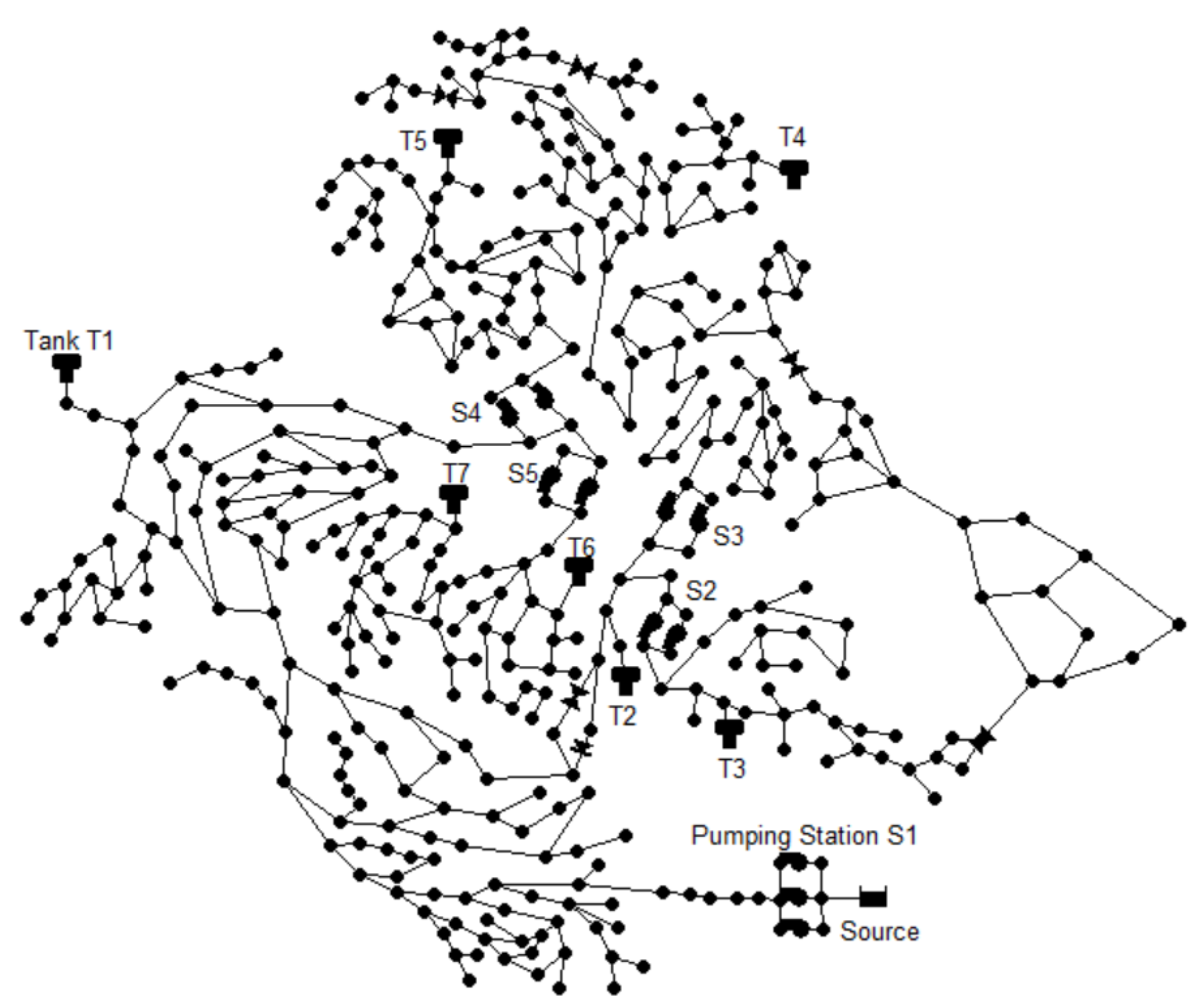
https://engineering.exeter.ac.uk/research/cws/resources/benchmarks/, accessed on 8 May 2023). The D-town hydraulic model consists of 399 junctions, 7 storage tanks, 443 pipes and 11 pumps divided into 5 pumping stations. The schema of the D-town network is presented in
Figure 1.
The training dataset was generated by performing several EPANET simulations and collecting information on the elements of the network at each time step utilizing EPANET TOOLS 1.0.0, a package enabling the user to call all the EPANET programmer’s toolkit functions within Python scripts. For each simulation, the input file was modified to simulate different water demands for each node and different initial states for tanks and pumps, leading to a different efficiency and quality of the service. The resulting dataset is a collection of 67K samples representing different network states. As described in
Section 3.1, each sample was labeled with
,
and
according to its efficiency (
) and quality (
) indicator. In particular, the efficiency indicator was computed by quantifying the energy consumed by pumping stations and the quality indicator was computed by observing whether the pressure of each node is in its optimal pressure range or measuring how much lower it is than its lower limit or greater it is than its higher extreme. More specifically, if the constraint violation for a pattern is greater than the median constraint violation in the training set, its output is set to
. If it is lower but the energy efficiency for the pattern is worse than the median energy efficiency in the training set, its output is set to
. Finally, if both indicators are better than the median, the output is set to
. Afterwards, a three-fold cross-validation procedure was used to select the optimal LLM parameters for generating the rule-based model. The parameter set leading to the higher average Cohen’s K in the validations sets was used to extract rules predicting the output value based on the level of the tanks and the number of active pumps in each pumping station.
To enhance the robustness of the evaluation, a separate set (named test set) of simulated patterns was generated, and will be used for evaluation and comparison. In other words, RBC was applied, on top of the rules generated by the LLM in the training step, to drive the controls of the system (i.e., to turn on/off some pumps) in such a way that the QoS (firstly) and the efficiency (secondly) of the network are improved. The model trained by the LLM obtains an accuracy of and a Cohen’s K of 0.76 on the test set.
The QoS and efficiency measured after the control actions provided by the RBC approach were compared with the same indicators in two different scenarios. Firstly, the system indicators after applying RBC controls were compared with the system indicators if no actions had been taken. We will refer to this as the no action case. In the second scenario, RBC was compared with one of the most used control approach, where suggestions were generated by applying the genetic algorithm. The used genetic representation is the binary one, where each gene is a pump status; the fitness is a combination of efficiency and quality indicators, where their weight parameters were set in order to favor the former one; the selection method is the proportional selection; the crossover method is the single-point crossover with a probability equal to 0.9 and a mutation probability equal to 0.1. The population size was set to 100; the best solution was maintained without any change in each generation; and the termination conditions were: 40 generations were explored; 5 steps were performed without improving the best solution.
In all cases, the system indicators were evaluated by the EPANET simulator 15 min after the controls application.
It is noteworthy that the RBC approach only needs a pre-training rule-based model to generate the control suggestions. The genetic algorithms procedure, on the other hand, requires hydraulic simulations to compute the fitness used to select the best suggestions. For this reason, genetic algorithms can be used only after the formulation of a physical model representing, with some degree of approximation, the functioning of the water distribution network.
To set up the comparison, EPANET was used as a support for genetic algorithms. All the comparisons were made using 30K samples that are different from the training set but generated with the same approach. Each sample was given as an input to the control method and the effect of the control output was checked 15 min after the application through EPANET simulations. EPANET allows us to insert a demand profile as a factor that is multiplied by a standard water demand value. Since EPANET was used both to select and to evaluate the solution generated by the genetic algorithms, Gaussian noise with an average equal to zero and standard deviation equal to 0.05 was added to the EPANET multiplier of the water demand in order to also take into account the approximation that characterizes the physical model of the system. To avoid excessive variances, the expected water demand profile used for GA optimization was simulated to differ at most from the real demand.
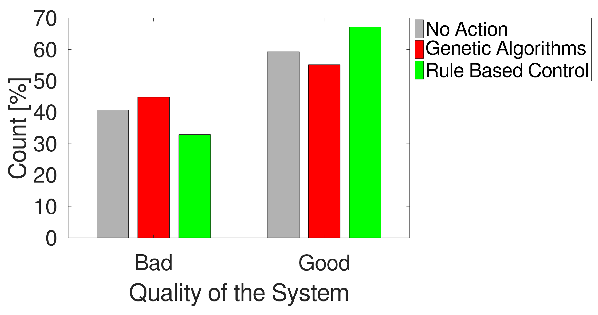
The first comparison regards the different behaviors in terms of QoS. As shown in
Figure 2, when RBC is applied, the occurrence of the
output in the next 15 min is avoided in
of cases. If no action is applied, the
is avoided in
of cases, whereas only
of patterns prevent the
output if genetic algorithms are applied.
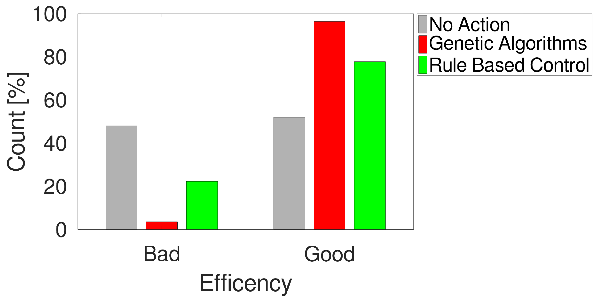
Figure 3 reports the results of experiments when considering energy efficiency and puts the QoS in a broader perspective. As illustrated, genetic algorithms result in an improved level of consumption compared to the median in
of cases. If no controls are applied, this only happens in
of cases, whereas the RBC approach achieves
of good cases if energy efficiency alone is considered.
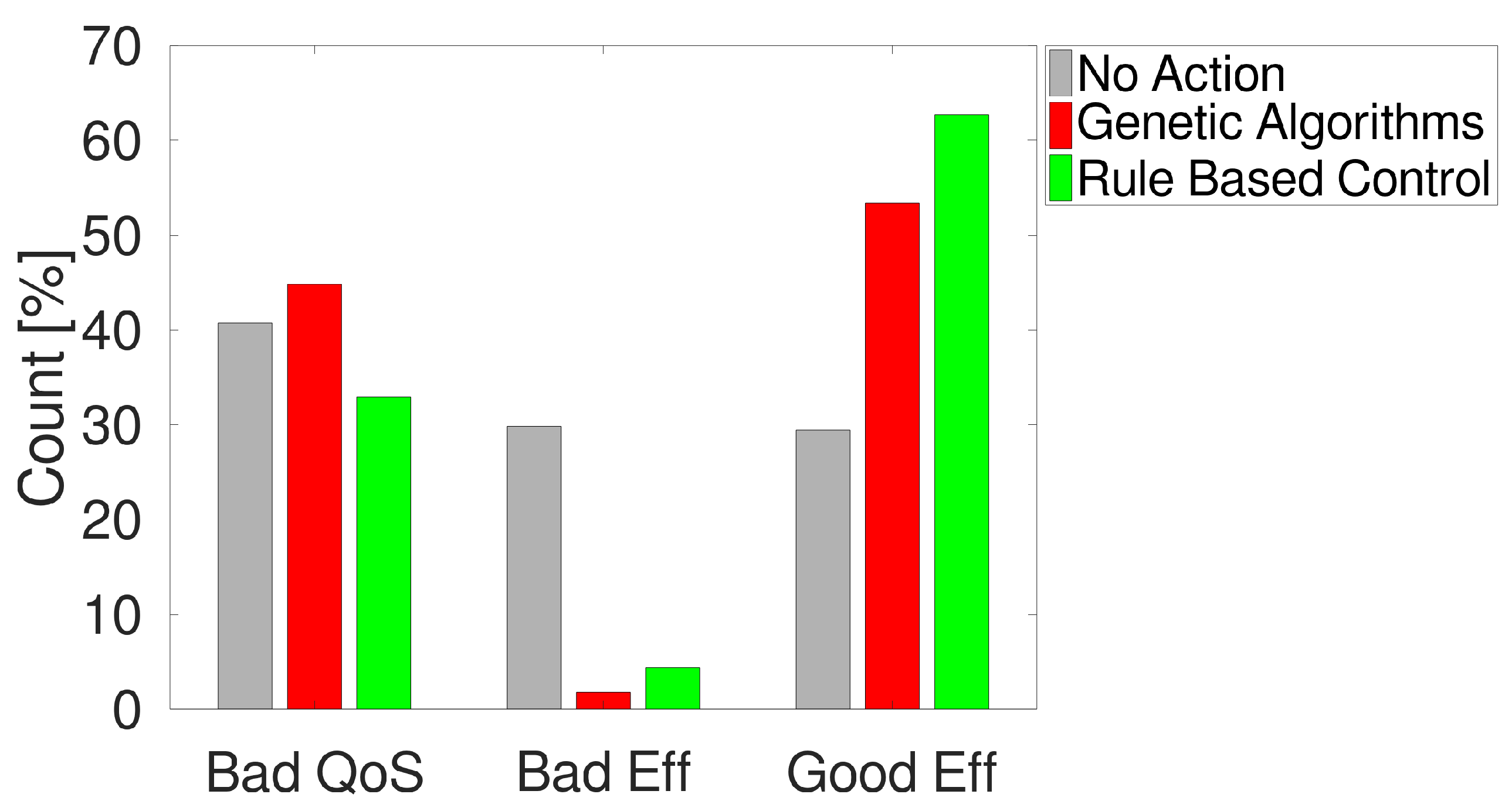
Combining the two elements, it is possible to see (in
Figure 4) that, referring to the
,
and
possible output values, RBC obtains the lowest percentage of cases in the worst class (
) and the highest percentage of cases in the best class (
).
Table 1 resumes the output distribution in the three cases.
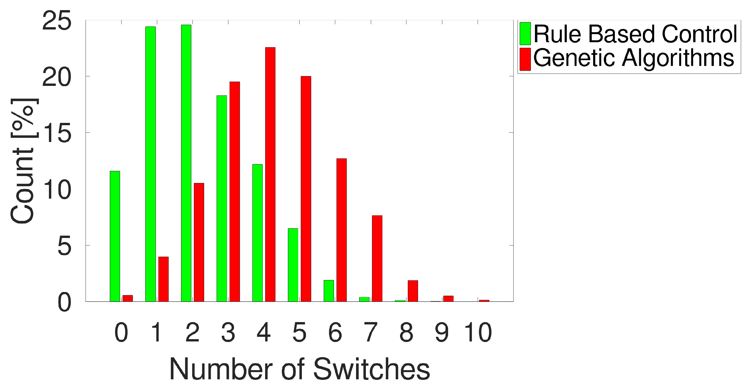
It is also worth considering that turning pumps on and off at a high rate in such a complex and critical system as a water main may not be desirable for stability reasons. To take this aspect into account,
Figure 5 shows a comparison in terms of the average number of changes that are suggested to improve the performance. In this case, only RBC and GA can be compared because, in the no action case, by definition, the number of changes is 0. From the histogram, it can be seen that more than 60% of cases RBC suggest 0, 1 or 2 switches, while the frequency of a higher number of switches decreases quickly.
On the contrary, in more than 60% of cases, GAs propose more than 3 changes, almost never suggest 0 changes and suggest 1 switch in less than 5% of cases. The average number of changes per iteration for RBC is , compared to for GAs. This means that, considering all the set of pumps during one day (i.e., 96 iterations of the control algorithm since it runs every 15 min), approximately 216 switches are expected for RBC whereas, on average, GAs suggest 407 switches.
As far as the computation time is concerned, on average, RBC requires s for a single run, whereas a single run for the GAs requires 56 s.
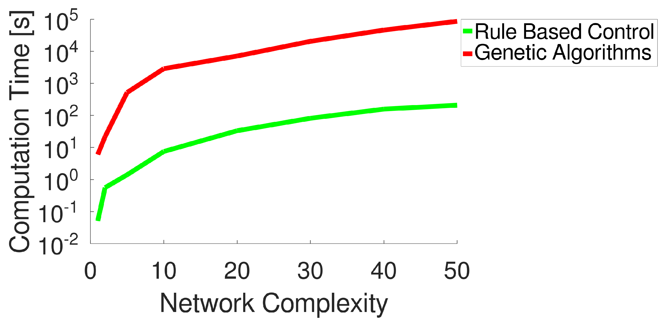
The time needed for computation depends on the complexity of the network to be controlled. For this reason, the behavior of time needed for computation as a function of the complexity of the network (measured as the ratio of the number of nodes with respect to the original network) is shown in
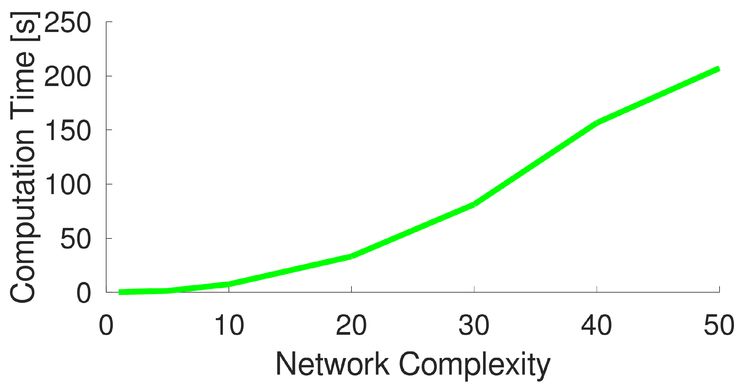
Figure 6. From this plot, it is evident that RBC is able to perform far quicker than GAs, even when the complexity of the network increases. This is not surprising as the model used by RBC is much more simple than the hydraulic simulator used by GAs. To better evaluate the time performance of RBC, we also plotted the time needed by the novel approach separately in
Figure 7. For example, it takes less than 50 s to optimize a network that is 20 times more complex than the original with approximately 8000 demand nodes. This also allows for application where new control rules should be generated with a high frequency. Moreover, opposite to other approaches (such as linear programming or genetic algorithms), RBC allows us to (sub)optimize the network by also considering a portion of it, thus reducing the computational burden further.
Computational efficiency, combined with the fact that RBC does not require a mathematical model of the network, makes it particularly well-suited for a reactive, on-line control application.


