
The Effects of Individuals’ Opinion and Non-Opinion Characteristics on the Organization of Influence Networks in the Online Domain


Abstract
1. Introduction
2. Literature
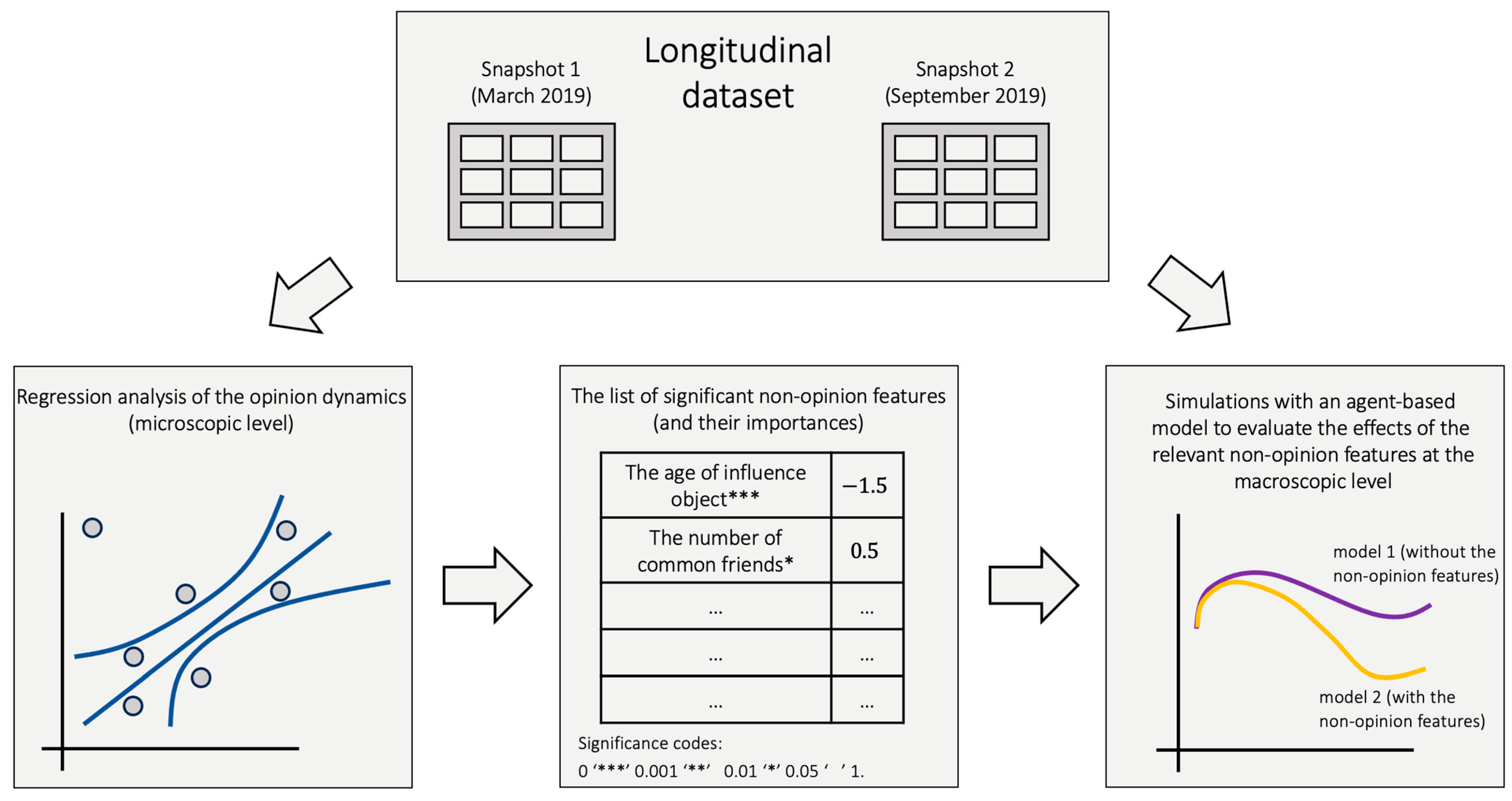
3. Overview of Our Analysis
4. Data
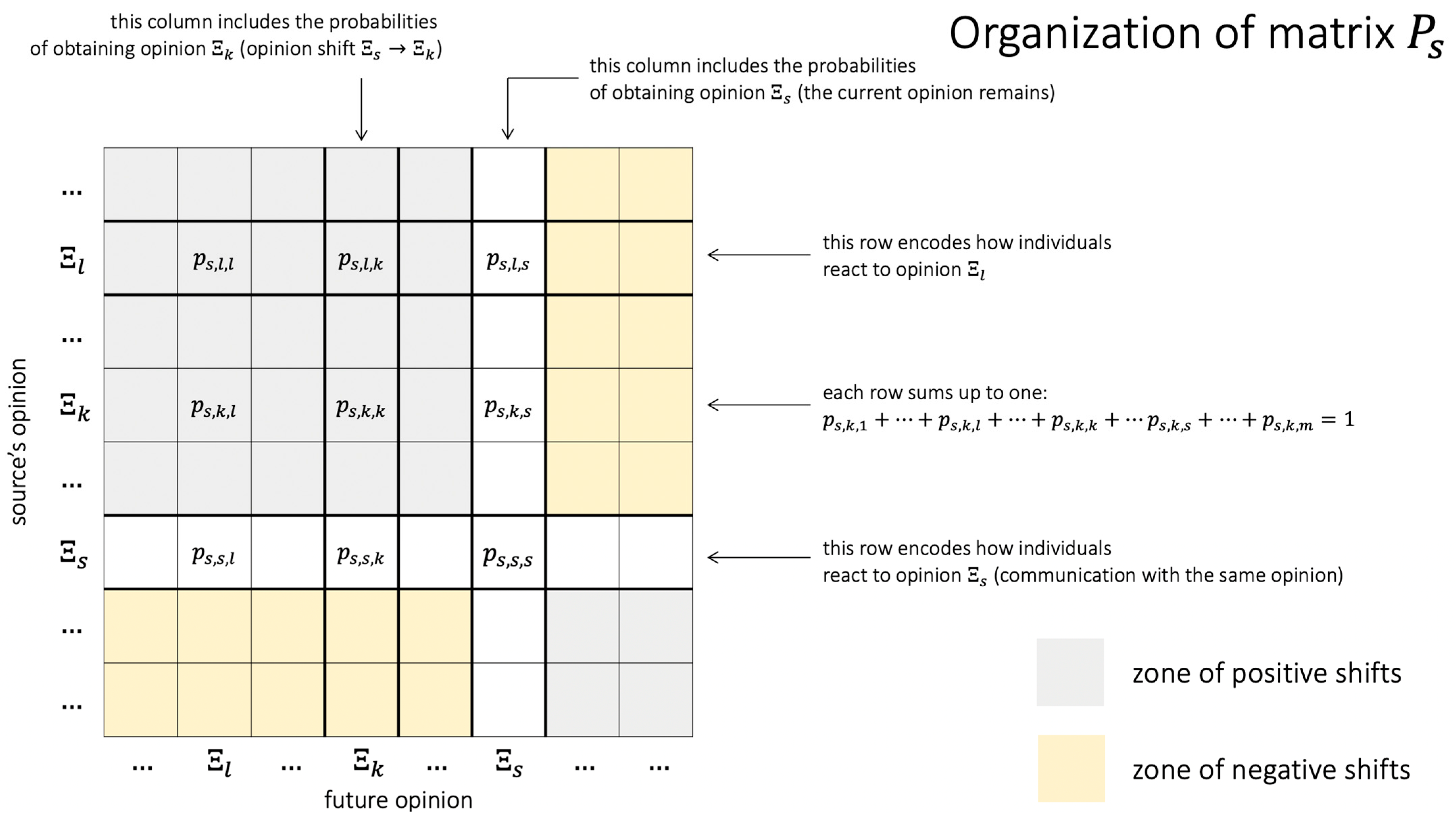
5. Notations and Terminology
6. Analysis of Opinion Dynamics
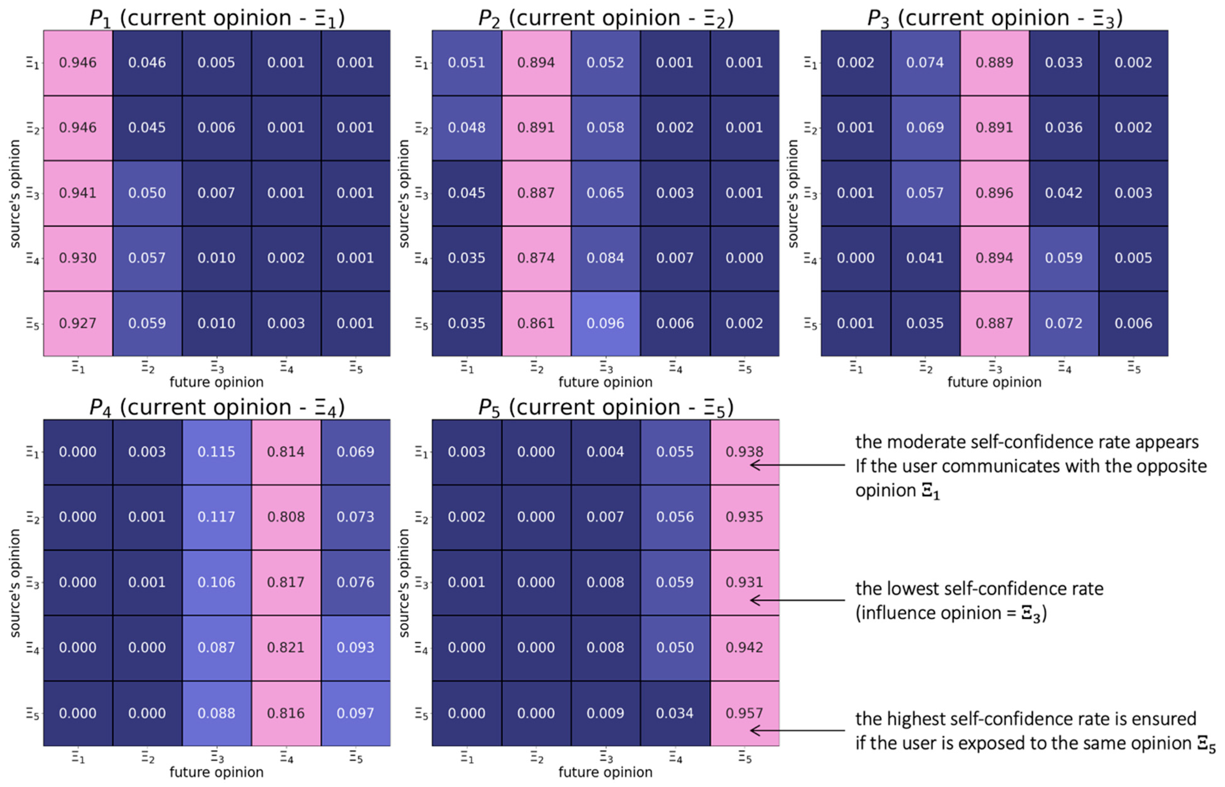
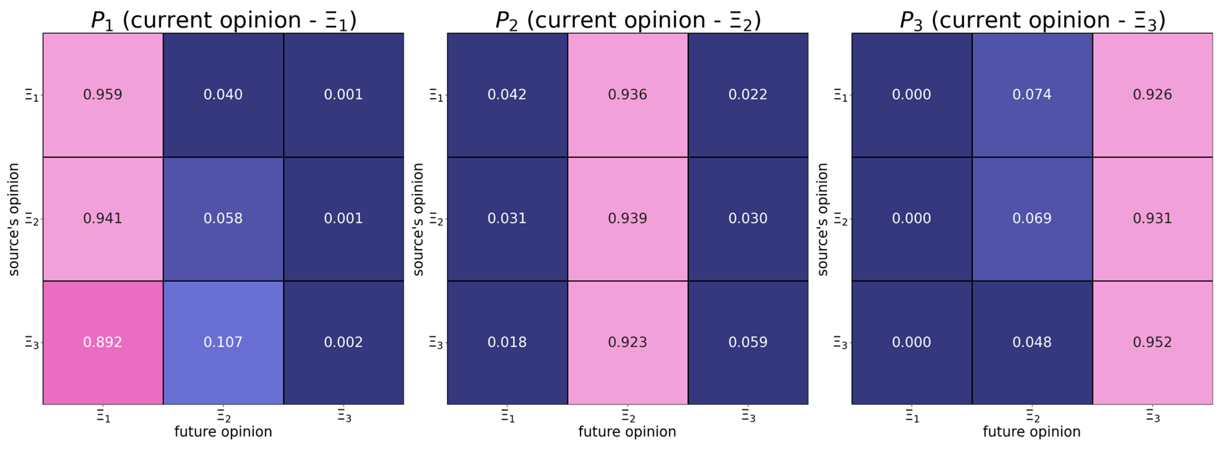
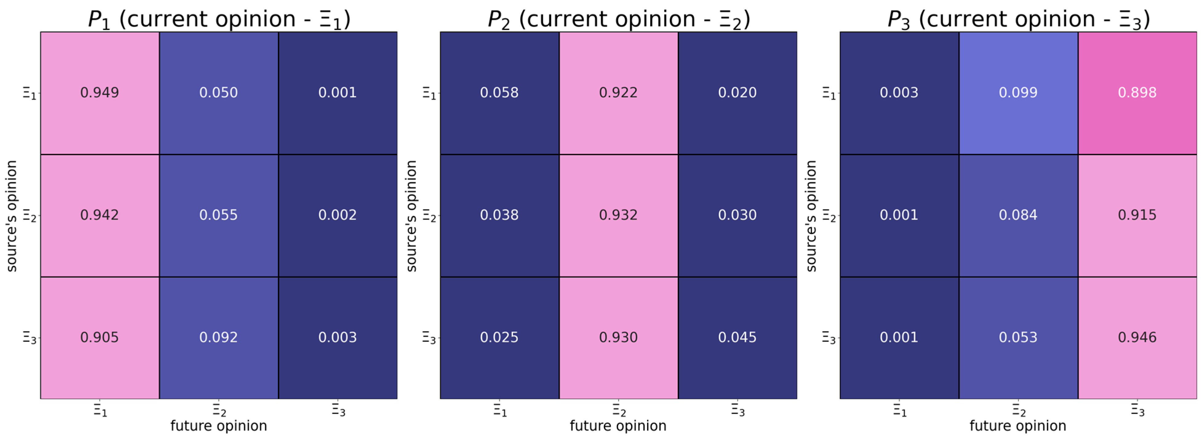
6.1. Map of Opinion Shifts
- -
- Individuals change their positions relatively rarely.
- -
- Users with radical positions are more stubborn.
- -
- Both positive and negative opinion shifts can happen, but positive shifts occur more often.
- -
- Positive shifts tend to feature the assimilative influence mechanism, whereby more distant opinions induce positive responses with larger probabilities.
- -
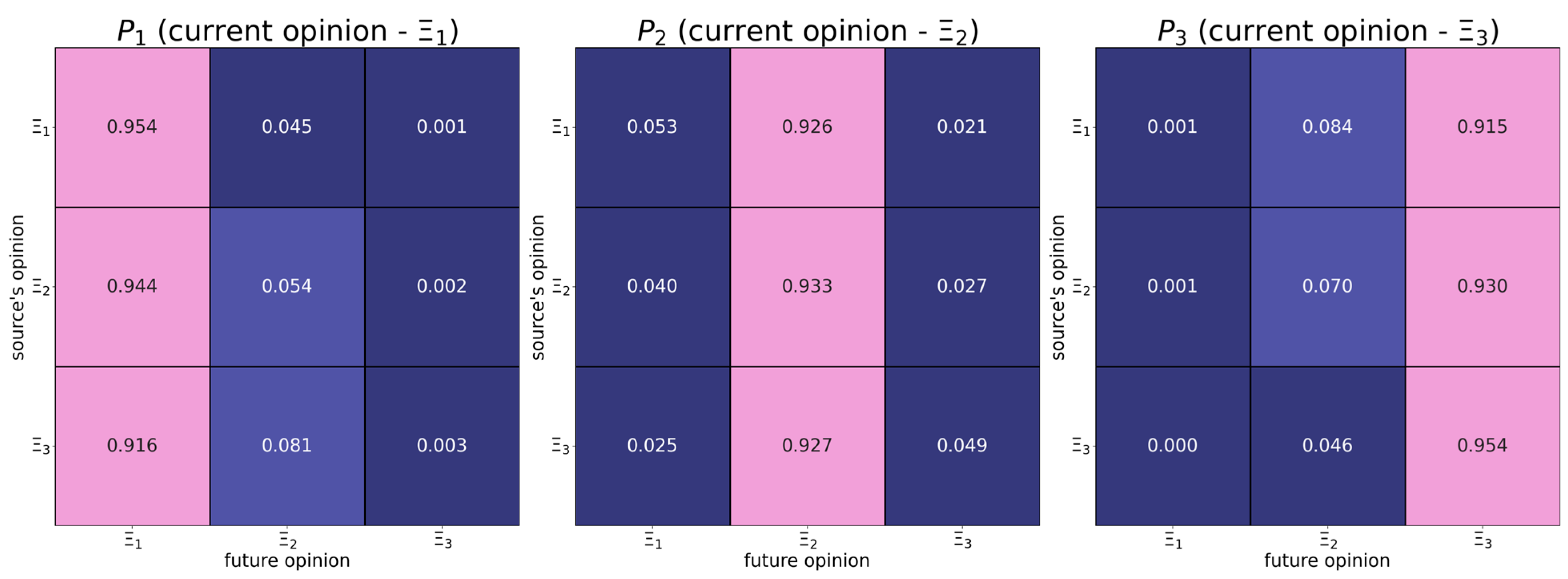
- Individuals with the right radical opinion (see the matrix in Figure 1) display a tendency to distrust too distant opinions (also known as moderated bounded confidence).
6.2. Effects of Non-Opinion Characteristics on Opinion Shifts
- -
- (the tie should remain unchanged).
- -
- (the number of common friends should be constant as it could have an effect on opinion dynamics).
- -
- (the influence source’s opinion should not undergo significant changes during the observation period—otherwise, we cannot precisely locate its value). (In fact, if in a pair of connected vertices , one vertex (say, ) has changed its opinion for more than 0.05, then the inverse pair will not appear in the corpus of observations. Further, if both the vertices have substantially modified their opinions, then the tie is completely ignored).
7. Simulations
7.1. Motivation
7.2. Agent-Based Models
7.3. Simulation Design
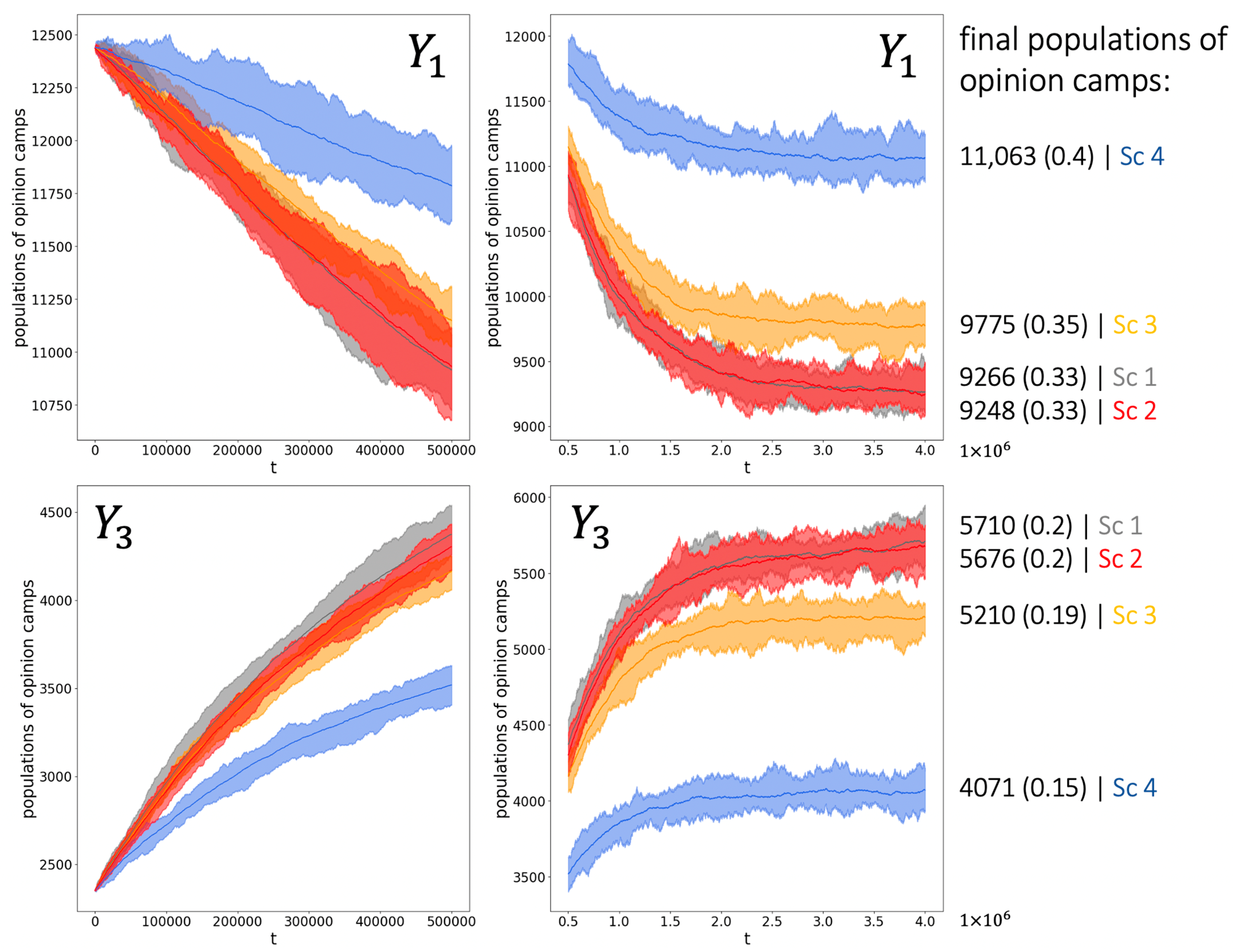
7.4. Results
8. Discussion and Conclusions
Author Contributions
Funding
Data Availability Statement
Acknowledgments
Conflicts of Interest
Appendix A
- -
- (the focal tie should remain unchanged).
- -
- (the number of common friends should be constant as it could have an effect on opinion dynamics).
- -
- (the influence source’s opinion should not undergo significant changes during the observation period—otherwise, we cannot precisely locate its value).
Appendix B


Appendix C

References
- Flache, A.; Mäs, M.; Feliciani, T.; Chattoe-Brown, E.; Deffuant, G.; Huet, S.; Lorenz, J. Models of Social Influence: Towards the Next Frontiers. J. Artif. Soc. Soc. Simul. 2017, 20. [Google Scholar] [CrossRef]
- Proskurnikov, A.V.; Tempo, R. A tutorial on modeling and analysis of dynamic social networks. Part I. Annu. Rev. Control 2017, 43, 65–79. [Google Scholar] [CrossRef]
- Friedkin, N.E.; Proskurnikov, A.V.; Bullo, F. Group dynamics on multidimensional object threat appraisals. Soc. Netw. 2021, 65, 157–167. [Google Scholar] [CrossRef]
- Friedkin, N.E.; Bullo, F. How truth wins in opinion dynamics along issue sequences. Proc. Natl. Acad. Sci. USA 2017, 114, 11380–11385. [Google Scholar] [CrossRef]
- Carpentras, D.; Maher, P.J.; O’Reilly, C.; Quayle, M. Deriving an Opinion Dynamics Model from Experimental Data. J. Artif. Soc. Soc. Simul. 2022, 25. [Google Scholar] [CrossRef]
- Clemm von Hohenberg, B.; Maes, M.; Pradelski, B. Micro Influence and Macro Dynamics of Opinion Formation (SSRN Scholarly Paper ID 2974413). Soc. Sci. Res. Netw. 2017. Available online: https://drive.google.com/file/d/1V11jIMqPIkfxmzin0jn_msiThtZtWrWe/view (accessed on 8 May 2023).
- Liu, C.C.; Srivastava, S.B. Pulling Closer and Moving Apart: Interaction, Identity, and Influence in the U.S. Senate, 1973 to 2009. Am. Sociol. Rev. 2015, 80, 192–217. [Google Scholar] [CrossRef]
- Moussaïd, M.; Kaemmer, J.E.; Analytis, P.P.; Neth, H. Social Influence and the Collective Dynamics of Opinion Formation. PLoS ONE 2013, 8, e78433. [Google Scholar] [CrossRef]
- Pansanella, V.; Morini, V.; Squartini, T.; Rossetti, G. Change my Mind: Data Driven Estimate of Open-Mindedness from Political Discussions. arXiv 2022, arXiv:2209.10470. [Google Scholar]
- Takács, K.; Flache, A.; Mäs, M. Discrepancy and Disliking Do Not Induce Negative Opinion Shifts. PLoS ONE 2016, 11, e0157948. [Google Scholar] [CrossRef]
- Barbera, P. Birds of the Same Feather Tweet Together: Bayesian Ideal Point Estimation Using Twitter Data. Political Anal. 2015, 23, 76–91. [Google Scholar] [CrossRef]
- Barberá, P. How Social Media Reduces Mass Political Polarization. Evidence from Germany, Spain, and the US; Job Market Paper; New York University: New York, NY, USA, 2014; p. 46. [Google Scholar]
- Bond, R.M.; Fariss, C.J.; Jones, J.J.; Kramer, A.D.I.; Marlow, C.; Settle, J.E.; Fowler, J.H. A 61-million-person experiment in social influence and political mobilization. Nature 2012, 489, 295–298. [Google Scholar] [CrossRef] [PubMed]
- Corradini, E.; Nocera, A.; Ursino, D.; Virgili, L. Investigating negative reviews and detecting negative influencers in Yelp through a multi-dimensional social network based model. Int. J. Inf. Manag. 2021, 60, 102377. [Google Scholar] [CrossRef]
- Kozitsin, I.V. Formal models of opinion formation and their application to real data: Evidence from online social networks. J. Math. Sociol. 2020, 46, 120–147. [Google Scholar] [CrossRef]
- Kozitsin, I.V. Opinion dynamics of online social network users: A micro-level analysis. J. Math. Sociol. 2021, 47, 1–41. [Google Scholar] [CrossRef]
- Stöckli, S.; Hofer, D. Susceptibility to social influence predicts behavior on Facebook. PLoS ONE 2020, 15, e0229337. [Google Scholar] [CrossRef]
- Xiong, F.; Liu, Y.; Cheng, J. Modeling and predicting opinion formation with trust propagation in online social networks. Commun. Nonlinear Sci. Numer. Simul. 2017, 44, 513–524. [Google Scholar] [CrossRef]
- Bonifazi, G.; Cauteruccio, F.; Corradini, E.; Marchetti, M.; Pierini, A.; Terracina, G.; Ursino, D.; Virgili, L. An approach to detect backbones of information diffusers among different communities of a social platform. Data Knowl. Eng. 2022, 140, 102048. [Google Scholar] [CrossRef]
- DeGroot, M.H. Reaching a consensus. J. Am. Stat. Assoc. 1974, 69, 118–121. [Google Scholar] [CrossRef]
- Friedkin, N.E.; Proskurnikov, A.V.; Tempo, R.; Parsegov, S.E. Network science on belief system dynamics under logic constraints. Science 2016, 354, 321–326. [Google Scholar] [CrossRef]
- Ravazzi, C.; Dabbene, F.; Lagoa, C.; Proskurnikov, A.V. Learning Hidden Influences in Large-Scale Dynamical Social Networks: A Data-Driven Sparsity-Based Approach, in Memory of Roberto Tempo. IEEE Control Syst. 2021, 41, 61–103. [Google Scholar] [CrossRef]
- Sears, D.O. College sophomores in the laboratory: Influences of a narrow data base on social psychology’s view of human nature. J. Pers. Soc. Psychol. 1986, 51, 515–530. [Google Scholar] [CrossRef]
- Peshkovskaya, A.; Myagkov, M.; Babkina, T.; Lukinova, E. Do women socialize better? Evidence from a study on sociality effects on gender differences in cooperative behavior. CEUR Workshop Proceeding 2017, 1968, 41–51. [Google Scholar]
- Peshkovskaya, A.; Babkina, T.; Myagkov, M. Social context reveals gender differences in cooperative behavior. J. Bioecon. 2018, 20, 213–225. [Google Scholar] [CrossRef]
- Peshkovskaya, A.; Babkina, T.; Myagkov, M. In-group cooperation and gender: Evidence from an interdisciplinary study. In Global Economics and Management: Transition to Economy 4.0; Kaz, M., Ilina, T., Medvedev, G.A., Eds.; Springer International Publishing: Cham, Switzerland, 2019; pp. 193–200. [Google Scholar] [CrossRef]
- Eagly, A.H. Gender and social influence: A social psychological analysis. Am. Psychol. 1983, 38, 971–981. [Google Scholar] [CrossRef]
- Kozitsin, I.V.; Gubanov, A.V.; Sayfulin, E.R.; Goiko, V.L. A nontrivial interplay between triadic closure, preferential, and anti-preferential attachment: New insights from online data. Online Soc. Netw. Media 2023, 34, 100248. [Google Scholar] [CrossRef]
- Deffuant, G.; Neau, D.; Amblard, F.; Weisbuch, G. Mixing beliefs among interacting agents. Adv. Complex Syst. 2000, 3, 87–98. [Google Scholar] [CrossRef]
- Hegselmann, R.; Krause, U. Opinion dynamics and bounded confidence models, analysis, and simulation. J. Artif. Soc. Soc. Simul. 2002, 5, 1–33. [Google Scholar]
- Kurahashi-Nakamura, T.; Mäs, M.; Lorenz, J. Robust Clustering in Generalized Bounded Confidence Models. J. Artif. Soc. Soc. Simul. 2016, 19. [Google Scholar] [CrossRef]
- Balietti, S.; Getoor, L.; Goldstein, D.G.; Watts, D.J. Reducing opinion polarization: Effects of exposure to similar people with differing political views. Proc. Natl. Acad. Sci. USA 2021, 118, e2112552118. [Google Scholar] [CrossRef]
- Aral, S.; Walker, D. Tie Strength, Embeddedness, and Social Influence: A Large-Scale Networked Experiment. Manag. Sci. 2014, 60, 1352–1370. [Google Scholar] [CrossRef]
- Friedkin, N.E. A Formal Theory of Reflected Appraisals in the Evolution of Power. Adm. Sci. Q. 2011, 56, 501–529. [Google Scholar] [CrossRef]
- Kozitsin, I.V.; Chkhartishvili, A.; Marchenko, A.M.; Norkin, D.O.; Osipov, S.D.; Uteshev, I.; Goiko, V.L.; Palkin, R.V.; Myagkov, M.G. Modeling Political Preferences of Russian Users Exemplified by the Social Network Vkontakte. Math. Model. Comput. Simul. 2020, 12, 185–194. [Google Scholar] [CrossRef]
- Clifford, P.; Sudbury, A. A model for spatial conflict. Biometrika 1973, 60, 581–588. [Google Scholar] [CrossRef]
- Mäs, M.; Flache, A. Differentiation without Distancing. Explaining Bi-Polarization of Opinions without Negative Influence. PLoS ONE 2013, 8, e74516. [Google Scholar] [CrossRef] [PubMed]
- Kozitsin, I.V. A general framework to link theory and empirics in opinion formation models. Sci. Rep. 2022, 12, 5543. [Google Scholar] [CrossRef]
- Petrov, A.; Akhremenko, A.; Zheglov, S. Dual Identity in Repressive Contexts: An Agent-Based Model of Protest Dynamics. Soc. Sci. Comput. Rev. 2023. [Google Scholar] [CrossRef]
- Preoţiuc-Pietro, D.; Liu, Y.; Hopkins, D.; Ungar, L. Beyond binary labels: Political ideology prediction of twitter users. In Proceedings of the 55th Annual Meeting of the Association for Computational Linguistics, Vancouver, BC, Canada, 30 July–4 August 2017; pp. 729–740. [Google Scholar] [CrossRef]


| Independent Variable | Definition | Hypothesis |
|---|---|---|
| The absolute difference in opinions | should have a positive effect on the dependent variable—from Figure 3 it follows that more distant opinions tend to be more attractive. | |
| The absolute difference in age | should have a negative effect on the dependent variable—a non-opinion similarity stimulates the decrease in opinion discrepancies [32]. | |
| This variable demonstrates if two users have different genders () or not () | should have a negative effect on the dependent variable—a non-opinion similarity stimulates the decrease in opinion discrepancies [32]. | |
| The nodal degree of the influence object | may have a negative effect on the dependent variable—we hypothesize that individuals that have many friends should perceive themselves as more valuable and having a higher social status and thus should be more attached to their own views [27]. | |
| The number of common friends | should have a positive effect on the dependent variable—strong ties are more effective in conducting social influence [33]. | |
| The opinion of the influence object | should have a negative effect on the dependent variable—from Figure 3, it follows that users whose opinions are close to the right endpoint of the opinion spectrum are more stubborn. | |
| This dummy variable shows if the gender of is female | should have a positive effect on the dependent variable—according to Refs. [24,25,26], females cooperate better than males. | |
| The age of | This covariate should have a negative effect on the dependent variable—younger individuals tend to be more sensitive to influence [23]. |
| 2.508 | 1.857 | 1.448 | 1.874 | 1.483 | 3.432 | 1.901 | 5.346 |
| 2.247 | 1.556 | 1.422 | 1.853 | 1.45 | 2.948 | 1.701 | – |
| Coefficient | Std Error | t | P > |t| | |
|---|---|---|---|---|
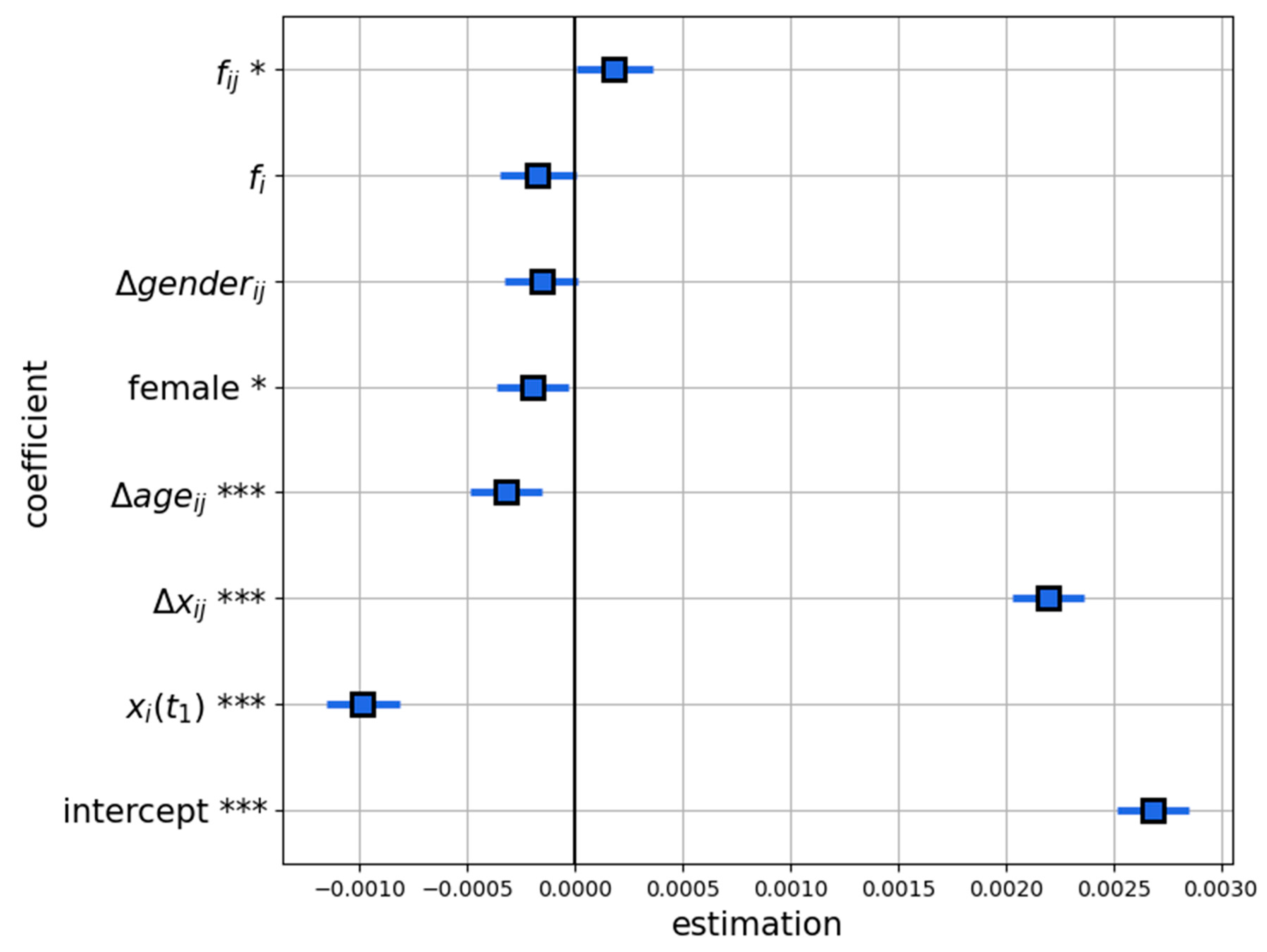
| Intercept | 0.0027 | 8.53 × 10⁻⁵ | 31.467 | 0.000 *** |
| 0.0022 | 8.63 × 10⁻⁵ | 25.451 | 0.000 *** | |
| −0.0003 | 8.6 × 10⁻⁵ | −3.724 | 0.000 *** | |
| −0.0002 | 8.57 × 10⁻⁵ | −1.826 | 0.068 | |
| −0.0002 | 9.06 × 10⁻⁵ | −1.911 | 0.056 | |
| 0.0002 | 9.01 × 10⁻⁵ | 2.018 | 0.044 * | |
| −0.001 | 8.71 × 10⁻⁵ | −11.329 | 0.000 *** | |
| −0.0002 | 8.67 × 10⁻⁵ | −2.276 | 0.023 * |
| Types of Pairs | The Values of the Variable | ||
|---|---|---|---|
| Type 1 | |||
| Type 2 | |||
| Type 3 | |||
| Type 4 | |||
| Type 5 | |||
| Type 6 | |||
| Type 7 | |||
| Type 8 | |||
| Agents’ Characteristics Used in Simulations | Random Shuffle of Nodes | ||
|---|---|---|---|
| Opinion | Non-Opinion Characteristics | ||
| Scenario 1 | + | − | − |
| Scenario 2 | + | − | + |
| Scenario 3 | + | + | − |
| Scenario 4 | + | + | + |
Disclaimer/Publisher’s Note: The statements, opinions and data contained in all publications are solely those of the individual author(s) and contributor(s) and not of MDPI and/or the editor(s). MDPI and/or the editor(s) disclaim responsibility for any injury to people or property resulting from any ideas, methods, instructions or products referred to in the content. |
© 2023 by the authors. Licensee MDPI, Basel, Switzerland. This article is an open access article distributed under the terms and conditions of the Creative Commons Attribution (CC BY) license (https://creativecommons.org/licenses/by/4.0/).
Share and Cite
Gezha, V.N.; Kozitsin, I.V. The Effects of Individuals’ Opinion and Non-Opinion Characteristics on the Organization of Influence Networks in the Online Domain. Computers 2023, 12, 116. https://doi.org/10.3390/computers12060116
Gezha VN, Kozitsin IV. The Effects of Individuals’ Opinion and Non-Opinion Characteristics on the Organization of Influence Networks in the Online Domain. Computers. 2023; 12(6):116. https://doi.org/10.3390/computers12060116
Chicago/Turabian StyleGezha, Vladislav N., and Ivan V. Kozitsin. 2023. "The Effects of Individuals’ Opinion and Non-Opinion Characteristics on the Organization of Influence Networks in the Online Domain" Computers 12, no. 6: 116. https://doi.org/10.3390/computers12060116
APA StyleGezha, V. N., & Kozitsin, I. V. (2023). The Effects of Individuals’ Opinion and Non-Opinion Characteristics on the Organization of Influence Networks in the Online Domain. Computers, 12(6), 116. https://doi.org/10.3390/computers12060116