Image Denoising by Deep Convolution Based on Sparse Representation

Abstract

Noise filtering is a crucial task in digital image processing, performing the function of preprocessing. In this paper, we propose an algorithm that employs deep convolution and soft thresholding iterative algorithms to extract and learn the features of noisy images. The extracted features are acquired through prior and sparse representation theory for image reconstruction. Effective separation of the image and noise is achieved using an end-to-end network of dilated convolution and fully connected layers. Several experiments were performed on public images subject to various levels of Gaussian noise, in order to evaluate the effectiveness of the proposed approach. The results indicated that our algorithm achieved a high peak signal-to-noise ratio (PSNR) and significantly improved the visual effects of the images. Our study supports the effectiveness of our approach and substantiates its potential to be applied to a broad spectrum of image processing tasks.

1. Introduction

Digital image devices have a diverse range of applications, such as human recognition [1] and remote sensing [2]. During transmission and compression processes, noise is generated from latent observations that are unknown.

The focus of this paper is the classic image denoising problem. Specifically, the goal is to denoise the measurement of an ideal image X, which has been corrupted by the addition zero-mean white and homogeneous Gaussian noise, V, with a standard deviation of $\delta$. The measured image Y can be represented mathematically by the following equation:

$$Y=X+V.$$

(1)

and our objective is to recover X from Y by knowing the parameter $\delta$.

Image denoising is a crucial preprocessing step in low-level vision tasks, since noise corruption is often unavoidable during image acquisition. Demonstrably, this is a subtask within resolving an assortment of image reconstruction problems [3], such as super-resolution [4] and image restoration [5] problems, among others. VS Unni et al. [6] introduced a novel framework for image restoration that integrates linearized alternating direction method of multipliers (ADMM) and fast nonlocal denoising algorithms. The main objective of this method is to offer a computationally efficient solution for plug-and-play image restoration, which refers to utilizing pretrained denoisers within a general optimization framework for image restoration. Therefore, an effective image denoising algorithm could be applied to various image reconstruction problems. This explains why numerous researchers have proposed and improved denoising algorithms in the field of denoising in recent years.

Recently, there has been a plethora of sparse representation-based approaches suggested for image denoising. The K-SVD algorithm, introduced by Elad and Aharon in 2006 [7], was among the earliest sparse representation-based approaches. The K-SVD algorithm is a dictionary learning method that yields a dictionary of atoms that grasps the structural properties of natural images. By representing the noisy image as a linear combination of atoms learned from the dictionary, the K-SVD algorithm denoises the image by thresholding the coefficients. In 2007, another popular sparse representation-based approach named the BM3D algorithm was proposed by Dabov et al. [8]. The BM3D algorithm, which is a block-matching and 3D-filtering technique, makes use of the 3D redundancy existing in similar image patches. Initially, the BM3D algorithm groups identical patches together and employs 3D filtering on each group, to acquire an initial estimate of the denoised image. This estimate is then enhanced iteratively using a nonlocal means filter.

In recent years, various approaches based on sparse representation have been suggested for image denoising. Sun et al. [9] introduced a novel image denoising algorithm based on the sparse representation model that uses linear Bayesian maximum a posteriori (MAP) estimation. In order to solve inverse generalized image problems, an a prior probability distribution is constructed in the representation vector. This approach enables the construction of a linear Bayesian MAP estimator that adapts to the observations and acquires the most probable solution. In addition, Xu et al. [10] recommended a technique that learns a nonlocal similarity prior from images and utilizes this for denoising. A widely used approach to image denoising was suggested in [11], where the method uses the concept of linear Bayesian maximum a posteriori (MAP) estimation.

The main contribution of this paper is proposing an image denoising algorithm based on a combination of hollow convolution and the traditional KSVD algorithm. By combining the KSVD dictionary learning algorithm with deep learning, the accuracy and robustness of the denoising algorithm are improved. The experimental results show that this algorithm performed much better than BM3D, WNNM, and other algorithms in objective indicators and in subjective visual evaluation. Moreover, it can compete with DnCNN, a deep learning method with a good comprehensive performance, providing a new concept for image denoising.

The paper is structured as follows: Section 2 provides a literature review on image denoising, Section 3 outlines the proposed denoising framework, Section 4 details the simulation design and comparative analysis. The conclusion section summarizes the main contributions.

2. Related Work

Image denoising has always been a hot research topic in the field of computer vision. Over the past few decades, many signal processing and machine learning-based methods have been proposed for image denoising. Among them, sparse representation and deep learning are two popular methods. Sparse representation is a method of representing an image as a set of coefficients with respect to a basis. The basic idea is to use as few coefficients as possible to represent the original signal. In image denoising, sparse representation methods typically reduce the impact of noise by exploiting the sparseness property of the image, thus achieving good performance. Deep learning is a method of learning data representations using deep neural networks. Compared to traditional methods based on feature extraction and classifiers, deep learning has a stronger representation ability and better generalization performance. In image denoising, deep learning methods have achieved excellent performance in many scenarios. This section provides a detailed introduction and comparison of image denoising methods based on sparse representation and deep learning.

2.1. Sparse-Based

In recent decades, image denoising has become an extensively researched topic in image processing [12]. Traditionally, filter-based denoising methods dominated the field; however, machine learning methods, such as sparse methods, have gained prominence over time. One such method, the non-local centralized sparse representation (NCSR) method [13], utilizes nonlocal self-similarity to optimize sparse methods and has improved image denoising performance significantly. To minimize computational expenses, this method uses dictionary learning to quickly filter noise [14]. Prior knowledge, specifically total variation regularization, can be deployed to smooth noisy images, process damaged images, and restore detailed information from clean images [15,16]. Apart from the NCSR method, several other competitive image denoising methods exist. Examples of such methods include Markov random field (MRF) [17], weighted nuclear norm minimization (WNNM) [18], learned simultaneous sparse coding (LSSC) [19], cascaded shrinkage fields (CSF) [20], trained non-linear reaction diffusion (TNRD) [21], and gradient histogram estimation and preservation (GHEP) [22]. The fundamental principle of these methods is to exploit various techniques to extract and smooth the image features to accomplish denoising.

Various techniques have recently been proposed for overcoming noise within digital images, including the use of clustering, dictionary learning algorithms, and compressed sensing reconstruction. Khmag et al. [23] introduced a clustering-based denoising technique using a dictionary learning algorithm in the wavelet domain, which promoted the sparse and multi-resolution representation of images by utilizing second-generation wavelet clustering coefficients. In contrast, Tallapragada et al. [24] focused on denoising mixed-noise images by developing a model that combined weighted encoding and nonlocal similarity techniques. They defined a weight matrix to optimize operations at specific locations on the image, followed by the introduction of nonlocal similarity features that generated a high-quality reconstructed image. Similarly, Mahdaoui and Ouahabi [25] proposed a denoising compressed sensing regularization (DCSR) algorithm, which used total variation regularization and nonlocal self-similarity constraints. The authors optimized the algorithm using an enhanced Lagrange multiplier, which overcomes the nonlinearity and non-differentiability issues associated with the regularization term.

Despite the promising performance of these techniques, they suffer from certain limitations, such as the requirement for optimization methods during testing, manual parameter tuning, and a potential inability to capture nonlocal dependencies in images.

2.2. Deep Learning-Based Denoising

Recently, with their flexible architectures, deep learning techniques have shown the potential to overcome the aforementioned limitations. Deep learning techniques were first used for image processing in the 1980s [26]. Zhou et al. [27] applied these techniques to image denoising. The proposed denoising method uses a neural network to recover a clean latent image. The neural network has a known shift-invariant blur function and additive noise. Weighted factors are utilized to remove complex noise. To reduce computational costs, the authors propose a feed-forward network to balance the denoising efficiency and performance [28]. The feed-forward network is capable of utilizing a Kuwahara filter, which is similar to convolution, to smooth the corrupted image.

Deep networks were first applied to the denoising of digital images in 2015 [29]. These networks eliminated the need to set parameters manually to remove noise. After that, deep networks became extensively applied in various areas such as speech denoising [30], video restoration [31], and image restoration [32]. Burger et al. [33] described a patch-based denoising algorithm, where a given noisy image was divided into overlapping image patches. These patches then served as inputs to train a multilayer perceptron (MLP) with a large dataset. Thus, the network learned how to map each noisy image patch to its corresponding clean versions. This patch-based approach has been proven to deal with complex spatial correlation noise and achieve state-of-the-art results in digital image denoising. Mao et al. [34] used multiple convolutions and deconvolutions to suppress noise and recover a high-resolution image. For addressing multiple low-level tasks via a model, a denoising CNN (DnCNN) [35] consisting of convolutions, batch normalization (BN) [36], a rectified linear unit (ReLU) [37], and residual learning (RL) [38] was proposed to deal with image denoising, super-resolution imaging, and JPEG image deblocking. Shreyasi Ghose [39] proposed a deep convolutional denoising network. This network employed a DnCNN feedforward network as a pretraining model to denoise images with additive Gaussian white noise on a public dataset. Gai and Bao [40] proposed a new image denoising approach using an improved deep convolutional neural network (CNN) with perceptive loss. The authors propose a CNN-based approach that consisted of several layers, including convolutional, activation, and pooling layers. They also introduced an improved residual block structure to improve the CNN’s feature extraction capabilities. The proposed method outperformed traditional sparse representation-based denoising techniques, which require optimization techniques and manual parameter tuning.

Zhang et al. [41] proposed a principled formulation and framework by extending bicubic degradation-based deep SISR with the help of a plug-and-play framework, to handle LR images with arbitrary blur kernels. Specifically, the method utilized a new SISR degradation model, so as to take advantage of existing blind deblurring methods for blur kernel estimation.Cheng et al. [42] proposed a novel framework for image denoising(NBNet). The method involved training a network that can separate a signal and noise by learning a set of reconstruction bases in the feature space. Subsequently, image denoising is achieved by selecting a corresponding basis for the signal subspace and projecting the input into such a space. A fast and flexible denoising CNN (FFDNet) [43] used different noise levels and the noisy image patch as input to a denoising network, to improve the denoising speed and process blind denoising. Alternatively, a convolutional blind denoising network (CBDNet) [44] removed the noise from a given real noisy image using two sub-networks, one in charge of estimating the noise of the real noisy image, and the other for obtaining a latent clean image.

In recent years, the Unet network has garnered significant attention for its exceptional performance in image segmentation. Gurrola-Ramos presented a residual dense neural network (RDUNet) [45] for image denoising, using a densely connected hierarchical network. The RDUNet utilizes densely connected convolutional layers in its encoding and decoding layers, allowing the reuse of feature maps and local residual learning, to combat the vanishing gradient problem and expedite the learning process. Furthermore, Fan Jia [46] explored a more challenging scenario: how can an image-denoising network be more efficient and have fewer parameters? They proposed a novel cascading U-Net architecture with multiscale dense processing, named the Dense Dense U-Net (DDUNet). DDUNet comprises a series of techniques for improving model performance with fewer parameters, such as wavelet transform, multiscale dense processing, global feature fusion, and global residual learning.

3. Proposed Framework

This paper proposes an end-to-end network model that utilizes deep dilated convolution and a multilayer perceptron as the primary architecture. Additionally, it employs a sparse representation technique to extract deep image features. The sparse representation technique in this model is the standard in the area of compressed sensing. The adoption of sparse representation to extract features in this model deals with deep networks that tend to over-smooth image textures during image denoising.

Our design takes into consideration dilated convolution networks to effectively capture the intrinsic features of images. Dilated convolution can provide a larger receptive field than regular convolution, thereby enhancing the ability and flexibility of using image features as the network depth increases. Moreover, convolution networks have definite advantages in terms of training regularization parameters and dictionaries, which include the use of rectified linear units and pooling operations. These advantages make it highly appropriate for GPU computing, accelerating the training process and improving the denoising performance. The convolutional layer is a filter-based image processor that can fit a filter with excellent denoising performance on noisy images. This is achievable through training on a vast amount of data, consequently diminishing edge artifacts. 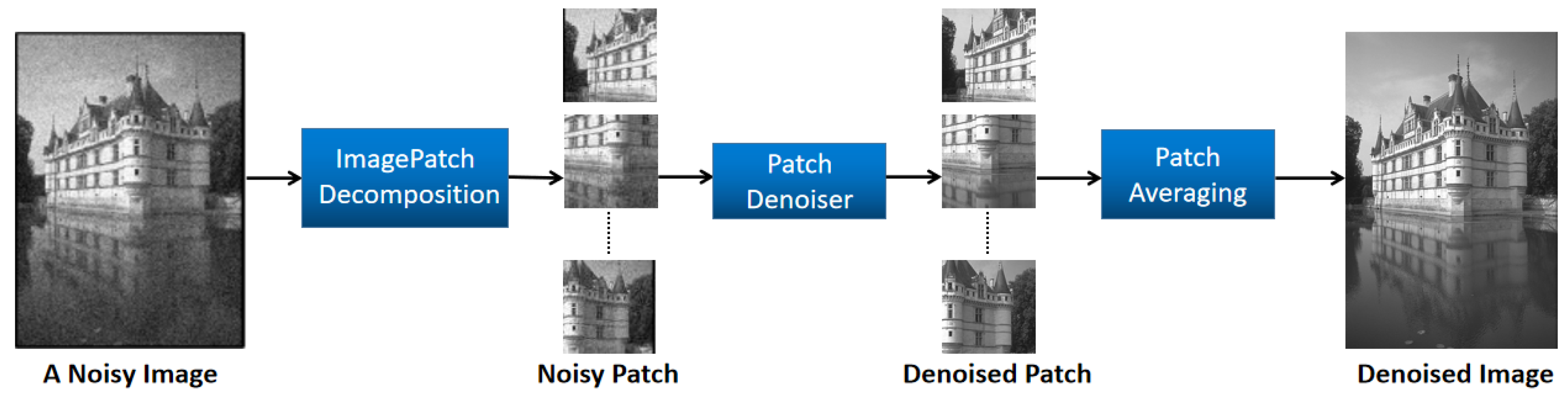Figure 1 shows that the denoising framework comprises image decomposition, patch denoiser, and patch averaging components.

Figure 1. Denoising framework.

As referenced in [33], mapping between the noisy image and the denoised image is performed on local image patches. The primary concept of this paper is to broaden local image denoising to global image denoising. This involves designing a local image Bayesian estimator along with a global image Bayesian estimator.

Since the overcomplete dictionary used here is tailored to the characteristics of the noisy input image, it is appropriate to apply dictionary learning to smaller image blocks. An image X of dimensions M × N is segmented into several fully overlapping blocks of size n × n. This approach accelerates dictionary learning, while enhancing the data processing efficiency. Moreover, the sparse nature of each block permits its local prior to be easily transformed into a global prior consistent with the Bayesian framework.

3.1. Local Prior for Image Blocks

Consider an image patch x with dimensions $n\times n$, which is reshaped by element as a column vector of length $n^2$. To effectively separate the noise from the essential features of the image, we assume the sparsity of each image block. The sparse representation of image block x can be obtained as $x=D\alpha$, where $D\in R^{n^2\times m}$, $m>>n^2$, is the DCT dictionary set tailored to x, and $\alpha \in R^m$ is a nonzero sparse vector with sparsity k, i.e., ${\parallel x\parallel }_0=k$. Given y, a noisy version of x corrupted by an additive zero-mean white Gaussian noise with standard deviation $\delta$, a maximum a posteriori (MAP) estimator can be obtained using Bayesian theory by minimizing ${\parallel \alpha \parallel }_0$ subject to $y=D\alpha$, as shown in Equation (2).

$$\widehat{\alpha }=\arg \underset{\alpha }{\min }{\parallel \alpha \parallel }_0\mathrm{s}.\mathrm{t}y=D\alpha .$$

(2)

The sparse coefficients $\alpha$ are obtained from the sparse representation of the image patch x through the dictionary D. To simplify the estimator and facilitate its solution, we replace the constraint term in Equation (2) with the difference between the noisy and the denoised image blocks. Therefore, the resulting equation is

$$\widehat{\alpha }=\arg \underset{\alpha }{\min }{\parallel \alpha \parallel }_0\mathrm{s}.\mathrm{t}{\parallel D\alpha -y\parallel }_2^2\le n^2{\delta }^2.$$

(3)

An accurate reconstruction of an ideal image can be obtained by utilizing sparse representation through an overcomplete dictionary D. The coefficient values obtained from the original image can be reconstructed exactly from the dictionary’s atoms. However, the presence of noise in the image decreases the quality of the reconstruction using the coefficients obtained from sparse representation. For controlling the sparse vector $\alpha$ and removing errors due to the standard deviation $\delta$ and noise block y, a regularization parameter $\lambda$ is utilized. The estimator problem is simplified by transforming the constraint into a penalty term to solve $\widehat{\alpha }$, and subsequently transforming the equation into its Lagrangian form.

$$\widehat{\alpha }=\arg \underset{\alpha }{\min }{\lambda \parallel \alpha \parallel }_0+\frac{1}{2}{\parallel D\alpha -y\parallel }_2^2.$$

(4)

3.2. Global Prior for Image Blocks

Sparse representation theory emphasizes the significance of sparsity in image denoising, as it automatically eliminates features that do not contain image information for noise removal. Additionally, utilizing the similarity of information between distinct image blocks in an image has been found to be advantageous for denoising, as affirmed in prior studies [37]. To highlight the synergistic nature between image blocks, it is assumed that

$$X=[x_1,x_2,\dots ,x_N]\in R^{M\times N}$$

(5)

The natural generalization of the above MAP estimator is the replacement of (4) with

$$\left\{\widehat{{\alpha }_i},\widehat{X}\right\}=\arg \underset{{\alpha }_i,X}{\min }\frac{\phi }{2}{\parallel X-Y\parallel }_2^2+\sum _i\left({\lambda }_i{∥{\alpha }_i∥}_0+\frac{1}{2}{∥D{\alpha }_i-A_{i}X∥}_2^2\right)$$

(6)

The notation $A_k$ represents the operator extracted from the image. As mentioned previously, obtaining the local prior of the image block enables a simple derivation of the global prior for the entire image X in the Bayesian framework.

The first term calculates the global logarithmic likelihood function that measures the similarity between the original image X and its noisy counterpart Y. $\phi$ represents the Lagrange multiplier, which serves as a constraint to limit the range of the first term in Equation (6). The second term is the image prior that makes sure that, in the constructed image, X, every patch $x_i=A_{i}X$ of size $n\times n$ in every location has a sparse representation with bounded error.

Given all $\widehat{{\alpha }_i}$, we can now fix these and turn to updating X. Returning to (6), we need to solve

$$\widehat{X}=\arg \underset{X}{\min }\frac{\phi }{2}{\parallel X-Y\parallel }_2^2+\frac{1}{2}\sum _i{∥D{\alpha }_i-A_{i}X∥}_2^2$$

(7)

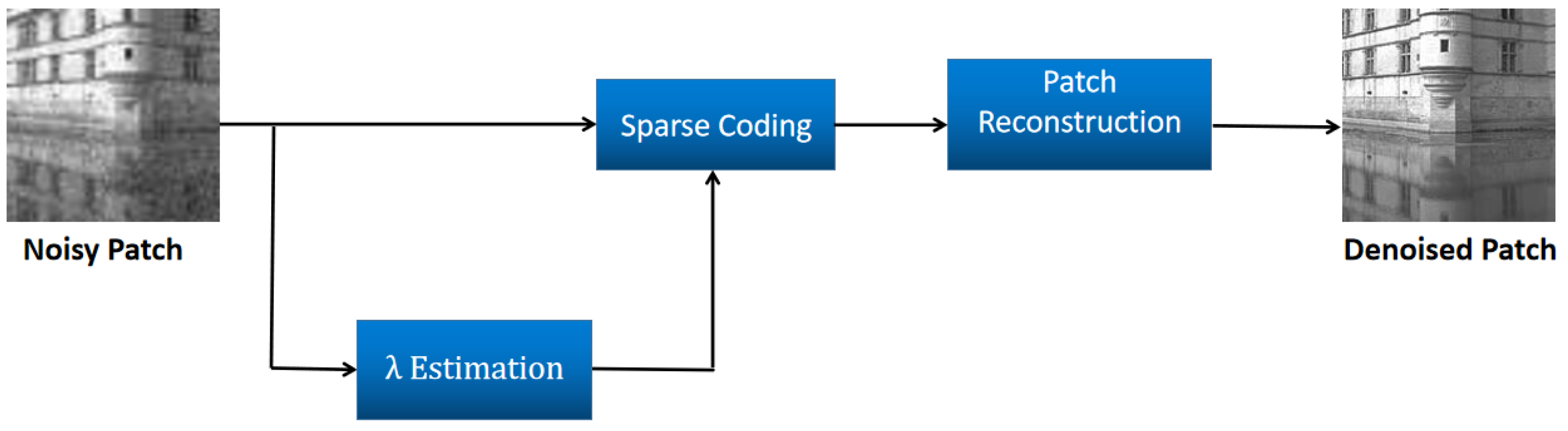
3.3. Patch Denoiser

According to Equation (7), obtaining an optimal sparse coefficient is crucial for reconstructing a high-quality, denoised image. This section is devoted to solving the image’s optimal sparse coefficient. Three steps are involved in image denoising: sparse coding, parameter estimation, and image reconstruction. Figure 2 illustrates these steps.

Figure 2. Patch denoiser.

3.3.1. Sparse Coding

Equation (4) provides the objective equation for solving the sparse code. The complete dictionary D is pre-initialized as a DCT matrix based on the characteristics of the noise block. The sparsity rule operator, L1 parameterization, simplifies the problem by allowing for as many zeros in the model parameter vector as possible, while excluding features that have little impact on the predicted values. To fully reflect the sparsity, we use L1 parameterization instead of L0 parameterization to solve the sparse coding. The objective equation is as follows, where the complete dictionary D has been pre-initialized as a DCT matrix based on the characteristics of the noise block:

$$\widehat{\alpha }=\arg \underset{\alpha }{\min }\frac{1}{2}{\parallel D\alpha -y\parallel }_2^2+\lambda {\parallel \alpha \parallel }_1$$

(8)

Equation (8) is a convex optimization problem, which is typically addressed using gradient-based methods. Employing this approach allows primarily focusing on the product of matrix D and vector $\alpha$, reducing the associated computational burden. The algorithm used in this research is characterized by low computational complexity and a simple structure. Among different gradient-based methods, the iterative shrinkage threshold algorithm (ISTA) [47] holds a prominent position. The ISTA updates $\alpha$ by performing a soft thresholding operation in every iteration. This approach ensures that the sparse solution converges to the global optimum.

$${\widehat{\alpha }}_{i+1}={\mathit{Soft}}_{\lambda t}\left({\widehat{\alpha }}_i-2t{D}^T\left(D{\widehat{\alpha }}_i-y\right)\right);{\widehat{\alpha }}_0=0$$

(9)

$${\mathit{Soft}}_{\tau }\left(\epsilon \right)=\mathrm{sign}\left({\epsilon }_i\right)\left(\left|{\epsilon }_i\right|-\tau \right)+.$$

(10)

We define t as the reciprocal of the soft threshold iteration step and $Sof{t}_{\lambda t}$ as the corresponding soft threshold iteration function.

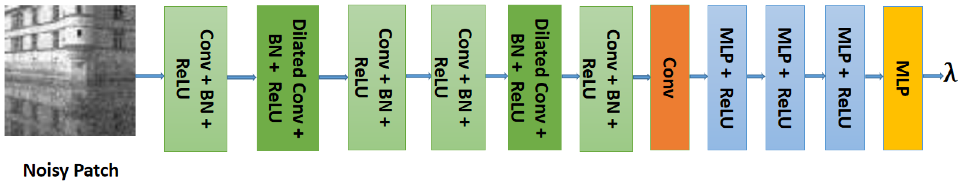
3.3.2. $\lambda$ Estimation

The sparse coding $\alpha$ is obtained by addressing a regularization parameter ${\lambda }_k$ for each noise patch $y_k$, to regulate the sparsity. The regularization parameter is fitted based on the noise level and signal characteristics. The optimal sparsity coefficient $\widehat{\alpha }$ is evaluated and utilized with the sparse reconstruction theory formula $\widehat{x}=D\widehat{\alpha }$ to reconstruct the denoised image patch $\widehat{x}$ with high precision. This accomplishes the mapping of the noisy image to the denoised image. In this study, a data-driven approach to realize this mapping is proposed, through learning a regression function.

$$x_k=f_{\tau }\left(y_k\right)$$

(11)

This paper proposes a network that performs various tasks, such as estimating ${\lambda }_k$, solving sparse coding, updating parameters, and mapping noisy and denoised images. The network, as illustrated in Figure 3, estimates $\lambda$ by utilizing seven layers of hybrid dilated convolution paired with batch normalization (BN). The network also uses four layers of multilayer perceptron, where every hidden layer is connected to a Relu activation function. The pooling operation in some cases can extract valuable features, but it can also result in the loss of significant image details, which is not desirable for the denoising task at hand. Therefore, a pooling operation is not employed, since the model’s input and output size remain unchanged.

Figure 3. $\lambda$ estimation network.

To conclude, the proposed network f is a parameterized function of $\tau$ (the parameters of the network computing $\lambda$), t (the step-size in the ISTA algorithm), D (the dictionary), and w (the weights for the patch-averaging).

3.3.3. Patch Reconstruction

This stage reconstructs the cleaned version $\widehat{x}$ of the patch y using D and the sparse code $\widehat{\alpha }$, which is given by $\widehat{x}=D\widehat{\alpha }$. D and $\widehat{\alpha }$ are both updated in the aforementioned network.

3.4. Patch Averaging

Now we can discuss the complete system architecture. First, we will decompose the input image into fully overlapping patches, and then process each damaged patch through the aforementioned patch denoising stage. Finally, we will average these damaged patches, to reconstruct the image. In the final stage, we realize the learned weighted combination of patches. The weight of each patch is represented as $w\in R^{n\times n}$, so the retrieval of the reconstructed image is obtained as

$$\widehat{X}=\frac{{\sum }_i{A}_i^T\left(w\odot {\widehat{x}}_i\right)}{{\sum }_i{A}_i^{T}w}$$

(12)

Obtaining a denoised image X is feasible, with ⊙ representing the Schur product and $A_i$ signifying the ith operator extracted from the image.

3.5. Loss Function

Considering a noisy image Y, we use a denoising network to produce a denoised image X given that $X=F\left(Y\right)$, where F represents the end-to-end denoising network. We derive the loss function from this specific mapping:

$$L=\sum _i{∥X_i-F\left(Y_i\right)∥}_2^2$$

(13)

The network is trained using data to minimize the loss function. Here,${\left\{X_i\right\}}_i$ and ${\left\{Y_i\right\}}_i$ denote the training images and their noisy counterparts, respectively. The noise added is zero-mean and white Gaussian iid.

4. Simulation Results

Here, we present the simulation experiments of our proposed model, aiming to demonstrate the superiority of the fusion of traditional sparse representation theory and deep learning over conventional state-of-the-art denoising algorithms such as BM3D and WNNM. Moreover, our model was expected to outperform DnCNN in terms of objective metrics and image detail preservation.

4.1. Simulation Experiments

Training settings: We trained our model using the BSD400 dataset as the training dataset, comprising 400 grayscale images of natural and face scenes with dimensions $481\times 321$ and $321\times 481$ pixels. The images during training were randomly cropped to $200\times 200$ patches with a stride of 40. The input noise during training was independent and identically distributed Gaussian noise, with a mean of zero, and the noise level $\delta$ was specified. We trained several models for each noise level: $\delta$ = 15, 25, and 50. Our model used the mean squared error (MSE) as the loss function, and the optimization algorithm used to minimize this loss was Adam. Our model’s initial learning rate was set to $1\times {10}^{-3}$ and decayed to $1\times {10}^{-5}$ over 9 epochs. The learning rate was set to $1\times {10}^{-3}$ for the first three epochs, $1\times {10}^{-4}$ for the next three epochs (i.e., the fourth to sixth epochs), and $1\times {10}^{-5}$ for the last three epochs (i.e., seventh to ninth epochs). The DCT matrix was overcomplete and initialized using the K-singular value decomposition (KSVD) [7] method. The parameter t was set using the squared spectral norm of the DCT matrix. The Kaiming uniform method was used to initialize the other network parameters, including Conv, BN, and MLP.

Validation settings: The trained models were evaluated using two datasets, BSD68 and Set12. The objective evaluation metric used in this study was the peak signal-to-noise ratio, which was calculated based on the following formula:

$$\mathit{PSNR}=10·{\log }_{10}\left(\frac{{\mathit{MAX}}_I^2}{\mathit{MSE}}\right)$$

(14)

where $MA{X}_I$ represents the maximum possible pixel value (usually 255 for 8-bit grayscale images), and $MSE$ is the mean squared error.

In this paper, we utilized PyTorch 1.2.0 and Python 3.7 to train and test our proposed model. We conducted all experiments in the Windows 10 operating system with a 3.60 GHz clocked AMD Ryzen 7 3700X CPU, 32 GB of RAM, and an Nvidia GeForce RTX 2080 Ti GPU. To speed up the GPU training process, we used Nvidia CUDA 10.0 and cuDNN 7.4. It took approximately 20 h to train the grayscale Gaussian denoising model.

4.2. Analysis of Simulation Results

Evaluating the effectiveness of an algorithm involves considering both objective and subjective criteria. The objective criterion usually measures the average peak signal-to-noise ratio (PSNR) of the algorithm across all images in a given dataset, where higher values suggest a better performance. In contrast, an improved subjective evaluation results from preserving more image detail and minimizing edge artifacts.

Table 1 shows that average PSNR (dB) of different methods on BSD68 with different noise levels of 15, 25, and 50. The red and blue colors mark the highest and second-best denoising performance in Table 1, respectively. Our proposed method outperformed BM3D [8], KSVD [7], WNNM [18], TNRD [21], DnCNN [35], and MLP [33] at various noise levels. Our method demonstrated a 0.02 dB improvement over DnCNN, a 0.28 dB improvement over TNRD, a 0.67 dB improvement over BM3D, and a 0.37 dB improvement over WNNM at a noise level of 15. Similar results were observed for noise levels of 25 and 50, demonstrating that the combination of sparse representation theory and deep learning is a powerful approach, which leverages the accurate prior knowledge provided by sparse representation to complement deep learning techniques. These results confirm the effectiveness of our proposed method and validate the feasibility of our approach.

Table 1. Average PSNR (dB) of the different methods on BSD68 with different noise levels of 15, 25, and 50.

Method	$\delta$ = 15	$\delta$ = 25	$\delta$ = 50
BM3D	31.07	28.57	25.62
KSVD	30.91	28.32	25.03
WNNM	31.37	28.83	25.87
MLP	-	28.96	26.03
TNRD	31.42	28.92	25.97
DnCNN	31.72	29.19	26.23
Ours	31.74	29.22	26.24

Table 2 shows the average SSIM (dB) of the different methods on BSD68 with different noise levels of 15, 25, and 50. SSIM (structural similarity index) is a widely used image quality assessment metric that measures the structural similarity between two images. It takes into account the luminance, contrast, and structural information of images and produces a score between 0 and 1, where 1 indicates that the two images are identical. It can be observed that the SSIM and PSNR rankings of the denoising algorithms were consistent. Therefore, in our evaluation experiments, we used PSNR as the objective evaluation metric and image detail preservation as the subjective evaluation metric.

Table 2. Average SSIM (dB) of the different methods on BSD68 with different noise levels of 15, 25, and 50.

Method	$\delta$ = 15	$\delta$ = 25	$\delta$ = 50
BM3D	0.8717	0.8013	0.6864
KSVD	0.8692	0.7876	0.6322
WNNM	0.8766	0.8074	0.6984
TNRD	0.8813	0.8157	0.7029
DnCNN	0.8826	0.8186	0.7072
Ours	0.8837	0.8199	0.7088

Table 3 depicts the average peak signal-to-noise ratio (PSNR) (dB) of the various image denoising methods on Set12 with varying noise levels of 15, 25, and 50. The highest and second-best performances in Table 2 are marked with red and blue lines, correspondingly. Our proposed method exhibited a superior performance to the other methods tested, as revealed in Table 2. Notably, our method surpassed the DnCNN and WNNM techniques, with a PSNR improvement of 0.03 dB and 0.19 dB, respectively, for a noise level of 15. Remarkably, we observed that the performance of WNNM on Set12 was nearly comparable to that of DnCNN and our proposed method, whereas it significantly outperformed KSVD. We conjecture that this could be attributed to the fact that both WNNM and BM3D exploit nonlocal self-similarity, which can facilitate the acquisition of accurate structural information and lead to better noise reduction by discovering similar pixel blocks across the entire image. This characteristic is also leveraged in our algorithm.

Table 3. Average PSNR (dB) of the different methods on Set12 with different noise levels of 15, 25, and 50.

Method	$\delta$ = 15	$\delta$ = 25	$\delta$ = 50
BM3D	32.37	29.97	26.72
KSVD	31.75	29.17	25.58
WNNM	32.70	30.26	27.04
MLP	-	30.03	26.78
DnCNN	32.86	30.43	27.18
Ours	32.89	30.45	27.16

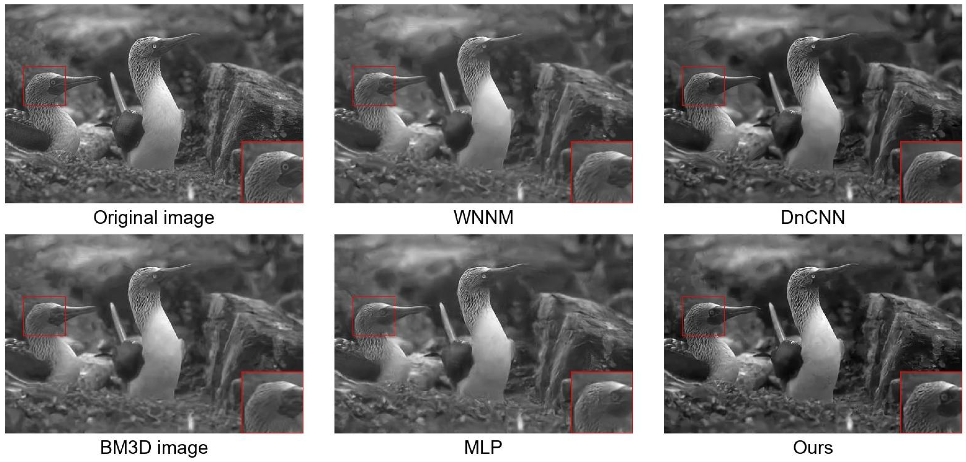
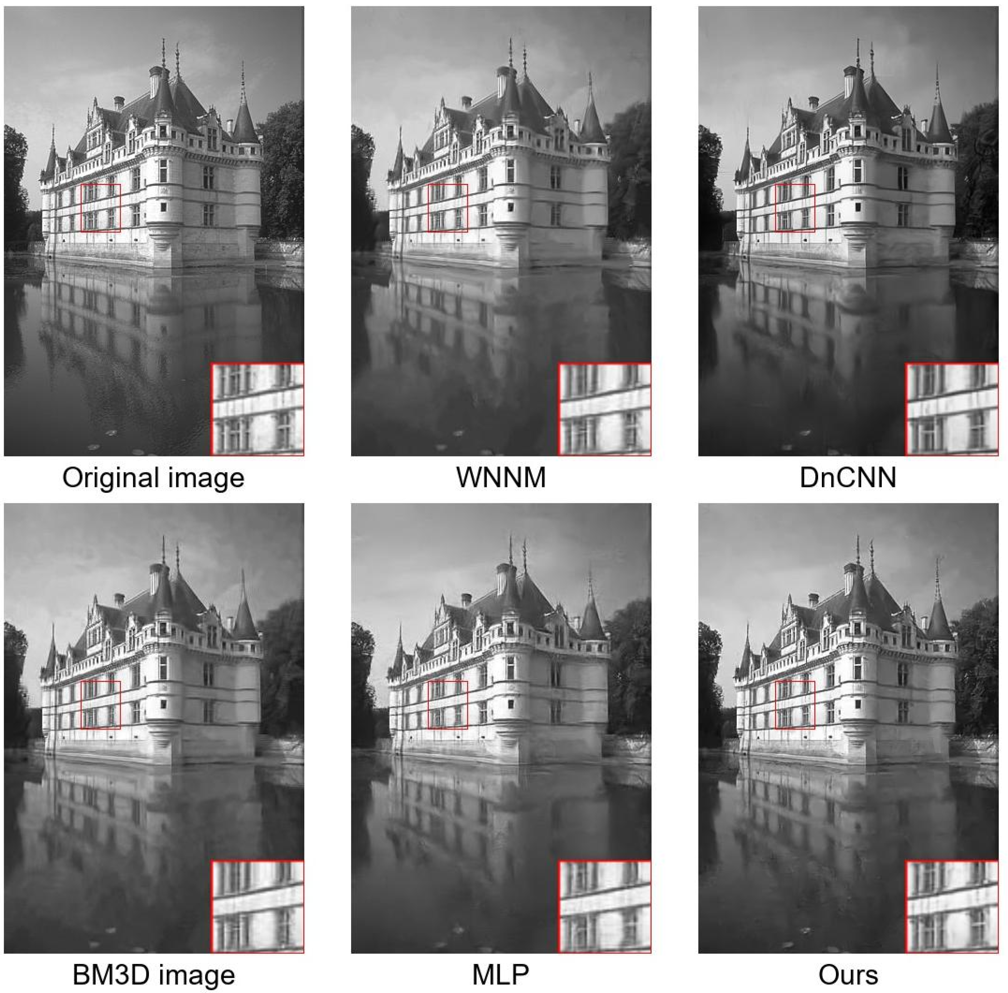
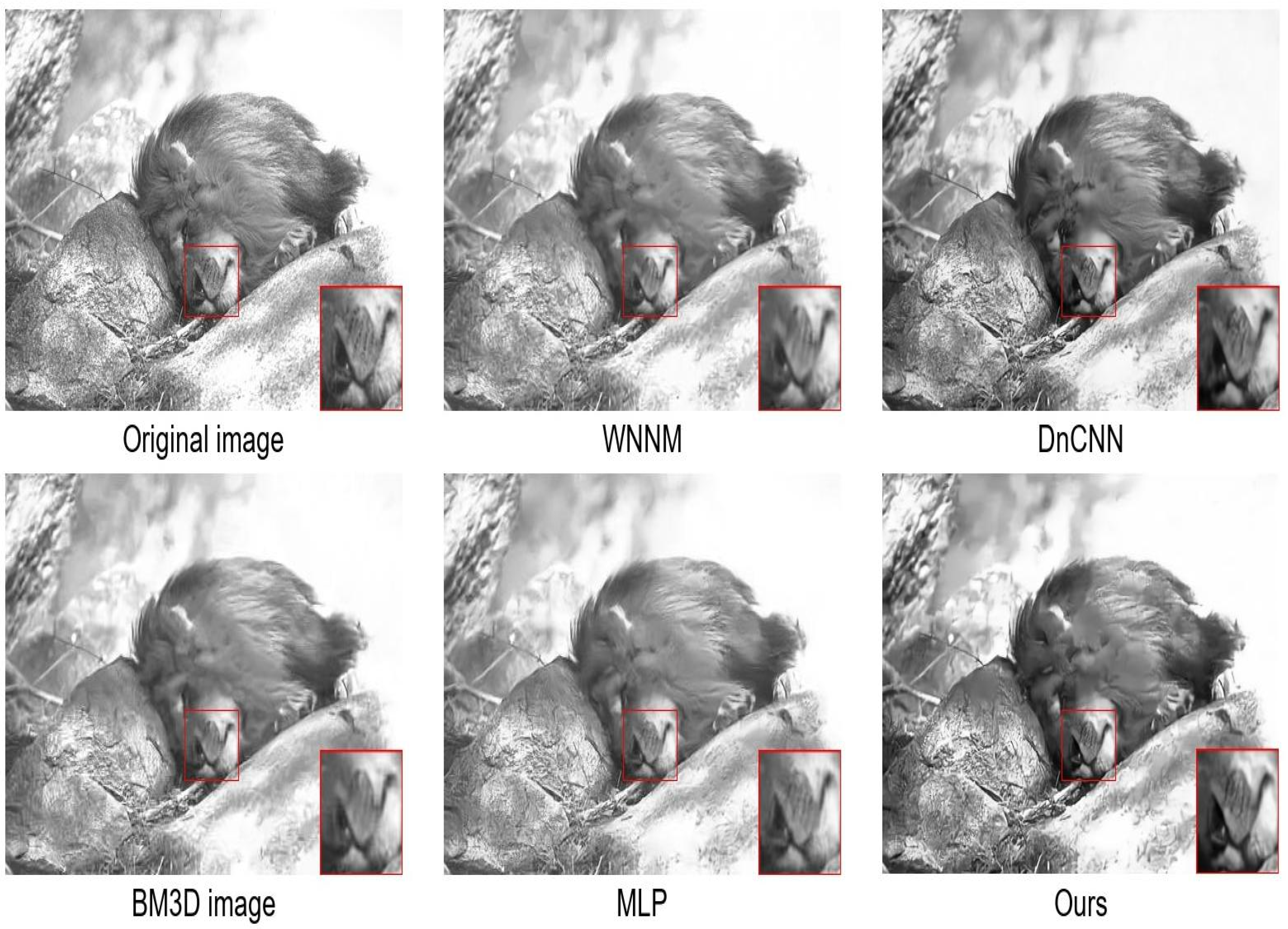
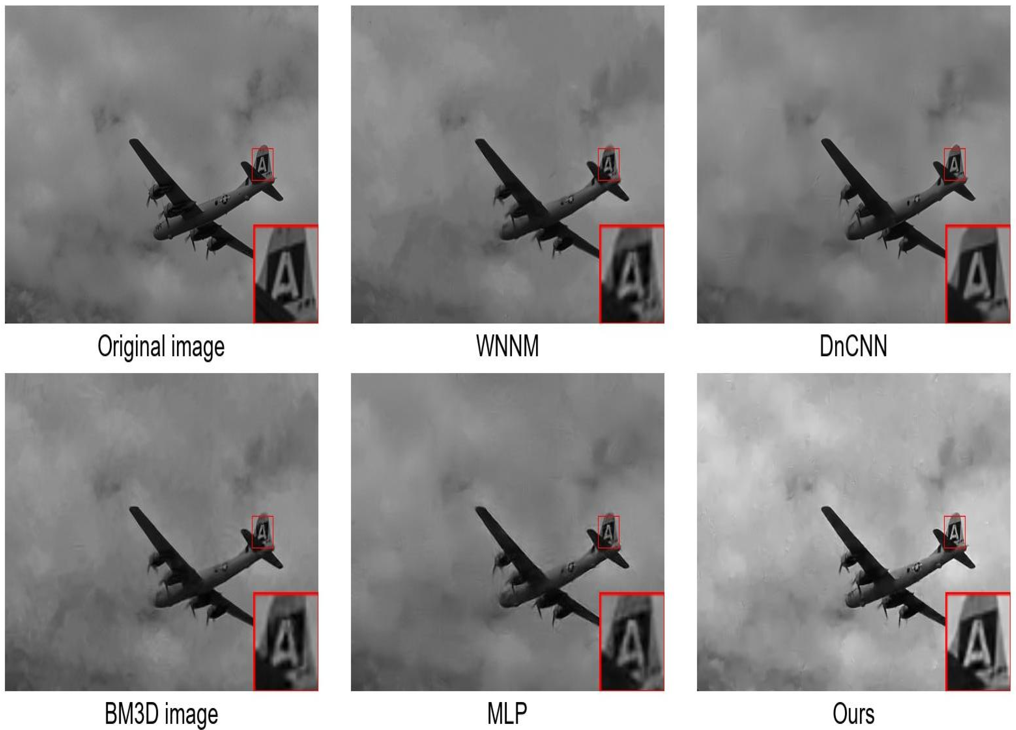
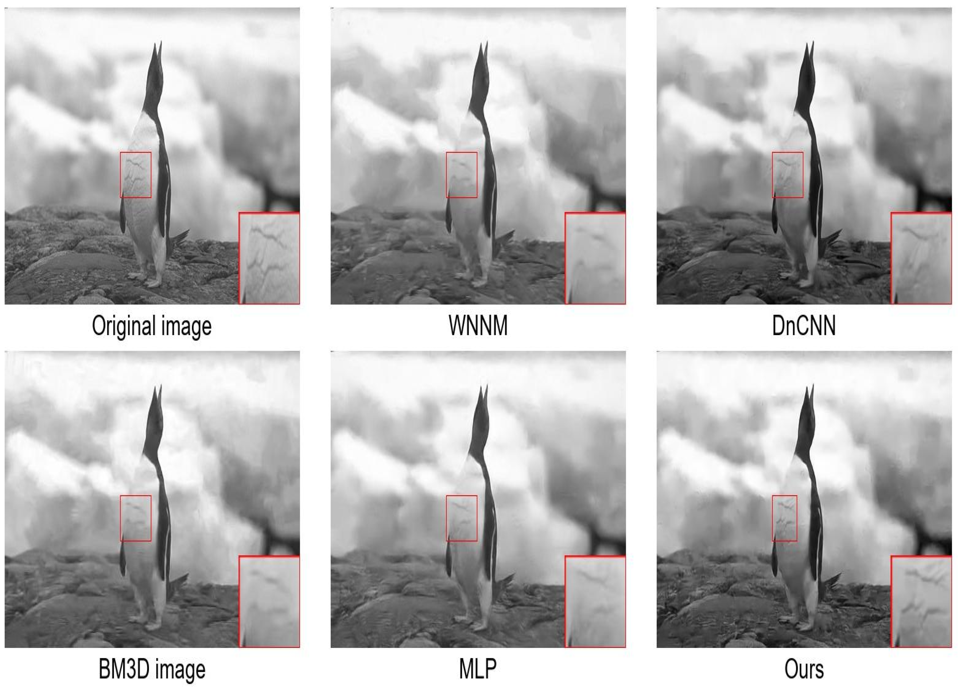
Figure 4, Figure 5, Figure 6, Figure 7 and Figure 8 present the visual performance and corresponding peak signal-to-noise ratio (PSNR) values in decibels (dB) of the different methods on the five images in the BSD68 dataset at a noise level of 25. The red box in the Figure 4, Figure 5, Figure 6, Figure 7 and Figure 8 indicates the enlargement of a detail. Overall, our proposed method and the DnCNN method achieved the leading denoising quality among the five methods compared, in terms of both noise reduction and detail preservation. Specifically, as shown in Figure 4, the detail enlargement of the bird’s eye reveals that only our method and the MLP method fully preserved the details of the eyeball, and our method achieved the clearest result. Additionally, Figure 6 shows that the detail enlargement of the animal nose indicates that our method preserved the texture details of the nose most clearly and closest to the original image. Furthermore, Figure 8 indicates that the detail enlargement of the penguin’s abdomen reveals that our method preserved the texture details of the abdomen the best, followed by the DnCNN method. Combining the results in Table 1 and Table 2, and the performance shown in Figure 4, Figure 5, Figure 6, Figure 7 and Figure 8, we believe that our proposed method achieved the predetermined goal. Our method performed significantly better than traditional methods such as the BM3D and WNNM methods on the public datasets, while being able to compete with DnCNN methods in terms of objective metrics and image quality.

Figure 4. Denoising results of the different methods on an image from BSD68 with $\delta$ = 25. Original image, WNNM/30.42 dB, DnCNN/30.75 dB, BM3D/30.33 dB, MLP/30.47 dB, Ours/30.78 dB.

Figure 5. Denoising results of the different methods on an image from BSD68 with $\delta$ = 25. Original image, WNNM/29.76 dB, DnCNN/30.19 dB, BM3D/29.53 dB, MLP/29.72 dB, Ours/30.17 dB.

Figure 6. Denoising results of the different methods on an image from BSD68 with $\delta$ = 25.Original image, WNNM/27.30 dB, DnCNN/27.68 dB, BM3D/27.11 dB, MLP/27.51 dB, Ours/27.72 dB.

Figure 7. Denoising results of the different methods on an image from BSD68 with $\delta$ = 25. Original image, WNNM/37.20 dB, DnCNN/38.41 dB, BM3D/36.94 dB, MLP/37.53 dB, Ours/38.36 dB.

Figure 8. Denoising results of the different methods on an image from BSD68 with $\delta$ = 25. Original image, WNNM/32.56 dB, DnCNN/33.05 dB, BM3D/32.41 dB, MLP/29.72 dB, Ours/33.09 dB.

5. Conclusions

In this paper, we propose a deep convolutional denoiser based on sparse representation that combines the strengths of sparse representation and deep learning. Sparse representation provides accurate prior knowledge, while deep learning networks can use large amounts of data to automatically train parameters, overcoming the limitations of traditional denoising methods. The ideal combination of sparse coding and deep learning networks is reflected in the simulation results, where our proposed method outperformed both the traditional denoising algorithms, such as BM3D and WNNM, and DnCNN in terms of objective metrics and detail preservation. This demonstrates that our proposed approach is effective and highly competitive.