Article

Drone Deployment Algorithms for Effective Communication Establishment in Disaster Affected Areas

by
Bivin Varkey Varghese
,
Paravurumbel Sreedharan Kannan
,
Ravilal Soni Jayanth
,
Johns Thomas
and
Kavum Muriyil Balachandran Shibu Kumar
*,†
Department of Computer Science and Engineering, Rajiv Gandhi Institute of Technology, Kottayam 686501, India
*
Author to whom correspondence should be addressed.
These authors contributed equally to this work.
Computers 2022, 11(9), 139; https://doi.org/10.3390/computers11090139
Submission received: 9 August 2022 / Revised: 4 September 2022 / Accepted: 10 September 2022 / Published: 15 September 2022

Abstract

:
Communication establishment is crucial for rescue operations in disaster affected areas. A standard tool for communication is the use of cell phones. However, they can be useless in situations where the cellular network’s base stations are damaged in a disaster. A contemporary approach to re-establishing a communication network is by hosting base stations in drones. However, low battery life and difficulty in calculating the number of drones needed in different terrains are limitations of the above approach. This paper introduces a novel terrain-aware algorithm that calculates the minimum number of drones needed to cover an area with no voids in the network coverage. Our method ensures that the drones are deployed at optimal heights to maximize the average leftover energy in the network. We apply the algorithm for an actual location in Pettimudi, India and find the optimal number and positions of the drones to cover the area effectively without voids. In addition, we provide a simulation of the the communication establishment using above drones, and our experiments yield an average network efficiency of 98%, showing the effectiveness of our method.

1. Introduction

The human race has always shown immense potential to manage and cope with natural disasters. As humans, we have developed various techniques to prevent and mitigate these life-threatening disasters. Setting up a communication infrastructure is widely discussed among such techniques, as normal means of communication might be devastated during disasters [1]. One of the most critical parts of disaster response is effective information exchange between information sources, emergency managers, and those impacted by the disaster event. During disaster events, the terrestrial communications infrastructure, such as mobile phone networks, TV networks, and radio networks, are frequently affected by the disaster impacts. This situation has a considerable impact on all preparedness, response, and recovery processes in disaster conditions [2]. Hence, there is always a need to maintain the entire disaster affected region under communication coverage throughout the rescue operations.
The communication between disaster management organizations, the general public, and other actors is a critical and fundamental factor in providing a quick and opportune response to all aspects of the disaster event. Many practical experiences show the importance of communication during a disaster [3].
One such case is the Pettimudi Landslide [4] that occurred in India on 6 August 2020. The disaster resulted in the snapping of communication lines and blockage of roads due to the uprooting of trees. This made it challenging for the local search groups to contact the base station. It was reported in the leading dailies that rescue groups had to stay near dead bodies for nearly three hours [5]. They needed to wait for other teams to arrive with a vehicle or wireless device before they were able to share messages. The rescue operations were effective only after the restoration of mobile towers.
Another case is the Sichuan Earthquake [6] that occurred in China on 12 May 2008. During the disaster, telecommunication systems were affected. The Chinese government activated the use of the national communications satellite network to recover communication services in all affected areas and support other solution implementations for different types of data exchange between the entities in charge of disaster management. The importance of communication during a disaster can be seen in other events as well. Recent examples include Typhoon Faxai in 2019 in Chiba, Japan [7] and bush fires of New South Wales in 2019–2020 [8]. In the former case, the damage mainly happened to the roofs of buildings, and prompt damage assessment was able to quickly facilitate disaster insurance relief. The latter case required aerial monitoring of areas in order to understand the status and severity of the bush fires.
Drones are increasingly becoming a viable alternative to conventional cellular infrastructure in disaster-struck regions thanks to their low cost and availability [9]. Their easy availability and low weight make them potential candidates as communication support in any terrain [10]. An example of such a communication network establishment is shown in Figure 1. Drones can easily be deployed to the affected region from one or more base stations, although performance in terms of flight time due to battery power restrictions, the number of drones required, and terrain constraints all remain matters of concern [11].
This paper considers the idea of deploying drones to restore the communication system in a post-disaster area. As proposed here, a swarm of drones carrying network receptors is deployed in the disaster struck location. The drones can be deployed quickly and conveniently for temporary coverage until more permanent solutions are deployed, allowing recovery operations to continue smoothly. Using this method, the mobile phone network is restored and people can use their mobile phones to notify the concerned authorities. This enables fast establishment of reliable communications in any environment.
A significant concern with the above approach is the large number of drones required to cover the affected region. In addition, it is necessary to ensure that the deployed drones have sufficient leftover energy to serve the region long enough to conduct the rescue operation. Hence, we formulate a novel region-filling algorithm that brings the entire disaster affected area under drone network coverage without creating voids. Our algorithm considers the terrain data (altitude of various points in the region). We deploy the drones at optimal heights in order to maximize the system’s average leftover energy. To the best of our knowledge, this approach towards communication establishment in a disaster affected area using stationary drones with maximum average leftover energy while minimizing the number of drones required is the first of its kind to be reported. The main research contributions of the paper can be summarized as follows:
  • Development of a terrain-aware region-filling algorithm that covers the entire disaster affected area under a cellular network.
  • Minimization of the required number of drones while maximizing the average leftover energy of the system.
  • A proof that our method uses the minimum number of drones possible.
  • Application and evaluation of the above methods using the parameters of a real location in Pettimudi, India.
  • A simulation of the region-filling algorithm for the terrain of Pettimudi.
The rest of this paper is organized as follows. Section 2 describes the state-of-the-art of the literature on the topic. Section 3 details the various algorithms we formulated. Section 4 explains the experiments and simulations we conducted and their results. Finally, the paper ends with a conclusion section describing our future work.

2. Related Works

There have been trials in establishing communication in a post-disaster region. AT&T is an American telecommunication company that provides AT&T Network Disaster Recovery (NDR) [12] units that restore their network in a disaster area by bringing in portable cellphone towers on trucks called Cell on Wheels (COW) [13]. The NDR team was a great aid during the California wildfires (2017), Hurricane Irene (2011), Hurricane Irma (2017), and Hurricane Maria (2017) [14], although transporting the COW is difficult when roads are damaged due to disaster impact. Furthermore, COW is unsuitable for disasters such as floods, landslides etc.
Another method is the use of satellite phones or two-way radios as communication devices [15]; however, these devices are not affordable for the general public, and government regulations may prevent the general public from using these devices. In addition, it is not easy to track their locations.
Using drones for communication is a growing research field due to their on-demand deployment and high flexibility [16]. Park et al. [17] proposed a formation control algorithm for a drone-based network in a planar region. The algorithm increases the network throughput by improving the network infrastructure. Zhang et al. [18] proposed deployment algorithms for a drone network that maximize the leftover energy of all drones. The algorithm takes account of any no-fly-zone constraints in the operational region. Ruan et al. [19] proposed a multi-drone coverage deployment model that focuses on efficient network coverage and energy conservation. Pankaj Kumar et al. [20] provided a framework for a network that uses drones as a relay node to achieve good quality of service, better spectral efficiency, and improved diversity. Mozaffari et al. [21] proposed a novel framework for a drone-enabled antenna array system that provides better service to users. It considers each drone as an element in the antenna array system and optimizes the drone positions in the array to maximize the antenna gain and minimize the service time for the ground users. Namvar et al. [22] developed an algorithm for deploying a heterogeneous set of drones that provide maximum wireless coverage for ground users in a planar area.
There have been attempts to improve the performance and efficiency of drone-based networks. Thibbotuwawa et al. [23] derived the energy consumption of drones and determined the influence of various parameters that affect the energy of the drones. Theys and Schutter [24] provided experimental results on the relationship between various factors of a quadcopter. Sundaresan et al. [25] developed the designs of low-altitude drone networks that provide Long-Term Evolution (LTE) connectivity. Panda et al. [26] proposed a drone-based network that uses Wi-Fi as an emergency communication network for disaster management. Li et al. [27] proposed a deployment algorithm for drone-based networks that improves network throughput and coverage in the disaster area. Ishigami and Sugiyama [28] proposed a method to improve drone network throughput by controlling the drones’ height with respect to the number of users. Shakhatreh et al. [29] proposed an algorithm for drone deployment that minimizes the number of drones required for the network.
Lyu et al. [30] introduced a spiral algorithm that aims to minimize the number of base stations mounted on grounded vehicles. However, in situations where such vehicle access is limited, the technology is not applicable at all. A research paper by Plachy et al. [31] discussed the positioning of base stations in unmanned aerial vehicles. They developed an algorithm to find the optimal positions of the base stations through association of the Genetic Algorithm (GA) and Particle Swarm Optimization (PSO) evolutionary strategies. However, GA is computationally complex and PSO tends to fall into local optima. A paper by Ruzicka et al. [32] introduced a conditional generative adversarial neural network-based algorithm to optimize network coverage in similar situations. Their simulations showed that the algorithm converges to a quasi-optimal solution.
Recently, drone network-based disaster recovery has attained even wider acceptance. Furutani and Minami [33] discussed the various aspects of using drones for disaster risk mitigation and crisis response, especially in Japanese contexts. They explain the need for drones in disaster risk reduction, the different technologies applicable to this use case, and a variety of such cases in Japan. There have been studies focusing on the communication aspects as well; Chen and Cheng [34] proposed Reconfigurable Intelligent Surface (RIS) technology to support communications in post-disaster areas. In [35], the authors explained how a drone equipped with RIS can be used to cover users with an mmWave base station. An energy-aware multi-armed bandit algorithm is used to cover several high-capacity network hotspots while minimizing the energy consumption. In [36], the authors proposed the use of access and gateway drones to support communication over disaster-affected areas. An access drone collects information from its assigned area and flies to the nearby gateway drone to transfer the information. In order to avoid two access drones targeting the same gateway, the authors employ two multi-armed bandit-based algorithms, namely, the Kullback–Leibler upper confidence bound (KLUCB) and minimax optimal stochastic strategy (MOSS) algorithms. However, frequent flying can drain the energy of drones very quickly in this case.
The above works show that a drone-based network is a good option for establishing communication in a post-disaster area. However, there are gaps in the current research with respect to ensuring complete coverage while the minimum number of drones. In the above-mentioned drone deployment algorithms, the terrain is assumed to be a planar region, which can create bottlenecks in real-world implementation scenarios. Furthermore, maximization of average leftover energy in the system is another area that needs to be addressed in order to enable system operations over sufficiently long durations. Hence, in this study we concentrate on the development of a terrain-aware, deterministic, and energy efficient region-filling algorithm that uses the minimum number of drones to cover the entire disaster-affected area with no network voids.

3. Proposed Methods

3.1. Problem Statement

We aim to formulate a drone deployment algorithm to establish a mobile network for disaster management. The main considerations can be summarized as follows:
  • To develop a strategy for deploying drones to maintain the maximum possible average leftover energy and thereby increase the overall hovering time of all drones deployed.
  • To develop a region-filling method that guarantees coverage over the whole region with the minimum possible number of drones.
  • To deploy drones for communication establishment based on terrain and altitude analysis.
  • To determine the number and positions of base stations required to facilitate the network.

3.2. Methodology

Our aim is to formulate a swarm of drones in a disaster affected area to facilitate establishment of communication network without forming voids. A first-hand strategy to this end is the use of an AI-based method such as Particle Swarm Optimization (PSO) [37,38]. However, PSO-based algorithms are prone to falling into local optima, and the rate of convergence in the iterative process may be low [39]. Other AI-based algorithms, such as Genetic Algorithms and Simulated Annealing, face the same issues, apart from being too slow. As concerns to neural networks and deep learning, they are computationally expensive and often require frequent training to produce accurate results [40].
In our case, we have to produce deterministic positions for the drones in order to fully ensure network coverage in the disaster affected location while at the same time ensuring maximum average leftover energy to service the network. This needs to happen in a time-bound way using available computational resources. Therefore, we aim to develop a terrain-aware region-filling algorithm which is less computationally intensive. Here, we find the number and positions of drones and base stations required to create a robust temporary network in the target region. We accomplish this by considering the terrain, intending to cover the entire region without voids while minimizing the number of drones and maximizing their average leftover energy.
The drone deployment algorithm we propose consists of a preprocessing module and a region-filling module. Preprocessing involves obtaining terrain data on the disaster-struck region and then converting this into a suitable data structure for the region-filling algorithm. The region-filling algorithm provides a powerful solution to the above problem. The output of the region-filling algorithm contains a list of three-dimensional coordinates of the positions of drones, with base station indication, leftover energy, and hovering time. Finally, we simulate the deployment of drones based on the positional information obtained from the Region-Filling algorithm. An outline of the process is shown in Figure 2.

3.3. Preprocessing

The first step in preprocessing is to obtain the terrain data of the disaster struck region. This information is obtained in JSON format and then converted to the Cartesian Coordinate system required by the region-filling algorithm. The elevation profile of a region is commonly available in Degree Minute Second (DMS): Altitude format [41].
In our work, the Universal Transverse Mercator (UTM) coordinate system is used instead of the latitude–longitude coordinate system in order to precisely determine the distance between two points. If the two points are inside a UTM zone, the distance between the two points can be easily determined using the UTM coordinates [42].

3.3.1. The Preprocessor Module

The actions of the preprocessor module include:
  • Construction of the Height Matrix(H) data structure.
  • Calculation of the environment parameters required by the region-filling algorithm.

Height Matrix Data Structure

The Height Matrix (H) data structure stores the normalized altitudes of different locations in the disaster affected area. The altitude data are obtained as a JSON file (Coordinate: Altitude format). A normalization factor is calculated by finding the altitude of the lowest-lying point in the terrain. The normalized altitudes are obtained by subtracting the normalization factor from each altitude, then populated to the Height Matrix data structure.

Environmental Parameters
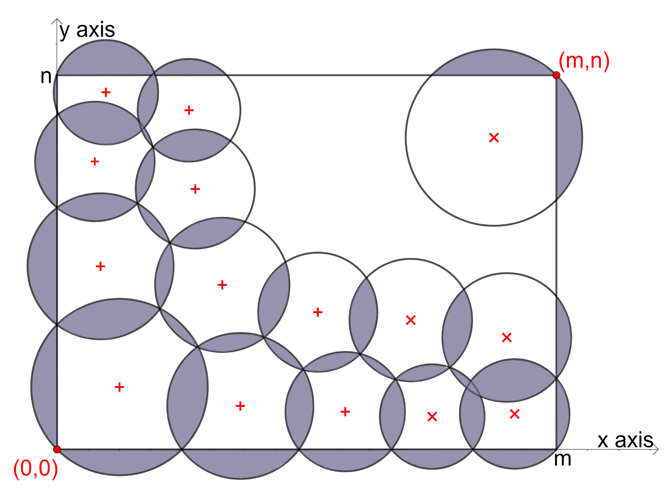
We define the various environmental parameters specific to the drones and the terrain in Table 1. We note the average altitude of the terrain from H, then add a threshold value based on the terrain elevation profile. The sum of the average normalized altitudes and threshold value forms H m i n .

3.4. Region Filling

Region filling is the core part of drone deployment; here, we implement a strategy to cover a rectangular region without any voids using circles of different radii. Each circle represents the coverage area of each drone. A drone deployed at a particular height is considered to have a cone-shaped coverage region, as shown in Figure 3. Usually, when a rectangular region is filled using circles, there will be voids in between. However, we use overlapping circles to avoid leaving any regions without network coverage. As this leads to wastage or redundancy of coverage, we aim to minimizing this wastage, and thereby the required number of drones.
We define H m a x as the maximum altitude (in km) where a drone can be positioned such that any mobile device connected to it has sufficient network strength. Furthermore, H m a x must be greater than the tallest obstacle within the whole region. While the region-filling algorithm performs filling coverage in two dimensions, it incorporates terrain data at various points for the practical deployment of drones.

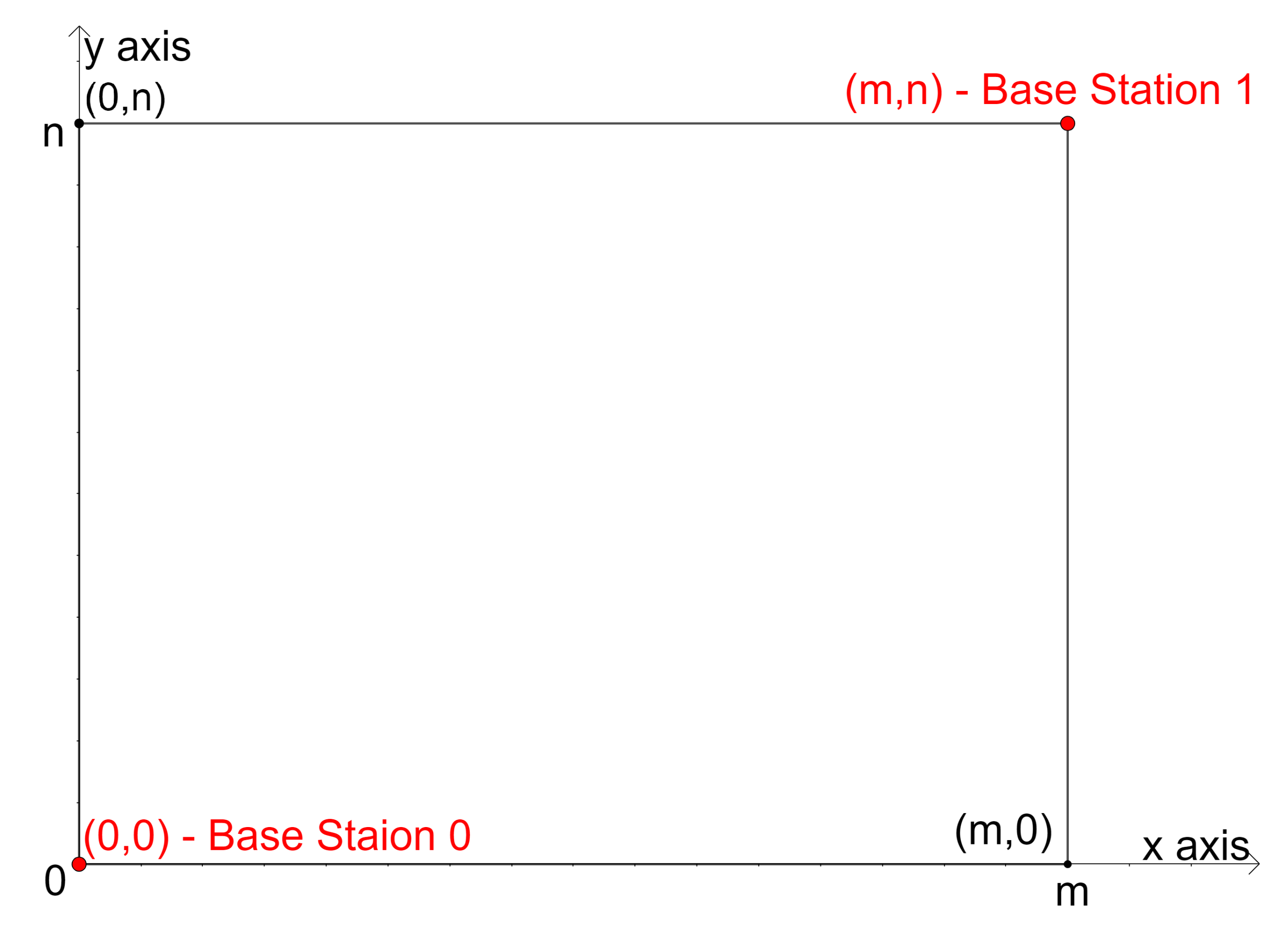
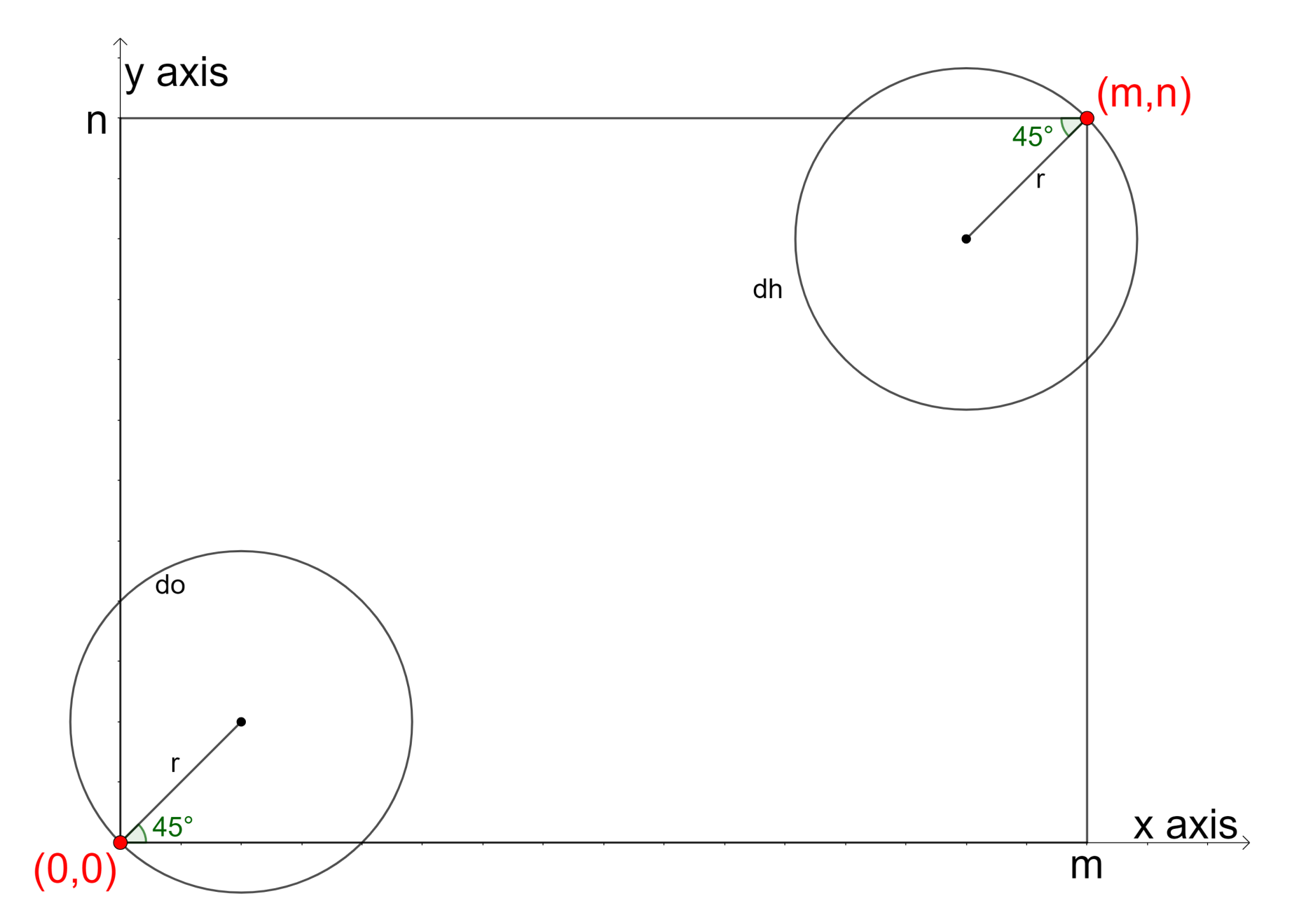
3.4.1. Determining the Number and Positions of Base Stations

Drones are deployed from corresponding base stations. It is necessary to determine both the number of base stations required and their positions. In order to fix the base stations in a deterministic way, we adopt a strategy whereby they are always placed at the corners of the rectangular region. Therefore, one, two, three, or four base stations are possible for a rectangular region. Increasing the number of base stations reduces the required number of drones, as the drones close to base stations can be deployed at greater heights, thereby increasing the coverage area. However, our experiments (detailed in Section 4) show that increasing the number of base stations beyond two does not provide any clear advantage; hence, we fix the number of base stations at two, located at opposite corners. One base station is fixed as the origin (0, 0) and the other as (m, n), as shown in Figure 4.

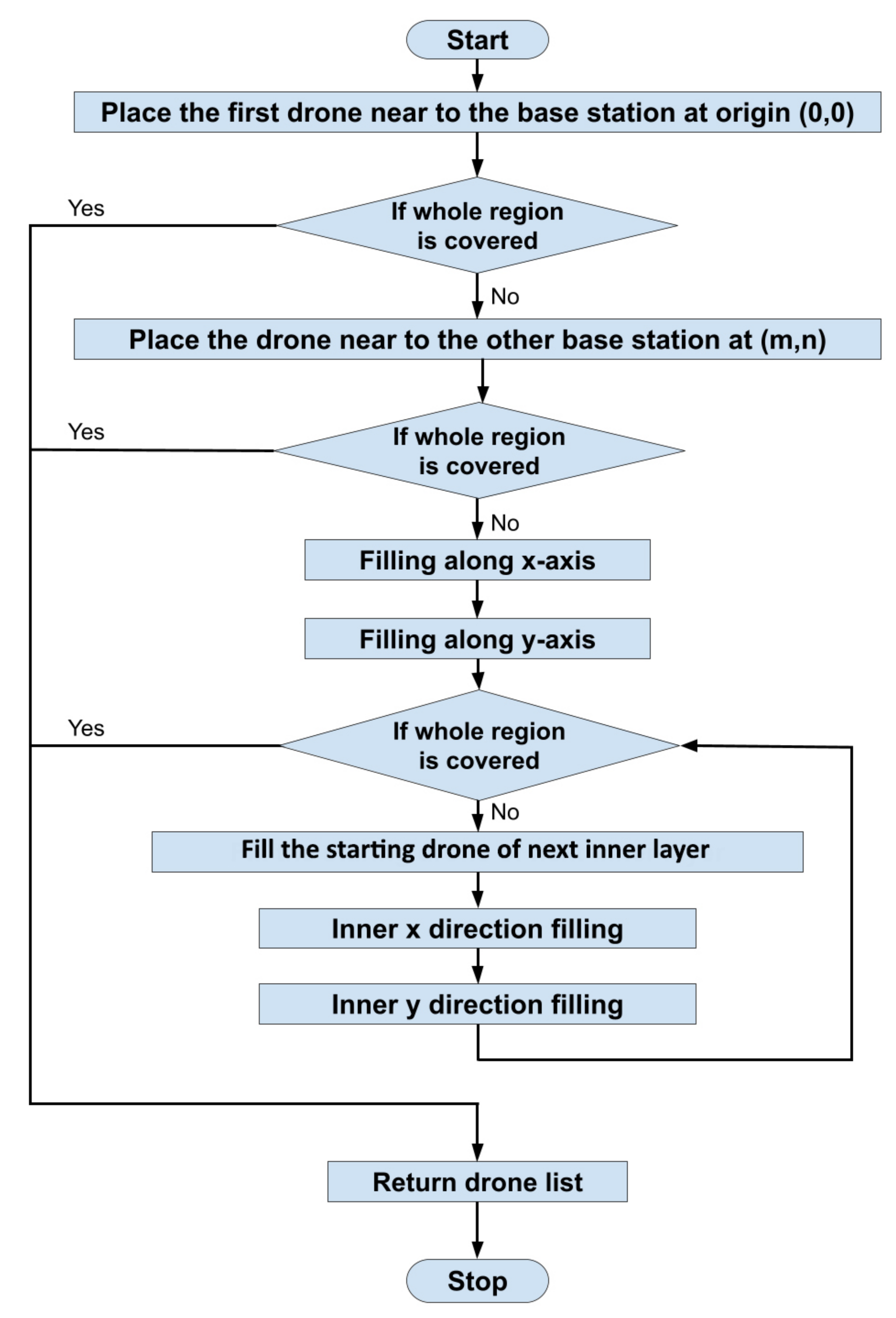
3.4.2. Outline of the Region-Filling Algorithm

The algorithm begins to fill the area with drone coverage, specifically, circles, from the origin towards the other corner. This is achieved by filling each x-directional and y-directional inner layer at each iteration until the whole region is covered. The algorithm considers the following attributes of a drone object d:
  • ( x , y ) x and y coordinates of the position of a drone
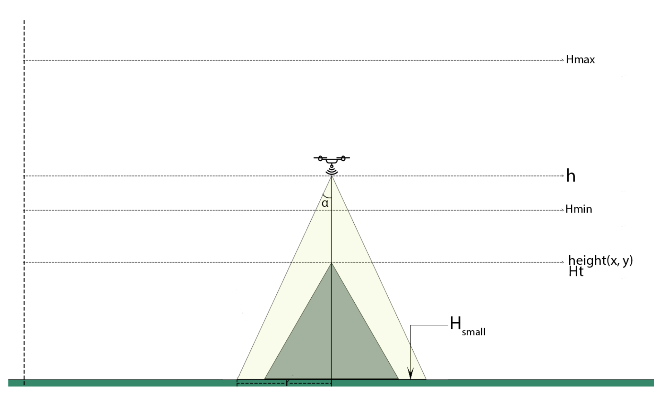
  • r—radius of the cone-shaped network coverage
  • h—height of the cone-shaped network coverage
  • b—an indication of the base station; a value of 0 means the base station of the drone is at (0, 0) and 1 means the base station of the drone is at (m, n)
  • e—leftover energy of the drone when the drone reaches its assigned location starting from its base station
  • h r e f —the maximum value among the heights of reference points associated with each drone, which is needed in order to cope with the terrain of the affected region
  • n o r t h , s o u t h , w e s t , e a s t —the northern, southern, western, and eastern neighbouring drones of the network drone
We use h r e f to denote the height of the reference point of a drone. There are many reference points associated with each drone object. These points can be the corner points where a circle intersects other circles, the x-axis, or the y-axis; thus, h r e f is the maximum value of the heights of all reference points of a particular drone. A view of reference points and h r e f is shown in Figure 5.
The algorithm fills the rectangular region layer by layer, starting from the base station at (0,0) and moving towards the one at (m, n) while assigning each drone to the nearest base station. We follow the approach of filling the circles along the x-axis first, followed by the y-axis. The algorithm maintains a few more variables, which are provided below:
  • D—an ordered collection of drone objects (the output of the algorithm)
  • X r e f —a reference x-coordinate for y-directional filling
  • Y r e f —a reference y-coordinate for x-directional filling
An outline of the method is shown in Figure 6.

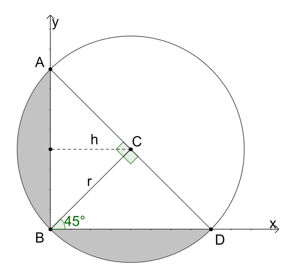
3.4.3. Calculating Various Drone Parameters

One of the prime considerations in drone deployment is that every drone should have the same leftover energy on deployment [18]. In this way, drones nearer to the base stations can be deployed at greater heights to cover the maximum area on the surface.
We use drones with the same battery capacity and initial energy in the proposed method. After a drone is deployed, the leftover energy can be calculated as follows [18]:
e i = B C × ( d i s t i + W × ( h i h b ) ) e i = e j
for 1 ≤ i ≠ j ≤ n, where:
  • h i —the height of the ith drone
  • e i —the leftover energy of the ith drone
  • h b —the height of the base station
  • B—the initial energy of all drones
  • C—the energy parameter (same for all drones)
  • W—the ratio of horizontal lift to drag ratio to vertical lift to drag ratio
  • d i s t i —the horizontal distance travelled by the ith drone
One of our research objectives is to maximize the network coverage of the region. From Equation (1), the maximum leftover energy is obtained when d i s t i = 0 and h i = h m a x . Hence,
e = B C × W ( h m a x h b )
therefore, the maximum leftover energy is obtained when the drone is placed directly above the base station. From Equations (1) and (2), we obtain
B C × W ( h m a x h b ) = B C × ( d i s t i + W × ( h i h b ) ) h i = W × H m a x d i s t i W
For the first drone, d i s t 1 = r 1 , where r 1 is its radius of coverage. Because the coverage region is cone-shaped, r i = h i × t a n α ; therefore,
B C × W ( h m a x h b ) = B C × ( h 1 × t a n α + W × ( h 1 h b ) ) h 1 = W × H m a x W + t a n α
The calculated height value h is adjusted to be within H m i n and H m a x . The radius of coverage is calculated as
r = h × t a n α
where α is the coverage angle of the drone.
Finally, in [18] the authors suggest an equation for finding the leftover energy e in one dimension:
e = B C × d i , d i = | x i x i | + W i × h i
where B is the initial energy of the drone, C is the energy dissipation rate, and x i and x i are the positions of the base station and the drone, respectively. In our case, we have to consider both the Euclidean distance between the base station and the drone and the vertical distance that the drone has traveled ( h h b ). Hence, the above formula converges to
e = B C × ( d i s t + W × ( h h b ) )
where h b is the height of the base station. The height of a deployed drone and its coverage region are shown in Figure 7.
In the above equation, the leftover energy is calculated following the assumption that the terrain is a plane. However, we use a threshold height H m i n (defined in Section 3.3) for practical situations, below which the drone is not deployed. Obviously, this may not guarantee equal leftover energy for every drone, however, the average leftover energy for the entire system is greater than that for a system with drones deployed at equal heights. The procedure is described in Algorithm 1. Note that we fix the height of a drone to be the value of h f i x e d (for the first two drones where h f i x e d 0 ) in lines 11 and 12. Otherwise, we check whether the difference between the actual height ( h + h r e f ) computed for the drone and the height of the obstacle ( h t ) is less than h t d ; if it is, we place the drone at a height h t d above the obstacle (line numbers 19 and 20).
Algorithm 1 FindDroneParameters—Calculating the base station (b), height (h), radius of coverage (r), and leftover energy (e) of the drone
     Input: ( x , y )—position of the drone, h r e f —height of reference point, h f i x e d = 0
     Output: b , h , r , e
1:
d i s t 1 x 2 + y 2
2:
d i s t 2 ( x m ) 2 + ( y n ) 2
3:
d i s t M i n i m u m ( d i s t 1 , d i s t 2 )
4:
if  d i s t = d i s t 1  then
5:
     b 0
6:
     h b H 0 , 0
7:
else
8:
     b 1
9:
     h b H m , n
10:
end if
11:
if  h f i x e d 0  then
12:
     h h f i x e d
13:
else
14:
     h W × H m a x d i s t W
15:
    if  h < H m i n  then
16:
         h H m i n
17:
    end if
18:
     h t H x , y
19:
    if  ( h + h r e f h t ) < h t d  then
20:
         h h t + h t d h r e f
21:
    end if
22:
end if
23:
r tan ( α ) × h
24:
h s m a l l S H x , y , r
25:
if  h + h r e f h s m a l l > H m a x  then
26:
     h H m a x + h s m a l l h r e f
27:
     P e r f o r m 16 t o 18
28:
end if
29:
r tan ( α ) × h
30:
e B C × ( d i s t + W × ( h h b ) )
31:
return ( b , h , r , e )
We try to cover the entire rectangular region with coverage circles of drones from the first base station to the second. We use a layered approach in which each layer consists of a starting circle, a set of circles along the x-direction, and a set of circles along the y-direction. The initial starting circle is placed near the base station at (0, 0).

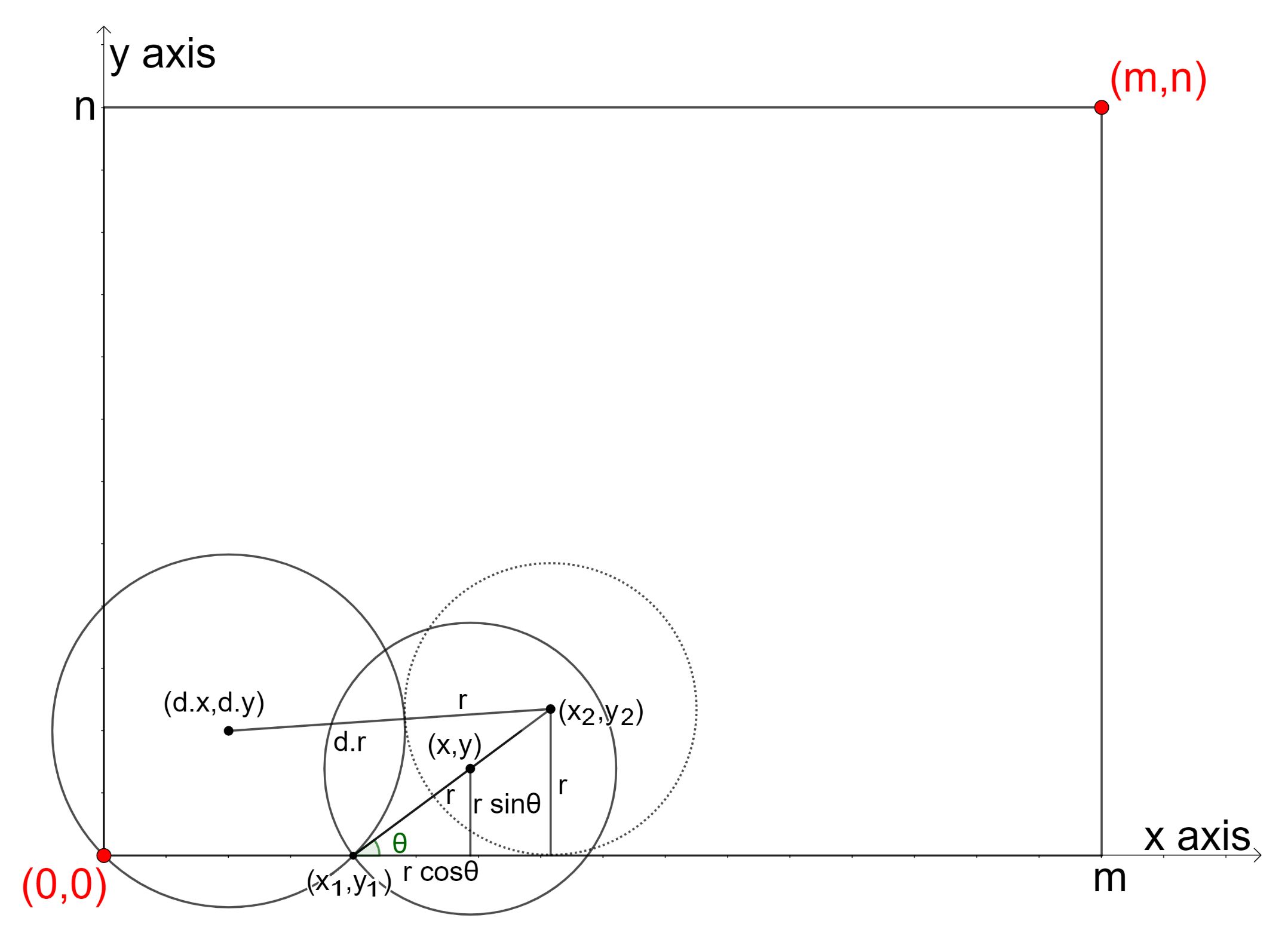
3.4.4. Filling the Coverage Circles along the X and Y Axes

Figure 8 shows how we find circles to be filled along the x-axis. The initial circle near the base station (0, 0) is placed to pass through (0, 0). The value of d for the initial drone is the coverage radius.
The center of the initial circle ( d . x , d . y ) is placed such that the angle made by the line between ( d . x , d . y ) and (0, 0) and the x-axis is 45 , meaning that any wasted coverage is equally distributed along both the x and y directions. The point at which the circle meets the x-axis is marked as ( x 1 , y 1 ). To find the next circle in the x-direction, we assume that it has the same radius (r) as the initial circle and grazes the x-axis. In the figure, its center is ( x 2 , y 2 ). In order to distribute the wastage equally in both directions, we fix the center of the new circle at ( x , y ) at a distance r from ( x 1 , y 1 ) along the angle ( θ ), obtaining a new center and radius for the new circle at ( x , y ). We refine the new circle again with respect to the new center and new radius. This procedure continues until the center in the previous round and that in the current round match. This is analogous to the rounds of the k-means clustering algorithm [43]. The detailed method used for filling circles along the x-axis is provided in Algorithm 2.
The algorithm uses two functions, ArbitraryDistant and EquiDistant. The former finds a point (x, y) at a distance r 1 + r from ( x , y ) and at a distance r 2 + r from ( x , y ), where ( x , y ) and ( x , y ) are any two points and r 1 , r 2 , and r are arbitrary. There may be two different points for ( x , y ) on a plane; in order to always choose the point inside the rectangle, we use a separate variable special in the algorithm. The latter (EquiDistant) fixes the position of a drone object at an equal distance from the positions provided by the parameter points.
Algorithm 2 FillAlongXAxis—Filling drone coverage circles along x-axis
     Input: d—a drone object representing the starting circle of the outer layer
     Output: updated D—collection of drones, updated y r e f —reference y-coordinate for x direction filling.
1:
i n d i c a t i o n E q u i D i s t a n t ( d , { ( 0 , 0 ) , ( m , 0 ) } , 0 )
2:
while  i n d i c a t i o n = 1  do
3:
     r d . r
4:
     x 1 d . x + d . r 2 d . y 2 , y 1 0
5:
     h r e f H x 1 , y 1
6:
     d . h r e f M a x i m u m ( d . h r e f , h r e f )
7:
     ( d . b , d . h , d . r , d . e ) F i n d D r o n e P a r a m e t e r s ( d . x , d . y , d . h r e f )
8:
     x 2 d . x + ( d . r + r ) 2 ( r d . y ) 2 , y 2 r
9:
     θ t a n 1 y 2 y 1 x 2 x 1
10:
     x x 1 + r × c o s θ , y y 1 + r × s i n θ
11:
     ( b , h , r , e ) F i n d D r o n e P a r a m e t e r s ( x , y , h r e f )
12:
     P e r f o r m 8 t o 10
13:
     c o o r d i n a t e s { ( x , y ) }
14:
    while  t r u e  do
15:
         ( b , h , r , e ) F i n d D r o n e P a r a m e t e r s ( x , y , h r e f )
16:
         P e r f o r m s t e p s 8 t o 10
17:
        if  ( x , y ) ϵ c o o r d i n a t e s  then
18:
            ( b 1 , h 1 , r 1 , e 1 ) F i n d D r o n e P a r a m e t e r s ( x , y , h r e f )
19:
           while  h 1 > h  do
20:
                ( b , h , r , e ) ( b 1 , h 1 , r 1 , e 1 )
21:
                P e r f o r m s t e p s 8 t o 10
22:
                ( b 1 , h 1 , r 1 , e 1 ) F i n d D r o n e P a r a m e t e r s ( x , y , h r e f )
23:
           end while
24:
            break
25:
        end if
26:
         c o o r d i n a t e s c o o r d i n a t e s { ( x , y ) }
27:
    end while
28:
     d 1 D r o n e ( x , y , r , h , b , e , h r e f )
29:
     d . e a s t d 1 , d 1 . w e s t d
30:
     D D { d 1 }
31:
     d d 1
32:
     ( x , y ) A r b i t r a r y D i s t a n t ( x 1 , y 1 , m , 0 , 0 , 0 , r )
33:
    if  ( x , y ) a r e d e f i n e d  then
34:
         i n d i c a t i o n 0
35:
    else
36:
         i n d i c a t i o n 1
37:
    end if
38:
end while
39:
i n d i c a t i o n E q u i D i s t a n t ( d , { ( x 1 , y 1 ) , ( m , 0 ) } , 0 )
40:
y r e f d . y + d . r 2 ( m d . x ) 2
We continue the process of finding new circles as long as it is possible to set the center of the new circle equidistant from the points ( x 1 , y 1 ) and ( m , 0 ). The final output of filling along the x-axis is shown in Figure 9.
Filling the circles along the y-axis (FillAlongYAxis) is quite similar to the procedure described above. The only difference is the change in direction, as shown in Figure 10.

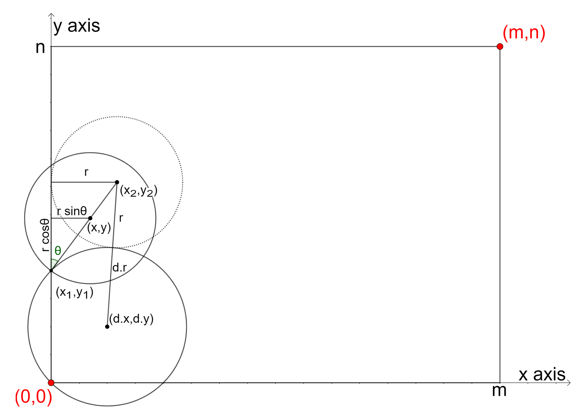
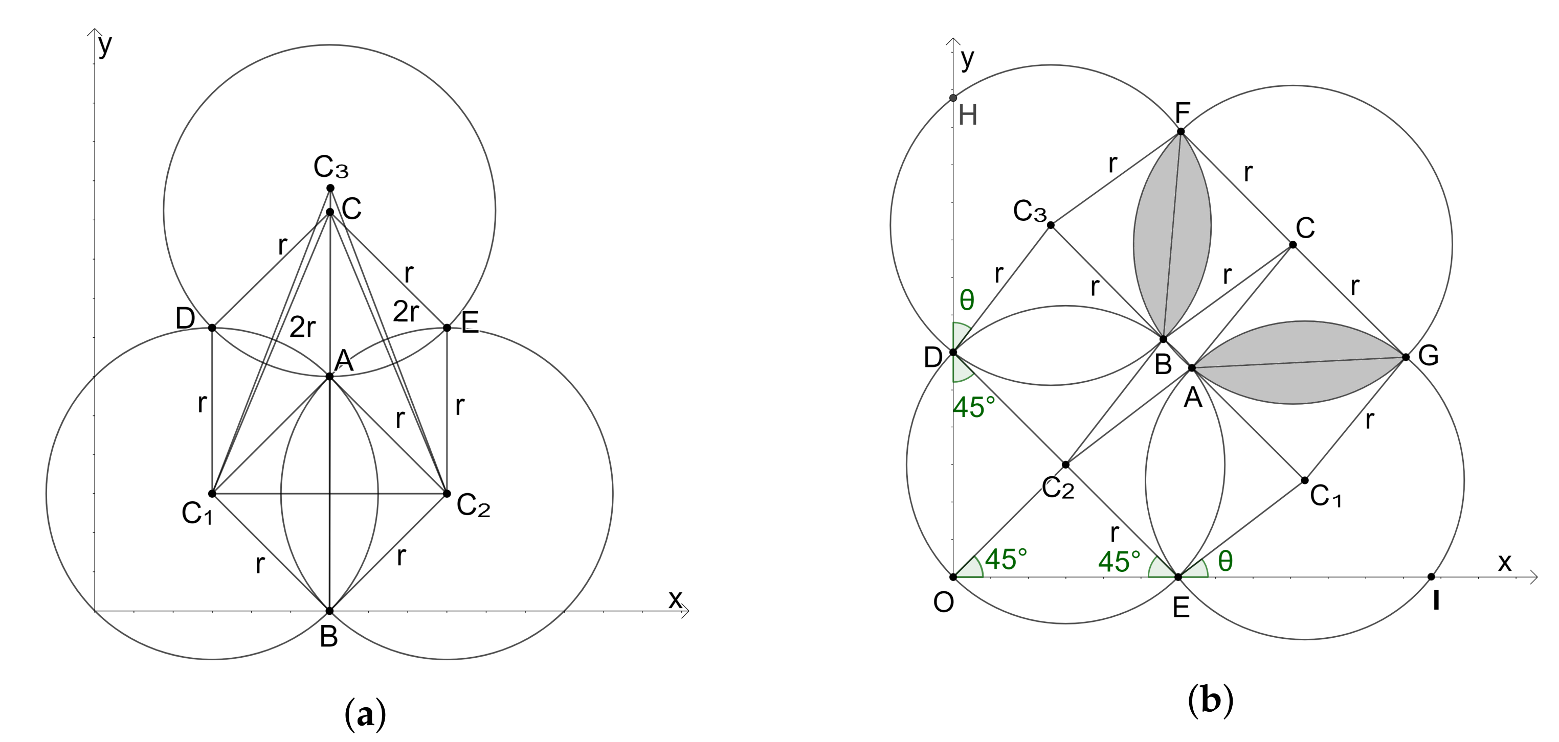
3.4.5. Inner Layer Filling

Having obtained an outer layer of coverage circles along the x and y axes, we now concentrate on the inner layers. We introduce the concept of TwoNeighbours and ThreeNeighbours. TwoNeighbours is the procedure by which we find the center and radius of a circle based on its two neighbours, as shown in Figure 11a, where we find ( x , y ) and r based on the parameters of its neighbouring two circles.
The working of TwoNeighbours is similar to that of the algorithms for filling circles along the x and y axes. We choose a point ( x 2 , y 2 ) at a distance d 1 . r + r from ( d 1 . x , d 1 . y ) and d 2 . r + r from ( d 2 . x , d 2 . y ). Because the value of r is initially unknown, it is chosen as the average of d 1 . r and d 2 . r . We find the center of the new circle ( x , y ) at an angle θ along the line between ( x 1 , y 1 ) and ( x 2 , y 2 ) at a distance r from ( x 1 , y 1 ). We continue to change the values of ( x 2 , y 2 ) and ( x , y ) (a similar situation as in algorithm FillAlongXAxis) until we do not obtain a new point for ( x , y ). The detailed algorithm is shown in Algorithm 3.
Algorithm 3 TwoNeighbours—Calculating the position of a third drone object based on the positions of its two neighbours
     Input: d 1 , d 2 —two neighbouring drone objects
     Output: d—new drone object
1:
if  d 1 | | d 2 n o t d e f i n e d  then
2:
     d n o t d e f i n e d
3:
else
4:
     r A v e r a g e ( d 1 . r , d 2 . r )
5:
     ( x 1 , y 1 ) A r b i t r a r y D i s t a n t ( d 1 . x , d 1 . y , d 2 . x , d 2 . y , d 1 . r , d 2 . r , 0 )
6:
     h r e f H x 1 , y 1
7:
     d 1 . h r e f M a x i m u m ( d 1 . h r e f , h r e f )
8:
     ( d 1 . b , d 1 . h , d 1 . r , d 1 . e ) F i n d D r o n e P a r a m e t e r s ( d 1 . x , d 1 . y , d 1 . h r e f )
9:
     d 2 . h r e f M a x i m u m ( d 2 . h r e f , h r e f )
10:
     ( d 2 . b , d 2 . h , d 2 . r , d 2 . e ) F i n d D r o n e P a r a m e t e r s ( d 2 . x , d 2 . y , d 2 . h r e f )
11:
     P e r f o r m s t e p s 4 a n d 5
12:
     ( x 2 , y 2 ) A r b i t r a r y D i s t a n t ( d 1 . x , d 1 . y , d 2 . x , d 2 . y , d 1 . r , d 2 . r , r )
13:
    if  x 2 = x 1  then
14:
         θ 90
15:
    else
16:
         θ t a n 1 y 2 y 1 x 2 x 1
17:
    end if
18:
     x x 1 + r × c o s θ , y y 1 + r × s i n θ
19:
     ( b , h , r , e ) F i n d D r o n e P a r a m e t e r s ( x , y , h r e f )
20:
     P e r f o r m s t e p s 12 t o 18
21:
     c o o r d i n a t e s { ( x , y ) }
22:
    while  t r u e  do
23:
         P e r f o r m s t e p s 12 t o 19
24:
        if  ( x , y ) ϵ c o o r d i n a t e s  then
25:
            b 1 , h 1 , r 1 , e 1 F i n d D r o n e P a r a m e t e r s ( x , y , h r e f )
26:
           while  h 1 > h  do
27:
                ( b , h , r , e ) b 1 , h 1 , r 1 , e 1
28:
                P e r f o r m s t e p s 12 t o 18
29:
                ( b 1 , h 1 , r 1 , e 1 ) F i n d D r o n e P a r a m e t e r s ( x , y , h r e f )
30:
           end while
31:
            break
32:
        end if
33:
         c o o r d i n a t e s c o o r d i n a t e s { ( x , y ) }
34:
    end while
35:
     d D r o n e ( x , y , r , h , b , e , h r e f )
36:
     d 1 . e a s t d 2 . n o r t h d
37:
     d . w e s t d 1 , d . s o u t h d 2
38:
end if
39:
return d
The concept of ThreeNeighbours is simpler than that of TwoNeighbours, as we have a specific point ( x , y ), as shown in Figure 11b; here, ( x 1 , y 1 ) is a point at a distance r from both ( x 1 , y 1 ) and ( x 2 , y 2 ). The value of r is the average radii of all three neighbouring circles.
We find each circle in the inner layers based on the TwoNeighbours and ThreeNeighbours concepts. Wherever possible, we use ThreeNeighbours, as it is easier to process. The detailed algorithm used for inner x-direction filling is provided in Algorithm 4 (Filling along the y-axis follows a similar procedure). Figure 12 shows the output after filling the inner layers in both the x and y directions.
Algorithm 4 InnerXDirectionFilling—Filling inner layer along the x direction
     Input: d—a drone object that represents the starting circle of the inner layer
     Output: updated D—collection of drones, updated y r e f —reference y—coordinate for x direction filling.
1:
i n d i c a t i o n 1
2:
while  i n d i c a t i o n = 1  do
3:
     d 1 d . s o u t h , d 2 d 1 . e a s t
4:
     ( x 1 , y 1 ) A r b i t r a r y D i s t a n t ( d . x , d . y , d 1 . x , d 1 . y , d . r , d 1 . r , 0 )
5:
     ( x 2 , y 2 ) n o t d e f i n e d
6:
    if  d 2 i s n o t d e f i n e d  then
7:
         d 3 T w o N e i g h b o u r s ( d , d 1 )
8:
    else
9:
        if  ( d 2 . x d . x ) 2 + ( d 2 . y d . y ) 2 d 2 . r + d . r  then
10:
            d 1 d 2 , d 2 d 1 . e a s t
11:
            ( x 1 , y 1 ) A r b i t r a r y D i s t a n t ( d . x , d . y , d 1 . x , d 1 . y , d . r , d 1 . r , 0 )
12:
        end if
13:
         d 3 T h r e e N e i g h b o u r s ( d , d 1 , d 2 )
14:
        if  d 3 i s n o t d e f i n e d  then
15:
            d 3 T w o N e i g h b o u r s ( d , d 1 )
16:
        else
17:
            ( x 2 , y 2 ) A r b i t r a r y D i s t a n t ( d 1 . x , d 1 . y , d 2 . x , d 2 . y , d 1 . r , d 2 . r , 0 )
18:
        end if
19:
    end if
20:
     D D { d 3 } , d d 3
21:
     ( x , y ) A r b i t r a r y D i s t a n t ( x 1 , y 1 , m , y r e f , 0 , 0 , d . r )
22:
    if  ( x , y ) a n d ( x 2 , y 2 ) a r e d e f i n e d  then
23:
        if  ( x 2 x ) 2 + ( y 2 y ) 2 > d . r 2  then
24:
            ( x , y ) A r b i t r a r y D i s t a n t ( x 2 , y 2 , m , y r e f , 0 , 0 , d . r )
25:
        end if
26:
    end if
27:
    if  ( x , y ) a r e d e f i n e d  then
28:
         i n d i c a t i o n 0
29:
    else
30:
         i n d i c a t i o n 1
31:
    end if
32:
end while
33:
if  ( x 2 , y 2 ) a r e d e f i n e d  then
34:
     i n d i c a t i o n E q u i D i s t a n t ( d , { ( x 1 , y 1 ) , ( m , y r e f ) , ( x 2 , y 2 ) } , 0 )
35:
else
36:
     i n d i c a t i o n E q u i D i s t a n t ( d , { ( x 1 , y 1 ) , ( m , y r e f ) } , 0 )
37:
end if
38:
d 1 D [2]
39:
if  ( d 1 . x d . x ) 2 + ( d 1 . y d . y ) 2 d 1 . r + d . r  then
40:
     x 3 m , y 3 d 1 . y d 1 . r 2 ( m d 1 . x ) 2
41:
     ( x , y , r , h , b , e , h r e f ) ( d . x , d . y , d . r , d . h , d . b , d . e , d . h r e f )
42:
     i n d i c a t i o n E q u i D i s t a n t ( d , { ( x 3 , y 3 ) , ( m , y r e f ) } , 1 )
43:
    if i n d i c a t i o n = 0 then
44:
      if x 1 d . x 2 + y 1 d . y 2 > d . r 2   or   x 2 , y 2   are   defined   and   x 2 d . x 2 + y 2 d . y 2 > d . r 2 then
45:
             ( d . x , d . y , d . r , d . h , d . b , d . e , d . h r e f ) ( x , y , r , h , b , e , h r e f )
46:
      end if
47:
   end if
48:
end if
49:
y r e f d . y + d . r 2 ( m d . x ) 2

3.4.6. The Region-Filling Algorithm

The algorithm fixes coverage circles for the base stations at (0, 0) and ( m , n ), as shown in Figure 13, in order to utilize the maximum possible heights for the drones near the base stations. We proceed by filling the circles along the x and y axes. We then move to the inner layer filling to cover the entire region. The detailed procedure is provided in Algorithm 5. The above method uses the minimum number of drones possible.
Algorithm 5 Region Filling
     Input: m , n , H , S H , α , B , W , C , H m a x , H m i n , h t d
     Output: O r d e r e d c o l l e c t i o n o f d r o n e o b j e c t s D
1:
D { } , h W × H m a x d W + tan ( α ) , r h × tan ( α )
2:
x r 2 , y r 2
3:
h b 1 H 0 , 0 , h b 2 H m , n
4:
( b , h 1 , r , e ) F i n d D r o n e P a r a m e t e r s ( x , y , h b 1 , h )
5:
x r 2 , y r 2
6:
d D r o n e ( x , y , r , h 1 , b , e , h b 1 )
7:
c o o r d i n a t e s { }
8:
while  ( d . x , d . y ) c o o r d i n a t e s  do
9:
     c o o r d i n a t e s c o o r d i n a t e s ( d . x , d . y )
10:
     ( d . b , d . h , d . r , d . e ) F i n d D r o n e P a r a m e t e r s ( d . x , d . y , d . h , d . h r e f )
11:
     d . x r 2 , d . y r 2
12:
end while
13:
D D { d }
14:
if  ( d . x m ) 2 + ( d . y n ) 2 > d . r 2  then
15:
     ( b , h 1 , r , e ) F i n d D r o n e P a r a m e t e r s ( m d . x , n d . y , h b 2 , h )
16:
     x m r 2 , y n r 2
17:
     d 1 D r o n e ( x , y , r , h 1 , b , e , h b 2 )
18:
     c o o r d i n a t e s { }
19:
    while  ( d 1 . x , d 1 . y ) c o o r d i n a t e s  do
20:
         c o o r d i n a t e s c o o r d i n a t e s { ( d 1 . x , d 1 . y ) }
21:
         ( d 1 . b , d 1 . h , d 1 . r , d 1 . e ) F i n d D r o n e P a r a m e t e r s ( d 1 . x , d 1 . y , d 1 . h , d 1 . h r e f )
22:
         d 1 . x m d 1 . r 2 , d 1 . y n d 1 . r 2
23:
    end while
24:
     D D { d 1 }
25:
     ( x 1 , y 1 ) A r b i t r a r y D i s t a n t ( d . x , d . y , d 1 . x , d 1 . y , d . r , d 1 . r , 0 )
26:
     ( x 2 , y 2 ) A r b i t r a r y D i s t a n t ( d . x , d . y , d 1 . x , d 1 . y , d . r , d 1 . r , 0 , 1 )
27:
    if  ( x 1 , y 1 ) a r e n o t d e f i n e d o r , ( x 1 , y 1 ) a r e d e f i n e d a n d M a x i m u m ( y 1 , y 2 ) < n o r M i n i m u m ( y 1 , y 2 ) > 0  then
28:
         F i l l A l o n g X a x i s ( d )
29:
         F i l l A l o n g Y a x i s ( d )
30:
        while  t r u e  do
31:
            d 1 d . n o r t h , d 2 d . e a s t
32:
           if  d 1 o r d 2 i s n o t d e f i n e d  then
33:
                break
34:
           end if
35:
            ( x 1 , y 1 ) ( x 2 , y 2 ) n o t d e f i n e d
36:
           if  ( d 1 . x d 2 . x ) 2 + ( d 1 . y d 2 . y ) 2 d 1 . r + d 2 . r  then
37:
                d 3 T w o N e i g h b o u r s ( d 1 , d 2 )
38:
                ( x 1 , y 1 ) A r b i t r a r y D i s t a n t ( d 1 . x , d 1 . y , d 2 . x , d 2 . y , d 1 . r , d 2 . r , 0 )
39:
           else
40:
                d 3 T h r e e N e i g h b o u r s ( d 1 , d , d 2 )
41:
               if  d 3 i s n o t d e f i n e d  then
42:
                    d 4 T w o N e i g h b o u r s ( d 1 , d 2 )
43:
                    d 5 T w o N e i g h b o u r s ( d , d 2 )
44:
                    D D { d 4 , d 5 }
45:
                    I n n e r X D i r e c t i o n F i l l i n g ( d 5 )
46:
                    I n n e r Y D i r e c t i o n F i l l i n g ( d 4 )
47:
                    continue
48:
               else
49:
                   ( x 1 , y 1 ) A r b i t r a r y D i s t a n t ( d 1 . x , d 1 . y , d . x , d . y , d 1 . r , d . r , 0 )
50:
                   ( x 2 , y 2 ) A r b i t r a r y D i s t a n t ( d . x , d . y , d 2 . x , d 2 . y , d . r , d 2 . r , 0 )
51:
           end if
52:
         end if
53:
           if  ( d 3 . x m ) 2 + ( d 3 . y n ) 2 d 3 . r 2  then
54:
                break
55:
           end if
56:
            D D { d 3 }
57:
            d d 3
58:
            d 1 D { 2 } , d 2 d . s o u t h , d 3 d . w e s t
59:
           if  ( ( d 1 . x d . x ) 2 + ( d 1 . y d . y ) 2 d 1 . r + d . r ) a n d ( d 2 . x + d 2 . r m o r d 3 . y + d 3 . r n )  then
60:
               if  d 2 . x + d 2 . r m  then
61:
                    x 3 x 4 m
62:
                    y 3 d 2 . y + d 2 . r 2 ( m d 2 . x ) 2
63:
                    y 4 d 1 . y + d 1 . r 2 ( m d 1 . x ) 2
64:
                    ( x , y , r , h , b , e , h r e f ) ( d . x , d . y , d . r , d . h , d . b , d . e , d . h r e f )
65:
                    i n d i c a t i o n E q u i D i s t a n t ( d , { ( x 3 , y 3 ) , ( x 4 , y 4 ) } , 1 )
66:
                   if  i n d i c a t i o n = 0  then
67:
                       if  ( ( x 1 d . x ) 2 + ( y 1 d . y ) 2 > d . r 2 ) o r ( x 2 , y 2 ) a r e d e f i n e d a n d ( x 2 d . x ) 2 + ( y 2 d . y ) 2 > d . r 2 )  then
68:
                           ( d . x , d . y , d . r , d . h , d . b , d . e , d . h r e f ) ( x , y , r , h , b , e , h r e f )
69:
                       end if
70:
                   else
71:
                        break
72:
                   end if
73:
               end if
74:
           else if  d 3 . y + d 3 . r n  then
75:
                x 3 d 3 . x + d 3 . r 2 ( n d 3 . y ) 2
76:
                x 4 d 1 . x + d 1 . r 2 ( n d 1 . y ) 2
77:
                y 3 y 4 n
78:
                ( x , y , r , h , b , e , h r e f ) ( d . x , d . y , d . r , d . h , d . b , d . e , d . h r e f )
79:
                i n d i c a t i o n E q u i D i s t a n t ( d , { ( x 3 , y 3 ) , ( x 4 , y 4 ) } , 1 )
80:
               if  i n d i c a t i o n = 0  then
81:
                   if  ( ( x 1 d . x ) 2 + ( y 1 d . y ) 2 > d . r 2 ) o r ( x 2 , y 2 a r e d e f i n e d a n d ( x 2 d . x ) 2 + ( y 2 d . y ) 2 > d . r 2 )  then
82:
                        ( d . x , d . y , d . r , d . h , d . b , d . e , d . h r e f ) ( x , y , r , h , b , e , h r e f )
83:
                   end if
84:
               else
85:
                    break
86:
               end if
87:
           else if  d 2 . x + d 2 . r m  then
88:
                x 3 m
89:
                y 3 d 2 . y + d 2 . r 2 ( m d 2 . x ) 2
90:
               if  ( x 2 , y 2 ) a r e d e f i n e d  then
91:
                    i n d i c a t i o n E q u i D i s t a n t ( d , { ( x 1 , y 1 ) , ( x 3 , y 3 ) , ( x 2 , y 2 ) } , 0 )
92:
               else
93:
                    i n d i c a t i o n E q u i D i s t a n t ( d , { ( x 1 , y 1 ) , ( x 3 , y 3 ) } , 0 )
94:
               end if
95:
               if  i n d i c a t i o n = 0  then
96:
                    I n n e r Y D i r e c t i o n F i l l i n g ( d )
97:
                    break
98:
               end if
99:
           else if  d 3 . y + d 3 . r n  then
100:
                x 3 d 2 . x + d 2 . r 2 ( n d 2 . y ) 2
101:
                y 3 n
102:
               if  ( x 2 , y 2 ) a r e d e f i n e d  then
103:
                    i n d i c a t i o n E q u i D i s t a n t ( d , { ( x 1 , y 1 ) , ( x 3 , y 3 ) , ( x 2 , y 2 ) } , 0 )
104:
               else
105:
                    i n d i c a t i o n E q u i D i s t a n t ( d , { ( x 1 , y 1 ) , ( x 3 , y 3 ) } , 0 )
106:
               end if
107:
               if  i n d i c a t i o n = 0  then
108:
                    I n n e r X D i r e c t i o n F i l l i n g ( d )
109:
                    break
110:
               end if
111:
           end if
112:
            I n n e r X D i r e c t i o n F i l l i n g ( d )
113:
            I n n e r Y D i r e c t i o n F i l l i n g ( d )
114:
           if  ( ( d 1 d . x ) 2 + ( d 1 . y d . y ) 2 d 1 . r + d . r ) o r ( d . x + d . r m o r d . y + d . r n )  then
115:
                break
116:
           end if
117:
        end while
118:
    end if
119:
end if
120:
returnD

3.5. Complexity Analysis of the Region Filling Algorithm

The time complexity of the region-filling algorithm is directly proportional to the number of drones required to cover the region, which is ≈ m × n π r 2 W , where W is the average wastage (defined as W = T o t a l a r e a o f w a s t a g e N u m b e r o f c i r c l e s ) and r is the average radius of a circle. Therefore, the time complexity is T ( n ) = O( m × n π r 2 W )
In the best case,
r = H m a x × t a n α T ( n ) = O ( m × n π ( H m a x × t a n α ) 2 W )
In the worst case,
r = H m i n × t a n α T ( n ) = O ( m × n π ( H m i n × t a n α ) 2 W )
In the average case,
r = ( H m a x + H m i n 2 ) × t a n α T ( n ) = O ( m × n π ( ( H m a x + H m i n 2 ) × t a n α ) 2 W )
where
  • α is the coverage angle
  • H m a x is the maximum possible altitude
  • H m i n is the minimum possible altitude

3.6. Proof That Our Method Uses the Minimum Number of Drones

To prove that the region-filling algorithm uses the minimum number of drones to cover the whole region, we show that the various stages in the algorithm ensure the minimum waste of coverage, and hence the minimum number of drones. The minimum wastage happens when the wastage is distributed equally in all directions.

3.6.1. Deployment of the Initial Drone

A straightforward idea in placing the first (or last) drone is that its coverage boundary should pass through the origin. In order to attain minimum wastage, we use the idea of dividing wastage equally along both axes. Consider a circle with a center C and radius r, as in Figure 14:
A C B = B C D = 90 A r e a ( S e g m e n t A B ) = r 2 ( θ π 360 s i n θ 2 ) = A r e a ( S e g m e n t B D )
hence, the wastage is equally distributed along both axes.

3.6.2. Wastage of Coverage in FillAlongXAxis and FillAlongYAxis

As given in the methods FillAlongXAxis and FillAlongYAxis, the radii of the different circles filling the rectangular region are different when deploying drones along the x and y axes. The boundaries of the rectangular region are then (0, 0) and ( m , n ).
Consider a circle with a center E and radius r 1 , as in Figure 15. We want to find the center C such that the wastage is distributed as equally as possible. For this, we find a point C 1 which is r 1 + r distant from E and at an r vertical distance from the x-axis. Let B be ( x 1 , 0) and C 1 be ( x 2 , r); now, C can be calculated as x = x 1 + r c o s θ and y = r s i n θ . To prove the efficiency of this approach, we can consider r 1 = r, meaning that E is ( r 2 , r 2 ). Therefore,
( x 1 r 2 ) 2 + ( r 2 ) 2 = r 2 x 1 = 2 r
The distance between E and C 1 is r 1 + r = 2 r . Therefore,
( x 2 r 2 ) 2 + ( r r 2 ) 2 = 4 r 2 x 2 = r ( 1 2 + 4 ( 1 1 2 ) 2 ) θ = t a n 1 ( y 2 y 1 x 2 x 1 ) = t a n 1 ( r r ( 4 ( 1 1 2 ) 2 ) 1 2 ) 37 . 008 A C B = 45 + θ = 82 . 008 ( ACBE is a rhombus ) B C D = 180 2 θ = 105 . 984 ( BCD is an isosceles triangle )
2 ( A r e a ( S e g m e n t A B ) ) = 2 ( r 2 ( A C B π 360 s i n ( A C B ) 2 ) ) 0.46 r 2 A r e a ( S e g m e n t B D ) = r 2 ( B C D π 360 s i n ( B C D ) 2 ) 0.42 r 2 2 ( A r e a ( S e g m e n t A B ) ) A r e a ( S e g m e n t B D )
Here, the wastage of coverage (between the x-axis and the circles and between two circles) is distributed almost equally. A similar proof can be shown for the wastage with respect to the y-axis.

3.6.3. Wastage of Coverage in TwoNeighbours

Considering two circles with centers C 1 and C 2 and radii r 1 and r 2 , we want to find the center C and radius r of the third circle such that the wastage is distributed among the two circles proportionally to their areas. To this end, our approach is to find a point C 3 which is r 1 + r distant from C 1 and r 2 + r distant from C 2 , as in Figure 16a.
Let A be the intersecting point of circles with centers C 1 and C 2 near to point C 3 , and let r 1 = r 2 = r. The locus of all points equidistant at an arbitrary distance from points C 1 and C 2 is then a straight line passing through the point of the line joining C 1 and C 2 . Thus, C A B ¯ is a straight line. Here, A C 2 B C 1 , C D C 1 A , and C E C 2 A are each in the shape of a rhombus, while C A C 1 and C A C 2 are congruent.
C 1 C A = C 2 A C ( CPCT ) A C D = 2 C 1 C A = 2 C 2 C A = A C E = θ
A r e a ( S e g m e n t A D ) = r 2 ( π θ 360 s i n θ 2 ) = ( A r e a ( S e g m e n t A E ) ) 2 ( A r e a ( S e g m e n t A D ) ) = 2 ( A r e a ( S e g m e n t A E ) )
Hence, the wastage is equally distributed among the two neighbours.

3.6.4. Wastage of Coverage in ThreeNeighbours

Considering three circles with centers C 1 , C 2 , and C 3 and radii r 1 , r 2 , and r 3 , respectively, we want to find the center of the next circle C with radius r. Let A be the intersecting point of circles with centers C 1 and C 2 and let B be that of circles with centers C 2 and C 3 , as shown in Figure 16b; furthermore, let r 1 = r 2 = r 3 = r.
D C 2 O = E C 2 O = 90 D C 2 E ¯ is a straight line .
it is evident that
D C 2 ¯ C 2 E ¯ C 3 B ¯ A C 1 ¯ and C 3 B A C 1 ¯ is a straight line .
C 3 D H = C 1 E I = θ C 3 D C 2 = C 2 E C 1 = 135 θ 2 C 3 D C 2 + 2 D C 3 B = 360 D C 3 B = 360 2 ( 135 θ ) 2 = 45 + θ C 2 B A = D C 3 B ( Corresponding angles of D C 3 ¯ & C 2 B ¯ ) A B C = C 2 B A ( Property of rhombus C 2 BCA ) B C 3 F = A B C ( Corresponding angles of B C ¯ & C 3 F ¯ ) = 45 + θ 2 ( A r e a ( s e g m e n t B F ) ) = 2 r 2 ( ( 45 + θ ) π 360 s i n ( 45 + θ ) 2 )
Similarly,
2 ( A r e a ( s e g m e n t G A ) ) = 2 r 2 ( ( 45 + θ ) π 360 s i n ( 45 + θ ) 2 ) 2 ( A r e a ( s e g m e n t B F ) ) = 2 ( A r e a ( s e g m e n t G A ) )
hence, the wastage of the area of the circle centered at C is equally distributed among those centered at C 1 and C 3 .

3.6.5. Wastage of Coverage in InnerXDirectionFilling and InnerYDirectionFilling

Both InnerXDirectionFilling and InnerYDirectionFilling make use of ThreeNeighbours and TwoNeighbours. The last circle’s center along each round of InnerXDirectionFilling is set to be equidistant from ( m , y r e f ) and another reference point of the circle. Similarly, for InnerYDirectionFilling, the last circle’s center is set to be equidistant from ( x r e f , n ) and another reference point of the circle. The reason for this is to focus on the circular area within the target region. Because TwoNeighbours and ThreeNeighbours are proven to equally distribute the wastage area, their combination minimizes the required number of drones.

3.6.6. The Region Filling-Algorithm Minimizes the Number of Drones Required

After filling the first layer, the starting circle of the next layer is filled using ThreeNeighbours, followed by filling along the inner x-direction and y-direction. This process continues until the stopping condition is met. As it is proven that the procedures used by the region-filling algorithm distribute wastage of coverage equally and minimize the required number of drones, the combination of these procedures results in the minimum number of drones.

4. Experiments and Results

We conducted various experiments using the terrain data of the landslide-affected region of Pettimudi, Kerala, India, for drone deployment to establish communication. We considered homogeneous drones with similar parameters. The various parameters we used (environmental and drone specific) are shown in Table 2 and Table 3.
We fix H m a x as 2 km. The disaster affected area of Pettimudi is obtained from Google Maps. We consider base stations at diagonally opposite corners, with the first at (9.9913888888888, 76.9316666666667) and the second at (10.0275000000002, 76.96833333333339). We fetch the altitude data of the region using the Google Elevation API. The DMS format is first converted to DD format, then the coordinates are converted to UTM. The altitudes from the API are measured from sea level. To convert the altitude data to heights with reference to the lowest point in the terrain under consideration, we subtract the altitude of the lowest point from each point in the altitude data in order to obtain the normalized altitudes, which are used to populate the data structure HeightMatrix (H). We use the altitude of the nearest point in the matrix for missing altitude data of any point.
We apply the region-filling algorithm for the area and obtain the coverage and drone positions, as shown in Figure 17. It is found that sixteen drones are needed to cover the region effectively. The various parameters, specific to Pettimudi, found are shown in Table A1 of Appendix A.

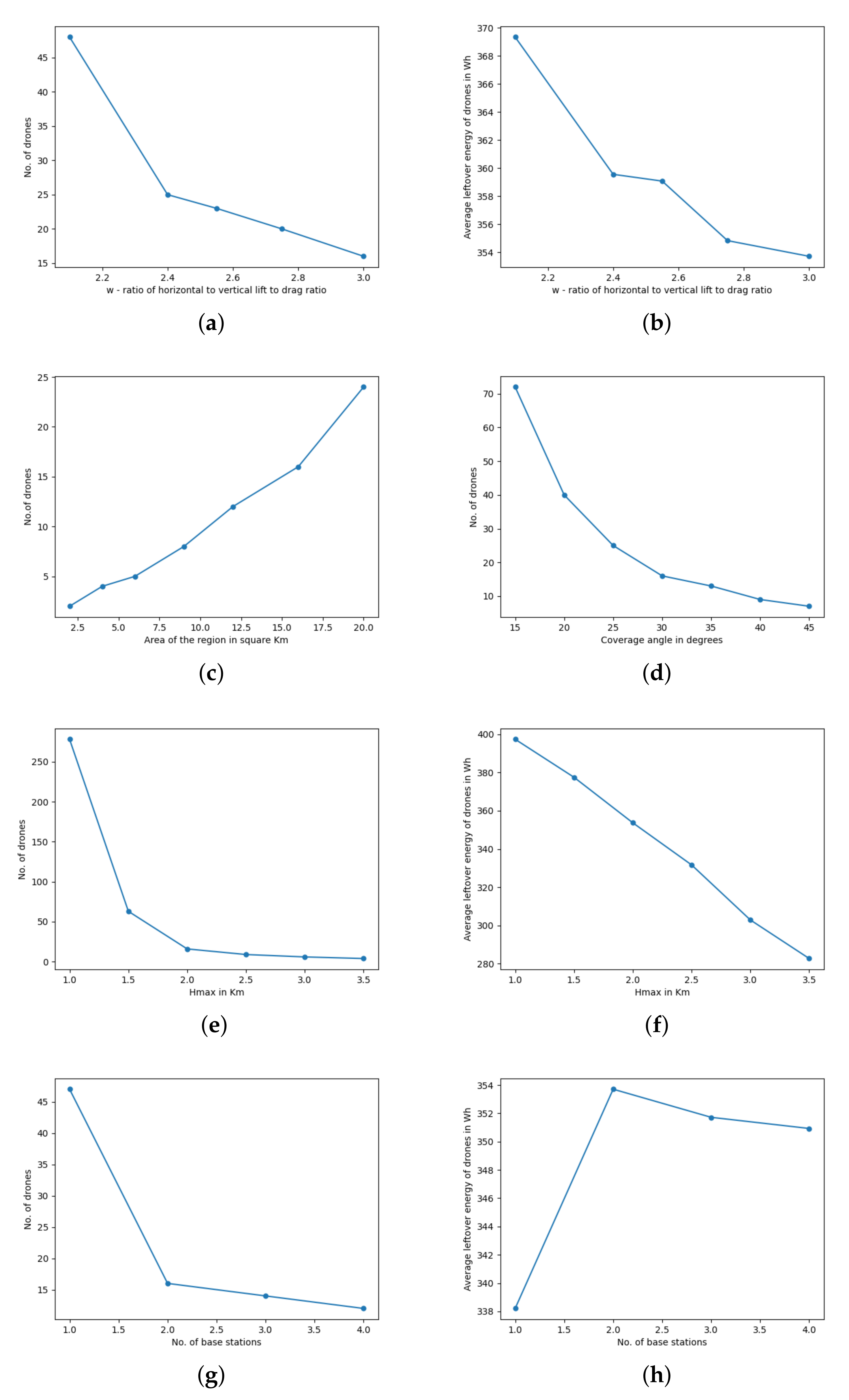
4.1. Analysis of Results

In this section, we show how the double optimization problem (minimizing the number of drones and maximizing the average leftover energy) is addressed. We plot the relation between various drone parameters, as in Figure 18.

4.1.1. Ratio of Horizontal Lift to Drag Ratio to Vertical Lift to Drag Ratio (W)

We attempt to obtain the change in the number of drones required for covering the area with varying values of ratio of horizontal lift to drag ratio to vertical lift to drag ratio (W). Our experiments show the graph as in Figure 18a. We obtain another plot of W vs. average leftover energy, shown in Figure 18b. We observe that the number of drones required decreases with an increase in the value of W. However, the average leftover energy decreases with increasing W. Hence, choosing a value of W is a double optimization problem, and the result can be obtained using the elbow method. A value of W = 2.4 is the most optimal in our experiments.

4.1.2. Area of the Region

It is interesting to see how the area of the region affects the number of drones required. Our experiments yield the plot shown in Figure 18c. The graph shows a linear relationship with the parameters.

4.1.3. Coverage Angle

The coverage angle ( α ) is a parameter of the drone that determines the area where a drone can facilitate effective communication. Our analysis shows that an increase in coverage angle reduces the number of drones required. However, this relationship is only sublinear, as shown in Figure 18d.

4.1.4. Maximum Height ( H M a x )

H m a x is the maximum attainable height for a drone with sufficient network strength. The graph in Figure 18e suggests that the number of drones decreases exponentially with increasing H m a x , while the plot in Figure 18f shows the linear relationship between H m a x and the average leftover energy. These two plots again lead to a double optimization and, in our case, the optimal value for H m a x is 2 km.

4.1.5. Number of Base Stations
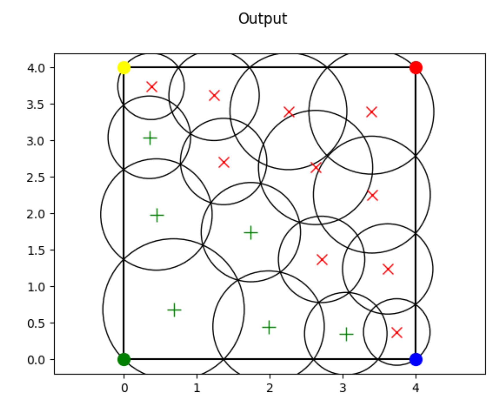
For a rectangular disaster affected area, the base stations can be placed only in the corners, as ground-level access inside the terrain may not be possible. Therefore, the number of base stations can be one, two, three, or four. Figure 18g shows the relationship between the number of drones required to cover the region and the number of base stations used. From the graph, we can see that the number of drones required decreases with an increasing number of base stations. We then compare the average leftover energy with the number of base stations; the graph is shown in Figure 18h. The curves in these two plots lead towards the solution of a double optimization problem (maximizing the average leftover energy while at the same time minimizing the number of drones required), and in our case, a value of two for the number of base stations is found to be optimal.
We further consider the corners at which the base stations can be placed. They can be placed either in adjacent corners or diagonally opposite to each other. As explained in the description of the region-filling algorithm, the first base station is always placed at (0, 0). A plot showing H m a x vs. the number of drones required when the second base station is placed at various corners is shown in Figure 19a. A similar plot for the average leftover energy is shown in Figure 19b. These plots suggest that placing the second base station diagonally opposite to the first yields the maximum efficiency.

4.2. Simulation

We simulated drone deployment for the Pettimudi region using Matlab and OMNet++ [44]. OMNeT++ is a discrete event simulator mainly used for network simulation. We used the INET Framework in OMNet++ to simulate the wireless networks.
The terrain data of Pettimudi region (4 km × 4 km) were obtained using the Google Elevation API. A simulation of the terrain is shown in Figure 20a. After construction of the Height Matrix data structure, the region-filling algorithm produces the positions of the sixteen drones deployed to cover the entire area. The drones are deployed using two base stations placed at two diagonally opposite corners of the rectangular region. The trajectories of the drones deployed from the base stations is shown in Figure 20b. After the drones reach their specified coordinates based on the output from the region-filling algorithm, the communications network is established. Here, we take 30 as the coverage angle ( α ). The network coverage obtained is shown in Figure 20b. Figure 21a shows the cone-shaped network coverage of the sixteen deployed drones. Figure 21b shows a top view of the network coverage. It can be observed that the region is fully covered, with no voids in between. The altitudes at which different drones are placed is shown in Figure A1 of Appendix A.
The simulation process proceeds as follows. The terrain map of Pettimudi is generated using the OsgEarth package provided in OMNeT++. The entire 4 km x 4 km is divided into sixteen equal-area rectangles. A cell phone is placed at each of these rectangles and each cell phone is constrained to move inside these rectangles randomly to cover different points in the region. During these movements, the cell phone can send a UDP packet to the nearest drone host. Our simulation shows an average network efficiency (percentage ratio of the number of packets received to the number of packets sent) of 98%.
The simulation videos are available in supplementary materials. The simulation results confirm that the terrain-aware nature of the region-filling algorithm ensures that every cell phone inside the region is covered by the network.

5. Discussions

The strategy of establishing a communications network without any voids by deploying drones in disaster affected areas at optimal heights with a view to minimizing the number of drones and maximizing the average leftover energy is a unique approach. In this section, we compare our approach with other methods available in the literature which are closely related.
Ullah et al. [8] presented an idea for a bush fire mitigation system using drones, specifically, for the 2019–2020 bush fires in New South Wales, Australia. Using a swarm of drones to monitor the bush fire, they developed a method based on PSO to obtain the shortest path a drone has to travel to the target area, thereby ensuring that it uses the maximum hovering time and the minimum travel time. The drone travels back to the sink station after the monitoring is over. Here, our objective is different, as we want to continuously provide communication facilities until the rescue operation is over. Furthermore, we have to ensure that every single point in the affected region is under network coverage, which cannot be guaranteed by the above approach.
Kurt et al. [45] proposed the idea of establishing in-network connectivity between drones used for intelligent traffic management and damage assessment in post-disaster scenarios. They use a connectivity maintenance heuristic that causes changes in the formation of drones in response to the service requests. It focuses on a planar surface, whereas in our case the algorithm considers terrain types with different obstacles at different heights. Furthermore, the above paper does not pay very much attention to energy conservation, while our method focuses on maximizing the average leftover energy by placing the drones at different heights. Moreover, the above method concentrates on connectivity maintenance between drones, while our technique relies on quick establishment of communications between the base stations and end users, with the drones in between, which ensures that there are no network voids in the disaster-struck terrain.

6. Conclusions

Natural calamities such as floods, earthquakes, and landslides are inevitable, and can cause severe damage to human life. With the advent of new technologies, sophisticated mechanisms are available for rescue operations in such situations. One of the major threats that rescue teams face is damage to communication infrastructure, which hinders the progress of rescue due to the difficulties faced in coordination. The easiest method of communication in the present era is by cell phone. However, cell phones are unusable if the base stations providing network coverage are damaged in the calamity. An easy way to establish network coverage for cell phone communications is by hosting base stations in drones. However, drones have limited battery life and may require a substantial amount of energy to fly to their destinations. They have to frequently return to the nearest base station to be recharged, then fly back to their destination. This may introduce voids in network coverage, making rescue operations inefficient. In this paper, we introduce a novel algorithm (the region-filling algorithm) for deploying drones in disaster-affected areas in a way that ensures that there are no voids in coverage and that maximum average leftover energy is available for the network. In addition, we ensure that the algorithm finds a deployment pattern that uses the minimum possible number of drones. We selected Pettimudi, India, a disaster affected location, for simulation experiments to find the drone deployment pattern for the region based on our algorithm. Our experiments show that the algorithm is able to find a drone deployment pattern that provides coverage to the entire area. Furthermore, our approach ensures that the maximum average leftover energy is available for the drones via deployment at different heights while taking the local terrain into consideration. We prove our claim that this approach uses the minimum number of drones, and present a simulation of our algorithm using Matlab and OMNet++.

7. Future Work

Our future work will include experiments with real hardware drones instead of simulations. In addition, we intend to incorporate the following areas into our research:
  • Here, we have considered only perfect circular-shaped coverage for drones; we intend to engage in a detailed exploration of other shapes as well.
  • The present work concentrates on the algorithm used to fill the area without voids using stationary drones. We intend to study the effects of achieving the same using moving drones. In addition, we may explore different technologies available for establishing and maintaining communication between the drones and base stations.
  • A detailed comparison between the region-filling algorithm and other network coverage management methods should be explored.
Finally, we intend to optimize the region-filling algorithm by finding the best specific terrain locations for the base stations.

Supplementary Materials

The following supporting information can be downloaded at: https://www.mdpi.com/article/10.3390/computers11090139/s1, Video S1: 3D simulation of drone deployment in Pettimudi, created in MatLab, Video S2: Simulation of drone deployment in Pettimudi, created in OmNet++.

Author Contributions

Conceptualization, K.M.B.S.K.; methodology, B.V.V., P.S.K. and K.M.B.S.K.; software, B.V.V., P.S.K., R.S.J. and J.T.; validation, B.V.V., P.S.K., R.S.J. and J.T.; formal analysis, B.V.V. and P.S.K.; investigation, R.S.J. and J.T.; resources, K.M.B.S.K.; data curation, R.S.J.; writing—original draft preparation, B.V.V., P.S.K., R.S.J. and J.T.; writing—review and editing, K.M.B.S.K.; visualization, J.T.; supervision, K.M.B.S.K.; project administration, K.M.B.S.K.; funding acquisition, K.M.B.S.K. All authors have read and agreed to the published version of the manuscript.

Funding

This research was funded by TEQIP Phase II of the Rajiv Gandhi Instituite of Technology, Kottayam, India.

Institutional Review Board Statement

Not applicable.

Informed Consent Statement

Not applicable.

Data Availability Statement

Not applicable.

Acknowledgments

The authors would like to thank TEQIP Phase II of the Rajiv Gandhi Institute of Technology, Kottayam, India, for providing financial assistance for this research.

Conflicts of Interest

The authors declare no conflict of interest.

Appendix A. Data on Pettimudi

Table A1 shows the positions, base stations, coverage, leftover energy, and hovering time for each drone for the Pettimudi region, found using the region-filling algorithm. Figure A1 shows the simulation of drones placed at different altitudes and their coverage, highlighting that the drones placed near the base stations are located at greater heights in order to maintain the leftover energy of all the drones as approximately equal.
Table A1. Actual drone positions and other parameters for the Pettimudi region as obtained by the region-filling algorithm.
Cartesian Coordinates ( x , y ) and Normalized Heights in kmReal World Coordinates ( x , y ) and Heights from the Sea Level in kmRadius of Coverage in kmBase StationLeftover Energy in WhHovering Time in Minutes
(0.6850012909668802,
0.6850012909668802,
1.9810872946905196)
(9.9975445782069,
76.93794986634965,
2.52708729469052)
1.1443380310339.29423.38707962
(1.9863072120622192,
0.4500208730417653,
1.6521173291631104)
(9.99535120808547,
76.94980395247727,
2.1981173291631104)
0.9543146820338.0182523.13270969
(3.0440939462526897,
0.35293290321067433,
1.3095049307901139)
(9.994416966351103,
76.9594446404037,
1.855504930790114)
0.7564110370338.0182523.13270969
(3.742788025157351,
0.3762679343689235,
1.0910503229335835)
(9.994590335836122,
76.96581724258051,
1.6370503229335835)
0.6302248181360.4147527.59831517
(0.4500208730417653,
1.9863072120622192,
1.5481173291631105)
(10.009320044652764,
76.93587672010516,
2.0941173291631108)
0.8942410270342.9322524.11250498
(0.35293290321067433,
3.0440939462526897,
1.3035049307901139)
(10.01888693185655,
76.93504800175259,
1.849504930790114)
0.7529452490338.3017523.18923634
(0.3762679343689235,
3.742788025157351,
1.1140503229335836)
(10.025201446811009,
76.93529828116637,
1.6600503229335837)
0.6435103371359.32827.38162967
(1.7439562567843623,
1.7439562567843503,
1.481891136490049)
(10.007060435737923,
76.94766363480579,
2.027891136490049)
0.8559867050339.29423.38707962
(2.7124246028936443,
1.3706564833549857,
1.355107375455865)
(10.003634231219198,
76.95647521198755,
1.901107375455865)
0.7827524361359.044527.32510302
(3.618532811839651,
1.2396785509335047,
1.146148156903163)
(10.00240158709933,
76.96473106479948,
1.6921481569031631)
0.6620510511371.140529.73690682
(1.37065648335483,
2.71242460289361,
1.2411073754558135)
(10.015834661655397,
76.94431150115088,
1.7871073754558136)
0.7169024681364.43128.3991094
(1.239678550933715,
3.61853281183974,
1.3511481569032364)
(10.024032260677686,
76.94316581197926,
1.8971481569032365)
0.7804654681361.4542527.80557956
(2.630328456811882,
2.630328456812093,
1.4423306425423421)
(10.015025145572809,
76.95579474007404,
1.9883306425423422)
0.8331353261370.5262529.61443241
(3.4013205248344214,
2.2585005948062418,
1.63315625474712)
(10.011622647234047,
76.96280560529775,
2.17915625474712)
0.9433621721363.013528.11647614
(2.2585005948064087,
3.4013205248342473,
1.8341562547471535))
(10.02201430185454,
76.95244553872685,
2.3801562547471535)
1.0594660641353.5162526.22283331
(3.395089978241617,
3.395089978241617,
2.0140000000000002)
(10.021896870058129,
76.96281057227907,
2.5600000000000005)
1.163349441360.549066727.62509637
Figure A1. Figure showing the heights at which drones are placed in the simulation.
Computers 11 00139 g0a1

References

  1. Khaled, Z.E.; Mcheick, H. Case studies of communications systems during harsh environments: A review of approaches, weaknesses, and limitations to improve quality of service. Int. J. Distrib. Sens. Netw. 2019, 15, 9960. [Google Scholar] [CrossRef]
  2. Kamruzzaman, M.; Sarkar, N.I.; Gutierrez, J.; Ray, S.K. A study of IoT-based post-disaster management. In Proceedings of the 2017 International Conference on Information Networking (ICOIN), Da Nang, Vietnam, 11–13 January 2017; pp. 406–410. [Google Scholar] [CrossRef]
  3. Lefeuvre, F.; Tanzi, T. About radio science contribution to disaster management. In Proceedings of the 2014 XXXIth URSI General Assembly and Scientific Symposium (URSI GASS), Beijing, China, 16–23 August 2014; pp. 1–4. [Google Scholar] [CrossRef]
  4. Achu, A.L.; Joseph, S.; Aju, C.D.; Mathai, J. Preliminary analysis of a catastrophic landslide event on 6 August 2020 at Pettimudi, Kerala State, India. Landslides 2021, 18, 1459–1463. [Google Scholar] [CrossRef]
  5. Krishnakumar, G.; Raman, G.K. In Idukki, Living in Fear of Landslides. The Hindu Daily, August 29, 2020. Available online: https://www.thehindu.com/news/national/kerala/in-idukki-living-in-fear-of-landslides/article32468924.ece (accessed on 27 August 2021).
  6. Fatal Earthquake Hit the Chinese Province of Sichuan in May 2008 Disaster Management–How Satellite Communications and ND SatCom Technology Supported First Responders. Available online: https://www.ndsatcom.com/gfx/file/solutions/governmentCase_Study_Sichuan_earthquake_China_October_2008.pdf (accessed on 21 June 2021).
  7. Xu, J.; Zeng, F.; Liu, W.; Takahashi, T. Damage Detection and Level Classification of Roof Damage after Typhoon Faxai Based on Aerial Photos and Deep Learning. Appl. Sci. 2022, 12, 4912. [Google Scholar] [CrossRef]
  8. Ullah, F.; Khan, S.I.; Munawar, H.S.; Qadir, Z.; Qayyum, S. UAV Based Spatiotemporal Analysis of the 2019–2020 New South Wales Bushfires. Sustainability 2021, 13, 207. [Google Scholar] [CrossRef]
  9. Nikhil, N.; Shreyas, S.M.; Vyshnavi, G.; Yadav, S. Unmanned Aerial Vehicles (UAV) in Disaster Management Applications. In Proceedings of the 2020 Third International Conference on Smart Systems and Inventive Technology (ICSSIT), Tirunelveli, India, 20–22 August 2020; pp. 140–148. [Google Scholar] [CrossRef]
  10. Mototolea, D. A Study On The Actual And Upcoming Drone Communication Systems. In Proceedings of the 2019 International Symposium on Signals, Circuits and Systems (ISSCS), Iasi, Romania, 11–12 July 2019; pp. 1–4. [Google Scholar] [CrossRef]
  11. Liu, W.; Lis, K.; Salzmann, M.; Fua, P. Geometric and Physical Constraints for Drone-Based Head Plane Crowd Density Estimation. In Proceedings of the 2019 IEEE/RSJ International Conference on Intelligent Robots and Systems (IROS), Macau, China, 3–8 November 2019; pp. 244–249. [Google Scholar] [CrossRef]
  12. Morrison, K.T. Rapidly recovering from the catastrophic loss of a major telecommunications office. IEEE Commun. Mag. 2011, 49, 28–35. [Google Scholar] [CrossRef]
  13. Rabieekenari, L.; Sayrafian, K.; Baras, J.S. Autonomous relocation strategies for cells on wheels in public safety networks. In Proceedings of the 2017 14th IEEE Annual Consumer Communications Networking Conference (CCNC), IEEE, Las Vegas, NV, USA, 8–11 January 2017; pp. 41–44. [Google Scholar] [CrossRef]
  14. AT&T Network Disaster Recovery. Available online: https://www.business.att.com/solutions/family/network-services/network-disaster-recovery.html (accessed on 27 August 2021).
  15. Takahashi, T.; Jeong, B.; Okawa, M.; Akaishi, A.; Asai, T.; Katayama, N.; Akioka, M.; Yoshimura, N.; Toyoshima, M.; Miura, R.; et al. Disaster satellite communication experiments using WINDS and wireless mesh network. In Proceedings of the 2013 16th International Symposium on Wireless Personal Multimedia Communications (WPMC), Atlantic City, NJ, USA, 24–27 June 2013; pp. 1–4. [Google Scholar]
  16. Fotouhi, A.; Ding, M.; Hassan, M. Service on Demand: Drone Base Stations Cruising in the Cellular Network. In Proceedings of the 2017 IEEE Globecom Workshops (GC Wkshps), Singapore, 4–8 December 2017; pp. 1–6. [Google Scholar] [CrossRef]
  17. Park, S.; Kim, K.; Kim, H.; Kim, H. Formation control algorithm of multi-UAV-based network infrastructure. Appl. Sci. 2018, 8, 1740. [Google Scholar] [CrossRef]
  18. Zhang, X.; Duan, L. Energy-Saving Deployment Algorithms of UAV Swarm for Sustainable Wireless Coverage. IEEE Trans. Veh. Technol. 2020, 69, 10320–10335. [Google Scholar] [CrossRef]
  19. Ruan, L.; Wang, J.; Chen, J.; Xu, Y.; Yang, Y.; Jiang, H.; Zhang, Y.; Xu, Y. Energy-efficient multi-UAV coverage deployment in UAV networks: A game-theoretic framework. China Commun. 2018, 15, 194–209. [Google Scholar] [CrossRef]
  20. Kumar, P.; Singh, P.; Darshi, S.; Shailendra, S. Analysis of Drone Assisted Network Coded Cooperation for Next Generation Wireless Network. IEEE Trans. Mob. Comput. 2021, 20, 93–103. [Google Scholar] [CrossRef]
  21. Mozaffari, M.; Saad, W.; Bennis, M.; Debbah, M. Drone-Based Antenna Array for Service Time Minimization in Wireless Networks. In Proceedings of the 2018 IEEE International Conference on Communications (ICC), Kansas City, MO, USA, 20–24 May 2018; pp. 1–6. [Google Scholar] [CrossRef]
  22. Namvar, N.; Homaifar, A.; Karimoddini, A.; Maham, B. Heterogeneous UAV Cells: An Effective Resource Allocation Scheme for Maximum Coverage Performance. IEEE Access 2019, 7, 164708–164719. [Google Scholar] [CrossRef]
  23. Thibbotuwawa, A.; Nielsen, P.; Zbigniew, Z.; Bocewicz, G. Energy Consumption in Unmanned Aerial Vehicles: A Review of Energy Consumption Models and Their Relation to the UAV Routing. In Proceedings of the 39th International Conference on Information Systems Architecture and Technology–ISAT 2018; Springer: Berlin/Heidelberg, Germany, 2018; Volume 853. [Google Scholar]
  24. Theys, B.; Schutter, J.D. Forward flight tests of a quadcopter unmanned aerial vehicle with various spherical body diameters. Int. J. Micro Air Veh. 2020, 12. [Google Scholar] [CrossRef]
  25. Sundaresan, K.; Chai, E.; Chakraborty, A.; Rangarajan, S. SkyLiTE:End-to-end design of low-altitude UAV networks for providing LTE connectivity. arXiv 2018, arXiv:1802.06042. [Google Scholar]
  26. Panda, K.G.; Das, S.; Sen, D.; Arif, W. Design and Deployment of UAV-Aided Post-Disaster Emergency Network. IEEE Access 2019, 7, 102985–102999. [Google Scholar] [CrossRef]
  27. Li, J.; Lu, D.; Zhang, G.; Tian, J.; Pang, Y. Post-Disaster Unmanned Aerial Vehicle Base Station Deployment Method Based on Artificial Bee Colony Algorithm. IEEE Access 2019, 7, 168327–168336. [Google Scholar] [CrossRef]
  28. Ishigami, M.; Sugiyama, T. A Novel Drone’s Height Control Algorithm for Throughput Optimization in Disaster Resilient Network. IEEE Trans. Veh. Technol. 2020, 69, 16188–16190. [Google Scholar] [CrossRef]
  29. Shakhatreh, H.; Khreishah, A.; Ji, B. UAVs to the Rescue: Prolonging the Lifetime of Wireless Devices Under Disaster Situations. IEEE Trans. Green Commun. Netw. 2019, 3, 942–954. [Google Scholar] [CrossRef]
  30. Lyu, J.; Zeng, Y.; Zhang, R.; Lim, T.J. Placement Optimization of UAV-Mounted Mobile Base Stations. IEEE Commun. Lett. 2017, 21, 604–607. [Google Scholar] [CrossRef]
  31. Plachy, J.; Becvar, Z.; Mach, P.; Marik, R.; Vondra, M. Joint Positioning of Flying Base Stations and Association of Users: Evolutionary-Based Approach. IEEE Access 2019, 7, 11454–11463. [Google Scholar] [CrossRef]
  32. Ruzicka, M.; Volosin, M.; Gazda, J.; Maksymyuk, T.; Han, L.; Dohler, M. Fast and computationally efficient generative adversarial network algorithm for unmanned aerial vehicle–based network coverage optimization. Int. J. Distrib. Sens. Netw. 2022, 18. [Google Scholar] [CrossRef]
  33. Furutani, T.; Minami, M. Drones for Disaster Risk Reduction and Crisis Response. In Emerging Technologies for Disaster Resilience: Practical Cases and Theories; Sakurai, M., Shaw, R., Eds.; Springer: Singapore, 2021; pp. 51–62. [Google Scholar] [CrossRef]
  34. Chen, Y.; Cheng, W. Performance Analysis of RIS-equipped-UAV Based Emergency Wireless Communications. In Proceedings of the ICC 2022—IEEE International Conference on Communications, Seoul, Korea, 16–20 May 2022; pp. 255–260. [Google Scholar] [CrossRef]
  35. Mohamed, E.M.; Hashima, S.; Hatano, K. Energy Aware Multiarmed Bandit for Millimeter Wave-Based UAV Mounted RIS Networks. IEEE Wirel. Commun. Lett. 2022, 11, 1293–1297. [Google Scholar] [CrossRef]
  36. Hashima, S.; Hatano, K.; Mohamed, E.M. Multiagent Multi-Armed Bandit Schemes for Gateway Selection in UAV Networks. In Proceedings of the 2020 IEEE Globecom Workshops (GC Wkshps), IEEE, Taipei, Taiwan, 7–11 December 2020; pp. 1–6. [Google Scholar] [CrossRef]
  37. Belkadi1, A.; Ciarletta, L.; Theilliol, D. Particle swarm optimization method for the control of a fleet of Unmanned Aerial Vehicles. J. Phys. Conf. Ser. 2015, 659, 012015. [Google Scholar] [CrossRef]
  38. Mesquita, R.; Gaspar, P.D. A Path Planning Optimization Algorithm Based on Particle Swarm Optimization for UAVs for Bird Monitoring and Repelling–Simulation Results. In Proceedings of the 2020 International Conference on Decision Aid Sciences and Application (DASA), Sakheer, Bahrain, 8–9 November 2020; pp. 1144–1148. [Google Scholar] [CrossRef]
  39. Li, M.; Du, W.; Nian, F. An Adaptive Particle Swarm Optimization Algorithm Based on Directed Weighted Complex Network. Math. Probl. Eng. 2014, 9, 2232. [Google Scholar] [CrossRef]
  40. Sewak, M.; Sahay, S.K.; Rathore, H. Comparison of Deep Learning and the Classical Machine Learning Algorithm for the Malware Detection. In Proceedings of the 2018 19th IEEE/ACIS International Conference on Software Engineering, Artificial Intelligence, Networking and Parallel/Distributed Computing (SNPD), Busan, Korea, 27–29 June 2018; pp. 293–296. [Google Scholar] [CrossRef]
  41. Latitude, Longitude and Coordinate System Grids. Available online: https://gisgeography.com/latitude-longitude-coordinates/ (accessed on 20 June 2021).
  42. Janssen, V. Understanding coordinate reference systems, datums and transformations. Int. J. Geoinformatics 2009, 5, 41–53. [Google Scholar]
  43. Ostrovsky, R.; Rabani, Y.; Schulman, L.J.; Swamy, C. The Effectiveness of Lloyd-Type Methods for the k-Means Problem. In Proceedings of the 2006 47th Annual IEEE Symposium on Foundations of Computer Science (FOCS’06), IEEE, Berkeley, CA, USA, 21–24 October 2006; pp. 165–176. [Google Scholar] [CrossRef]
  44. Varga, A.; Horning, A. An overview of the OMNeT++ simulation environment. In Proceedings of the Simutools’08–1st International Conference on Simulation Tools and Techniques for Communications, Networks and Systems & Workshops, ICST (Institute for Computer Sciences, Social-Informatics and Telecommunications Engineering), Brussels, Belgium, 3–7 March 2008; Volume 60, pp. 1–10. [Google Scholar]
  45. Kurt, A.; Saputro, N.; Akkaya, K.; Uluagac, A.S. Distributed Connectivity Maintenance in Swarm of Drones During Post-Disaster Transportation Applications. IEEE Trans. Intell. Transp. Syst. 2021, 22, 6061–6073. [Google Scholar] [CrossRef]
Figure 1. An example of a drone-based communication system.
Computers 11 00139 g001
Figure 2. An outline of the process.
Computers 11 00139 g002
Figure 3. Front view and top view of network coverage of a drone deployed at a particular height.
Computers 11 00139 g003
Figure 4. The base stations are located at diagonally opposite corners.
Computers 11 00139 g004
Figure 5. A view of reference points and h r e f for a drone in example terrain.
Computers 11 00139 g005
Figure 6. An outline of the Region-Filling algorithm.
Computers 11 00139 g006
Figure 7. Visualization of a deployed drone and its coverage.
Computers 11 00139 g007
Figure 8. Finding the next circle along the x-axis (FillAlongXAxis).
Computers 11 00139 g008
Figure 9. The output of filling circles along the x-axis.
Computers 11 00139 g009
Figure 10. Finding the next circle along y-axis (FillAlongXAxis).
Computers 11 00139 g010
Figure 11. Principles behind: (a) TwoNeighbours and (b) ThreeNeighbours.
Computers 11 00139 g011
Figure 12. The output after filling an inner layer in both the x and y directions. The areas marked in grey show the wastage of coverage.
Computers 11 00139 g012
Figure 13. The region-filling algorithm initially places the circles at the two base stations.
Computers 11 00139 g013
Figure 14. Placing the first drone at C.
Computers 11 00139 g014
Figure 15. Placing drones along the x-axis.
Computers 11 00139 g015
Figure 16. Wastage of coverage in (a) TwoNeighbours and (b) ThreeNeighbours.
Computers 11 00139 g016
Figure 17. Coverage of drones for the Pettimudi region as obtained by the region-filling algorithm.
Computers 11 00139 g017
Figure 18. Analysis of various drone parameters: (a) number of drones required vs. W; (b) W vs. average leftover energy; (c) area vs. number of drones required; (d) coverage angle vs. number of drones required; (e) H m a x vs. number of drones required; (f) H m a x vs. average leftover energy; (g) number of base stations vs. number of drones required; (h) number of base stations vs. average leftover energy.
Computers 11 00139 g018
Figure 19. The effect of placing the second base station at different corners: (a) H m a x vs. number of drones required and (b) H m a x vs. average leftover energy.
Computers 11 00139 g019
Figure 20. Positions of drones for Pettimudi region: (a) terrain simulation of Pettimudi and (b) trajectories of the sixteen drones deployed from two base stations placed diagonally opposite to one another.
Computers 11 00139 g020
Figure 21. View of the network coverage obtained in simulation for a coverage angle α = 30 : (a) network coverage front view and (b) network coverage top view.
Computers 11 00139 g021
Table 1. The various parameters of a drone.
ParameterDescription
mLength of the region
nBreadth of the region
H m i n Minimum altitude of a drone
H m a x Maximum permissible height of a drone
h t d Threshold height for drone deployment
S H x , y , r Height of the lowest point in a circular region with left at ( x , y ) and radius r ( S H is a sub Height Matrix, a subset of H)
BInitial energy of a drone
WRatio of horizontal lift to drag ratio to vertical lift to drag ratio
CEnergy dissipation rate per kilometer
α Coverage angle of network drone in degrees
Table 2. Various environmental parameters for the Pettimudi region used in the experiments.
ParameterValue
Length4 km
Width4 km
Normalized H m i n 0.185 km
Height threshold0.05 km
Air density1.293 kg/m 3
Table 3. Various parameters of the drones used for the experiments.
ParameterValue
Coverage angle 30
Weight5 kg
Diameter (distance between two opposite rotors)0.4 m
Battery Capacity20,000 mAh
Battery voltage22.2 V
Battery energy444 Wh
Battery efficiency0.9
Publisher’s Note: MDPI stays neutral with regard to jurisdictional claims in published maps and institutional affiliations.

