Article

“Metrology” Approach to Data Streams Initiated by Internet Services in the Local Networks

by
Nina A. Filimonova
1,
Alexander G. Kolpakov
2,* and
Sergei I. Rakin
3
1
Informatics Department, Siberian State University of Telecommunications and Informatics, 630109 Novosibirsk, Russia
2
SysAn, 630075 Novosibirsk, Russia
3
Mathematics Department, Siberian Transport University, 630049 Novosibirsk, Russia
*
Author to whom correspondence should be addressed.
Computers 2022, 11(9), 138; https://doi.org/10.3390/computers11090138
Submission received: 18 August 2022 / Revised: 7 September 2022 / Accepted: 9 September 2022 / Published: 15 September 2022

Abstract

:
The paper presents the results of an experimental investigation and statistical analysis of the data streams generated by popular Internet services. It is found that every investigated Internet service generates data streams of a specific type, possessing specific statistical characteristics. On this basis, it is possible to develop an analog of the classical metrology approach for the data streams generated by Internet services. Furthermore, i the problem of the data streams superposition “at the source” (i.e., on a user’s computer or on a local network) is investigated. It is found that the data streams are additive, with sufficient accuracy for engineering applications (but not exactly additive).

1. Introduction

In publications on networks, including the Internet, it is standard to mention the sources of traffic (see, e.g., [1]). A description of the sources is given in rather general terms (see, e.g., [2]), without details, which are necessary in order to proceed to any quantitative calculations. The data from [3] indicate that the main portion of the data volume is Internet video. This information, interesting from the common point of view, provides no information to someone analyzing network traffic that is measured in a specific place, for example, at a research university or a banking data processing unit. Therefore, in many cases, a more detailed concept of traffic sources is required.
Most of the theoretical publications are devoted to fairly abstract probabilistic models, such as Markov chains, in which the data source is an abstract generator of random events, which, as a rule, models the generation of packets. Experimental results are available mainly for backbone data transmission networks, which are quite far from what could be taken as a specific data source in the usual sense (although not in the sense of a mathematical model). This situation motivates a study of the traffic, as a result of the activity of physical sources, i.e., activities not of abstract models but of real objects. We call both people and computer programs “real objects”, which exist and act in accordance with their own rules and/or wills, rather than as abstract models.
In the classical teletraffic theory [4,5,6,7], the primary source is “someone who places a call”. In network communications, the primary source is “someone starting a network service”. In packet technology, the user does not generate any stream directly. The user only starts a network service, which is a computer program. The program, after being launched, transmits and receives data streams in accordance with its own rules.
In the classical theory [4,5,6,7], any user (even if the user is very different from the others) does the same: occupies a channel for use. In this sense, all users are equivalent, and the traffic is homogeneous. Non-homogeneity of traffic can result from the discrepancy in time that each user occupies the channel, but this issue has been solved within the framework of the classical teletraffic theory (see, e.g., [8,9]).
In packet data technology, data are generated by programs. A simple look at the traffic generated by different programs is enough to conclude that these services generate very different data streams, which cannot be considered as equivalent, so the resulting data stream is extremely heterogeneous, see Figure 1. However, another question naturally arises: what about the data streams generated by the same service? Maybe there is some equivalence of data streams generated by the same service?
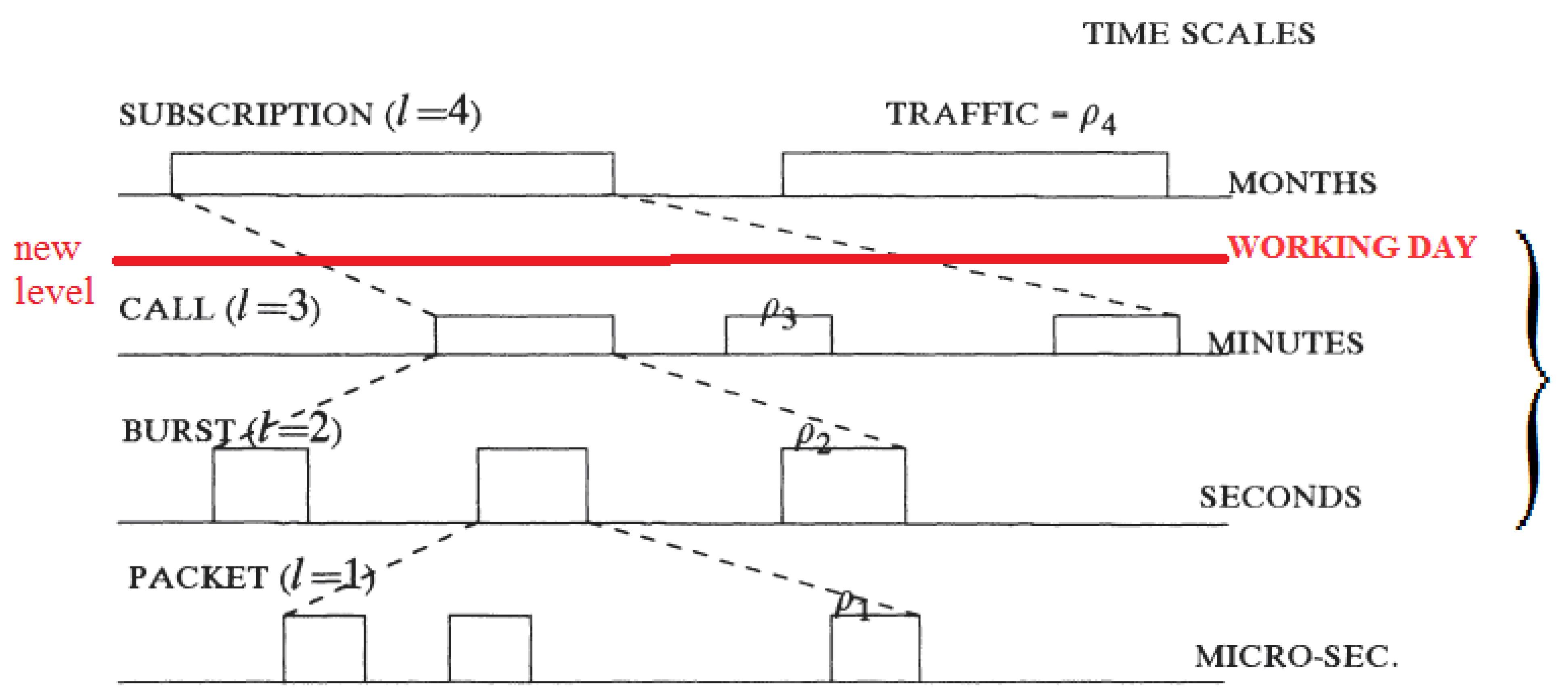
The answer to the latter question may be affirmative. However, before proceeding any further, we need to make the following important remark. In general, the analysis of a process depends on the scale of the consideration. This also applies to data flow analysis. The problem of the data streams’ equivalence may be effectively resolved with some specific choice of scale. In the theory of multi-traffic, the time scales displayed in Figure 2 are distinguished.
The data flows generated by a specific service during a session belong to the scale of “minutes”. In Figure 2, the scale of “seconds” corresponds to “bursts” [10,11,12], and the scale of “microseconds” corresponds to “packets”. We are not concerned with the scale of packets, although simulating communication systems at this scale is very popular nowadays [13,14]. There are toolkits for measuring data flows at both such scales, for example, Tmeter [15]. Thus, the main question is formulated as follows: is it possible to identify a given service on the level of “minutes” and “seconds” or is that the same as “sessions”(“calls” in Figure 2) and “bursts”? This question correlates with the classical metrology [16] approach: one should classify the random processes and determine their numerical characteristics [17] as well as the modern modifications of the classical metrology approaches (see, e.g., [18]).
The data streams that circulate on the Internet are the result of both the operation of Internet services and the activities of the people who use them. The period of human activity at the computer is several hours, and the cycle of this activity is a day, a work shift, exercising a single duty, etc. This initiates the introduction to the scheme in Figure 1 at one more level: a workday. This level accounts for the human factor. There is always a data flow not related directly to a user’s activity: the service data flow. However, this flow is a small part of the total, and, thus, we shall neglect it in this paper.
A user sends no data directly to the Internet, but only starts services or programs creating and/or transferring data to the network. The immediate sources of data are the services initiated by the user.
The Internet is based on data packets technology [13,14,19], and an analysis of the data flow on the Internet theoretically can be based on the study of packets and the protocols of Internet services, for both local and global networks. Unfortunately, keeping track of all possible interactions of these protocols, both among themselves and with the users and a per-packet study of the data flows, are so complex and subject to so many random influences that the analysis of data flow at the microscale (at the scale of data packets) becomes extremely complicated. It is why we do not use the level “microseconds” in Figure 1. In this context, the macroscopic approach is justified: we consider the overall data flow over certain time intervals, for example, seconds, and analyze data flows during the session.
Even on a single computer, multiple services may be run. This raises the question of the interaction of multiple data flows. The latter problem may also be solved by macroscopic analysis.
The aim of this paper is to examine the data flows generated by typical Internet services and the interaction of these flows “at the source”: at a single computer and on the local network.
The basic tool used in this investigation is a series of reliable and reproducible experiments together with the standard statistical methods.
In this paper, the authors present experimental data concerning the output data flows.

2. Data Flow Generated by Popular Internet Services

The main characteristics of data flows are intervals between the events (measured in seconds) and the rate of data exchange (or the data rate, measured in bytes or Kbytes/s.). Hereafter, K means Kbytes/s.
Figure 1 displays a typical fragment of traffic from a single computer when various Internet services are used. The traffic has a strongly inhomogeneous structure: one can distinguish continuous (marked in gray) and discrete fragments of traffic (marked in white or black). The discrete fragments also have various shapes. In Figure 1, one can see fragments that may be identified as independent events (marked in gray or black) and fragments that may be identified as quasiperiodic (marked in white).
We discuss the data flows generated by several widely used Internet services and network applications (information about other Internet services and network applications may be found in [19]).

3. E-Mail Client

The proposed approach is universal and can be applied to arbitrary “sources” of the data stream. It is critically important whether the “source” creates a data flow possessing specific, exactly identified characteristics. In this section, we present our idea in detail, using the example of e-mail. In the next sections, we discuss other Internet services briefly.
We use the following definitions [20]. We call the data stream generated by a specific Internet service in one session the elementary (primitive) data flow from the service. We call the data stream, which is the result of a specific Internet user, the elementary (primitive) data flow from the user.

3.1. Elementary Data Flow from an E-Mail Service

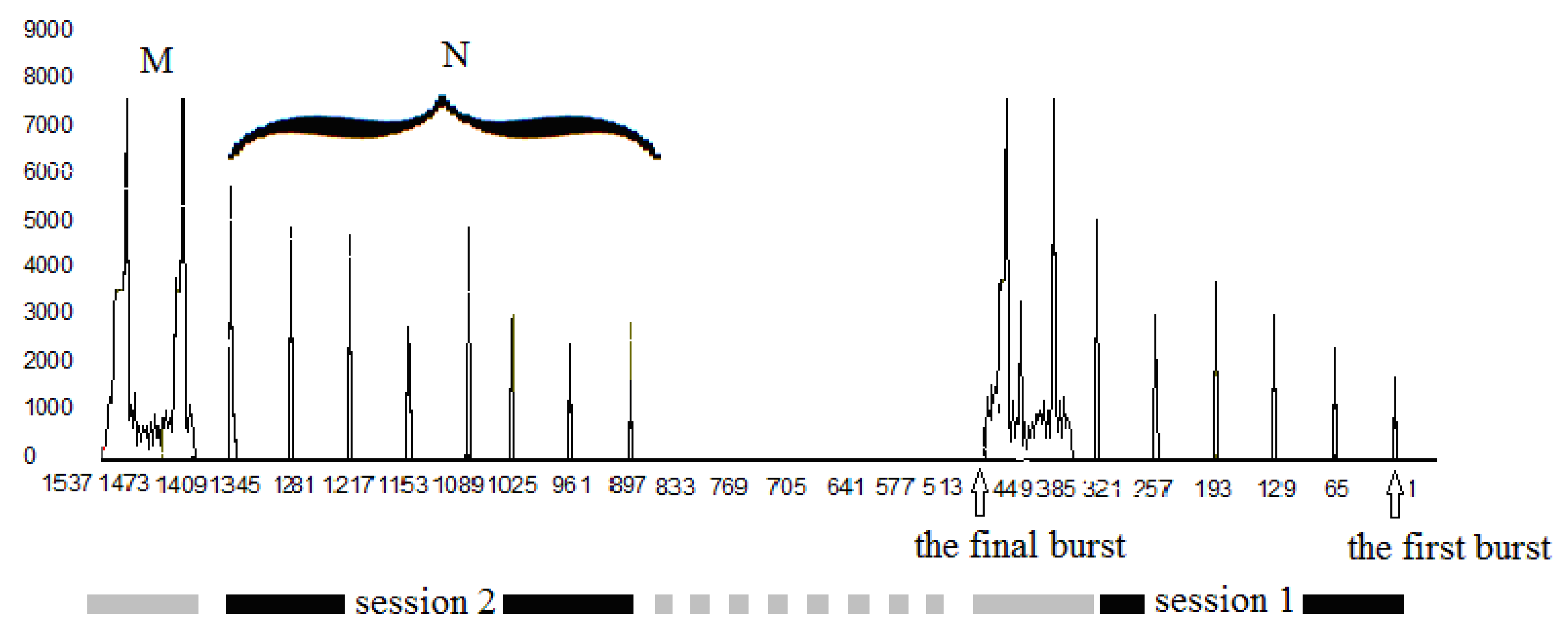
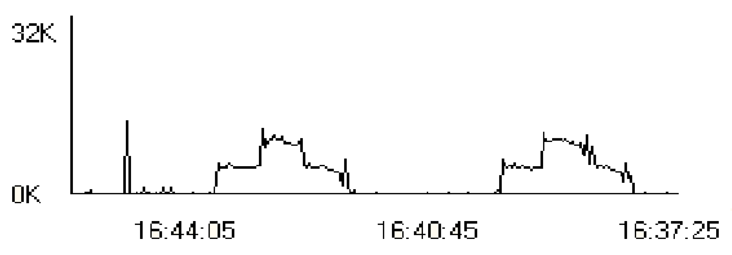
Figure 3 shows the output data rate corresponding to a single e-mail service. The fragments of traffic, marked at the bottom of the figure in black, correspond to the writing of two e-mails (“Session 1” and “Session 2”). The fragments of traffic marked in gray correspond to transmitting e-mails. The fragments of traffic, shown with gray dotted lines, correspond to no user activity. The traffic in this period is determined by the interaction of the user computer with the network.
The numerical characteristics of the traffic are presented in Table 1.
The traffic of one single email session (“CALL” in Figure 1) has a typical form, see Figure 3. It consists of two types of the fragments, marked by us as M and N. First, there are spike-like bursts N that are produced, while the session ends with the ‘final burst” M. The “final bursts” for different email sessions coincide with the first-order approximation.
The fragments of shape N are given by random variables and require statistical analysis. Keeping in mind that our purpose is the modeling of data flows, we have proposed several hypotheses about the possible distributions. Our first hypothesis (Hypothesis 1) is the following: N-bursts come at independent time intervals. Our second hypothesis (Hypothesis 2) is the following: N-bursts have independent amplitudes. By using the Kolmogorov–Smirnov test, we made sure that Hypothesis 1 is true. However, Hypothesis 2 fails. In Figure 3, one can observe that the amplitudes of N-bursts are likely to increase over time. The timeline in Figure 3 is oriented leftwards, which is a particular feature of Tmeter [15]. Our third hypothesis (Hypothesis 3) is the following: the amplitudes have independent increments over the sequence of N-bursts. It turns out that Hypothesis 3 is true.
Thus, we can suggest the following identification for the output data flow of an email application:
-
M-burst that is not random flow;
-
N-bursts that are random flow, which can be identified by the distribution of time intervals between the bursts, the first N-burst amplitude, and the distribution of amplitude increments over the sequence of N-bursts.
The statistical analysis of about 200 e-mails (from 3 to 10 bursts in every e-mail) leads to the conclusion that:
-
the rate increments are normally distributed with the mean of 500 bytes/s and standard deviation of 600 bytes/s;
-
the initial speeds are distributed according to the normal law with a mean of 2500 bytes/s and standard deviation of 700 bytes/s.
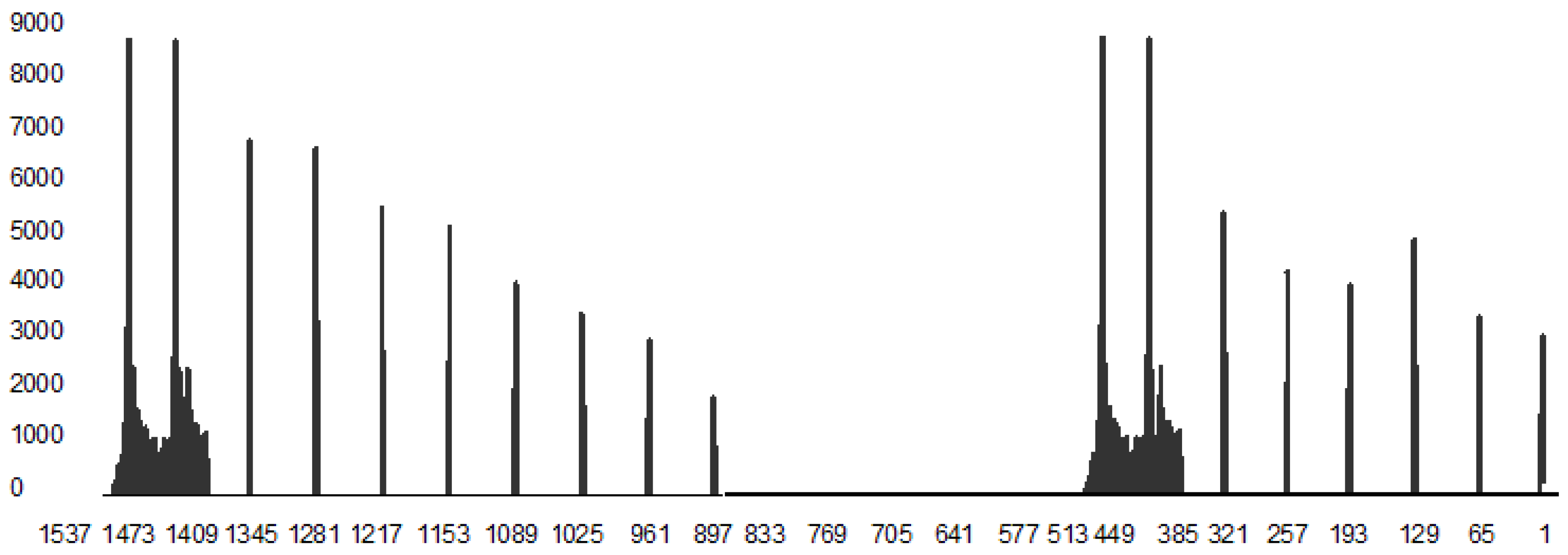
We suggest entering “the passport data” of the elementary data flow from an Internet service. The proposed passport data will be useful if one can reproduce the data stream (traffic) from an Internet service based on its passport data. We have computed “the passport data” for an e-mail service. Now, we try to numerically reproduce the traffic from the e-mail service sessions. The numerically reproduced traffic is shown in Figure 4. The agreement between the experimentally measured traffic in Figure 3 and the numerically reproduced traffic in Figure 4 is good. The numerically reproduced traffic is shown in Figure 4. The agreement between the experimentally measured traffic in Figure 3 and the numerically reproduced traffic in Figure 4 is good.

3.2. User Activity When Using E-Mail

The total traffic depends on the elementary data stream from every e-mail service and user activity. The study of the user activity is the subject of study of physiology, social science, and similar sciences. As we see, the computation of the traffic is an interdisciplinary problem that should be based on the methods of both technical and socioeconomic sciences. Keeping in mind the methodological nature of this paper, we collected data on the typing of small e-mails during correspondence in student groups.The characterictics of the user activity are the time interval between typing each e-mail and the time of typing an e-mail. The corresponding numerical values are presented in Table 2.

4. Organization of Experimental Numerical Simulation

The data flow from one service during one session is called an elementary service flow. In this section, this is the data flow from an e-mail service when one is typing and sending one e-mail. If one knows the passport data of the elementary stream and the users’ activity, one can compute the data stream from an arbitrary number of users.

4.1. Organization of the Experiment

Our computer program is written in the C language and includes:
-
A procedure for modeling an elementary data stream e-mail;
-
A procedure for modeling user activity when using e-mail;
-
A procedure for summing elementary streams;
-
Auxiliary statistical procedures.

4.2. Numerical Experiment Results

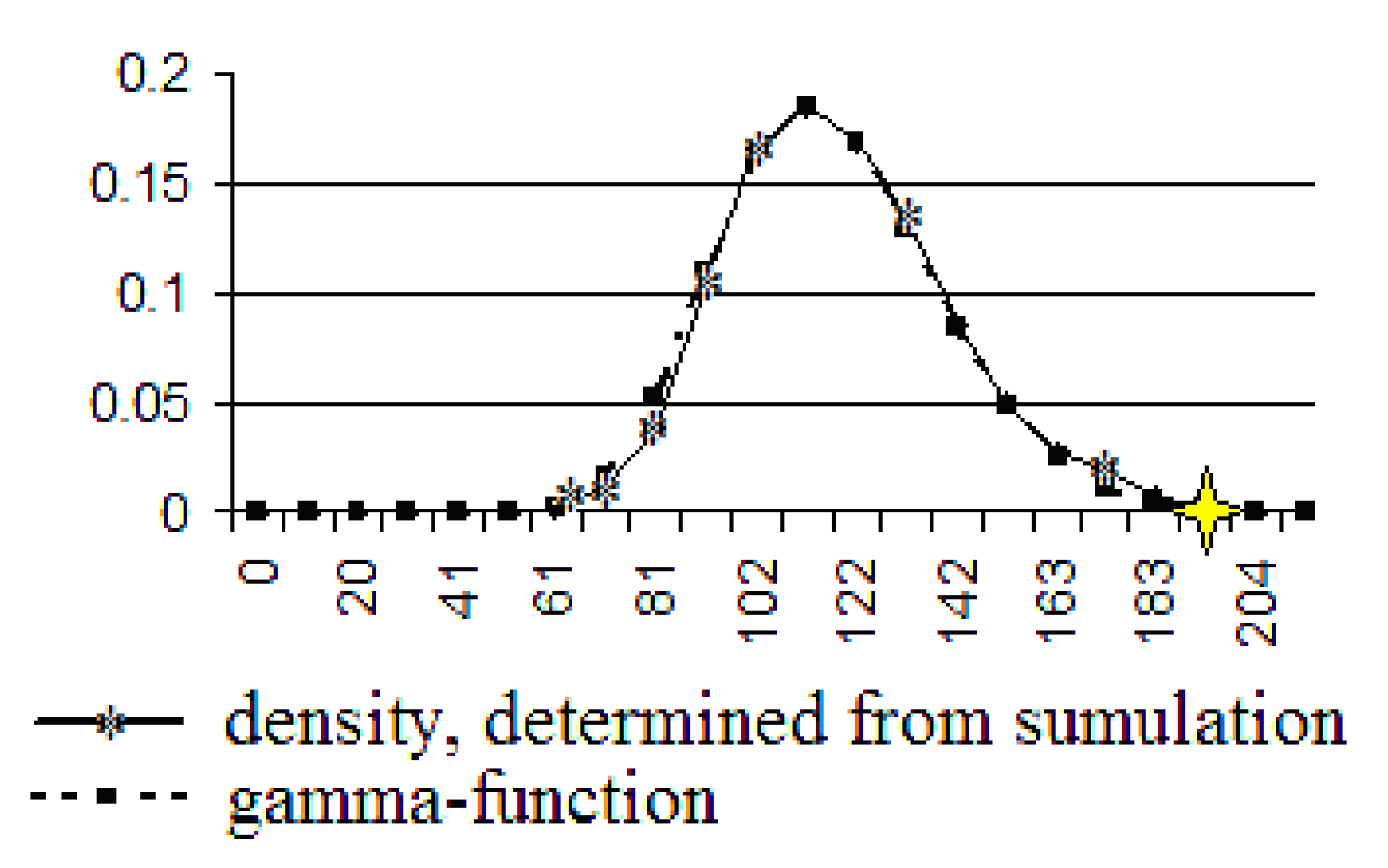
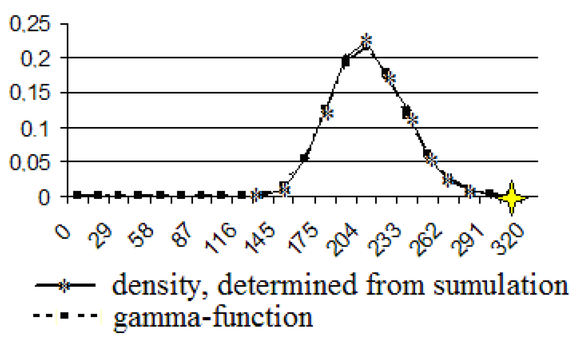
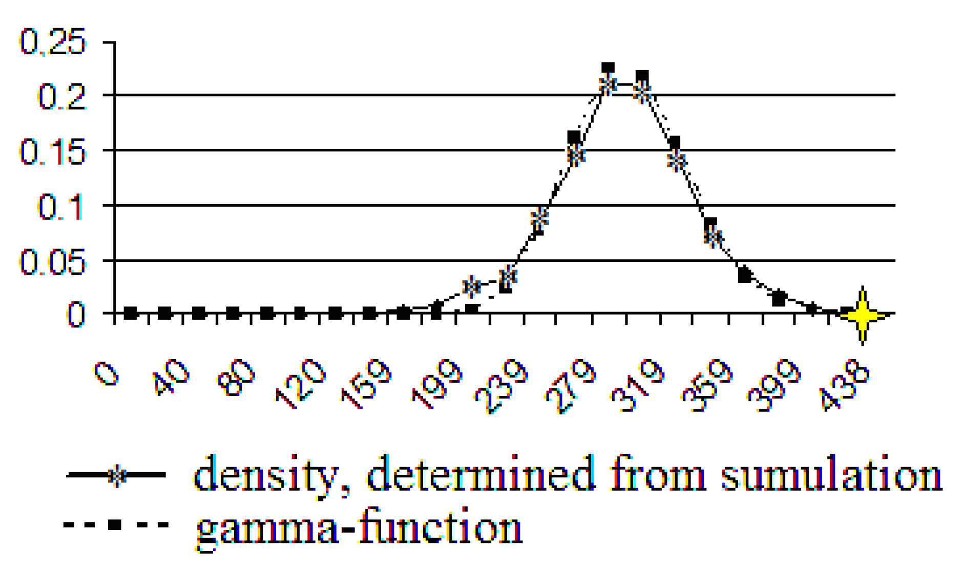
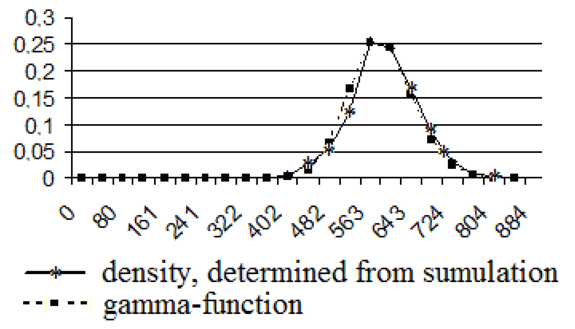
Numerical simulation of the data flow generated by an e-mail service was carried out for number of users from 2 to 2000. In the numerical experiment, the time of continuous work of users in the specified mode (Table 1) is taken as equal to 4 h (half of the workday). The number of users in the numerical experiment varies from 2 to 2000. The actual maximum number of users should be about 1000, because the number of workstations (end-user computers) connected to the Ethernet network is 1024 [21]. Below are the results of the statistical processing of the experimental data. One clearly sees several stages of the transformations of the graph of the density distribution of the data transfer rate. Figure 3, Figure 4, Figure 5, Figure 6 and Figure 7 present graphs of the distribution density of the data transfer rate for 1 to 10 users. The abscissa axis shows the total data transfer rates in K, the ordinate axis shows their probabilities.
Stage 1. Bimodal data rate distribution density is shown in Figure 5. The left peak of the graph in Fig.5 corresponds to cases of an empty (not busy) channel (traffic = 0).
Stage 2. At 20 users, the channel is not empty at any time. As a result, the peak corresponding to the empty channel disappears. The traffic corresponding to stages 1 and 2 is shown in Figure 6a,b, respectively. In the Figure 6, the abscissa axis indicates the time in seconds, while the ordinate axis indicates the transmission rate K/s. Figure 6a,b display three successive time fragments, one under the other, each ½ h long.
Stage 3. The most typical stage, because the number of users of networks usually ranges from several tens to several hundreds. Examination of the traffic in this case, the type of the corresponding data rate distribution and its parameters, is the main content of this work.
Stage 4. When the number of users is more than 1000, the plot of the distribution density of the data transfer rate begins to demonstrate a similarity with the plot of the normal distribution. However, this converges to the normal law very slowly. In reality, the number of users of local networks does not reach the threshold when the normal law is applicable. This happens since the maximum number of stations connected to the Ethernet network is 1024. As shown below, for the number of users in the range of 10–1000, a good approximation of the distribution density of the data transfer rate is the gamma distribution with parameters that depend on the number of users.

5. Construction of the Data Rate Distribution by Using the Computer Simulation

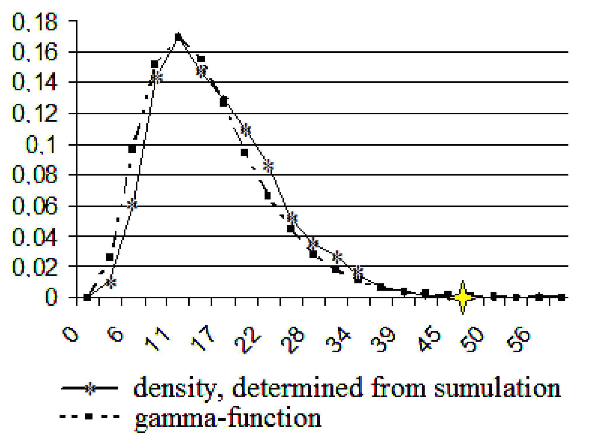
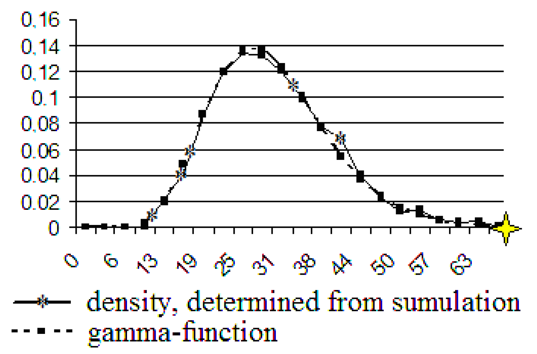
Figure 7, Figure 8, Figure 9, Figure 10, Figure 11, Figure 12, Figure 13, Figure 14 and Figure 15 display the distribution function for the number of users in the range of 20 to 2000.
To propose a hypothesis about the type of distribution, skewness and excess kurtosis (kurtosis in the tables below) were calculated. The results are presented in Table 3 and Table 4.
It follows from Table 3 and Table 4 that the distribution should be selected among the asymmetric distributions. The distributions determined from the simulation have a characteristic form similar to the graphs of the gamma distribution. The gamma distribution density function is given by the following formula.
f ( x ; α , β ) = 1 β α Γ ( α ) x α 1 e x β ,   x 0 ,
where α and β are the parameters [21].
The numerical values of α and β were carried out by the least squares method (the mean square deviation of the empirical distribution functions from the function f ( x ; α , β ) (1) was minimized). The computed parameters are presented in Table 5.
The graphs of the function f ( x ; α , β ) (1) for the parameters indicated in Table 5 and the graphs of the density, determined by using the computer simulation, are shown in Figure 7, Figure 8, Figure 9, Figure 10, Figure 11, Figure 12, Figure 13, Figure 14 and Figure 15. The abscissa axis shows the data rates in K/s, while the ordinate axis shows their probabilities.
An application. In Figure 15, the graphs, for the first time, become similar to the normal distribution, but 2000 users are impossible on a local network. As a result, we conclude that the data rate initiated by e-mail users is described by the gamma distribution.
An application. The results of the statistical analysis presented above have numerical applications. For example, these results provide us with the information about the maximal data stream the function of the user number. This information is useful to estimate the necessary local network capacity and the data stream from this local network to the global network. The maximum data rate is marked in Figure 7, Figure 8, Figure 9, Figure 10, Figure 11, Figure 12, Figure 13 and Figure 14 by an asterisk, and the corresponding numerical values of the rate (in K) are presented in Table 6.

6. Justification of the Constructed Density of the Data Flow Rate

Visually, there is a good match between the plots of the distribution functions determined from the computer simulations and the plots of the distribution density functions of the gamma distribution in Figure 7, Figure 8, Figure 9, Figure 10, Figure 11, Figure 12, Figure 13, Figure 14 and Figure 15. We present the statistical justification for this conclusion. We propose the following hypothesis: the data rate determined from our computer simulation has a gamma distribution with the parameters indicated in Table 5.
To verify/reject this hypothesis, we use the Kolmogorov–Smirnov test [22], which consists of the following: as a measure of the discrepancy between the theoretical and statistical distributions, the maximum value of the modulus of the difference between the statistical distribution function F * ( x ) and the corresponding theoretical distribution function F ( x ) is considered:
D = max | F * ( x ) F ( x ) |
The critical value of the Kolmogorov–Smirnov test is calculated by the formula λ = D n , where n is the number of relative empirical frequencies. The probability P ( λ ) is determined from the table from [22] ( P ( λ ) is the probability that, due to purely random reasons, the maximum discrepancy between F * ( x ) and F ( x ) will be no less than the one that is actually observed [22]). If P ( λ ) is close to 1, then the hypothesis of the gamma distribution of the computer-simulated data transfer rate is accepted. At a value close to zero, this hypothesis is rejected, see [22] for details.
The calculated values λ and P ( λ ) are presented in Table 7.
Since the probabilities P ( λ ) from Table 7 are close to 1, then we accept the hypothesis of the gamma distribution of the simulated frequencies.

7. Other Internet Services: Internet Browsing, File Transfer, etc.

The detailed exposition of the proposed approach was presented for an Internet e-mail service. Briefly, we discuss some other Internet services.

7.1. Internet Browsing

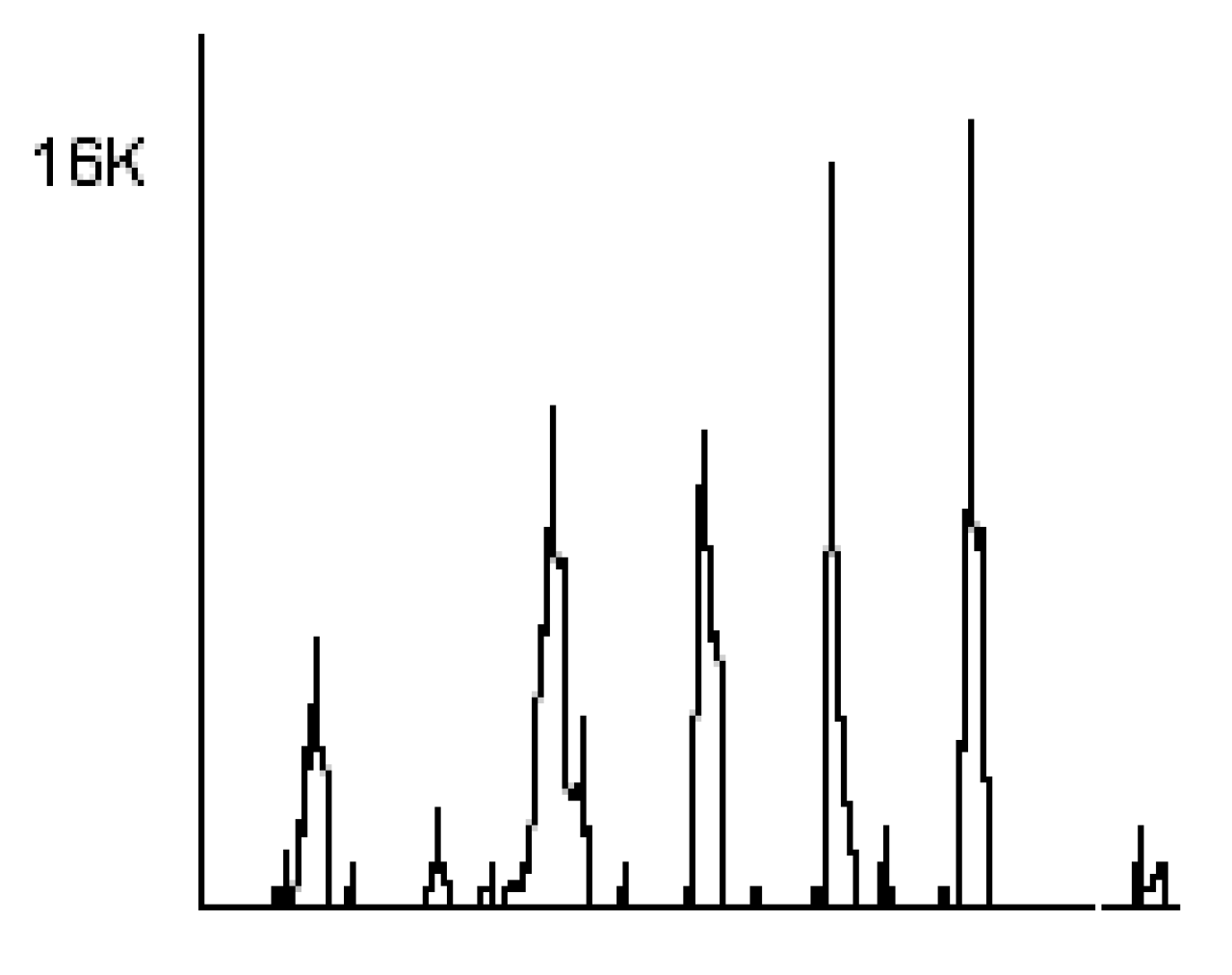
Figure 16 shows the output data rate corresponding to browsing webpages. Here, the events are discrete in nature. The time between the events is determined by the user’s activity.
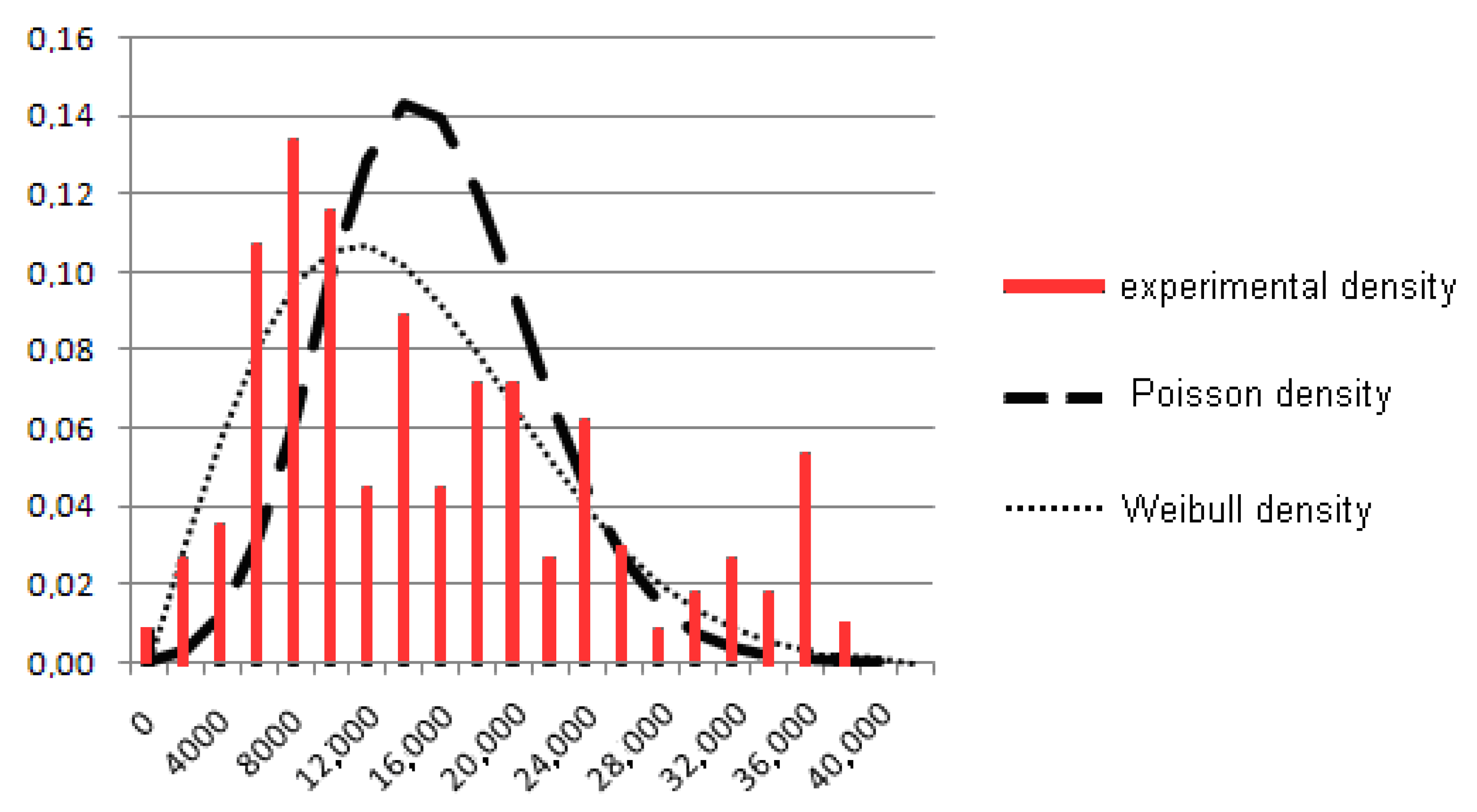
We present the results of the statistical analysis of the data rates. There were held views of webpages in the search mode—users searched for thematic information. Each user visits no more than one site per 10 s. The experimental data rates were in the range of from 2000 to 40,000 bytes/s. The expected value of the data rate is 15,589.
Figure 17 displays the experimental distribution function of the data rate. The graph of the Poisson function with the same expected value is displayed. We observe that the experimental distribution function is significantly different than the Poisson distribution. A better approximation for the experimental distribution function is given by the Weibull distribution function with parameters α = 2 and β = 8. For the data presented in Figure 17, the sample variance is equal to 9395.617, the asymmetry coefficient is equal to 0.761881, and the kurtosis is equal to 0.32556. The experimental distribution is strongly asymmetric.
The asymmetry of the experimental distribution function and a slow decay in the right part of the chart are clearly seen in Figure 17. Thus, the shape of the distributions with “heavy tails” occurs at the level of an elementary data stream, which is a stream from a single computer.

7.2. File Transfer over the Internet

Figure 18 shows the data rates corresponding to the transfer of files to a remote computer. The sizes of files are in the range 100 to 2000 K, and increase with a step of 100 K. The three series of experiments are displayed; every series is marked in gray.
An application. The average data rate depends on the file size. The result of the statistical processing of the data presented in Figure 18 is shown in Figure 19 (the file size being displayed on the horizontal axis and the transmission rate on the vertical axis).

8. Superposition of Data Streams Generated by Internet Services

The problem of the superposition of data streams on computer networks is fundamental for the simulation and computation of the data streams on the computer networks. This problem is a non-trivial one. On one hand, the assumption that the data streams are accurately summed up on the “nodes” of the network is widely used. On the other hand, various methods of data compression [23] are widely used. Thus, the problem of the data flows interaction should be considered in relation to a particular data-transmission technology. We investigate this issue, as applied to the typical services and typical local Internet networks.

8.1. Superposition of Data Streams on a Single Computer

The problem of the interaction of data flows already arises for a single computer, while working with several Internet services.
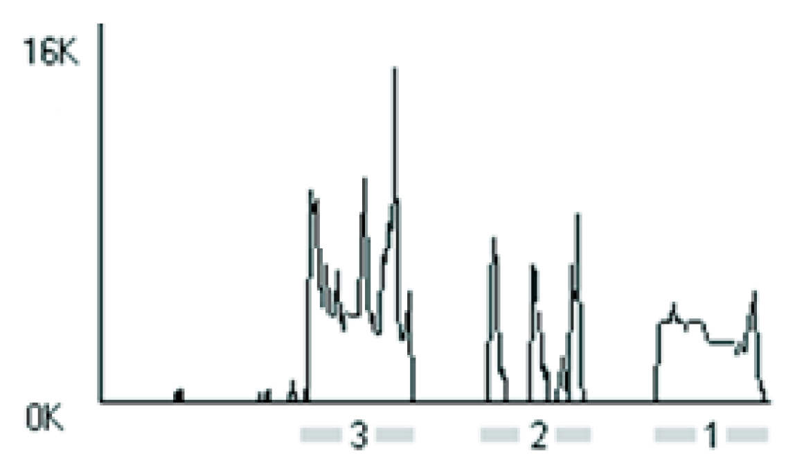
Figure 20 shows the traffic when a user runs several Internet programs simultaneously, in this case the audio communication program Skype and a web browser. Fragment 1 corresponds to using Skype solely, Fragment 2 corresponds to browsing an Internet page without the use of Skype, and Fragment 3 corresponds to browsing an Internet page during a Skype talk.
As can be seen, the transfer rates are summed (the transmission rate for process 3, with a slight error, is the sum of the rates for processes 1 and 2). This fact has been verified for numerous data streams. It holds valid until the channel capacity is not exceeded.

8.2. Superposition of Data Streams from Different Computers

Figure 21 shows a typical local network. Data flows are initiated by users in different time moments. The output streams arrive at a server computer, which creates an output stream from the server to the Internet.
We present the results of our experimental measurements of the output data rates on user computers on a network and the server, by using Skype as a working example.
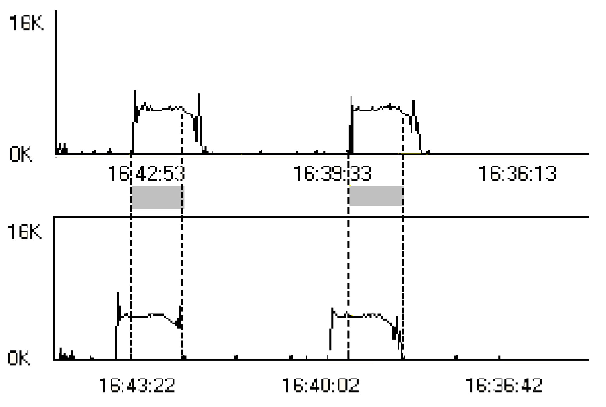
Figure 22 shows the output streams from two computers during independent Skype sessions. Figure 23 shows the output stream from the commutator during the same period of time. The gray bars mark the superposition of the streams.
To calculate the sum of the data rates presented in Figure 22 and compare it with the data rate of the output stream on the commutator (displayed in Figure 23), we carried out a digitization of the graphs in Figure 22 and Figure 23. Three arrays were made: the data rate X 1 [ i ] corresponding to the first computer, the data rate X2[i] corresponding to the second computer, and the data rate X0[i] corresponding to the server (a commutator device that was installed on the server). One can easily perform arithmetic operations with the elements of these arrays.
The graph of the sum X1[i] + X2[i], the graph of the experimentally measured output data rate from the server X0[i], and the difference X1[i] + X2[i] − X0[i] are shown in Figure 24.

8.3. Superposition of Three Data Streams

Figure 25 presents the output streams of three computers during Skype sessions. These sessions overlap in time (the overlapping periods of sessions are marked in gray).
Figure 26 shows the output stream on the commutator (server) for the same period of time.
To calculate the sum of the data rates presented in Figure 25 and to compare it with the data rate presented in Figure 26, a digitization of these graphs was carried out. There were built four numeric arrays: output data rate X1[i] from the first computer, output data rate X2[i] from the second computer, output data rate X3[i] from the third computer, and output data rate X0[i] from the server.
The graph of the sum of X1[i] + X2[i] + X3[i], the graph of the experimentally measured output stream on the server X0[i], and the difference of X1[i] + X2[i] + X3[i] − X0[i] are shown in Figure 27. The average value of the relative deviation (X1[i] + X2[i] + X3[i] − X0[i])/X0[i] does not exceed 5%.

9. Conclusions

The information about the individual characteristics of the data streams generated “at the source”, the superposition of these streams, and a specific user’s activity allow for computing the total data streams on the network.
The authors suggest analyzing the characteristics of traffic generated by Internet services and to develop data rate “portraits” (or “passports”) of these services. The development of the “portraits” (or “passports”) of services assumes a statistical investigation of these services. Examples of such analysis are presented for the most common Internet services. A detailed analysis is presented for an e-mail service.
The authors experimentally investigated the superposition of data streams on a local network and found that the data rates are additive, with the relative error less than 5%. The authors found that the additive rule is not satisfied exactly.
These results may be used for the development of models of the data streams, based on the “passport data” for the Internet services and the statistical information about users’ activity. The models may be used to compute the total data flow on the local network, depending on the users’ activity: the types of services, the number of users, the users’ activity, etc. (see examples in the subsections titled “An application”).

Author Contributions

Conceptualization, methodology, experiments, formal analysis, software, validation, investigation, writing—original draft preparation, N.A.F.; supervision, A.G.K.; resources, S.I.R. All authors have read and agreed to the published version of the manuscript.

Funding

This research received no external funding.

Data Availability Statement

Not applicable.

Acknowledgments

N.A.F. thanks V.I.Meikshan (Siberian State University of Telecommunications and Informatics) for the fruitful discussions.

Conflicts of Interest

The authors declare no conflict of interest.

References

  1. Liu, D.; Xu, X.; Liu, M.; Liu, Y. Dynamic traffic classification algorithm and simulation of energy Internet of things based on machine learning. Neural Comput. Appl. 2021, 33, 3967–3976. [Google Scholar] [CrossRef]
  2. WłodarskI, P. Impact of Long-Range Dependent Traffic in IoT Local Wireless Networks on Backhaul Link Performance. In International Conference on Computational Science—ICCS 2020; Springer: Cham, Switzerland; Berlin/Heidelberg, Germany, 2020; pp. 423–435. [Google Scholar]
  3. Data Volume of Global Consumer Internet Traffic from 2017 to 2022, by Subsegment. Available online: https://www.statista.com/statistics/267194/forecast-of-internet-traffic-by-subsegment/ (accessed on 1 June 2022).
  4. Erlang, A.K. Probability and telephone calls. Nyt Tidsskr. Mat. B 1909, 20, 33–39. [Google Scholar]
  5. Erlang, A.K. Losning af nogle problemer fra sandsynlighedsregningen af betydning for de automatiske telefoncentraler. Elektroteknikeren 1917, 13, 5–13. [Google Scholar]
  6. Pollaczek, F. Über eine Aufgabe der Wahrscheinlichkeitstheorie. Math. Z. 1930, 32, 64–100. [Google Scholar] [CrossRef]
  7. Kendall, D.G. Stochastic processes occurring in the theory of queues and their analysis by the method of the imbedded Markov chain. Ann. Math. Stat. 1953, 24, 338–354. [Google Scholar] [CrossRef]
  8. Roberts, J.; Mecca, U.; Virago, J. (Eds.) Broadband Network Teletraffic: Performance Evaluation and Design of Broadband Multiservice Networks, Final Report of Action COST 242; Springer: Berlin/Heidelberg, Germany, 1996. [Google Scholar]
  9. Akimaru, H.; Kawashima, K. Teletraffic: Theory and Applications (Telecommunication Networks and Computer Systems), 2nd ed.; Springer: New York, NY, USA, 2012. [Google Scholar]
  10. Hui, J.N. Switching and Traffic Theory for Integrated Broadband Networks; Springer: New York, NY, USA, 2012; Volume 91. [Google Scholar]
  11. Willinger, W.; Leland, W.; Taqqu, M.; Wilson, D. On the Self-Similar Nature of Ethernet Traffic. IEEE/ACM Trans. Netw. 1994, 2, 1–15. [Google Scholar] [CrossRef] [Green Version]
  12. Schmid, S.; Wattenhofer, R. Dynamic Internet Congestion with Bursts. In High Performance Computing—HiPC 2006; Robert, Y., Parashar, M., Badrinath, R., Prasanna, V.K., Eds.; Springer: Berlin/Heidelberg, Germany, 2006; Volume 4297. [Google Scholar]
  13. Jeruchim, M.C.; Balaban, P.; Shanmugan, K.S. Simulation of Communication Systems: Methodology and Techniques; Springer: New York, NY, USA, 2000. [Google Scholar]
  14. Rorabaugh, C.B. Simulating Wireless Communication Systems; Prentice Hall: Hoboken, NJ, USA, 2004. [Google Scholar]
  15. TMeter Freeware Edition. Available online: http://tmeter.ru/ (accessed on 1 June 2022).
  16. Mekid, S. Metrology and Instrumentation: Practical Applications for Engineering and Manufacturing; Wiley-ASME Press: Hoboken, NJ, USA, 2022. [Google Scholar]
  17. Crowder, S.; Delker, C.; Forrest, E.; Martin, N. Introduction to Statistics in Metrology; Springer: Cham, Switzerland; Berlin/Heidelberg, Germany, 2020. [Google Scholar]
  18. Loh, T.H. (Ed.) Metrology for 5G and Emerging Wireless Technologies (Telecommunications); The Institution of Engineering and Technology: London, UK, 2022. [Google Scholar]
  19. Kurose, J.F.; Ross, K.W. Computer Networking: A Top—Down Approach, 6th ed.; Pearson: Boston, MA, USA, 2012. [Google Scholar]
  20. Filimonova, N.A. Model of elementary stream in Internet. In Distributed Informational and Computational Resources, 26–30 November 2012; Siberian Branch of Russian Academy of Sciences: Novosibirsk, Russia, 2012. [Google Scholar]
  21. Chowdhury, D.D. High Speed LAN Technology Handbook; Springer: Berlin/Heidelberg, Germany, 2000. [Google Scholar]
  22. Olofsson, P.; Andersson, M. Probability, Statistics, and Stochastic Processes, 2nd ed.; Wiley: New York, NY, USA, 2012. [Google Scholar]
  23. Dumas, J.G.; Roch, J.L. Foundations of Coding: Compression, Encryption, Error Correction; Wiley: New York, NY, USA, 2015. [Google Scholar]
Figure 1. Typical fragment of traffic.
Computers 11 00138 g001
Figure 2. Time scales in multi-traffic theory.
Computers 11 00138 g002
Figure 3. The output data rate corresponding to typing and sending two e-mails. Experimental data.
Computers 11 00138 g003
Figure 4. Simulating the data flow of two e-mail sessions by a computer program.
Computers 11 00138 g004
Figure 5. The data rate density computed from computer simulation: 1, 5, and 10 users. E-mailing.
Computers 11 00138 g005
Figure 6. (a) Traffic for 5 users, computer simulation, where traffic is zero about 50% of the time. (b) Traffic for 5 users, computer simulation, where traffic is not zero most of the time.
Computers 11 00138 g006
Figure 7. The gamma function and the density, determined by using computer simulation. The number of users is 20.
Computers 11 00138 g007
Figure 8. The gamma function and the density, determined by using computer simulation. The number of users is 50.
Computers 11 00138 g008
Figure 9. The gamma function and the density, determined by using computer simulation. The number of users is 100.
Computers 11 00138 g009
Figure 10. The gamma function and the density, determined by using computer simulation. The number of users is 200.
Computers 11 00138 g010
Figure 11. The gamma function and the density, determined by using computer simulation. The number of users is 500.
Computers 11 00138 g011
Figure 12. The gamma function and the density, determined by using computer simulation. The number of users is 700.
Computers 11 00138 g012
Figure 13. The gamma function and the density, determined by using computer simulation. The number of users is 900.
Computers 11 00138 g013
Figure 14. The gamma function and the density, determined by using computer simulation. The number of users is 1000.
Computers 11 00138 g014
Figure 15. The gamma function and the density, determined by using computer simulation. The number of users is 2000.
Computers 11 00138 g015
Figure 16. The output data rate corresponding to browsing five webpages.
Computers 11 00138 g016
Figure 17. Experimental density function for the data rate and the Poisson and Weibull density functions.
Computers 11 00138 g017
Figure 18. Experimental data rates corresponding to file transfer.
Computers 11 00138 g018
Figure 19. The average data transfer rate as a function of file size.
Computers 11 00138 g019
Figure 20. Summation of the data rates on a single computer.
Computers 11 00138 g020
Figure 21. Superposition of data streams from different computers on a server.
Computers 11 00138 g021
Figure 22. Output streams (Skype sessions) from two computers.
Computers 11 00138 g022
Figure 23. The output stream from commutator (server).
Computers 11 00138 g023
Figure 24. Comparison of the data streams.
Computers 11 00138 g024
Figure 25. Output streams from three computers (data rates).
Computers 11 00138 g025
Figure 26. Output stream from a server (data rate).
Computers 11 00138 g026
Figure 27. Comparison of data streams.
Computers 11 00138 g027
Table 1. Characteristics of N-bursts.
Parameter NameParameter Value
Rate in the first burst 1.2–2.9 K/s
Time interval between the bursts 64–68 s
Burst duration0–2 s
Table 2. Characteristics of the users’ activity.
Parameter NameParameter Value
Time interval between typing each e-mail10 min
Time of typing an e-mail6–7 min
Table 3. Skewness and kurtosis of empirical distribution functions.
Number of Users203050100200300400
skewness1.6691.3241.0470.7271.1500.9901.245
kurtosis1.6220.8180.4111.0810.0030.5590.054
Table 4. Skewness and kurtosis of empirical distribution functions.
Number of Users50060070080090010002000
skewness 1.2451.5681.5021.5641.7221.5641.850
kurtosis 0.0541.2760.9181.0992.0871.2342.396
Table 5. Parameters α and β , depending on the number of users.
Number of Users20305010020030040050060070080090010002000
α 33.849.9192525.427.24956.960647190
β 1.82.33.7333.64.64.33.63.644.24.16.5
Table 6. The maximum data rate, depending on the number of users.
Number of Users20501002005007009001000
max data rate, K255070110200320410440
Table 7. Critical value of the Kolmogorov–Smirnov test λ and values of distribution probabilities P ( λ ) .
Number of Users2030501002003004005006007008009001000
λ 0.7410.5670.6650.2770.6340.3750.5530.5250.5180.5350.5310.4970.423
P ( λ ) 0.7110.9640.86410.86410.9640.9640.9640.9640.9640.9970.997
Publisher’s Note: MDPI stays neutral with regard to jurisdictional claims in published maps and institutional affiliations.