Abstract
Short-term electric power load forecasting is a critical and essential task for utilities in the electric power industry for proper energy trading, which enables the independent system operator to operate the network without any technical and economical issues. From an electric power distribution system point of view, accurate load forecasting is essential for proper planning and operation. In order to build most robust machine learning model to forecast the load with a good accuracy irrespective of weather condition and type of day, features such as the season, temperature, humidity and day-status are incorporated into the data. In this paper, a machine learning model, namely a regression tree, is used to forecast the active power load an hour and one day ahead. Real-time active power load data to train and test the machine learning models are collected from a 33/11 kV substation located in Telangana State, India. Based on the simulation results, it is observed that the regression tree model is able to forecast the load with less error.
1. Introduction
An electric power distribution substation takes the power from one or more transmission or subtransmission lines and delivers this power to residential, commercial, and industrial customers through multiple feeders. Short-term load forecasting at the distribution level estimates the active power load on a substation in a time horizon ranging from 30 min to 1 week [1]. The load forecasting of a distribution system gives advance alarms to the operator about the overloading of feeders and substations. Load forecasting helps the distribution substation operator to schedule and dispatch the storage batteries to shave the peak load in a smart grid environment [2]. Electrical power load forecasting is classified as very short term, short term, medium term and long term based on the length of the prediction horizon [3,4,5]. Due to deregulated power system structure and more liberalization in energy markets, electric power load forecasting has become more essential [6]. Long-term load forecasting is generally used for planning and investment profitability analysis, determining upcoming sites, or acquiring fuel sources for production plants. Medium-term load forecasting is usually preferred for risk management, balance sheet calculations, and derivatives pricing [7]. An accurate short-term load forecasting will help an electric power distribution utility to optimize the power grid load and strengthen reliability, reduce the electricity consumption cost and emphasize electric energy trading possibilities.
Forecasting the distribution-level load is far more challenging than forecasting the system-level load, such as the Telangana State’s electric power demand, due to the intricate load characteristics, huge number of nodes, and probable switching actions in distribution systems. Since the end-user behaviour has a far greater influence on distribution systems than it does on transmission systems, the load profiles of distribution systems will have more stochastically abrupt departures. Operating an independent distribution system successfully necessitates significantly more precise and high-resolution load forecasting than today’s approach can deliver [8]. Load estimates over a vast region are highly accurate because the aggregated load is steady and consistent. The distribution-level load, on the other hand, may be dominated by a few major clients, such as industrial businesses or schools, and the load pattern may not be as regular as that of a vast region. Furthermore, due to reconfigurations caused by switching activities, the load may be temporarily moved from one feeder to another, causing significant changes in distribution-level load profiles and affecting the trend at a given time. The main challenge in electric power load forecasting is data loss. Some works are available in the literature to deal with data loss, e.g., by designing a voltage hierarchical controller against communication delay and data loss [9]. The communication delay was treated using delay-tolerant power compensation control (DTPCC) in [10]. PCC uses normal PCC for effective operation when the communication delay is within the maximum tolerable communication delay, or switches to predictive PCC under abnormal communication delay conditions. However, in that paper, the authors collected historical data from the distribution company not through any communication channels.
Four general categories are identified for short-term load forecasting, i.e., similar day, variable selection, hierarchical forecasting, and weather station selection [11]. The similar-day technique identifies the load data as a set of related daily load profiles, whereas the variable selection method assumes that the load data act as a series of variables that are either correlated or independent of one another. The hierarchical technique, on the other hand, treats data as an aggregated load that is extremely variable due to changes in the load at the lower levels of the hierarchy. Finally, weather station selection is a strategy for determining which weather data are best fitted into the load model [12]. Load forecasting is regarded as one of the most critical duties for power system operators in the demand management system (DMS) as shown in Figure 1.
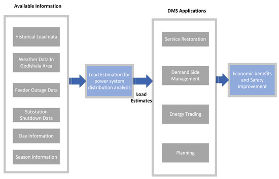
Figure 1.
Main functions of a distribution management system.
Many researchers have been working on short-term load forecasting of distribution systems. An ANN-based methodology was developed in [13] to forecast the load on a 33/11 kV substation near Kakatiya University in Warangal, Telangana State. In that study, the authors used the load from the previous three hours and the load at the same time but in the previous four days as input features. Load forecasting on an electric power distribution system using various regression models was proposed in [14] by considering the load from the previous three hours and the load at the same time but on the previous day as input features. Short-term load forecasting on an electric power distribution system using factor analysis and long short-term memory was proposed in [15] by considering the load from the previous three hours, the load at the same time but in the previous three days, and the load at the same time but in the previous three weeks as input features. Electric power load forecasting at the distribution level using a random forest and gated recurrent unit was proposed in [16], by considering previous three hours load, load at same time but previous three days and load at same time but previous three weeks as input features. Electric power load forecasting at the distribution level using a correlation concept and an ANN was proposed in [17] by considering the load from the previous two hours and the load at the same time but in the previous three days as input features. Similarly, the active power demand on a 33/11 kV electric power distribution system using principal component analysis and a recurrent neural network was proposed in [18], by considering the load from the previous three hours, the load at the same time but in previous three days and the load at the same time but in previous three weeks as input features.
Electric power load forecasting on a medium voltage level based on regression models and ANN was proposed in [19] using time series DSO telemetry data and weather records from the Portuguese Institute of Sea and Atmosphere, and applied to the urban area of Évora, one of Portugal’s first smart cities. A new top-down algorithm based on a similar day-type method to compute an accurate short-term distribution loads forecast, using only SCADA data from transmission grid substations was proposed in [20]. That study was evaluated on the RBTS test system with real power consumption data to demonstrate its accuracy. A convolutional-neural-network-based load forecasting methodology was proposed in [21]. Electric demand forecasting with a jellyfish search extreme learning machine, a Harris hawks extreme learning machine, and a flower pollination extreme learning machine was discussed in [22]. Electric power load forecasting using gated recurrent units with multisource data was discussed in [23]. Short-term load forecasting using a niche immunity lion algorithm and convolutional neural network was studied in [24]. Electricity demand forecasting using a dynamic adaptive entropy-based weighting was discussed in [25]. A demand-side management technique by identifying and mitigating the peak load of a building was studied in [26]. Electric power demand forecasting using a vector autoregressive state-space model was discussed in [27].
Electric power load forecasting using a random forest model was discussed in [28]. In that study, authors considered wind speed, wind direction, humidity, temperature, air pressure, and irradiance as input features. Electric power load forecasting using a group method of data handling and support vector regression was discussed in [29]. The electric power load prediction at the building and district levels for day-ahead energy management using a genetic algorithm (GA) and artificial neural network (ANN) power predictions was discussed in [30]. Short-term electric power load forecasting using feature engineering, Bayesian optimization algorithms with a Bayesian neural network was discussed in [31]. Active power load forecasting using a sparrow search algorithm (ISSA), Cauchy mutation, and opposition-based learning (OBL) and the long short-term memory (LSTM) network was studied in [32]. A new hybrid model was proposed in [33] based on CNN, LSTM, CNN_LSTM, and MLP for electric power load forecasting. All these methodologies provided valuable contributions towards the load forecasting problem, but these studies did not include the weather impact, season and day status in load forecasting.
The main contributions of this paper are as follows:
- A new active power load dataset is developed to work on load forecasting problem by collecting the data from a 33/11 kV distribution substation in Godishala (village), Telangana State, India and available at https://data.mendeley.com/datasets/tj54nv46hj/1, accessed on 1 May 2022.
- A machine learning model, i.e., a regression tree model is used to forecast the load on a 33/11 kV distribution substation in Godishala.
- The active power load on a 33/11 kV substation is forecast one hour ahead based on input features L(T-1), L(T-2), L(T-24), L(T-48), day, season, temperature, and humidity.
- The active power load on a 33/11 kV substation is forecast one day ahead based on input features L(T-24), L(T-48), day, season, temperature, and humidity.
- A web application is developed based on a regression tree model to forecast the load on a 33/11 kV distribution substation in Godishala.
- The impact of weather and days on short-term load forecasting is analysed by incorporating the season and day-status (weekday/weekend) in the data.
- A practical implementation of the system in a prototype web application, where a regression tree model is deployed and execute the forecasts on a daily and hourly basis.
2. Methodology
This section presents the active power load data that are used to train and test the machine learning models. Furthermore, we discuss about the regression tree model that is used for electric power load forecasting on a 33/11 kV distribution substation in Godishala. This substation has four feeders: the first feeder (F1) supplies load to Godishala (town), the second feeder supplies load to Bommakal, the third feeder supplies load to the Godishala (village), and the fourth feeder (F4) supplies load to Raikal. The complete pipeline to develop the web application for short-term load forecasting using a regression model is presented in Figure 2.
2.1. Active Power Load Data Analysis
To train and test the machine learning model, active power load data are required. Hourly data consisting of voltage (V), current (I) and power factor (cos()) from a 33/11 kV distribution substation in Godishala were collected from 1 January 2021 to 31 December 2021. Based on these data, the hourly active power load was calculated using Equation (1) and the sample load data are presented Table 1.

Table 1.
Sample load data for first 5 h on 1 January 2021 at the 33/11 kV substation in Godishala.
2.2. Features Information and Data Preparation
In this paper, the load at a particular time of the day “L(T)” was predicted based on the last two hours of load data, i.e., L(T-1), L(T-2), the load at the same time but in the last two days, i.e., L(T-24), L(T-48), the temperature, the humidity, the season, and the day. Hence, data that were prepared based on collected information from the 33/11 kV substation were rearranged as shown in Table 2. This was the approach used for hour-ahead forecasting, whereas for day-ahead forecasting, the load at a particular time of the day “L(T)” was predicted based on the load at the same time but in the last two days, i.e., L(T-24), L(T-48), the temperature, the humidity, the season, and the day as presented in Table 3. The dataset for hour-ahead forecasting had 8712 samples, 8 input features and 1 output feature. Similarly, the dataset for day-ahead forecasting had 8712 samples, 6 input features and one output feature.
Table 2.
First 6 samples from the dataset which was used to train and test the machine learning models for hour-ahead forecasting.
Table 3.
First 6 samples from the dataset which was used to train and test the machine learning models for day-ahead forecasting.
2.3. Machine Learning Models
In this paper, a regression tree model was used to forecast the load on a 33/11 kV substation one hour ahead and one day ahead. The problem discussed here is a regression problem. Models need to predict the load on the substation based on input features such as L(T-1), L(T-2), L(T-24), L(T-48), day, season, temperature, and humidity in the case of hour-ahead forecasting, and based on input features such as L(T-24), L(T-48), day, season, temperature, and humidity in the case of day-ahead forecasting. The performance of each machine learning model for electric power load forecasting on a 33/11 kV substation was observed in terms of the MSE as shown in Equation (2)
Regression Tree
A regression tree is basically a decision tree model that is used for the task of regression, which can be used to predict continuous valued output. In this paper, a regression tree was used to forecast the load. For a regression problem, a tree is constructed by splitting the input features such that the mean squared error shown in Equation (3) is minimum. A step-by-step procedure to construct the regression tree with sample data is explained in Appendix B, as mentioned in Algorithm 1. The performance of the regression tree model on short-term load forecasting problem for Godishala substation was measured in terms of error metrics such as the MSE [34], RMSE [35,36,37], and MAE [38]. A decision tree can also used for classification problems [39,40,41].
| Algorithm 1 Regression tree model formulation |
|
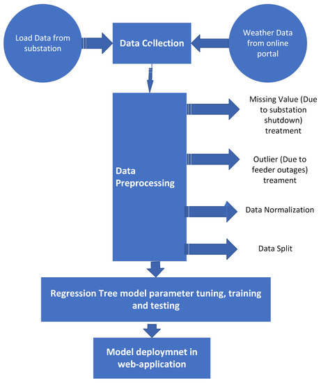
Figure 2.
Workflow to develop web application.
3. Result Analysis
All the machine learning models were developed based on the data available in [42] using Google Colab. this section presents the data analysis, training and testing performance of machine learning models, and the web application developed to predict the load. Out of 8712 samples, 95% of samples were used for training and the remaining 5% of samples were used for testing. The data processing techniques for observing the data distribution and outliers and for data normalization were used before using these data to train and test the regression model. A stochastic gradient descent optimizer was used to train the regression models.
3.1. Regression Tree Model
The performance of the regression tree model that was developed to forecast the load L(T) based on features L(T-1), L(T-2), L(T-24), L(T-48), day and season status, temperature, and humidity was observed based on training and testing errors for hour-ahead load forecasting (HALF). The training and testing error metrics of the regression tree model are presented in Table 4 for HALF. From Table 4, it is observed that the regression model with a depth “5” had lowest testing MSE, i.e., 0.005 and was also well fitted without much difference between training and testing errors. Hence, the regression tree with a depth “5” was considered as the optimal model to deploy in a web application for hour-ahead forecasting. The complete architecture of the regression tree with a depth “5” for day-ahead load forecasting is shown in Figure 3.
Table 4.
Training and testing errors of regression tree model for HALF.
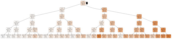
Figure 3.
Regression tree architecture for HALF.
Similarly, for day-ahead forecasting (DALF), the performance of the regression tree model that was developed to forecast the load L(T) based on features L(T-24), L(T-48), day and season status, temperature, and humidity was observed based on training and testing errors. The training and testing error metrics of the regression tree model are presented in Table 5 for DALF. From Table 5, it is observed that regression model with a depth “6” had lowest testing MSE, i.e., 0.00869 and was also well fitted without much difference between training and testing errors. Hence, the regression tree with a depth “6” was considered as the optimal model to deploy in a web application for day-ahead forecasting. The complete architecture of the regression tree with a depth “6” for day-ahead load forecasting is shown in Figure 4.
Table 5.
Training and testing errors of regression tree model for DALF.
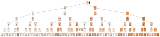
Figure 4.
Regression tree architecture for DALF.
The distribution of the predicted load with the regression tree model having a training MSE of 0.004 and a testing MSE of 0.005 was compared with actual load samples for the training and testing data for HALF and is presented in Figure 5. Similarly, the distribution of the predicted load with the regression tree model having a training MSE of 0.0065 and a testing MSE of 0.00869 was compared with actual load samples for the training and testing data for DALF and is presented in Figure 6. From Figure 5 and Figure 6, it is observed that most of the predicted and actual load samples are overlapping each other.
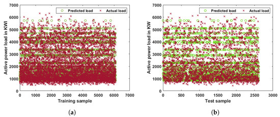
Figure 5.
Distribution of predicted and actual load samples with regression tree model for HALF. (a) Hour-ahead load forecasting: predicted load vs. actual load for training data. (b) Hour-ahead load forecasting: predicted load vs. actual load for testing data.
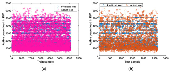
Figure 6.
Distribution of predicted and actual load samples with regression tree model for DALF. (a) Day-ahead load forecasting: predicted load vs. actual load for training data, (b) Day-ahead load forecasting: predicted load vs. actual load for testing data.
The predicted load using the regression tree model was compared with the actual load on 31 December 2021 and presented in Figure 7. From Figure 7, it is observed that the predicted load using the regression tree model is almost following the actual load curve during night time but has more differences during day time, and also that the predicted load is slightly further away from the actual load curve in the case of DALF in comparison with HALF. As in the first case, the load was predicted one day earlier, i.e., a 24 h time horizon.
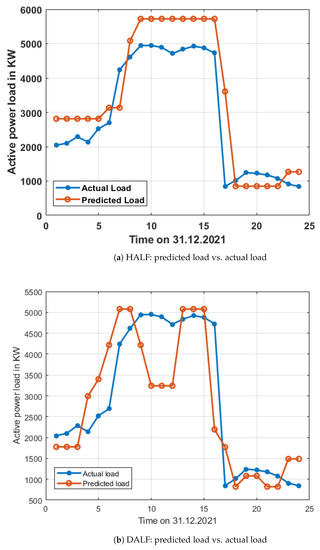
Figure 7.
Distribution of predicted and actual load samples with regression tree model on 31 December 2021.
A web application was developed using the optimal regression tree models to predict the load one hour ahead and one day ahead for a real-time usage as a prototype and is shown in Figure 8. This web application is accessible through the link https://loadforecasting-godishala-rt.herokuapp.com/, accessed on 1 May 2022 or through the QR code shown in Figure 8.

Figure 8.
Web application to predict active power load on a 33/11 kV substation in Godishala, Telangana State, India, developed using a regression tree model.
3.2. Impact of Season and Day on Regression Model Prediction
The forecasting performance of the trained machine learning model for HALF on various seasons, i.e., rainy, winter, and summer, is presented in Figure 9. From Figure 9, it is observed that the developed regression tree model is able to forecast the load with almost the same level of error (with very minor changes in error) for all seasons.
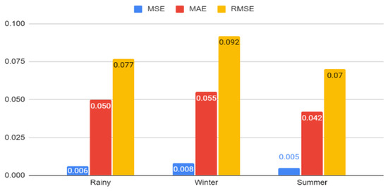
Figure 9.
Regression tree performance with respect to various seasons for HALF.
The forecasting performance of the trained machine learning model for HALF on various seasons, i.e., rainy, winter, and summer, is presented in Figure 10. From Figure 10, it is observed that the developed regression tree model is able to forecast the load with almost the same level of error irrespective of whether it is weekday or weekend.
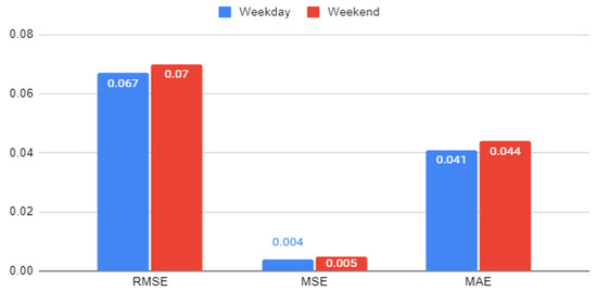
Figure 10.
Regression tree performance with respect to various day status for HALF.
3.3. Comparative Analysis
The performance of the machine learning model, i.e., the regression tree model, was compared with a linear regression model in terms of training and testing mean squared error for both HALF and DALF and presented in Figure 11. From Figure 11, it is observed that the regression tree model is forecasting the load with less error in comparison with the linear regression model for both HALF and DALF. In case of DALF, the model is forecasting the load with more error than HALF, as the latter one forecast the load just one hour ahead. The regression tree model is well fitted without much difference between training and testing errors.
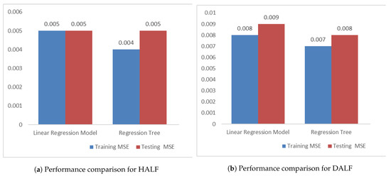
Figure 11.
Machine learning models performance comparison in terms of training and testing mean squared errors.
4. Conclusions
Electric power load forecasting one hour ahead and one day ahead are required for utilities to place a bid successfully in hour-ahead energy markets and day-ahead energy markets. In this paper, the active power on a 33/11 kV substation was predicted one hour ahead based on the load available in the last two hours and last two days at the time of prediction, and the day status, season status, temperature, and humidity. Similarly, the load was predicted one day ahead based on the load available in the last two days at the time of prediction, and the day status, season status, temperature, and humidity. A robust machine learning model was developed to forecast the load with good accuracy irrespective of the weather conditions and types of the day by incorporating features such as season, temperature, humidity, and day-status.
In this work, a machine learning model, i.e., a regression tree model was developed to predict the active power load on a 33/11 kV substation located in the Godishala village in Telangana State, India. Based on the results, it was observed that the regression tree model predicted the load one hour and one day ahead with less mean squared error in comparison with the linear regression model.
This work can be further extended by considering deep neural networks, sequence models, and conventional time series data prediction models. In this paper, the temperature and humidity data at the time of prediction were considered from an open-source website. However, we are currently further extending the model by integrating temperature and humidity forecasting models with the current load forecasting models.
Author Contributions
Conceptualization, V.V.; methodology, V.V.; software, V.V. and M.S.P.K.; validation, V.V.; formal analysis, V.V.; investigation, V.V.; resources, M.S.P.K.; data curation, M.S.P.K.; writing—original draft preparation, V.V.; writing—review and editing, V.V., M.S.P.K. and S.R.S.; visualization, V.V.; supervision, V.V.; project administration, V.V. All authors have read and agreed to the published version of the manuscript.
Funding
Woosong University’s Academic Research Funding—2022.
Institutional Review Board Statement
Not applicable.
Informed Consent Statement
Not applicable.
Data Availability Statement
Active power load data used to train and test machine learning models are available at https://data.mendeley.com/datasets/tj54nv46hj/1, accessed on 7 February 2022.
Conflicts of Interest
The authors declare no conflict of interest.
Abbreviations
The following abbreviations are used in this manuscript:
| L(T-1) | Active power load one hour before the time of prediction |
| L(T-2) | Active power load two hours before the time of prediction |
| L(T-24) | Active power load one day before the time of prediction |
| L(T-48) | Active power load two days before the time of prediction |
| L(T) | Active power load at hour “T” |
| MSE | Mean squared error |
| HALF | Hour-ahead load forecasting |
| DALF | Day-ahead load forecasting |
| RMSE | Root-mean-square error |
| MSE | Mean absolute error |
| Actual load at hour “T” | |
| Predicted load at hour “T” | |
| Number of training samples | |
| Number of testing samples |
Appendix A. Conversion of Continuous Data into Categorical Data
In this section, the step-by-step procedure that was used to build the regression tree model is presented. For this purpose, a sample dataset that was built from a few samples of the original dataset is shown in Table A1.
Table A1.
Sample data to build the regression tree.
Table A1.
Sample data to build the regression tree.
| L(T-24) | L(T-48) | DAY | SEASON | TEMP | HUMIDITY | L(T) |
|---|---|---|---|---|---|---|
| 2176 | 412 | 1 | 1 | 67 | 88 | 432 |
| 2354 | 1829 | 0 | 1 | 68 | 88 | 2260 |
| 2777 | 2647 | 0 | 2 | 70 | 83 | 2681 |
| 3112 | 3203 | 1 | 2 | 75 | 67 | 3343 |
| 1663 | 1549 | 1 | 0 | 75 | 73 | 1579 |
| 1010 | 1027 | 0 | 0 | 71 | 93 | 1018 |
To convert continuous features into categorical features, multiple subtables were formed from Table A1. Each subtable consisted of one input feature and one target feature. We sorted each subtable in ascending order of input feature in that table. We calculated the average between every two continuous input feature values. We converted continuous input features into categorical features based on their average value. We found the mean squared value for each average and the average value that gave lowest “MSE” were treated as threshold for that feature.
- Prepare the subtable for input feature L(T-24) and output feature L(T) as shown in Table A2.
Table A2.
Sorted subtable—L(T-24) vs. L(T).
Table A2.
Sorted subtable—L(T-24) vs. L(T).
| L(T-24) | L(T) |
|---|---|
| 1010 | 1018 |
| 1663 | 1579 |
| 2176 | 432 |
| 2354 | 2260 |
| 2777 | 2681 |
| 3112 | 3343 |
- Calculate the average between every two continuous input feature values for L(T-24) and the average values are [1336, 1919, 2265, 2566, 2945].
Table A3.
Categorical subtable—L(T-24) vs. L(T).
Table A3.
Categorical subtable—L(T-24) vs. L(T).
| L(T-24) | L(T) | (T) |
|---|---|---|
| <1336 | 1018 | 1018 |
| ≥1336 | 1579 | = 2059 |
| ≥1336 | 432 | 2059 |
| ≥1336 | 2260 | 2059 |
| ≥1336 | 2681 | 2059 |
| ≥1336 | 3343 | 2059 |
- Calculate the mean squared error based on the actual and predicted load values shown in Table A3 and presented below
= 825,622.
Table A4.
Categorical subtable—L(T-24) vs. L(T) with average value 1919.
Table A4.
Categorical subtable—L(T-24) vs. L(T) with average value 1919.
| L(T-24) | L(T) | (T) |
|---|---|---|
| <1919 | 1018 | 1298 |
| <1919 | 1579 | 1298 |
| ≥1919 | 432 | = 2179 |
| ≥1919 | 2260 | 2179 |
| ≥1919 | 2681 | 2179 |
| ≥1919 | 3343 | 2179 |
- Calculate the mean squared error based on the actual and predicted load values shown in Table A4 and presented below
= 803,903.
Table A5.
Categorical subtable—L(T-24) vs. L(T) with average value 2265.
Table A5.
Categorical subtable—L(T-24) vs. L(T) with average value 2265.
| L(T-24) | L(T) | (T) |
|---|---|---|
| <2265 | 1018 | = 1010 |
| <2265 | 1579 | 1010 |
| <2265 | 432 | 1010 |
| ≥2265 | 2260 | = 2761 |
| ≥2265 | 2681 | 2761 |
| ≥2265 | 3343 | 2761 |
- Calculate the mean squared error based on the actual and predicted load values shown in Table A5 and presented below
= 209,064.
Table A6.
Categorical subtable—L(T-24) vs. L(T) with average value 2566.
Table A6.
Categorical subtable—L(T-24) vs. L(T) with average value 2566.
| L(T-24) | L(T) | (T) |
|---|---|---|
| <2566 | 1018 | = 1322 |
| <2566 | 1579 | 1322 |
| <2566 | 432 | 1322 |
| <2566 | 2260 | 1322 |
| ≥2566 | 2681 | = 3012 |
| ≥2566 | 3343 | 3012 |
- Calculate the mean squared error based on the actual and predicted load values shown in Table A6 and presented below
= 341,675.
Table A7.
Categorical subtable—L(T-24) vs. L(T) with average value 2945.
Table A7.
Categorical subtable—L(T-24) vs. L(T) with average value 2945.
| L(T-24) | L(T) | (T) |
|---|---|---|
| <2945 | 1018 | = 1594 |
| <2945 | 1579 | 1594 |
| <2945 | 432 | 1594 |
| <2945 | 2260 | 1594 |
| <2945 | 2681 | 1594 |
| ≥2945 | 3343 | 3343 |
- Calculate the mean squared error based on the actual and predicted load values shown in Table A7 and presented below
= 551,591.
- Prepare subtable for input feature L(T-48) and output feature L(T) as shown in Table A8.
Table A8.
Sorted subtable—L(T-48) vs. L(T).
Table A8.
Sorted subtable—L(T-48) vs. L(T).
| L(T-48) | L(T) |
|---|---|
| 412 | 432 |
| 1027 | 1018 |
| 1549 | 1579 |
| 1829 | 2260 |
| 2647 | 2681 |
| 3203 | 3343 |
- Calculate the average between every two continuous input feature values for L(T-48) and the average values are [720, 1288, 1689, 2238, 2925].
Table A9.
Categorical subtable—L(T-48) vs. L(T).
Table A9.
Categorical subtable—L(T-48) vs. L(T).
| L(T-48) | L(T) | (T) |
|---|---|---|
| <720 | 432 | 432 |
| ≥720 | 1018 | = 2176.2 |
| ≥720 | 1579 | 2176.2 |
| ≥720 | 2260 | 2176.2 |
| ≥720 | 2681 | 2176.2 |
| ≥720 | 3343 | 2176.2 |
- Calculate the mean squared error based on the actual and predicted load values shown in Table A9 and presented below
= 553,557.1333.
Table A10.
Categorical subtable—L(T-48) vs. L(T).
Table A10.
Categorical subtable—L(T-48) vs. L(T).
| L(T-48) | L(T) | (T) |
|---|---|---|
| <1288 | 432 | = 725 |
| <1288 | 1018 | 725 |
| ≥1288 | 1579 | = 2465.75 |
| ≥1288 | 2260 | 2465.75 |
| ≥1288 | 2681 | 2465.75 |
| ≥1288 | 3343 | 2465.75 |
- Calculate the mean squared error based on the actual and predicted load values shown in Table A10 and presented below
= 302,709.4583.
Table A11.
Categorical subtable—L(T-48) vs. L(T).
Table A11.
Categorical subtable—L(T-48) vs. L(T).
| L(T-48) | L(T) | (T) |
|---|---|---|
| <1689 | 432 | = 1009.666667 |
| <1689 | 1018 | 1009.666667 |
| <1689 | 1579 | 1009.666667 |
| ≥1689 | 2260 | = 2761.333333 |
| ≥1689 | 2681 | 2761.333333 |
| ≥1689 | 3343 | 2761.333333 |
- Calculate the mean squared error based on the actual and predicted load values shown in Table A11 and presented below
= 209,005.5556.
Table A12.
Categorical subtable—L(T-48) vs. L(T).
Table A12.
Categorical subtable—L(T-48) vs. L(T).
| L(T-48) | L(T) | (T) |
|---|---|---|
| <2238 | 432 | = 1322.25 |
| <2238 | 1018 | 1322.257 |
| <2238 | 1579 | 1322.25 |
| <2238 | 2260 | 1322.25 |
| ≥2238 | 2681 | = 3012 |
| ≥2238 | 3343 | 3012 |
- Calculate the mean squared error based on the actual and predicted load values shown in Table A12 and presented below
= 341,588.4583.
Table A13.
Categorical subtable—L(T-48) vs. L(T).
Table A13.
Categorical subtable—L(T-48) vs. L(T).
| L(T-48) | L(T) | (T) |
|---|---|---|
| <2925 | 432 | = 1594 |
| <2925 | 1018 | 1594 |
| <2925 | 1579 | 1594 |
| <2925 | 2260 | 1594 |
| <2925 | 2681 | 1594 |
| ≥2925 | 3343 | 3343 |
- Calculate the mean squared error based on the actual and predicted load values shown in Table A13 and presented below
= 551,228.3333.
- Prepare subtable for input feature L(TEMP) and output feature L(T) and shown in Table A14
Table A14.
Sorted subtable—L(TEMP) vs. L(T).
Table A14.
Sorted subtable—L(TEMP) vs. L(T).
| L(TEMP) | L(T) |
|---|---|
| 67 | 432 |
| 68 | 2260 |
| 70 | 2681 |
| 71 | 1018 |
| 75 | 3343 |
| 75 | 1579 |
- Calculate average between every two continuous input feature values for L(TEMP) and the average values are [67.5, 69, 70.5, 73, 75].
Table A15.
Categorical subtable—L(TEMP) vs. L(T).
Table A15.
Categorical subtable—L(TEMP) vs. L(T).
| L(TEMP) | L(T) | (T) |
|---|---|---|
| <67.5 | 432 | 432 |
| ≥67.5 | 2260 | = 2176.2 |
| ≥67.5 | 2681 | 2176.2 |
| ≥67.5 | 1018 | 2176.2 |
| ≥67.5 | 3343 | 2176.2 |
| ≥67.5 | 1579 | 2176.2 |
- Calculate the mean squared error based on the actual and predicted load values shown in Table A15 and presented below
= 553,557.
Table A16.
Categorical subtable—L(TEMP) vs. L(T).
Table A16.
Categorical subtable—L(TEMP) vs. L(T).
| L(TEMP) | L(T) | (T) |
|---|---|---|
| <69 | 432 | = 1346 |
| <69 | 2260 | 1346 |
| ≥69 | 2681 | = 2155.25 |
| ≥69 | 1018 | 2155.25 |
| ≥69 | 3343 | 2155.25 |
| ≥69 | 1579 | 2155.25 |
- Calculate the mean squared error based on the actual and predicted load values shown in Table A16 and presented below
= 830,559.
Table A17.
Categorical subtable—L(TEMP) vs. L(T).
Table A17.
Categorical subtable—L(TEMP) vs. L(T).
| L(TEMP) | L(T) | (T) |
|---|---|---|
| <70.5 | 432 | = 1791 |
| <70.5 | 2260 | 1791 |
| <70.5 | 2681 | 1791 |
| ≥70.5 | 1018 | = 1980 |
| ≥70.5 | 3343 | 1980 |
| ≥70.5 | 1579 | 1980 |
- Calculate the mean squared error based on the actual and predicted load values shown in Table A17 and presented below
= 967,159.
Table A18.
Categorical subtable—L(TEMP) vs. L(T).
Table A18.
Categorical subtable—L(TEMP) vs. L(T).
| L(TEMP) | L(T) | (T) |
|---|---|---|
| <73 | 432 | = 1597.75 |
| <73 | 2260 | 1597.75 |
| <73 | 2681 | 1597.75 |
| <73 | 1018 | 1597.75 |
| ≥73 | 3343 | = 2461 |
| ≥73 | 1579 | 2461 |
- Calculate the mean squared error based on the actual and predicted load values shown in Table A18 and presented below
= 810,489.
Table A19.
Categorical subtable—L(TEMP) vs. L(T).
Table A19.
Categorical subtable—L(TEMP) vs. L(T).
| L(TEMP) | L(T) | (T) |
|---|---|---|
| <75 | 432 | = 1946.8 |
| <75 | 2260 | 1946.8 |
| <75 | 2681 | 1946.8 |
| <75 | 1018 | 1946.8 |
| <75 | 3343 | 1946.8 |
| ≥75 | 1579 | 1579 |
- Calculate the mean squared error based on the actual and predicted load values shown in Table A19 and presented below
= 957,301.
- Prepare subtable for input feature Humidity and output feature L(T) and shown in Table A20
Table A20.
Sorted subtable—Humidity vs. L(T).
Table A20.
Sorted subtable—Humidity vs. L(T).
| Humidity | L(T) |
|---|---|
| 67 | 3343 |
| 73 | 1579 |
| 83 | 2681 |
| 88 | 432 |
| 88 | 2260 |
| 93 | 1018 |
- Calculate average between every two continuous input feature values for Humidity and the average values are [70, 78, 85.5, 88, 90.5].
Table A21.
Categorical subtable—Humidity vs. L(T).
Table A21.
Categorical subtable—Humidity vs. L(T).
| Humidity | L(T) | (T) |
|---|---|---|
| <70 | 3343 | 3343 |
| ≥70 | 1579 | = 1594 |
| ≥70 | 2681 | 1594 |
| ≥70 | 432 | 1594 |
| ≥70 | 2260 | 1594 |
| ≥70 | 1018 | 1594 |
- Calculate the mean squared error based on the actual and predicted load values shown in Table A21 and presented below
= 551,228.
Table A22.
Categorical subtable—Humidity vs. L(T).
Table A22.
Categorical subtable—Humidity vs. L(T).
| Humidity | L(T) | (T) |
|---|---|---|
| <78 | 3343 | = 2461 |
| <78 | 1579 | 2461 |
| ≥78 | 2681 | = 1597.75 |
| ≥78 | 432 | 1597.75 |
| ≥78 | 2260 | 1597.75 |
| ≥78 | 1018 | 1597.75 |
- Calculate the mean squared error based on the actual and predicted load values shown in Table A22 and presented below
= 810,489.
Table A23.
Categorical subtable—Humidity vs. L(T).
Table A23.
Categorical subtable—Humidity vs. L(T).
| Humidity | L(T) | (T) |
|---|---|---|
| <85.5 | 3343 | = 2534.33 |
| <85.5 | 1579 | 2534.33 |
| <85.5 | 2681 | 2534.33 |
| ≥85.5 | 432 | = 1236.67 |
| ≥85.5 | 2260 | 1236.67 |
| ≥85.5 | 1018 | 1236.67 |
- Calculate the mean squared error based on the actual and predicted load values shown in Table A23 and presented below
= 555,105
Table A24.
Categorical subtable—Humidity vs. L(T).
Table A24.
Categorical subtable—Humidity vs. L(T).
| Humidity | L(T) | (T) |
|---|---|---|
| <88 | 3343 | = 2008.75 |
| <88 | 1579 | 2008.75 |
| <88 | 2681 | 2008.75 |
| <88 | 432 | 2008.75 |
| ≥88 | 2260 | = 1639 |
| ≥88 | 1018 | 1639 |
- Calculate the mean squared error based on the actual and predicted load values shown in Table A24 and presented below
= 945,708
Table A25.
Categorical subtable—Humidity vs. L(T).
Table A25.
Categorical subtable—Humidity vs. L(T).
| Humidity | L(T) | (T) |
|---|---|---|
| <90.5 | 3343 | = 2059 |
| <90.5 | 1579 | 2059 |
| <90.5 | 2681 | 2059 |
| <90.5 | 432 | 2059 |
| <90.5 | 2260 | 2059 |
| ≥90.5 | 1018 | 1018 |
- Calculate the mean squared error based on the actual and predicted load values shown in Table A25 and presented below
= 825,578
From all the above calculations, the minimum MSE value for the feature “T-24” is 209,064 for the split ≥2265, the minimum MSE value for the feature “T-48” is 209,006 for the split ≥1689, the minimum MSE value for the feature “Temperature” is 553,557 for the split ≥67.5, the minimum MSE value for the feature “Humidity” is 551,228 for the split ≥70. Hence, these splits against each feature were used to convert the continuous data shown in Table A1 into categorical data, as shown in Table A26. Furthermore, the MSE value for the day with categories (1 and 0) is 965,922 and the MSE value for the season with categories (0, 1, and 2) is 747157. All the MSE values are presented in Table A1 with bold font.
Table A26.
Sample categorical data to build regression tree.
Table A26.
Sample categorical data to build regression tree.
| L(T-24) | L(T-48) | DAY | SEASON | TEMP | HUMIDITY | L(T) |
|---|---|---|---|---|---|---|
| <2265 | <1689 | 1 | 1 | <67.5 | ≥70 | 432 |
| ≥2265 | ≥1689 | 0 | 1 | ≥67.5 | ≥70 | 2260 |
| ≥2265 | ≥1689 | 0 | 2 | ≥67.5 | ≥70 | 2681 |
| ≥2265 | ≥1689 | 1 | 2 | ≥67.5 | <70 | 3343 |
| <2265 | <1689 | 1 | 0 | ≥67.5 | ≥70 | 1579 |
| <2265 | <1689 | 0 | 0 | ≥67.5 | ≥70 | 1018 |
| 209,064 | 209,006 | 965,922 | 747,157 | 553,557 | 551,228 | – |
Appendix B. Regression Tree Model Formulation
From Table A26, we observe that L(T-48) has a minimum MSE value, i.e., 209,006 in comparison with all the remaining features. Hence, the input feature L(T-48) is considered as a root node for the regression tree and that node has two branches ≥1689 and <1689. In order to identify the decision node under each branch, Table A26 is divided into two subtables, presented in Table A27 and Table A28.
Table A27.
Subtable: L(T-48) < 1689.
Table A27.
Subtable: L(T-48) < 1689.
| L(T-24) | DAY | SEASON | TEMP | HUMIDITY | T |
|---|---|---|---|---|---|
| <2265 | 1 | 1 | <67.5 | ≥70 | 432 |
| <2265 | 1 | 0 | ≥67.5 | ≥70 | 1579 |
| <2265 | 0 | 0 | ≥67.5 | ≥70 | 1018 |
Table A28.
Subtable: L(T-48) ≥ 1689.
Table A28.
Subtable: L(T-48) ≥ 1689.
| L(T-24) | DAY | SEASON | TEMP | HUMIDITY | T |
|---|---|---|---|---|---|
| ≥2265 | 0 | 1 | ≥67.5 | ≥70 | 2260 |
| ≥2265 | 0 | 2 | ≥67.5 | ≥70 | 2681 |
| ≥2265 | 1 | 2 | ≥67.5 | <70 | 3343 |
- In order to identify the decision node among L(T-24), day, season, temperature, and humidity under branch <1689 Table A28 is further divided into multiple subtables based on each input feature.
Table A29.
L(T-24) vs. L(T) for L(T-48) < 1689.
Table A29.
L(T-24) vs. L(T) for L(T-48) < 1689.
| L(T-24) | L(T) Prediction | Squared Error | MSE | |
|---|---|---|---|---|
| <2265 | 432 | 1010 | 333,699 | |
| <2265 | 1579 | 1010 | 324,140 | 219,303 |
| <2265 | 1018 | 1010 | 69 |
Table A30.
Day vs. L(T) for L(T-48) < 1689.
Table A30.
Day vs. L(T) for L(T-48) < 1689.
| Day | L(T) Prediction | Squared Error | MSE | |
|---|---|---|---|---|
| 1 | 432 | 1005.5 | 328,902.25 | |
| 1 | 1579 | 1005.5 | 328,902.25 | 219,268 |
| 0 | 1018 | 1018 | 0 |
Table A31.
Season vs. L(T) for L(T-48) < 1689.
Table A31.
Season vs. L(T) for L(T-48) < 1689.
| Season | L(T) Prediction | Squared Error | MSE | |
|---|---|---|---|---|
| 1 | 432 | 432 | 0 | |
| 0 | 1579 | 1298.5 | 78,680.25 | 52,454 |
| 0 | 1018 | 1298.5 | 78,680.25 |
Table A32.
Temperature vs. L(T) for L(T-48) < 1689.
Table A32.
Temperature vs. L(T) for L(T-48) < 1689.
| Temperature | L(T) Prediction | Squared Error | MSE | |
|---|---|---|---|---|
| <67.5 | 432 | 432 | 0 | |
| ≥67.5 | 1579 | 1298.5 | 78,680.25 | 52454 |
| ≥67.5 | 1018 | 1298.5 | 78,680.25 |
Table A33.
Humidity vs. L(T) for L(T-48) < 1689.
Table A33.
Humidity vs. L(T) for L(T-48) < 1689.
| Humidity | L(T) Prediction | Squared Error | MSE | |
|---|---|---|---|---|
| ≥70 | 432 | 1009.67 | 333,698.78 | |
| ≥70 | 1579 | 1009.67 | 324,140.44 | 219,303 |
| ≥70 | 1018 | 1009.67 | 69.44 |
It is observed from the above calculations that season and temperature have a minimum MSE, i.e., 52,454. Here, season is considered as a decision node under branch L(T-48) < 1689. Now, the node season has two branches, i.e., season “1” and “0”. In order to identify the decision/leaf node under each branch, Table A27 is divided into two subtables, presented in Table A34 and Table A35. From Table A34, it is observed that the branch corresponding to season “1” has a leaf node with value 432.
Table A34.
Subtable: L(T-48) < 1689 and season = “1”.
Table A34.
Subtable: L(T-48) < 1689 and season = “1”.
| T-24 | DAY | TEMP | HUMIDITY | T |
|---|---|---|---|---|
| <2265 | 1 | <67.5 | ≥70 | 432 |
Table A35.
Subtable: L(T-48) < 1689 and season = “0”.
Table A35.
Subtable: L(T-48) < 1689 and season = “0”.
| T-24 | DAY | TEMP | HUMIDITY | T |
|---|---|---|---|---|
| <2265 | 1 | ≥67.5 | ≥70 | 1579 |
| <2265 | 0 | ≥67.5 | ≥70 | 1018 |
In order to identify the decision node among L(T-24), day, temperature, and humidity under branch season “0”, Table A35 is divided into multiple subtables with respect to each feature.
Table A36.
L(T-24) vs. L(T) for L(T-48) < 1689 and season “0”.
Table A36.
L(T-24) vs. L(T) for L(T-48) < 1689 and season “0”.
| L(T-24) | L(T) | Prediction | Squared Error | MSE |
|---|---|---|---|---|
| <2265 | 1579 | 1298.5 | 78,680 | 78,680 |
| <2265 | 1018 | 1298.5 | 78,680 |
Table A37.
Day vs. L(T) for L(T-48) < 1689 and season “0”.
Table A37.
Day vs. L(T) for L(T-48) < 1689 and season “0”.
| Day | L(T) | Prediction | Squared Error | MSE |
|---|---|---|---|---|
| 1 | 1579 | 1579 | 0 | 0 |
| 0 | 1018 | 1018 | 0 |
Table A38.
Temperature vs. L(T) for L(T-48) < 1689 and season “0”.
Table A38.
Temperature vs. L(T) for L(T-48) < 1689 and season “0”.
| Temperature | L(T) | Prediction | Squared Error | MSE |
|---|---|---|---|---|
| ≥67.5 | 1579 | 1298.5 | 78,680 | 78,680 |
| ≥67.5 | 1018 | 1298.5 | 78,680 |
Table A39.
Humidity vs. L(T) for L(T-48) < 1689 and season “0”.
Table A39.
Humidity vs. L(T) for L(T-48) < 1689 and season “0”.
| Humidity | L(T) | Prediction | Squared Error | MSE |
|---|---|---|---|---|
| ≥70 | 1579 | 1298.5 | 78,680 | 78,680 |
| ≥70 | 1018 | 1298.5 | 78,680 |
It is observed from the above calculations that feature “Day” has a minimum MSE, i.e., 0. Here, “Day” is considered as decision node under the season “0” branch. Now, node “Day” has two branches, i.e., day “0” and “1” as presented in Table A37. From Table A37, it is observed that the branch corresponding to day “1” has a leaf node with value 1579 and day “0” has a leaf node with value 1018.
- In order to identify the decision node among L(T-24), day, season, temperature, and humidity under branch ≥1689, Table A40 is further divided into multiple subtables based on each input feature.
Table A40.
L(T-24) vs. L(T) for L(T-48) ≥ 1689.
Table A40.
L(T-24) vs. L(T) for L(T-48) ≥ 1689.
| L(T-24) | L(T) | Prediction | Squared Error | MSE |
|---|---|---|---|---|
| ≥2265 | 2260 | 2761.33 | 251,335 | |
| ≥2265 | 2681 | 2761.33 | 6453 | 198,708 |
| ≥2265 | 3343 | 2761.33 | 338,336 |
Table A41.
Day vs. L(T) for L(T-48) ≥ 1689.
Table A41.
Day vs. L(T) for L(T-48) ≥ 1689.
| Day | L(T) Prediction | Squared Error | MSE | |
|---|---|---|---|---|
| 0 | 2260 | 2470.5 | 44310 | |
| 0 | 2681 | 2470.5 | 44310 | 29,540 |
| 1 | 3343 | 3343 | 0 |
Table A42.
Season vs. L(T) for L(T-48) ≥ 1689.
Table A42.
Season vs. L(T) for L(T-48) ≥ 1689.
| Season | L(T) Prediction | Squared Error | MSE | |
|---|---|---|---|---|
| 1 | 2260 | 2260 | 0 | |
| 2 | 2681 | 3012 | 109,561 | 73,041 |
| 2 | 3343 | 3012 | 109,561 |
Table A43.
Temperature vs. L(T) for L(T-48) ≥ 1689.
Table A43.
Temperature vs. L(T) for L(T-48) ≥ 1689.
| Temperature | L(T) Prediction | Squared Error | MSE | |
|---|---|---|---|---|
| ≥67.5 | 2260 | 2761.33 | 251,335 | |
| ≥67.5 | 2681 | 2761.33 | 6453 | 198,708 |
| ≥67.5 | 3343 | 2761.33 | 338,336 |
Table A44.
Humidity vs. L(T) for L(T-48) ≥ 1689.
Table A44.
Humidity vs. L(T) for L(T-48) ≥ 1689.
| Humidity | L(T) Prediction | Squared Error | MSE | |
|---|---|---|---|---|
| ≥70 | 2260 | 2470.5 | 44310 | |
| ≥70 | 2681 | 2470.5 | 44310 | 29,540 |
| <67.5 | 3343 | 3343 | 0 |
It is observed from the above calculations that day and humidity have a minimum MSE, i.e., 29,540. Here, day is considered as a decision node under branch L(T-48) ≥ 1689. Now, the node day has two branches, i.e., day “1” and “0”. In order to identify the decision/leaf node under each branch, Table A28 is divided into two subtables, as presented in Table A45 and in Table A46. From Table A45, it is observed that the branch corresponding to day “1” has a leaf node with value 3343.
Table A45.
Subtable: L(T-48) ≥ 1689 and day = “1”.
Table A45.
Subtable: L(T-48) ≥ 1689 and day = “1”.
| L(T-24) | SEASON | TEMP | HUMIDITY | L(T) |
|---|---|---|---|---|
| ≥2265 | 2 | ≥67.5 | <70 | 3343 |
Table A46.
Subtable: L(T-48) ≥ 1689 and Day = “0”.
Table A46.
Subtable: L(T-48) ≥ 1689 and Day = “0”.
| L(T-24) | SEASON | TEMP | HUMIDITY | L(T) |
|---|---|---|---|---|
| ≥2265 | 1 | ≥67.5 | ≥70 | 2260 |
| ≥2265 | 2 | ≥67.5 | ≥70 | 2681 |
In order to identify the decision node among L(T-24), season, temperature, and humidity under the branch day “0”, Table A46 is divided into multiple subtables with respect to each feature.
Table A47.
L(T-24) vs. L(T) for L(T-48) ≥ 1689 and day “0”.
Table A47.
L(T-24) vs. L(T) for L(T-48) ≥ 1689 and day “0”.
| L(T-24) | L(T) | Prediction | Squared Error | MSE |
|---|---|---|---|---|
| ≥2265 | 2260 | 2470.5 | 44,310.25 | 44,310.25 |
| ≥2265 | 2681 | 2470.5 | 44,310.25 |
Table A48.
Season vs. L(T) for L(T-48) ≥ 1689 and day “0”.
Table A48.
Season vs. L(T) for L(T-48) ≥ 1689 and day “0”.
| Season | L(T) | Prediction | Squared Error | MSE |
|---|---|---|---|---|
| 1 | 2260 | 2260 | 0 | 0 |
| 2 | 2681 | 2681 | 0 |
Table A49.
Temperature vs. L(T) for L(T-48) ≥ 1689 and day “0”.
Table A49.
Temperature vs. L(T) for L(T-48) ≥ 1689 and day “0”.
| Temperature | L(T) | Prediction | Squared Error | MSE |
|---|---|---|---|---|
| ≥67.5 | 2260 | 2470.5 | 44,310.25 | 44,310.25 |
| ≥67.5 | 2681 | 2470.5 | 44,310.25 |
Table A50.
Humidity vs. L(T) for L(T-48) ≥ 1689 and day “0”.
Table A50.
Humidity vs. L(T) for L(T-48) ≥ 1689 and day “0”.
| Humidity | L(T) | Prediction | Squared Error | MSE |
|---|---|---|---|---|
| ≥70 | 2260 | 2470.5 | 44,310.25 | 44,310.25 |
| ≥70 | 2681 | 2470.5 | 44,310.25 |
It is observed from the above calculations that feature “Season” has a minimum MSE, i.e., 0. Here, “Season” is considered as a decision node under branch day “0”. Now node “Season” has two branches, i.e., season “1” and “2” as presented in Table A48. From Table A48, it is observed that the branch corresponding to season “1” has a leaf node with value 2260 and season “2” has a leaf node with value 2681. Finally, the complete decision tree to predict load L(T) based on the features, i.e., L(T-24), L(T-48), day, season, temperature, and humidity is shown in Figure A1. The decision tree shown in Figure A1 was used to predict the load shown in Table A1 and the predicted load is shown in Table A51. From Table A51, it is observed that both actual and predicted load values are equal.
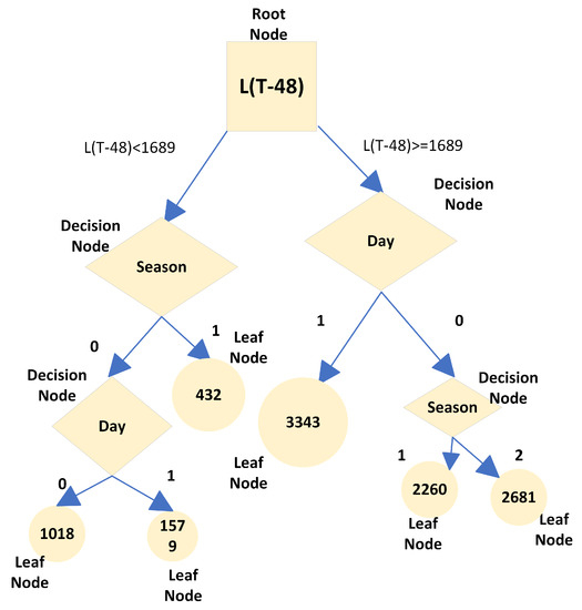
Figure A1.
Regression tree architecture with sample data.
Table A51.
Predicted load from sample data using regression tree.
Table A51.
Predicted load from sample data using regression tree.
| L(T-24) | L(T-48) | DAY | SEASON | TEMP | HUMIDITY | L(T) | (T) |
|---|---|---|---|---|---|---|---|
| 2176 | 412 | 1 | 1 | 67 | 88 | 432 | 432 |
| 2354 | 1829 | 0 | 1 | 68 | 88 | 2260 | 2260 |
| 2777 | 2647 | 0 | 2 | 70 | 83 | 2681 | 2681 |
| 3112 | 3203 | 1 | 2 | 75 | 67 | 3343 | 3343 |
| 1663 | 1549 | 1 | 0 | 75 | 73 | 1579 | 1579 |
| 1010 | 1027 | 0 | 0 | 71 | 93 | 1018 | 1018 |
References
- Kersting, W.H. Distribution System Modeling and Analysis; CRC Press: Boca Raton, FL, USA, 2018. [Google Scholar]
- Willis, H.L. Spatial Electric Load Forecasting; CRC Press: Boca Raton, FL, USA, 2002. [Google Scholar]
- Henselmeyer, S.; Grzegorzek, M. Short-Term Load Forecasting Using an Attended Sequential Encoder-Stacked Decoder Model with Online Training. Appl. Sci. 2021, 11, 4927. [Google Scholar] [CrossRef]
- Shohan, M.J.A.; Faruque, M.O.; Foo, S.Y. Forecasting of Electric Load Using a Hybrid LSTM-Neural Prophet Model. Energies 2022, 15, 2158. [Google Scholar] [CrossRef]
- Grzeszczyk, T.A.; Grzeszczyk, M.K. Justifying Short-Term Load Forecasts Obtained with the Use of Neural Models. Energies 2022, 15, 1852. [Google Scholar] [CrossRef]
- Kiprijanovska, I.; Stankoski, S.; Ilievski, I.; Jovanovski, S.; Gams, M.; Gjoreski, H. Houseec: Day-ahead household electrical energy consumption forecasting using deep learning. Energies 2020, 13, 2672. [Google Scholar] [CrossRef]
- Shah, I.; Iftikhar, H.; Ali, S.; Wang, D. Short-term electricity demand forecasting using components estimation technique. Energies 2019, 12, 2532. [Google Scholar] [CrossRef] [Green Version]
- Jiang, H.; Zhang, Y.; Muljadi, E.; Zhang, J.J.; Gao, D.W. A short-term and high-resolution distribution system load forecasting approach using support vector regression with hybrid parameters optimization. IEEE Trans. Smart Grid 2016, 9, 3341–3350. [Google Scholar] [CrossRef]
- Zhang, Z.; Dou, C.; Yue, D.; Zhang, B. Predictive voltage hierarchical controller design for islanded microgrids under limited communication. IEEE Trans. Circuits Syst. I Regul. Pap. 2021, 69, 933–945. [Google Scholar] [CrossRef]
- Zhang, Z.; Mishra, Y.; Yue, D.; Dou, C.; Zhang, B.; Tian, Y.C. Delay-tolerant predictive power compensation control for photovoltaic voltage regulation. IEEE Trans. Ind. Inform. 2020, 17, 4545–4554. [Google Scholar] [CrossRef]
- Hong, T.; Fan, S. Probabilistic electric load forecasting: A tutorial review. Int. J. Forecast. 2016, 32, 914–938. [Google Scholar] [CrossRef]
- Fallah, S.N.; Ganjkhani, M.; Shamshirband, S.; Chau, K.w. Computational intelligence on short-term load forecasting: A methodological overview. Energies 2019, 12, 393. [Google Scholar] [CrossRef] [Green Version]
- Veeramsetty, V.; Deshmukh, R. Electric power load forecasting on a 33/11 kV substation using artificial neural networks. SN Appl. Sci. 2020, 2, 855. [Google Scholar] [CrossRef] [Green Version]
- Veeramsetty, V.; Mohnot, A.; Singal, G.; Salkuti, S.R. Short term active power load prediction on a 33/11 kv substation using regression models. Energies 2021, 14, 2981. [Google Scholar] [CrossRef]
- Veeramsetty, V.; Chandra, D.R.; Salkuti, S.R. Short-term electric power load forecasting using factor analysis and long short-term memory for smart cities. Int. J. Circuit Theory Appl. 2021, 49, 1678–1703. [Google Scholar] [CrossRef]
- Veeramsetty, V.; Reddy, K.R.; Santhosh, M.; Mohnot, A.; Singal, G. Short-term electric power load forecasting using random forest and gated recurrent unit. Electr. Eng. 2022, 104, 307–329. [Google Scholar] [CrossRef]
- Veeramsetty, V.; Rakesh Chandra, D.; Salkuti, S.R. Short Term Active Power Load Forecasting Using Machine Learning with Feature Selection. In Next Generation Smart Grids: Modeling, Control and Optimization; Springer: Berlin/Heidelberg, Germany, 2022; pp. 103–124. [Google Scholar]
- Veeramsetty, V.; Chandra, D.R.; Grimaccia, F.; Mussetta, M. Short Term Electric Power Load Forecasting Using Principal Component Analysis and Recurrent Neural Networks. Forecasting 2022, 4, 149–164. [Google Scholar] [CrossRef]
- Chemetova, S.; Santos, P.; Ventim-Neves, M. Load forecasting in electrical distribution grid of medium voltage. In Proceedings of the Doctoral Conference on Computing, Electrical and Industrial Systems, Costa de Caparica, Portugal, 11–13 April 2016; Springer: Berlin/Heidelberg, Germany, 2016; pp. 340–349. [Google Scholar]
- Couraud, B.; Roche, R. A distribution loads forecast methodology based on transmission grid substations SCADA Data. In Proceedings of the 2014 IEEE Innovative Smart Grid Technologies-Asia (ISGT ASIA), Kuala Lumpur, Malaysia, 20–23 May 2014; pp. 35–40. [Google Scholar]
- Andriopoulos, N.; Magklaras, A.; Birbas, A.; Papalexopoulos, A.; Valouxis, C.; Daskalaki, S.; Birbas, M.; Housos, E.; Papaioannou, G.P. Short term electric load forecasting based on data transformation and statistical machine learning. Appl. Sci. 2020, 11, 158. [Google Scholar] [CrossRef]
- Boriratrit, S.; Srithapon, C.; Fuangfoo, P.; Chatthaworn, R. Metaheuristic Extreme Learning Machine for Improving Performance of Electric Energy Demand Forecasting. Computers 2022, 11, 66. [Google Scholar] [CrossRef]
- Wang, Y.; Liu, M.; Bao, Z.; Zhang, S. Short-Term Load Forecasting with Multi-Source Data Using Gated Recurrent Unit Neural Networks. Energies 2018, 11, 1138. [Google Scholar] [CrossRef] [Green Version]
- Li, Y.; Huang, Y.; Zhang, M. Short-Term Load Forecasting for Electric Vehicle Charging Station Based on Niche Immunity Lion Algorithm and Convolutional Neural Network. Energies 2018, 11, 1253. [Google Scholar] [CrossRef] [Green Version]
- Hu, Z.; Ma, J.; Yang, L.; Li, X.; Pang, M. Decomposition-Based Dynamic Adaptive Combination Forecasting for Monthly Electricity Demand. Sustainability 2019, 11, 1272. [Google Scholar] [CrossRef] [Green Version]
- Amoasi Acquah, M.; Kodaira, D.; Han, S. Real-Time Demand Side Management Algorithm Using Stochastic Optimization. Energies 2018, 11, 1166. [Google Scholar] [CrossRef] [Green Version]
- Nagbe, K.; Cugliari, J.; Jacques, J. Short-Term Electricity Demand Forecasting Using a Functional State Space Model. Energies 2018, 11, 1120. [Google Scholar] [CrossRef] [Green Version]
- Kiptoo, M.K.; Adewuyi, O.B.; Lotfy, M.E.; Amara, T.; Konneh, K.V.; Senjyu, T. Assessing the techno-economic benefits of flexible demand resources scheduling for renewable energy–based smart microgrid planning. Future Internet 2019, 11, 219. [Google Scholar] [CrossRef] [Green Version]
- Yu, J.; Park, J.H.; Kim, S. A New Input Selection Algorithm Using the Group Method of Data Handling and Bootstrap Method for Support Vector Regression Based Hourly Load Forecasting. Energies 2018, 11, 2870. [Google Scholar] [CrossRef] [Green Version]
- Kampelis, N.; Tsekeri, E.; Kolokotsa, D.; Kalaitzakis, K.; Isidori, D.; Cristalli, C. Development of demand response energy management optimization at building and district levels using genetic algorithm and artificial neural network modelling power predictions. Energies 2018, 11, 3012. [Google Scholar] [CrossRef] [Green Version]
- Jin, X.B.; Zheng, W.Z.; Kong, J.L.; Wang, X.Y.; Bai, Y.T.; Su, T.L.; Lin, S. Deep-learning forecasting method for electric power load via attention-based encoder-decoder with bayesian optimization. Energies 2021, 14, 1596. [Google Scholar] [CrossRef]
- Han, M.; Zhong, J.; Sang, P.; Liao, H.; Tan, A. A Combined Model Incorporating Improved SSA and LSTM Algorithms for Short-Term Load Forecasting. Electronics 2022, 11, 1835. [Google Scholar] [CrossRef]
- Taleb, I.; Guerard, G.; Fauberteau, F.; Nguyen, N. A Flexible Deep Learning Method for Energy Forecasting. Energies 2022, 15, 3926. [Google Scholar] [CrossRef]
- Aldhyani, T.H.; Alkahtani, H. A bidirectional long short-term memory model algorithm for predicting COVID-19 in gulf countries. Life 2021, 11, 1118. [Google Scholar] [CrossRef]
- Zhang, W.; Wu, P.; Peng, Y.; Liu, D. Roll motion prediction of unmanned surface vehicle based on coupled CNN and LSTM. Future Internet 2019, 11, 243. [Google Scholar] [CrossRef] [Green Version]
- Lu, Y.; Li, Y.; Xie, D.; Wei, E.; Bao, X.; Chen, H.; Zhong, X. The application of improved random forest algorithm on the prediction of electric vehicle charging load. Energies 2018, 11, 3207. [Google Scholar] [CrossRef] [Green Version]
- Maitah, M.; Malec, K.; Ge, Y.; Gebeltová, Z.; Smutka, L.; Blažek, V.; Pánková, L.; Maitah, K.; Mach, J. Assessment and Prediction of Maize Production Considering Climate Change by Extreme Learning Machine in Czechia. Agronomy 2021, 11, 2344. [Google Scholar] [CrossRef]
- López-Espinoza, E.D.; Zavala-Hidalgo, J.; Mahmood, R.; Gómez-Ramos, O. Assessing the impact of land use and land cover data representation on weather forecast quality: A case study in central mexico. Atmosphere 2020, 11, 1242. [Google Scholar] [CrossRef]
- Hevia-Montiel, N.; Perez-Gonzalez, J.; Neme, A.; Haro, P. Machine Learning-Based Feature Selection and Classification for the Experimental Diagnosis of Trypanosoma cruzi. Electronics 2022, 11, 785. [Google Scholar] [CrossRef]
- Alaoui, A.; Hallama, M.; Bär, R.; Panagea, I.; Bachmann, F.; Pekrun, C.; Fleskens, L.; Kandeler, E.; Hessel, R. A New Framework to Assess Sustainability of Soil Improving Cropping Systems in Europe. Land 2022, 11, 729. [Google Scholar] [CrossRef]
- Meira, J.; Carneiro, J.; Bolón-Canedo, V.; Alonso-Betanzos, A.; Novais, P.; Marreiros, G. Anomaly Detection on Natural Language Processing to Improve Predictions on Tourist Preferences. Electronics 2022, 11, 779. [Google Scholar] [CrossRef]
- Veeramsetty, V. Electric Power Load Dataset, 2022.
Publisher’s Note: MDPI stays neutral with regard to jurisdictional claims in published maps and institutional affiliations. |
© 2022 by the authors. Licensee MDPI, Basel, Switzerland. This article is an open access article distributed under the terms and conditions of the Creative Commons Attribution (CC BY) license (https://creativecommons.org/licenses/by/4.0/).