Can We Trust Edge Computing Simulations? An Experimental Assessment

Abstract

Simulators allow for the simulation of real-world environments that would otherwise be financially costly and difficult to implement at a technical level. Thus, a simulation environment facilitates the implementation and development of use cases, rendering such development cost-effective and faster, and it can be used in several scenarios. There are some works about simulation environments in Edge Computing (EC), but there is a gap of studies that state the validity of these simulators. This paper compares the execution of the EdgeBench benchmark in a real-world environment and in a simulation environment using FogComputingSim, an EC simulator. Overall, the simulated environment was 0.2% faster than the real world, thus allowing for us to state that we can trust EC simulations, and to conclude that it is possible to implement and validate proofs of concept with FogComputingSim.

1. Introduction

The EC paradigm has emerged because of the need to mitigate some problems of computation running in the Cloud, such as low latency in server access, increasing mobile device services, excessive bandwidth consumption, among others. This paradigm focuses on improving quality of service to its users by decreasing response time and improving throughput through the use of closer computation nodes. The EC paradigm does not replace that of cloud computing, serving as its complement because of its persistent data storage and management of complex calculations. Thus, it always uses the virtually endless resources of the cloud [1].

Computation offloading to nodes or clusters at the edge of the network, closer to users, is essential because mobile devices do not always have the required computing or storage capabilities. In addition, because of many devices with different capacities and characteristics that compose an EC system, offloading decision-making is one of the crucial steps of the offloading process. Therefore, it is critical to decrease the cost of decision-making and its probability of error by choosing the device to process data, if (and when) to proceed with the offloading process, and choosing between partial or total offloading.

This recent network paradigm has attracted the attention of the scientific community, which has motivated many works using EC simulation, focusing on various technologies, such as augmented or virtual reality and autonomous driving [2]. In addition, simulation tools such as FogComputingSim [3] and iFogSim [4] are widely used to implement and analyze the performance of machine-learning algorithms in the decision-making of computation offloading. The present study aims to validate a simulator in a computation offloading environment by comparing it to a real-world setup. In order to achieve this objective, we implemented three EdgeBench [5] benchmark applications in the FogComputingSim simulator [3] and compared them to data provided by an implementation in a real-world environment. FogComputingSim was chosen on the basis of two crucial factors. First, it is an improved extension of the simulation tool iFogSim [4], which is the one of the most cited tools used by the research community ([6,7]). Second, it is well-documented, providing detailed explanations of each functionality and of the system architecture.

In the experiments, we concluded that the results of the simulator were identical to the real-world results, which demonstrates that it is possible to implement proofs of concept using FogComputingSim. The main contributions of this paper are the following:

• implementation of EdgeBench, a reference benchmark in EC, in a simulation environment using FogComputingSim tool, as a proof of concept that simulators can be useful in setting up EC environments;
• comparison of real-world and simulated implementations.

The rest of this paper is structured as follows. Section 2 describes relevant works on EC simulation environments. Section 3 describes the experimental setup, discussing the methodology, EdgeBench benchmark, and real-world and simulation environments. Section 4 presents the results of experimental evaluation, providing the evaluation metrics, and a comparison between real-world and simulated approaches. Lastly, Section 5 presents the main conclusions and future work.

2. Related Work

This section reviews works that use simulation environments for EC applications. We present the works by chronological order of publication.

In 2017, Skarlat et al. [8] simulated five Internet of Things applications through iFogSim: motion, video, sound, temperature, and humidity. For each of these applications, they compared the performance of algorithms greedy best first search (BFS), genetic, and an optimization method, which were responsible for the best possible placement of services in cloud or on fog devices. Lastly, they compared these results to an only-cloud scenario (i.e., the services were all placed in the cloud). The authors concluded that the greedy BFS was the only one that violated the deadlines in two applications: the optimization method was the one with the lowest cost, and the genetic algorithm opted more often for cloud computing than the others did. Regarding the only-cloud scenario, the authors concluded that, although application deadlines had not been violated, the use of resources in the cloud actually led to higher execution costs and higher communication delays.

In 2018, Duan et al. [9] used iFogSim to simulate a wireless sensor network application for carbon dioxide (CO₂) collection and analysis for emergency control in fire situations. In addition, in the proposed application model, they used machine-learning algorithms, namely, linear regression, support vector machine, Gaussian process regression, and decision tree, to identify the relationship between CO₂ concentration and human occupation. Lastly, the authors created several simulation environments where the number of applications varied, and concluded that performing offloading to a fog device rather than to the cloud decreases latency, network usage, and power consumption.

Mahmoud et al. [10] developed an application that remotely monitors diabetic patients in iFogSim. They proposed an improved version of the existing task allocation policy in the simulator, and rendered it energy-conscious through the use of a round-robin algorithm and a technique called dynamic voltage and frequency scaling, which is used to adjust the CPU frequency of fog devices. Lastly, the proposed policy was compared with the default version of the simulator and a cloud-only policy, and concluded that their proposal had lower energy consumption, latency, and network utilization.

In 2020, Mutlag et al. [11] proposed the multiagent fog computing (MAFC) model targeted at healthcare through iFogSim. Composed of a task management optimization algorithm, the model uses patient blood-pressure data to decide where tasks are processed. The goal of MAFC is to perform as many tasks as possible on fog nodes, prioritizing urgent tasks, and nonurgent tasks for the cloud. They used the real dataset of a health clinic as the workload and applied to in the simulation environment. To evaluate their performance, the authors performed numerous tests varying the number of fog nodes, cloud data centers, and the number of tasks. When compared to a cloud-only solution, the proposed model had lower energy consumption and reduced delay.

Kumar et al. [12] used the Python SimPy discrete event simulation library with three workloads corresponding to three different datasets present in the CityBench (https://github.com/CityBench/Benchmark (accessed on 3 March 2022)). benchmark aiming to differentiate network architectures cloud, fog, mist, and edge through their analysis. The authors distinguished edge for its best performance, followed by mist. For some types of query, fog performed the best due to its computational capacity. Lastly, cloud performed best for queries that required a higher computational load.

Jamil et al. [13] developed a case study on an intelligent healthcare system using iFogSim simulation tool. The system workload consisted of generating four different requests: an emergency alert, a note from a patient’s appointment, another note for managing patient records, and a request to analyze the history of a patient stored in the cloud. Lastly, to compare the performance of the proposed task management algorithm shortest job first (SJF) with the first come first served algorithm, the authors simulated several environments, varying the number of fog nodes. Through metrics analysis, energy consumption, the average delay time of an order, and network utilization, they. concluded that SJF reduces the average waiting time, but can always cause starvation with heavier tasks.

Bala and Chishti [14] used iFogSim and its simulated online game called EEG Tractor Beam Game to implement load balancing algorithms, a proximity algorithm and a clustering algorithm. The first tries to place the application modules on the nearest possible available fog device, and the second aims to place multiple modules together on the same device, thus reducing transmission delay and network congestion, respectively. The authors claimed that these algorithms can reduce latency and bandwidth consumption by almost 90%.

In 2021, Naouri et al. [15] presented a three-layer framework for computation offloading called device–cloudlet–cloud (DCC). Offloading depends on computation necessity and communication cost; according to these parameters, computation is on the cloudlet or on cloud devices. The authors, to facilitate this decision, developed a greedy task graph partition offloading algorithm to minimize the tasks’ communication cost. To assess their implementation, the authors implemented a facial recognition system in MATLAB, and compared the greedy algorithm with uniform and random offloading algorithms. DCC was presented as a powerful framework that achieves excellent results.

Wang et al. [16] presented an edge simulator called SimEdgeIntel. This is a simulator that enables many features to users that the authors stated that others cannot provide, such as network switching mechanism, algorithmic compatibility, and beginner coding ability accessibility. In addition, SimEdgeIntel has configuration options for resource management, development of mobility models, caching algorithms, and switching strategies. It also enables the simple use of machine-learning techniques. The authors used Xender’s data sharing for mobile applications through device-to-device (D2D) communication, and used several algorithms in SimEdgeIntel to assess the performance of each.

Differently from these works, our goal is validating the implementation of proofs of concept about EC using FogComputingSim simulator. To this end, we evaluate FogComputingSim by comparing it to a real-world implementation.

3. Experimental Setup

In this section, we explain the methodology to assess the EdgeBench benchmark. We also present the EdgeBench benchmark, and the real-world and simulation environments.

3.1. Methodology

One of the primary goals of this paper is to evaluate FogComputingSim to understand if it achieves reliable and realistic results. This knowledge provides researchers with a prevalidation tool that enables developing new techniques for computation offloading.

We chose the EdgeBench benchmark proposed by Das et al. [5] to evaluate FogComputingSim since it is one of the most cited benchmarks for EC environments ([17,18,19]). It uses an edge device to get computational data resulting from running software in the cloud and in the device itself.

For achieving trustworthy conclusions, we first developed a real-world environment with characteristics identical to those applied in [5] and compared the results with those of the previously mentioned paper. Finally, we reproduced EdgeBench in the simulation environment, and compared both environments to understand if FogComputingSim simulation tool is appropriate, when using the same metrics.

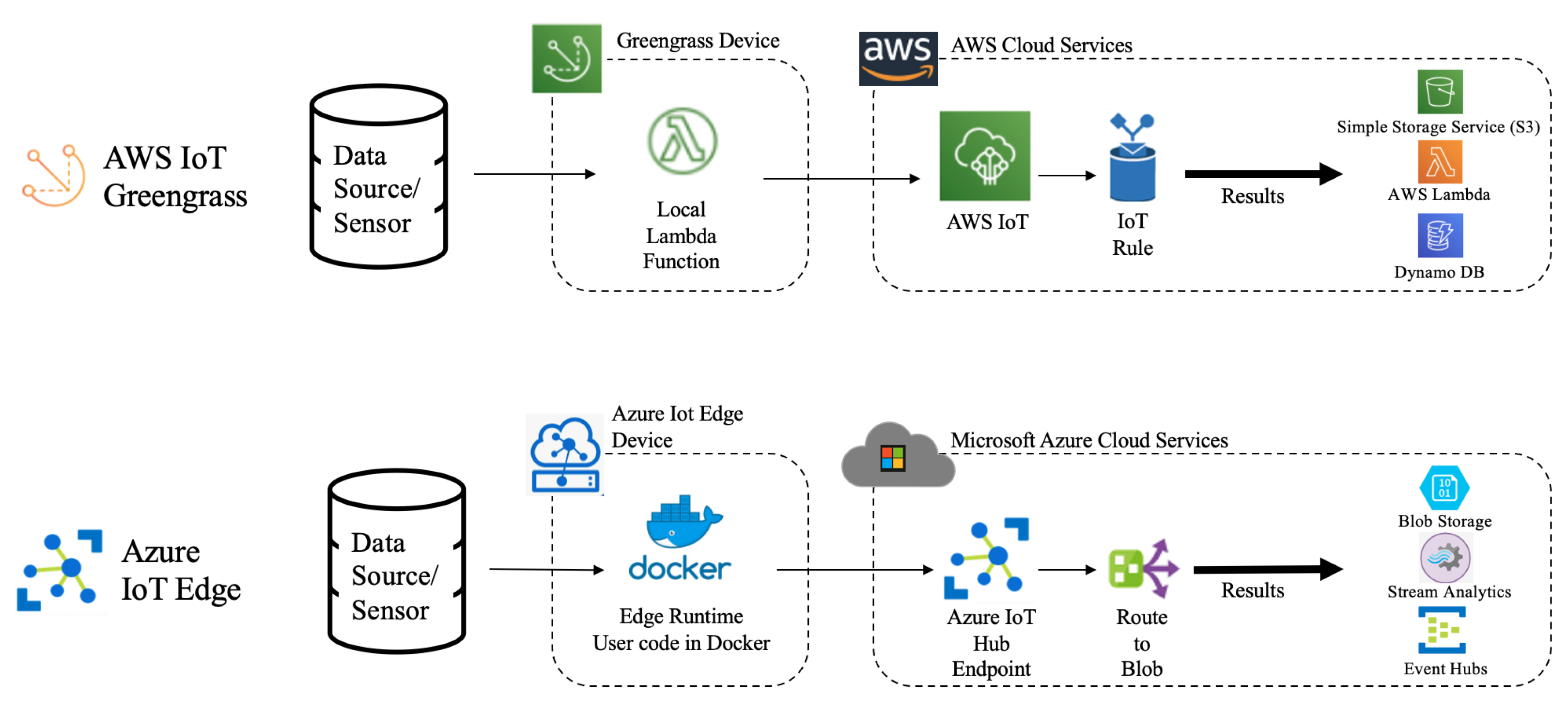
3.2. The EdgeBench Benchmark

In 2018, Das et al. [5] developed EdgeBench. This benchmark compares two serverless EC platforms from two different cloud providers: AWS IoT Greengrass from Amazon Web Services (AWS) and Azure IoT Edge from Microsoft. Figure 1 displays the environment setup, where each application processes a bank of input data on an edge device and sends the results to cloud storage. A lambda function processes the files in an edge device (in the AWS setup) and are then stored, and the processed results sent back to the user.

Figure 1. EdgeBench environmental setup.

This study first used three applications to quantify the differences between these platforms: one that transformed audio into text, another that performed image recognition, and an application that generated simulated temperature values. Later, we added three other applications to the benchmark: face-detection, matrix-reduction, and image-resizing applications. They used a Raspberry Pi model 3B as the edge device to perform the various tests. The benchmark consists of sending files from the edge device to the cloud, where they are processed and stored. Figure 2 displays the benchmark pipeline where the dataset has the files, and the user develops the code to upload such files from the edge device to the cloud for processing and storage. In our implementation, we also used an only-edge environment. Similar to the original authors, we also considered cloud-based implementation, where we analyzed the differences between an edge and edge-cloud (which we call cloud) environment. Through these implementations, we aim to check if processing files on the edge, with limited resources but less latency, is better than using the resourceful cloud services to process data with the drawback of higher latency values.

Figure 2. Benchmark pipeline.

Figure 3 presents the AWS example of the evaluated metrics:

Figure 3. EdgeBench metrics (AWS example).

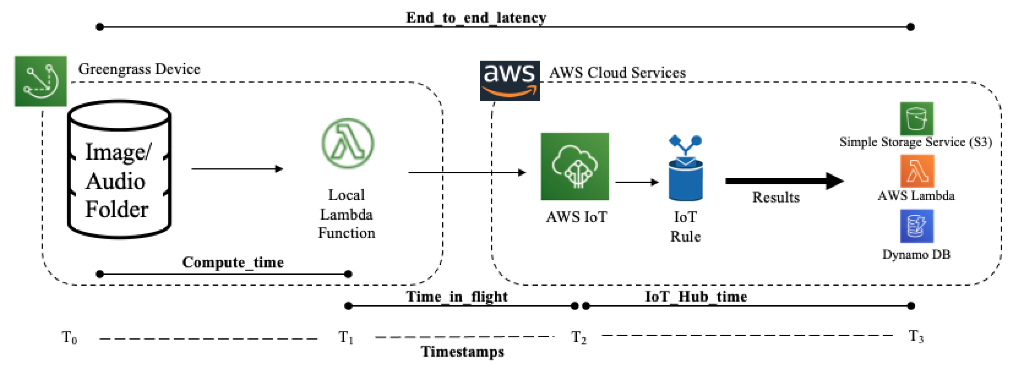
• “Time_in_flight” is the time spent sending data from the Raspberry Pi to the cloud ($T_2-T_1$).
• “IoT_Hub_time” is the time spent by the cloud storing the results of the computation of each task in an application’s workload ($T_3-T_2$).
• “Compute_time” corresponds to the time spent computing each task in question ($T_1-T_0$).
• “End_to_end_latency” is the total time spent solving the proposed problem, i.e., the sum of all times (sending, computing, and storing the result) ($T_3-T_0$).

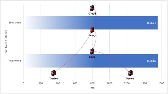
3.3. Real-World Environment

This section describes the setup of the real-world environment, which is located at the Centre for Informatics and Systems of the University of Coimbra (CISUC).

Due to the fact that the facilities had Wi-Fi issues leading to an unstable signal, we connected Raspberry Pi to a network point to achieve top speed. Raspberry Pi 3B has an Ethernet port with 10/100 Mbps bandwidth, and the obtained values were around 80 Mbps on average. The connection between the router and the internet service provider is around 1 Gbps.

Given the fundamental purpose of this paper, instead of applying the benchmark to two clouds, we opted for just one. We chose the Ireland AWS servers because these had lower latency between 55 and 60 ms. We also used the scripts at [20] offered by the authors of [5].

Lastly, we used the original datasets of [5] to send the scalar, audio, and image files.

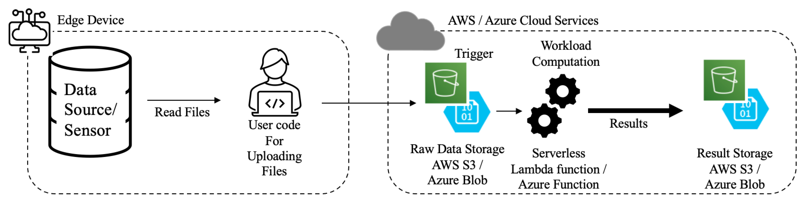
3.4. Simulation Environment

In this article, we only focus on implementing EdgeBench in FogComputingSim and references to the architecture and its explanation are in [3]. Therefore, this section only describes the various stages of the simulation environment on the basis of information provided in [5]. We installed the simulation tool on a MacBook Air computer with a dual-core i5 @1.6 GHz, with 16 GB of RAM (2133 MHz LPDDR3).

In [5], the authors set up three devices: a 3B Raspberry Pi used in this benchmark for computation performed at the edge, a proxy server that connects users to the Internet, and a device representing the services provided by the cloud, including one for processing and storage. Because the simulator only had a single object type, we differentiate these objects through their capabilities, defined by three primary parameters in their configuration, which are computation capacity in Millions of Instructions per Second (MIPS), the amount of RAM, and the storage in MB. Table 1 shows our device configuration. Regarding MIPS values, for the cloud, we used the average MIPS of an Intel Core i7-3960X (quad-core) @3.3 GHz. For Raspberry Pi model 3B, we used the average value of the ARM Cortex-A53 (quad-core) @1.2 GHz.

Table 1. Device configuration.

Device	CPU (MIPS)	RAM (MB)	Storage (MB)
Cloud	180,000	64	12,288
Proxy server	100	100	0
Raspberry Pi	10,000	1024	4096

Despite Vieira [3] stating that “both latency and bandwidth values for mobile communications are constant in the whole 2D plane”, we added noise to the simulation by setting a random value for both latency and bandwidth. We set these random values according to the works of [21,22]. Charyyev et al. [21] studied different cloud providers around the world and performed large-scale latency measurements from 8456 end users to 6341 edge servers and 69 cloud locations. From the authors’ results, we used the registered latency from 40% and 60% of the users. Accordingly, we set the minimal and maximal latency values for the edge simulations to be 5 and 10 ms respectively, and for the cloud simulations to be 10 and 20 ms. Regarding the bandwidth values, we also used a random number between 150 and 200 Mbps according to the tests performed in [22] and the type of network connection that CISUC research centre has.

In our simulation process, we ran each EdgeBench application dataset for 30 times (scalar, image, and audio) in both environments (edge and cloud). Figure 4 shows the average values of the edge and cloud latency for upload (Up) and download (Down) in ms, and the bandwidth upload (Up) and download (Down) in Mbps. These results correspond to the average of the 90 runs for each environment ($30runs\times 3datasets$).

Figure 4. Average values for simulated latency (ms) and bandwidth (Mbps).

We configured the Raspberry Pi device on the basis of data provided by the benchmark [5]. We assigned minimal values to the proxy server in terms of computational capacity because the goal was to compare the performance between Raspberry Pi and cloud. Lastly, the cloud is represented by an object with more computational resources than those of the others. We considered the Raspberry Pi’s real capabilities when adjusting the parameters in the simulator.

To represent the EdgeBench applications, namely, a temperature sensor, audio-to-text converter, and object recognition in images, we used three modules, according to programming model distributed data flow (DDF) [23]. The client module was hosted on the Raspberry Pi object and each application is assigned to a module responsible for data stream processing (scalars, audios, or images). Both the Raspberry Pi and the cloud can host each processing module. Finally, a cloud module stores the processed data. Figure 5 shows the DDF of the three EdgeBench applications.

Figure 5. Distributed data flow of applications.

Table 2 shows the workloads and their data dependencies between modules, considering the processing cost and the amount of transferred data. These values represent the simulation of the computation flow of each application.

Table 2. Data dependency between modules.

Dataset	Dependencies	Processing Cost (MIPS)	Data Size (Bytes)
Audio	Raw Data	2650	84,852
	Processed Data	5200	162
Image	Raw Data	800	131,707
	Processed Data	5300	750
Scalar	Raw Data	30	240
	Processed Data	5100	233

Since the workload was continuous throughout the simulation, the data size for each of the applications, pre- and post-processing, was obtained by averaging all data sent in each of the phases. Regarding computational load, as there was no available information that allowed for us to know the number of instructions executed per second for both the generation of data and their computation in each application, MIPS were the same in every simulation, although we used reference values of real-world CPUs.

4. Experimental Evaluation

This section presents the evaluation of FogComputingSim by analyzing the results from the simulator and those of the real-world environment using the same metrics.

4.1. Metrics

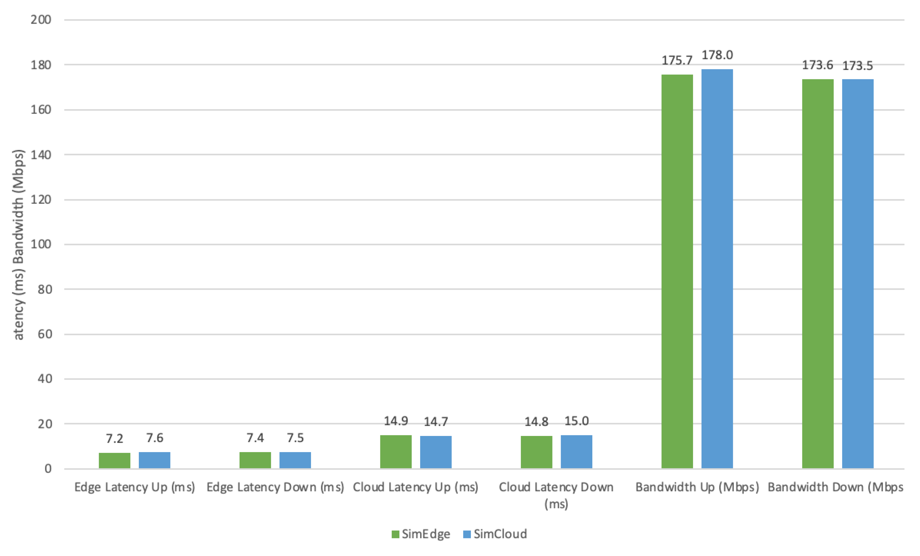
We evaluated the following metrics:

• Time_in_flight (ms)—time spent sending data from the Edge device (Raspberry Pi) to the cloud;
• IoT_Hub_time (ms)—time spent within the cloud to save the results;
• End_to_end_time (ms)—sum of the time “Time_in_flight” and “IoT_Hub_time”;
• Compute_time (ms)—time spent to compute the data;
• Payloadsize (bytes)—size of files uploaded to the cloud. If the computation is on the Raspberry Pi, it only sends the results file; if it is performed in the cloud, the full data file is sent;
• End_to_end_latency (ms)—total time spent, corresponds to the sum of the time: “End_to_end_time” and “Compute_time”.

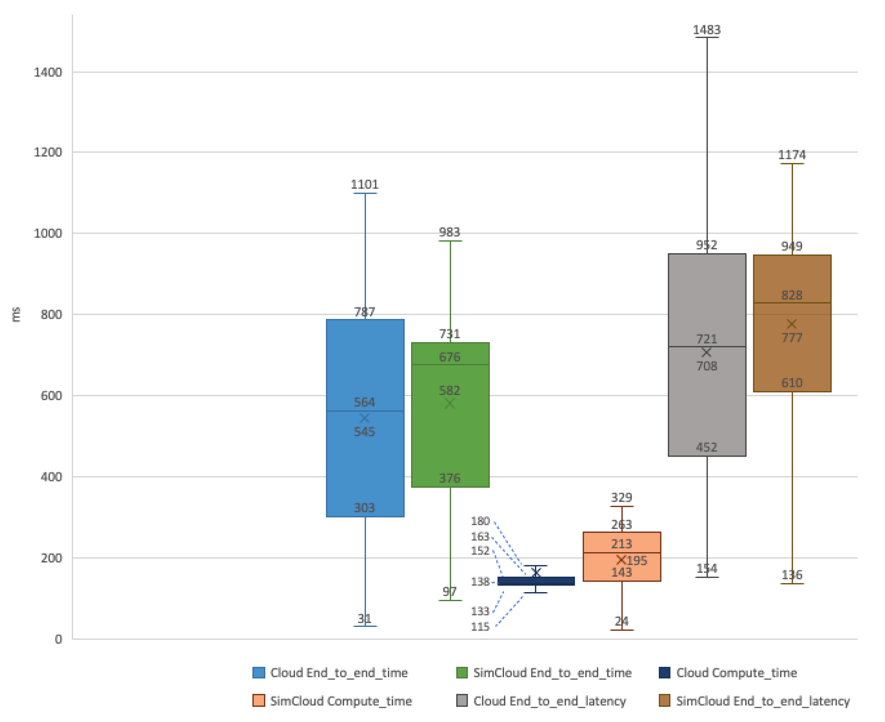
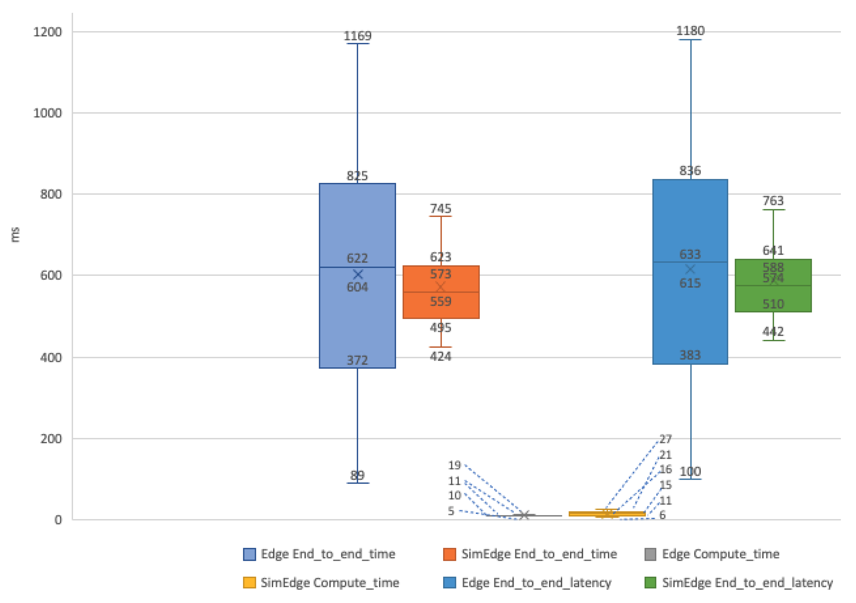
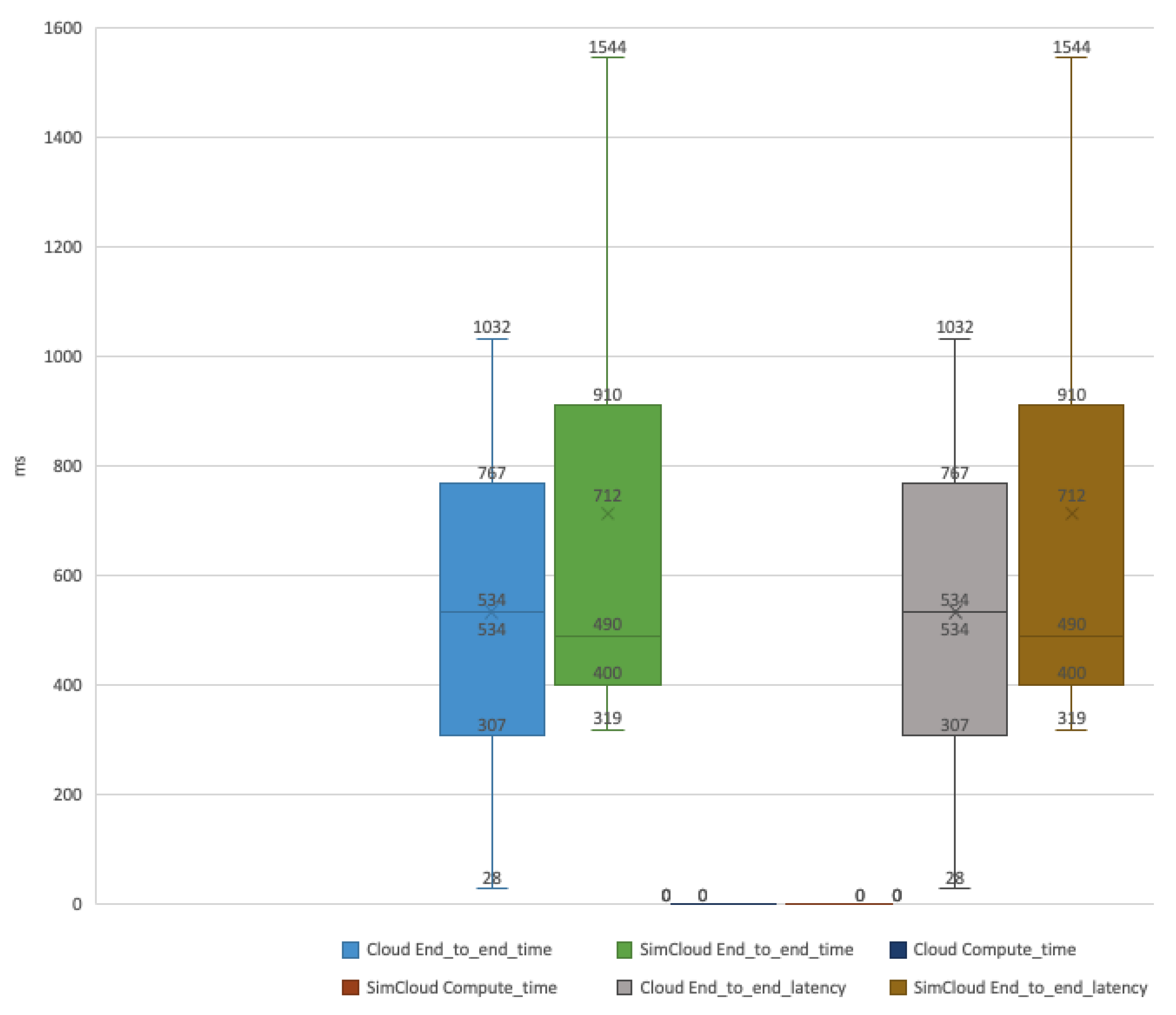
4.2. Benchmark Comparison

We evaluated FogComputingSim by comparing the real-world and simulated environment results from an average of 30 executions of each dataset in both environments. This assessment aimed to find if the results are reliable and realistic, to determine if this simulation tool is suitable to test new offloading techniques and help speed up the process of scientific development and innovation.

Table 3 provides the assessment of each application (scalar, image, and audio) in two environments: Edge (computing performed in Raspberry Pi 3B) and cloud (computing performed in the cloud). We identified the results with “Edge” and “Cloud”, and we represent the simulator results with the prefix “Sim”. Because of some network limitations at CISUC, we could not get the “Time_in_flight” and “IoT_Hub_time” metrics data for some cloud scenarios. However, it did not interfere with the “End_to_end_latency” time because the lack of data from these intermediate metrics did not alter the overall time spent in the data transfer and computation process. We configured each application’s modules regardless of the computation destination, at the Edge or in the cloud. The user is free to configure the simulator and edit the performance, processing, and connection values. The results show the simulator can perform accurate simulations with a setup similar to the benchmark execution.

Table 3. Evaluation results of EdgeBench in both environments.

Benchmark	Environment	Time_in_Flight (ms)	IoT_Hub _Time (ms)	End_to_ end_Time (ms)	Compute_ Time (ms)	End_to_ end_Latency (ms)	Payload Size (Bytes)
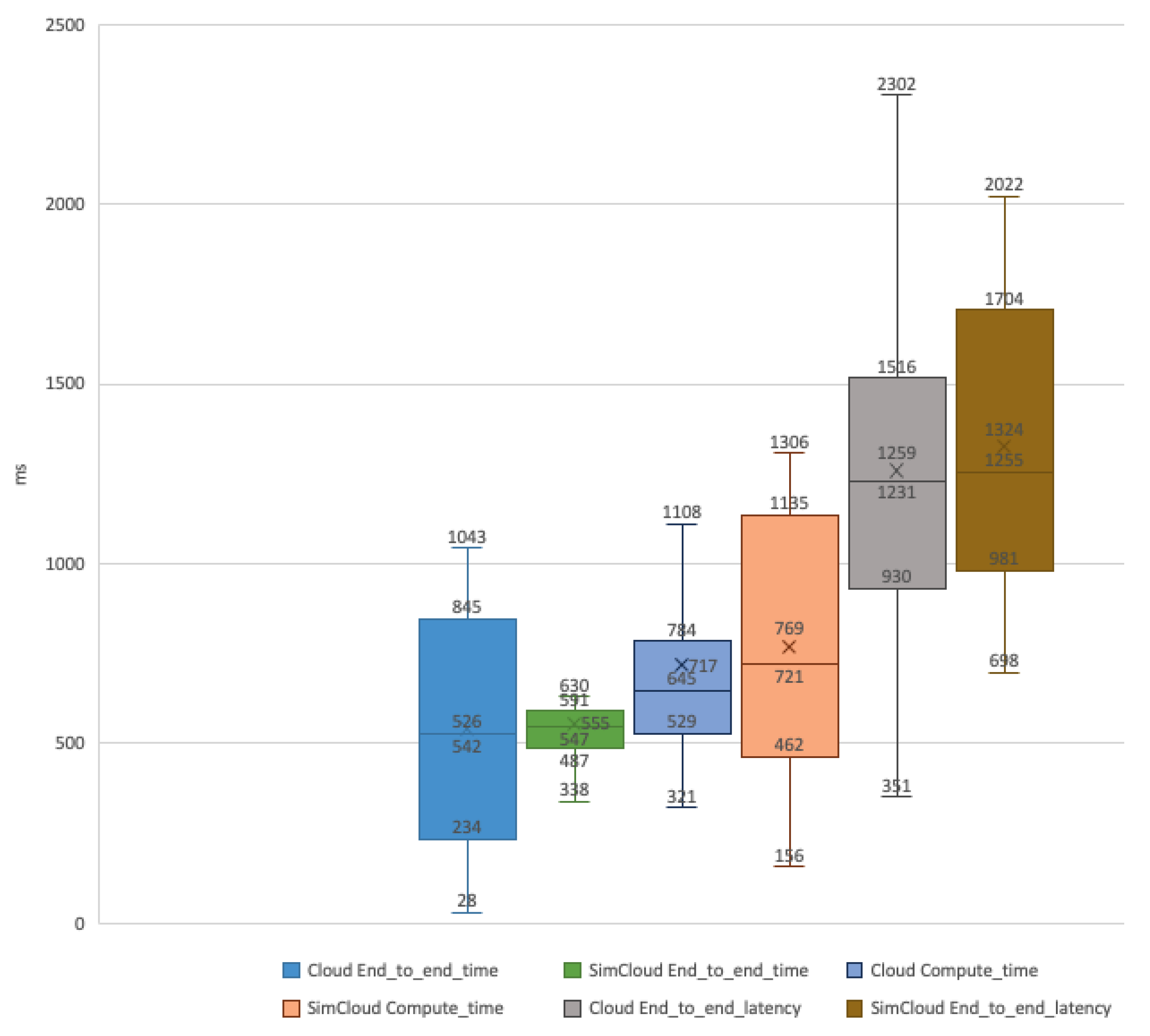
Scalar	Edge	34.82	569.05	603.87	10.92	614.78	234.00
	SimEdge	32.27	540.27	572.53	15.69	588.22
	Cloud	0.00	0.00	533.55	0.00	533.55	238.99
	SimCloud	32.63	679.48	475.64	0.00	475.64
Images	Edge	34.52	610.11	644.64	242.72	887.35	751.35
	SimEdge	35.27	574.68	609.95	280.34	890.29
	Cloud	0.00	0.00	544.97	162.66	707.63	131,707.42
	SimCloud	33.93	547.75	581.69	195.05	776.74
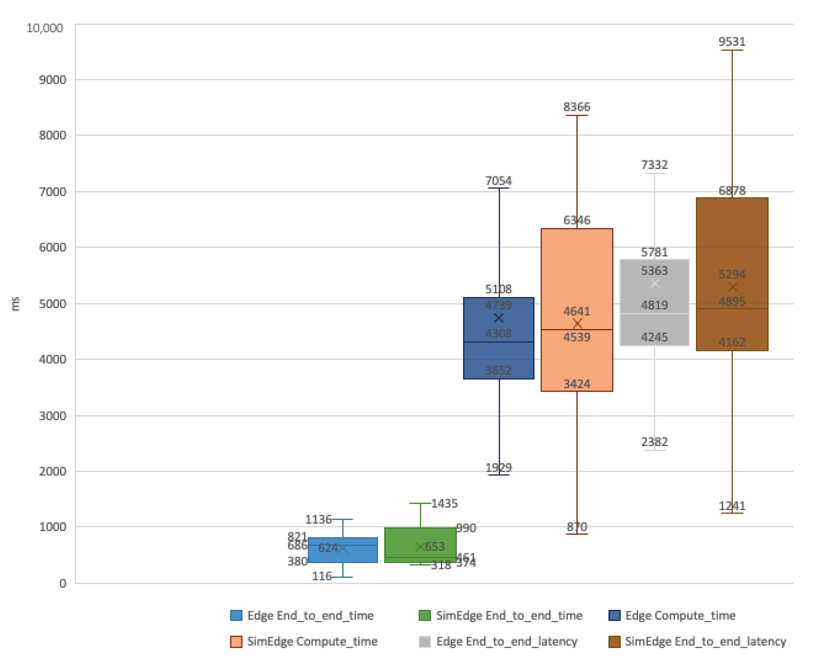
Audio	Edge	35.94	588.11	624.04	4739.11	5363.15	162.07
	SimEdge	26.23	626.91	653.14	4640.72	5293.86
	Cloud	0.00	0.00	542.05	716.63	1258.68	84,853.85
	SimCloud	31.30	523.74	555.04	769.02	1324.06

In the analysis, for visualization purposes, Figure 6, Figure 7, Figure 8, Figure 9, Figure 10 and Figure 11 display only 3 metrics (End_to_end_time, Compute_time, and End_to_end_latency) for both environments: real world (Edge/Cloud) and simulated (SimEdge/SimCloud). The box plot provides the following values: minimum, quartile 25%, median, quartile 50%, average (x mark), quartile 75%, and maximum. We removed the outlier points from the figures but not from the assessment, and used an inclusive median in the quartile calculation.

Figure 6. Scalar application in the edge (time in ms).

Figure 7. Scalar application in the cloud (time in ms).

Figure 8. Image application in the edge (time in ms).

Figure 9. Image application in the cloud (time in ms).

Figure 10. Audio application in the edge (time in ms).

Figure 11. Audio application in the cloud (time in ms).

In Figure 6, for the edge scenario, the simulator generated more stable results than those registered in the real-world environment, mainly due to low processing and network requirements for this dataset in this environment. The fluctuation of values in “IoT_Hub_time”, represented in the “End_to_end_time”, in the real-world environment contributed to the overall difference, without influencing the average difference between environments that is only around 25ms. Concerning the cloud (Figure 7), it is possible to visualize that the time spent in the computation of the scalar data (Compute_time) is almost zero in both environments. The second difference relates to the total time spent (End_to_end_latency), which is higher in the real-world environment than the time spent in the simulator, regarding the average value. However, the real-world scenario had a lower fluctuation amongst registered values, but a higher overall average (around 60 ms).

In Figure 8 the differences in the “End_to_end_time” (higher in the real-world environment) and “Compute_time” (higher in the simulation), lead to similar overall average time, with the simulated environment taking more 3ms in average to execute the dataset. In Figure 9, also “End_to_end_time” and “Compute_time” the simulation took more time, resulting in an “End_to_end_latency” around 70 ms higher.

Figure 10 display the results for the audio application. In the simulated edge environment, there was a higher fluctuation of values concerning computation time (Compute_ time) and final latency, but presenting an overall average value of “End_to_end_latency” around 70 ms less than the real-world implementation. In Figure 11, the real-world environment had a greater amplitude of values for “End_to_end_time”, while the simulated scenario had a higher amplitude of values in “Compute_time”, which represents an overall higher amplitude for “End_to_end_latency” in the real-world environment but also around 80 ms less than the simulation.

Table 4 displays the “End_to_end_latency” statistics. In the experiments using the scalar dataset, both simulated scenarios performed better than the real world with 4.3% and 10.9%, respectively. Using the Image dataset, the real-world implementation was faster by 0.3% and 9.8% in the edge and cloud scenarios, respectively. Lastly, in the experiments using the Audio dataset, the real world was slower (1.3%) in the edge and faster (5.2%) in the cloud. Overall, the simulated environment was faster 0.2% than the real world, which allows us to state that the configurations that we deployed can simulate a real environment.

Table 4. End_to_end_latency statistical results of the EdgeBench in both environments.

Benchmark	Environment	End_to_end_Latency (ms)
		Minimum	Quartile 25%	Median	Quartile 75%	Maximum	Average	Std. Dev.
Scalar	Edge	99.57	383.89	630.23	833.07	1179.98	614.78	277.78
	SimEdge	442.27	510.21	574.10	640.69	1083.18	588.22	123.51
	Cloud	28.33	307.46	533.75	767.12	1032.22	533.55	286.72
	SimCloud	201.95	251.13	321.65	622.05	1054.56	475.64	274.95
Images	Edge	293.92	598.59	878.80	1112.32	7583.10	887.35	548.48
	SimEdge	474.62	558.39	627.11	1370.62	1830.72	890.29	469.38
	Cloud	153.73	451.90	720.86	951.60	3327.76	707.63	332.92
	SimCloud	136.30	609.89	828.40	948.67	1174.24	776.74	239.76
Audio	Edge	2382.31	4245.45	4819.48	5780.76	19426.96	5363.15	2530.41
	SimEdge	1240.63	4162.39	4895.30	6877.90	9530.80	5293.86	2051.92
	Cloud	350.95	930.48	1230.97	1515.55	3126.76	1258.68	489.23
	SimCloud	698.44	981.00	1255.43	1704.40	2021.79	1324.06	407.09

4.3. Work Limitations

We acknowledge some limitations to our work, and we mention the ones that we consider relevant:

• Despite our changes in FogComputingSim to allow for some network fluctuations, this simulator is not a network simulator and thereby ignores network effects at the cost of minor differences in data transmission. Network effects are a motivation for offloading in the first place, and it is a limitation that we considered in assessing the results.
• The use of a single benchmark and setup limits the conclusions that can be taken from the overall simulator validity. While it can give some clear indications, further tests and setups are needed to obtain a more clear assessment.

5. Conclusions and Future Work

The evaluation of EC simulator FogComputingSim aimed to understand if the results obtained from this simulator were consistent with those achieved in real-world environments. Although there are some works on simulation environments in EC, there awerere no validations of the gathered results. This work is significant because we implemented and compared the EdgeBench benchmark in the real world and a simulated environment to analyze the simulator’s capabilities. Due to the fact that the experimental results were similar in most of the analyzed metrics, we could conclude that the FogComputingSim enables a valid first approach to the study of EC scenarios. Then, we can trust EC simulations, if the right simulator configurations are setup, to achieve reliable and representative results, notwithstanding the specific simulator limitations. Our aim was to see if we could achieve real-world values in a simulated environment. With the deployed configurations, we were able to reach this goal. Therefore, we could now use it in other scenarios knowing that the results would be identical to those of real-world implementations. Nevertheless, in a final development phase, the obtained results do not fully replace real-world implementation.

As future work, we intend to study additional applications and benchmarks, test different setups and topologies, and extend our study to include other simulators.

References

- Carvalho, G.; Cabral, B.; Pereira, V.; Bernardino, J. Computation offloading in Edge Computing environments using Artificial Intelligence techniques. Eng. Appl. Artif. Intell. 2020, 95, 103840. [Google Scholar] [CrossRef]
- Shakarami, A.; Ghobaei-Arani, M.; Shahidinejad, A. A survey on the computation offloading approaches in mobile edge computing: A machine learning-based perspective. Comput. Netw. 2020, 182, 107496. [Google Scholar] [CrossRef]
- Vieira, J.C. Fog and Cloud Computing Optimization in Mobile IoT Environments. Ph.D. Thesis, Instituto Técnico de Lisboa, Lisbon, Portugal, 2019. [Google Scholar]
- Gupta, H.; Dastjerdi, A.V.; Ghosh, S.K.; Buyya, R. iFogSim: A Toolkit for Modeling and Simulation of Resource Management Techniques in Internet of Things, Edge and Fog Computing Environments. Softw. Pract. Exp. 2017, 47, 1275–1296. [Google Scholar] [CrossRef] [Green Version]
- Das, A.; Patterson, S.; Wittie, M. Edgebench: Benchmarking edge computing platforms. In Proceedings of the 2018 IEEE/ACM International Conference on Utility and Cloud Computing Companion (UCC Companion), Zurich, Switzerland, 17–20 December 2018; pp. 175–180. [Google Scholar]
- Mahmud, R.; Buyya, R. Modeling and Simulation of Fog and Edge Computing Environments Using iFogSim Toolkit. In Fog and Edge Computing: Principles and Paradigms, 1st ed.; Srirama, R.B.S.N., Ed.; Wiley: Hoboken, NJ, USA, 2019; Chapter 17; pp. 433–464. [Google Scholar]
- Awaisi, K.S.; Assad, A.; Samee, U.K.; Rajkumar, B. Simulating Fog Computing Applications using iFogSim Toolkit. In Mobile Edge Computing; Springer: Berlin/Heidelberg, Germany, 2021; pp. 5–22. [Google Scholar] [CrossRef]
- Skarlat, O.; Nardelli, M.; Schulte, S.; Borkowski, M.; Leitner, P. Optimized IoT service placement in the fog. Serv. Oriented Comput. Appl. 2017, 11, 427–443. [Google Scholar] [CrossRef]
- Duan, K.; Fong, S.; Zhuang, Y.; Song, W. Carbon Oxides Gases for Occupancy Counting and Emergency Control in Fog Environment. Symmetry 2018, 10, 66. [Google Scholar] [CrossRef] [Green Version]
- Mahmoud, M.M.E.; Rodrigues, J.J.P.C.; Saleem, K.; Al-Muhtadi, J.; Kumar, N.; Korotaev, V. Towards energy-aware fog-enabled cloud of things for healthcare. Comput. Electr. Eng. 2018, 67, 58–69. [Google Scholar] [CrossRef]
- Mutlag, A.A.; Khanapi Abd Ghani, M.; Mohammed, M.A.; Maashi, M.S.; Mohd, O.; Mostafa, S.A.; Abdulkareem, K.H.; Marques, G.; de la Torre Díez, I. MAFC: Multi-Agent Fog Computing Model for Healthcare Critical Tasks Management. Sensors 2020, 20, 1853. [Google Scholar] [CrossRef] [Green Version]
- Kumar, H.A.; J, R.; Shetty, R.; Roy, S.; Sitaram, D. Comparison Of IoT Architectures Using A Smart City Benchmark. Procedia Comput. Sci. 2020, 171, 1507–1516. [Google Scholar] [CrossRef]
- Jamil, B.; Shojafar, M.; Ahmed, I.; Ullah, A.; Munir, K.; Ijaz, H. A job scheduling algorithm for delay and performance optimization in fog computing. Concurr. Comput. Pract. Exp. 2020, 32, e5581. [Google Scholar] [CrossRef]
- Bala, M.I.; Chishti, M.A. Offloading in Cloud and Fog Hybrid Infrastructure Using iFogSim. In Proceedings of the 2020 10th International Conference on Cloud Computing, Data Science Engineering (Confluence), Noida, India, 29–31 January 2020; pp. 421–426. [Google Scholar] [CrossRef]
- Naouri, A.; Wu, H.; Nouri, N.A.; Dhelim, S.; Ning, H. A Novel Framework for Mobile-Edge Computing by Optimizing Task Offloading. IEEE Internet Things J. 2021, 8, 13065–13076. [Google Scholar] [CrossRef]
- Wang, C.; Li, R.; Li, W.; Qiu, C.; Wang, X. SimEdgeIntel: A open-source simulation platform for resource management in edge intelligence. J. Syst. Archit. 2021, 115, 102016. [Google Scholar] [CrossRef]
- Varghese, B.; Wang, N.; Bermbach, D.; Hong, C.H.; de Lara, E.; Shi, W.; Stewart, C. A Survey on Edge Benchmarking. arXiv 2020, arXiv:2004.11725. [Google Scholar]
- Yang, Q.; Jin, R.; Gandhi, N.; Ge, X.; Khouzani, H.A.; Zhao, M. EdgeBench: A Workflow-based Benchmark for Edge Computing. arXiv 2020, arXiv:2010.14027. [Google Scholar]
- Halawa, H.; Abdelhafez, H.A.; Ahmed, M.O.; Pattabiraman, K.; Ripeanu, M. MIRAGE: Machine Learning-based Modeling of Identical Replicas of the Jetson AGX Embedded Platform. In Proceedings of the 2021 IEEE/ACM Symposium on Edge Computing (SEC), San Jose, CA, USA, 14–17 December 2021; pp. 26–40. [Google Scholar]
- Das, A.; Park, T.J. GitHub—rpi-nsl/Edgebench: Benchmark for Edge Computing Platforms. 2019. Available online: https://github.com/rpi-nsl/edgebench (accessed on 1 April 2022).
- Charyyev, B.; Arslan, E.; Gunes, M.H. Latency Comparison of Cloud Datacenters and Edge Servers. In Proceedings of the GLOBECOM 2020—2020 IEEE Global Communications Conference, Taipei, Taiwan, 7–11 December 2020; pp. 1–6. [Google Scholar] [CrossRef]
- Sackl, A.; Casas, P.; Schatz, R.; Janowski, L.; Irmer, R. Quantifying the impact of network bandwidth fluctuations and outages on Web QoE. In Proceedings of the 2015 Seventh International Workshop on Quality of Multimedia Experience (QoMEX), Pilos, Greece, 26–29 May 2015; pp. 1–6. [Google Scholar] [CrossRef]
- Giang, N.K.; Blackstock, M.; Lea, R.; Leung, V.C.M. Distributed Data Flow: A Programming Model for the Crowdsourced Internet of Things. In Proceedings of the Doctoral Symposium of the 16th International Middleware Conference, Vancouver, BC, Canada, 7–11 December 2015; Association for Computing Machinery: New York, NY, USA, 2015. [Google Scholar]