Improved Bidirectional GAN-Based Approach for Network Intrusion Detection Using One-Class Classifier

Abstract

Existing generative adversarial networks (GANs), primarily used for creating fake image samples from natural images, demand a strong dependence (i.e., the training strategy of the generators and the discriminators require to be in sync) for the generators to produce as realistic fake samples that can “fool” the discriminators. We argue that this strong dependency required for GAN training on images does not necessarily work for GAN models for network intrusion detection tasks. This is because the network intrusion inputs have a simpler feature structure such as relatively low-dimension, discrete feature values, and smaller input size compared to the existing GAN-based anomaly detection tasks proposed on images. To address this issue, we propose a new Bidirectional GAN (Bi-GAN) model that is better equipped for network intrusion detection with reduced overheads involved in excessive training. In our proposed method, the training iteration of the generator (and accordingly the encoder) is increased separate from the training of the discriminator until it satisfies the condition associated with the cross-entropy loss. Our empirical results show that this proposed training strategy greatly improves the performance of both the generator and the discriminator even in the presence of imbalanced classes. In addition, our model offers a new construct of a one-class classifier using the trained encoder–discriminator. The one-class classifier detects anomalous network traffic based on binary classification results instead of calculating expensive and complex anomaly scores (or thresholds). Our experimental result illustrates that our proposed method is highly effective to be used in network intrusion detection tasks and outperforms other similar generative methods on two datasets: NSL-KDD and CIC-DDoS2019 datasets.

1. Introduction

Network intrusion detection is used to discover any unauthorized attempts to a network by analyzing network traffic coming in and out of the network and looking for any signs of malicious activity. This is often regarded as one of the most critical network security mechanisms to block or stop cyberattacks [1].

Traditional machine learning (ML) approaches, such as supervised network intrusion detection, have shown reasonable performance for detecting malicious payloads included in network traffic-based data sets labeled with ground truth [2]. However, with the mass increase in the size of data, it has become either too expensive or no longer possible to label a huge number of data sets (i.e., big data) [3]. Unsupervised intrusion detection methods have been proposed as it no longer demands the requirement for labeled data. In addition, these unsupervised methods can utilize only the samples from one class (e.g., normal samples) for training to recognize any patterns that deviate from the training observations. However, the detection accuracy of these unsupervised learning methods tends to suffer as soon as an imbalanced class appears (e.g., the number of samples in a class is significantly more or less compared to the number of samples in other classes).

A number of generative models have been proposed including Autoencoders [4] and generative adversarial networks (GANs) [5] with the ability to generate realistic synthetic data sets to improve detection accuracy based on anomaly detection techniques.

Autoencoder (AE) is composed of an encoder and decoder. The encoder can compress high-dimensional input data into low-dimensional latent space. The decoder generates the output that resembles the input by reassembling the (reduced) data representation from the latent space. Typically, a reconstruction loss is computed between the output and the input and used as a mechanism to identify anomalies. The encoder in AE captures the semantic attributes of the input data into the latent space, as a form of vector representation, to represent the corresponding input sample from the real data space.

In particular, GANs have emerged as a leading yet very powerful technique for generating realistic data sets, especially in the image identification and processing involved in the natural images despite arbitrarily complex data distributions that exist in the real data sets. In GANs, two deep neural networks, the generator and the discriminator, respectively, are involved in the main GANs’ structure. The generator and the discriminator are trained in turn by playing an adversarial game. That is, the generator produces the output (i.e., somewhat based on the distribution of real data) while the discriminator takes the fake data (i.e., the output of the generator) and real data as input and aims to distinguish them. The goal of the generator is to generate the fake data that resembles as much as the real data to “fool” the discriminator (i.e., it can’t distinguish the fake data from real data). The generator and the discriminator are highly dependent on each other to reach the optima.

Rather than only generating synthetic images that resemble the original input, anomaly detection-based GAN approaches have been proposed to classify abnormal images whose feature deviates significantly from the original images [6,7,8]. Moving from applying anomaly detection-based GAN on images, several works such as [9,10] attempted to apply the same principle for network intrusion detection tasks.

However, there are two issues with these existing methods. The first issue is the strong dependence between the generator and the discriminator. That is, the number of training iterations both the generator and the discriminator go through are typically in sync. However, this dependence can be relaxed for the network intrusion tasks because of the difference in the input structure that is fed to GAN models. For network intrusion inputs, the dimensionality of features is significantly lower compared to images, the majority of features in the network intrusion datasets are discrete, as well as the size of inputs relatively smaller. Due to these reasons, the training of the discriminator does not require as many iterations to assess the difference between the synthetic data and the real input [10]. The second issue is the complexity of producing anomaly scores that are used to decide which input samples are normal or not. The existing methods used on images typically use at least two or more loss functions to accurately produce anomaly scores. However, text-based network intrusion inputs whose structure is a lot simpler than images, a simpler loss function can be used.

To address these two issues, we propose a new Bidirectional GAN (Bi-GAN) model that can effectively detect network intrusions without unnecessary training steps and with a simpler loss function.

The contributions of our proposed approach are following:

• We relax the requirement for the generator and the discriminator to train them in sync. The generator (along with the encoder) in our proposed model goes through more rigorous training iterations in order to produce more reliable synthetic data set that highly resembles the real traffic samples. This can effectively remove any overheads associated with the discriminator trained overly. Our proposed model shows that the generator’s performance is greatly improved by offering the generator (and encoder) to train more than the discriminator, which in turn, also actually improves the discriminator’s performance better.
• In our promised model, a cross-entropy is used to keep track of the overall balance in terms of the number of relative training iterations required for the generator and the discriminator. In addition, we employ a -log (D) trick to train the generator to obtain sufficient gradient in the early training stage by inverting the label.
• We offer new construction of a one-class classifier using the trained encoder-discriminator for detecting anomalous traffic from normal traffic instead of having to calculate either anomaly scores or thresholds which are computationally expensive and complex.
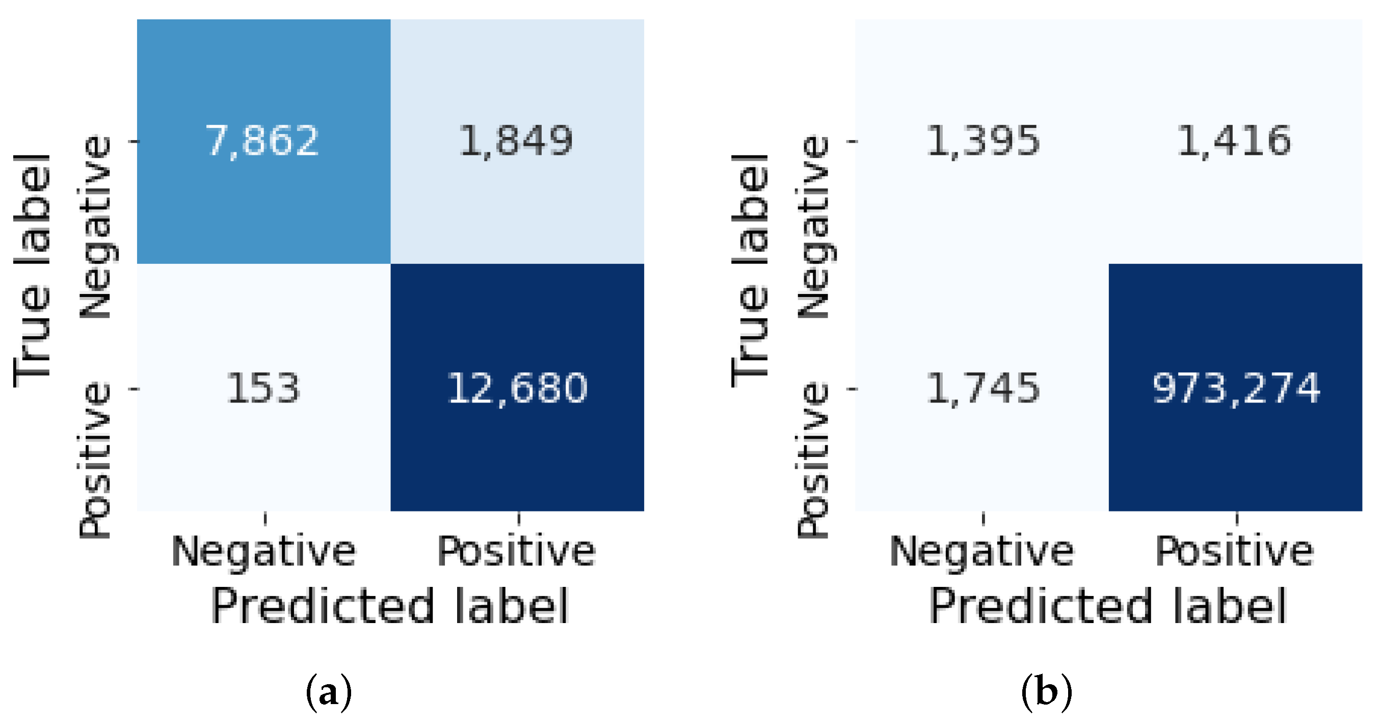
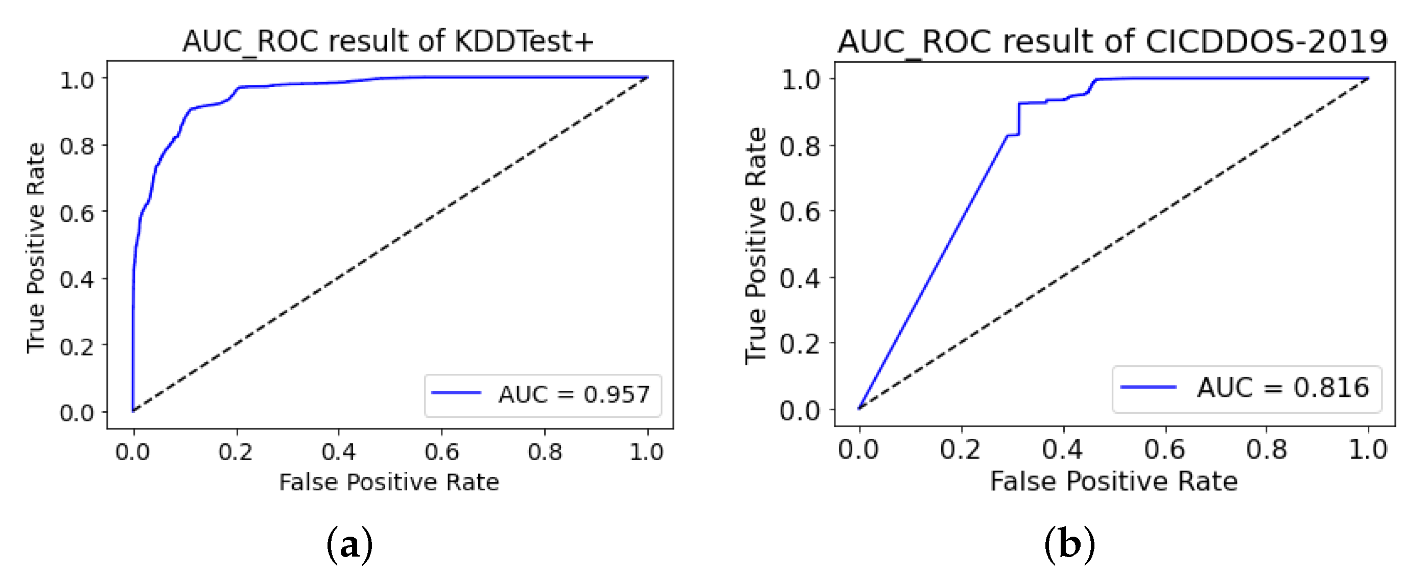
• Our experimental result shows that our proposed method is highly effective in using a GAN-based model for network anomaly detection tasks by achieving more than 92% F1-score on the NSL-KDD dataset and more than 99% F1-score on the CIC-DDoS2019 dataset.

The rest of this paper is organized as follows. Section 2 summarizes the review of the literature relevant to our study. Background knowledge in the generic GAN and BiGAN that is required to understand our study is presented in Section 3. Section 4 describes the details of our proposed model. Section 5 describes the data and the data preprocessing methodologies we used while Section 6 demonstrates our experimental results and provides analysis. Section 7 provides the concluding remarks along with the future work that is planned.

2. Related Work

In this section, we review the existing state-of-arts that use two generative deep learning models, Autoencoder and GAN, to detect anomalies (i.e., including intrusions) using anomaly-based detection approaches.

The autoencoder-based approaches typically use reconstruction methods where computing a reconstruction error and use it as a threshold to detect anomalies [11,12,13,14]. In this approach, an autoencoder is trained only with the normal samples to learn the distribution in their latent representation and use the distribution to reconstruct the input. The difference in the input and output termed reconstruction error is used to detect anomalies that typically generate high reconstruction loss compared to the normal samples. The work suggested by [15] confirmed the efficiency of such an anomaly-based autoencoder approach to be useful by showing a higher accuracy in network intrusion detection compared to existing (shallow) machine learning techniques. Other improved versions of the autoencoder approach were suggested to improve network intrusion detection. In [16], the authors used a Denoising Autoencoder (DAE) to remove the features that potentially degrade the overall performance, termed as noises, using stochastic analysis. An and Cho (2015) [12] proposed a Variational Autoencoder (VAE) based approach which used Gaussian distribution of input samples and use them as a part of reconstruction loss to identify anomalies.

GAN-based models for anomaly detection tasks came later than Autoencoders mostly from the field of computer vision. Schlegl et al. proposed AnoGAN [6], which was the first anomaly detection-based model. They further proposed f-AnoGAN [7], which improved the computational efficiency by adding an encoder before the generator to enable the mapping from data to the latent space directly thus avoiding expensive extra backpropagation. GANomaly [8] further improves the performance which adds two encoders. In their approach, one encoder is used before the generator to learn the latent space of the original data while the other encoder is used after the generator to learn the latent space of the reconstructed data.

BiGAN further improved its ability to detect anomalies in a simpler way with the ability of mapping data to latent space more efficiently. The BiGAN also comprises three components similar to many previous GAN variants used in anomaly-based detection. These include the generator, the discriminator, and an encoder, but have a different structure. In BiGAN, the encoder is independent of the generator as another input source for the discriminator. In this way, the BiGAN can learn to map the latent space to data (by the generator) and vice versa (by the encoder) simultaneously.

Efficient GAN [17] utilized BiGAN’s ability of inverse learning and demonstrated that it can be effectively used to detect anomalies not only on images but also on network intrusion datasets such as using the KDD99 dataset. In their approach, they introduced two similar losses as f-AnoGAN to form the anomaly score function. Since the encoder and the generator can compose an auto-encoder structure, ref. [10] suggests adding an Autoencoder style training step to the original BiGAN architecture to stabilize the model.

In the existing GAN approaches, there is a strong dependence between the generator and the discriminator. That is, the training strategy for the generator and the discriminator needs to be in sync to produce synthetic data that resembles the original images. This is necessary for images where the inputs have high dimensions, feature values are complex, and input size is large. However, network intrusion inputs are simpler, with fewer dimensions, the majority of features are discrete features, and the input size is relatively small. In this case, the dependence of training between the generator and the discriminator can be relaxed [10].

In addition, many existing methods require at least two or even more loss metrics to compute anomaly scores which have proven to be very expensive [7,8,17]. However, it has been shown in [10,18], that a more straightforward resolution could be used such as using the discriminator as a one-class classifier to detect anomalies instead of computing anomaly scores.

3. Background

3.1. Generic GAN

In a generic GAN approach, two neural networks, namely the generator and the discriminator, respectively, contest with each other in a game approach—generally in the form of a zero-sum game where one agent’s gain is another agent’s loss. The generative network (i.e., the generator) generates new data samples from a low dimensional distribution while the discriminative network (i.e., the discriminator) evaluates them. In another word, the generator learns to map from random noise to a data distribution of the real data while the discriminator distinguishes the new datasets generated by the generator (i.e., regarded as fake data) from the true data distribution. Figure 1 illustrates the architecture of the GAN.

Figure 1. Structure of GAN. The generator G map the input z (i.e., random noise) in latent space to produce a high dimensional $G\left(z\right)$ (i.e., fake samples). The discriminator D is expected to separate x (i.e., real samples) from $G\left(z\right)$.

Algorithm 1 demonstrates the procedure involved in the training phase of a generic GAN model. The generator takes a batch of vectors z (e.g., randomly drawn from a Gaussian distribution) and maps to $G\left(z\right)$ which has the same dimensions as the real samples x. The discriminator receives two sources of input (i.e., fake samples and real samples) and tries to distinguish them. The loss between the observation and the prediction at the discriminator is calculated and subsequently used to update both the generator and the discriminator until the training is complete.

It must be noted that there is no independent loss function for the generator in the standard GAN as it is updated indirectly with the objective function linked to the discriminator. Equation (1) depicts the objective of $V(G,D)$ for measuring the residual and optimizing both the generator and the discriminator.

$$\underset{G}{min}\underset{D}{max}V(G,D)={\mathbb{E}}_{x\sim pX}[logD\left(x\right)]+{\mathbb{E}}_{z\sim pZ}[log(1-D\left(G\left(z\right)\right))]$$

(1)

Algorithm 1: Training in Generic GAN

3.2. Bidirectional GAN

Bidirectional GAN or BiGAN is a variant of GAN by adding an encoder to the original GAN model. With the added encoder, the BiGAN is capable to learn the inverse mapping from the real data to the latent space [19,20] to better support the generator producing more semantically rich synthetic datasets. The encoder here plays an importable role for the BiGAN model by providing the learning the latent representation from the real data [19]. Figure 2 illustrates the architecture of BiGAN, and Algorithm 2 depicts the training involved in the BiGAN approach.

Figure 2. Structure of BiGAN. Note that (z and $E\left(x\right)$) and ($G\left(z\right)$ and x) have the same dimensions. The concatenated pairs $\left[G\right(z),z]$ and $[x,E(x\left)\right]$ are the two input sources of the discriminator D. The Generator G and the encoder E are optimized with the loss generated by the discriminator D.

Like the standard GAN, the training is comprised of two steps. The first step involves training the discriminator (D) to maximize the objective function described in Equation (2) without updating the generator (G) or encoder (E). The second step involves training both the generator and encoder to minimize the same objective function linked to the discriminator (D).

$$\begin{array}{cc}\underset{G,E}{min}\underset{D}{max}L(D,E,G)\hfill & ={\mathbb{E}}_{x\sim pX}\left[{\mathbb{E}}_{z\sim pE(·|x)}\right[logD(x,z)\left]\right]\hfill \\ & +{\mathbb{E}}_{z\sim pZ}\left[{\mathbb{E}}_{x\sim pG(·|z)}[log(1-D(x,z))]\right]\hfill \end{array}$$

(2)

Though the generator (and accordingly encoder) and the discriminator are trained separately, there is only one single objective function computed by the discriminator D. Both the generator and the encoder are updated indirectly through discriminator. Different from the standard GAN approach, a concatenation operation is added in the discriminator. The concatenation is to link the data x (or $G\left(z\right)$) with its latent space $E\left(x\right)$ (or z) and these two concatenated data are then inputted into the discriminator. When optimized, the G and the E are the inverses mapping to each other [19,20] which can be shown as $x=G\left(E\right(x\left)\right)$ and $z=E\left(G\right(z\left)\right)$.

Algorithm 2: Training in BiGAN

4. Our Proposed Model

Extending from the BiGAN approach, our proposed model offers a new training strategy for the generator and encoder. By further relaxing the dependence with the discriminator, our proposed model allows the generator and encoder to train until they produce a set of new data samples that resembles the real distribution of the original data while maintaining strong semantic relationships that exist in the text-based features of the original network traffic samples. Our proposed model also offers a new construct for the trained encoder–discriminator to use as a one-class binary classifier.

4.1. Main Components

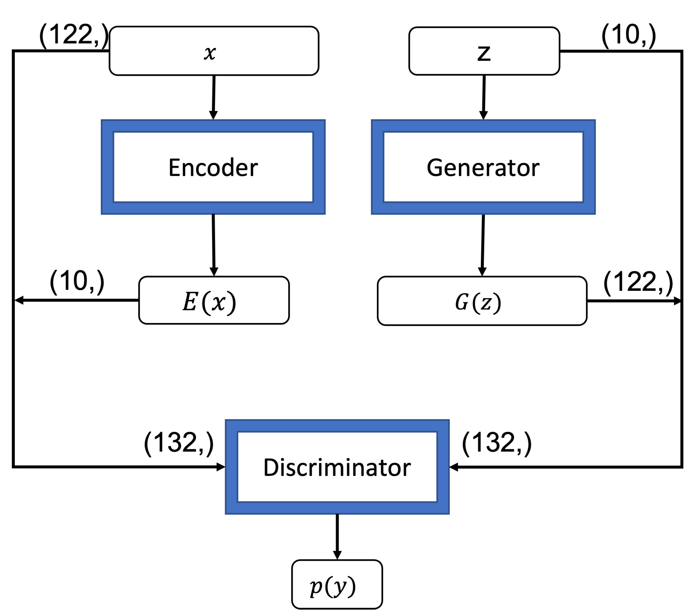
4.1.1. Encoder

The encoder in our proposed model is used for learning feature representation [20] which takes the real samples as inputs and maps them to a low dimensional vector in a latent space. In our approach, the encoder is a neural network with three dense layers and has ReLU as the activation function for the hidden layer and the output layer. As this typically works as an inverse mapping of the generator, the size of the latent space is typically set at the same dimension size of the input data used for the generator.

4.1.2. Generator

The generator in our approach maps a low-dimensional vector (i.e., random input values) to a higher-dimensional vector in the latent space. The generator acts exactly opposite to the encoder. It accepts a n-dimensional noise as the input source and the n is identical to the dimension size of latent space in the encoder. Our generator draws the n-dimensional noise from the standard normal distribution. The generator has a neural network structure of three dense layers. ReLU is used as the activation function for the hidden layer while the sigmoid function is used as the activation function for the output layer to restrain the distribution of output within the range of [0, 1]. The output layer of the generator has the same number of neurons as the input layer of the encoder and the sigmoid function ensures that the generator’s output has the same data distribution range as the encoder’s input.

4.1.3. Discriminator

The discriminator in our approach is to distinguish whether the input data is derived from the encoder or forged by the generator in the training phase. It comprises a concatenate layer which receives $[x,E(x\left)\right]$ (i.e., the paired input from the encoder) and $\left[G\right(z),z]$ (i.e., the paired input from the generator), a hidden dense layer with ReLU as the activation function, and an output layer with only one neuron. The sigmoid activation function is used for the output layer to produce the binary classification result.

4.2. Training Phase

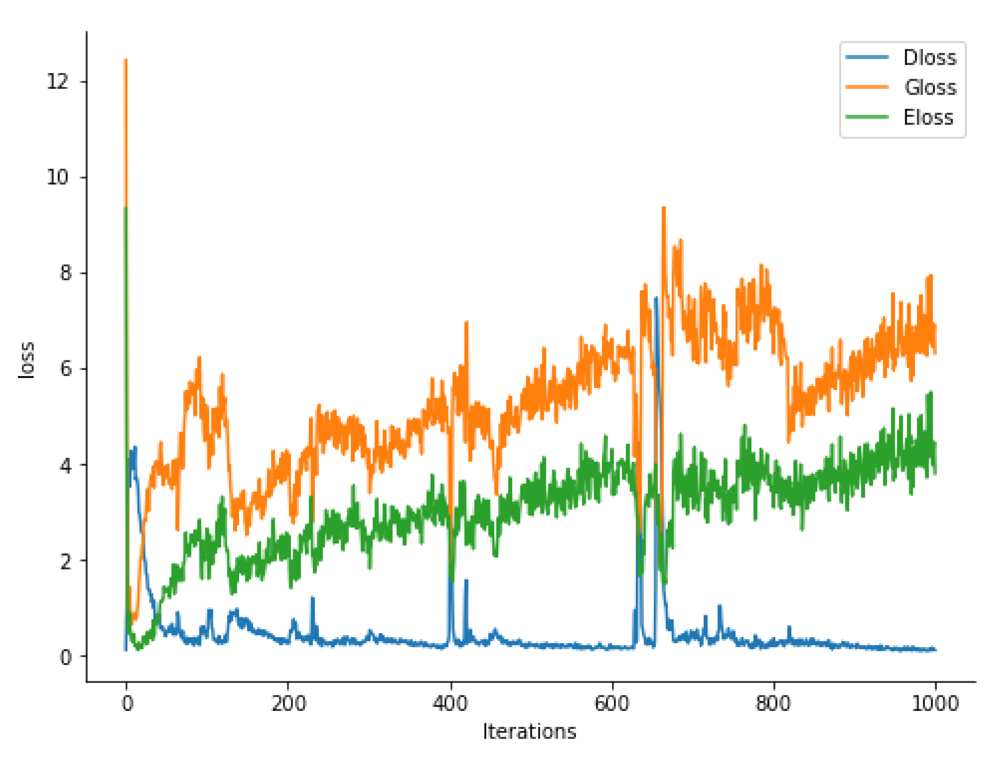
The ultimate goal of the training strategy involved in a GAN approach is for the generator and the discriminator to reach Nash equilibrium where their chosen training strategies maximize the payoffs (i.e., the generator produces the fake data as resembles as the real data while the discriminator has built up enough knowledge to distinguish the real from fake samples). In the existing GAN approaches dealing with natural images, this often requires both the generator and the discriminator to improve their capabilities at a relatively equivalent speed.

However, this training strategy often does not work in many application scenarios, because often the semantic relationships of the feature sets require to be maintained in the data set produced by the generator, and the data set being operated on in the discriminator differ from each other, which often leaves the training of the generator unstable (i.e., the loss of the generator fluctuates widely) [21].

In many cases, discriminator converges easily at the beginning of training [22], making the generator never reach its optimum. To address this issue for network intrusion detection tasks, we train the generator (and the encoder accordingly) more iterations than the discriminator. This new training strategy can prevent an optimum discriminator from appearing too early in the training stage thus keeping the training to be more balanced between the generator and discriminator.

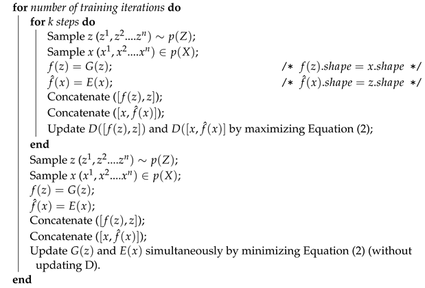
Our training strategy is depicted in Algorithm 3 where the training is processed in mini-batch. In the first stage, the discriminator is trained and updated with a batch of real samples (input from the encoder) and a batch of fake samples (input from the generator) in sequence. In the next stage, the discriminator is fixed and the encoder and the generator are trained k times. Like it was used in [20], we also adopt the “—log(D) trick” [5] to train the generator and the encoder more efficiently by flipping the target label between the generator and the encoder. For example, the input from the encoder is labeled as 1 (fake) while the input from the generator is labeled as 0 (real). Now the result of $O\left(\widehat{y}\right|y)$ is reversed which generates large gradients. This reflects the second part of an iteration in Algorithm 3 (i.e., the inner for-loop).

Training Loss Function

In many cases, Kullback–Leibler (KL) divergence or Jensen–Shannon (JS) divergence are used to measure the distance between the joint distribution of $P(x,E(x\left)\right)$ and $P\left(G\right(z),z)$ in many image-based BiGAN variants which produces the optimum, $E=G^{-1}$ and the divergence of 0. This does not work for text-based BiGAN as the divergence of the two joint distributions of $P(x,E(x\left)\right)$ and $P\left(G\right(z),z)$ cannot be computed directly but can only be approximated indirectly using the discriminator. With this understanding, we use the cross-entropy to approximate the divergence. Equation (3) depicts the cross-entropy of two distribution $P\left(x\right)$ and $Q\left(x\right)$ and where $P\left(x\right)$ is the actual target (0 or 1) and the $Q\left(x\right)$ is the joint distribution of $P(x,E(x\left)\right)$ or $P\left(G\right(z),z)$.

$$H(P,Q)={\mathbb{E}}_{x\sim P}[logQ\left(x\right)]=-\sum _{x=1}^{n}P\left(x\right)log\left(Q\left(x\right)\right)$$

(3)

where $P\left(x\right)$ is the actual target (0 or 1) and the $Q\left(x\right)$ is the predict. Now we can unify the updating of the encoder, generator, and discriminator to minimize the result of this loss.

Algorithm 3: Training Phase of our proposed method

In the first stage of training, the discriminator is updated in iteration: if the input comes from the encoder, the second part of the objective function (2) becomes 0. maximizing the first part of the objective function equals to minimize the cross-entropy values between $P(x=1)$ and $Q\left(x\right)$ as seen in the following Equation:

$$H(1,Q)=-logD(x,E(x\left)\right)$$

(4)

If the input comes from the generator, the first part of the objective function (2) becomes 0. The second part of the objective function is equivalent to minimizing the cross-entropy values between $P(x=0)$ and $Q\left(z\right)$, as seen in the following Equation:

$$H(0,Q)=-logD\left(G\right(z),z)$$

(5)

When training the generator and the encoder, the parameters of the discriminator is fixed. In fact, the two modules are trained separately: the encoder is trained in the encoder-discriminator joint structure while the generator is trained in the generator-discriminator joint network. Since the labels of input are swapped, the target label will set to be 0 when the input is a real sample x∼$p\left(x\right)$. Updating the encoder is to minimize the cross-entropy between $P(x=0)$ and $Q\left(x\right)$:

$$H(0,Q)=-logD(x,E(x\left)\right)$$

(6)

On the other hand, updating the generator is to minimize the cross-entropy between $P(x=1)$ and $Q\left(x\right)$:

$$H(1,Q)=-logD\left(G\right(z),z)$$

(7)

4.3. Testing Phase

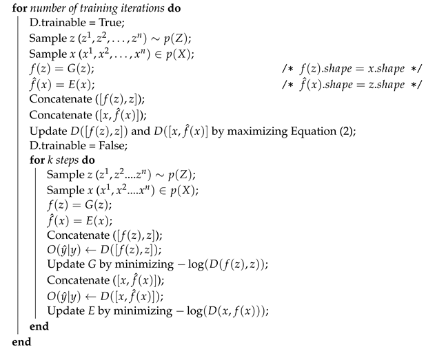
After the training is completed, the discriminator has full knowledge of the joint distribution of normal samples. The output probability is close to 0 when the input of the encoder is normal samples, and far from 0 if the input is anomalous samples.

This knowledge at the discriminator is used in the testing phase. If the probability value is greater than a given $\kappa$, the discriminator has high confidence to label the test sample anomalous. We follow the convention to set $\kappa =0.5$ to use it as a marker to decide whether a network traffic record in the testing set is normal or anomalous. In another words, if $O\left(\widehat{y}\right|y)>0.5$, the discriminator in our proposed model mark the inputted test data point as an anomaly. This evaluation process is depicted in Algorithm 4.

Algorithm 4: Testing Phase of our proposed method

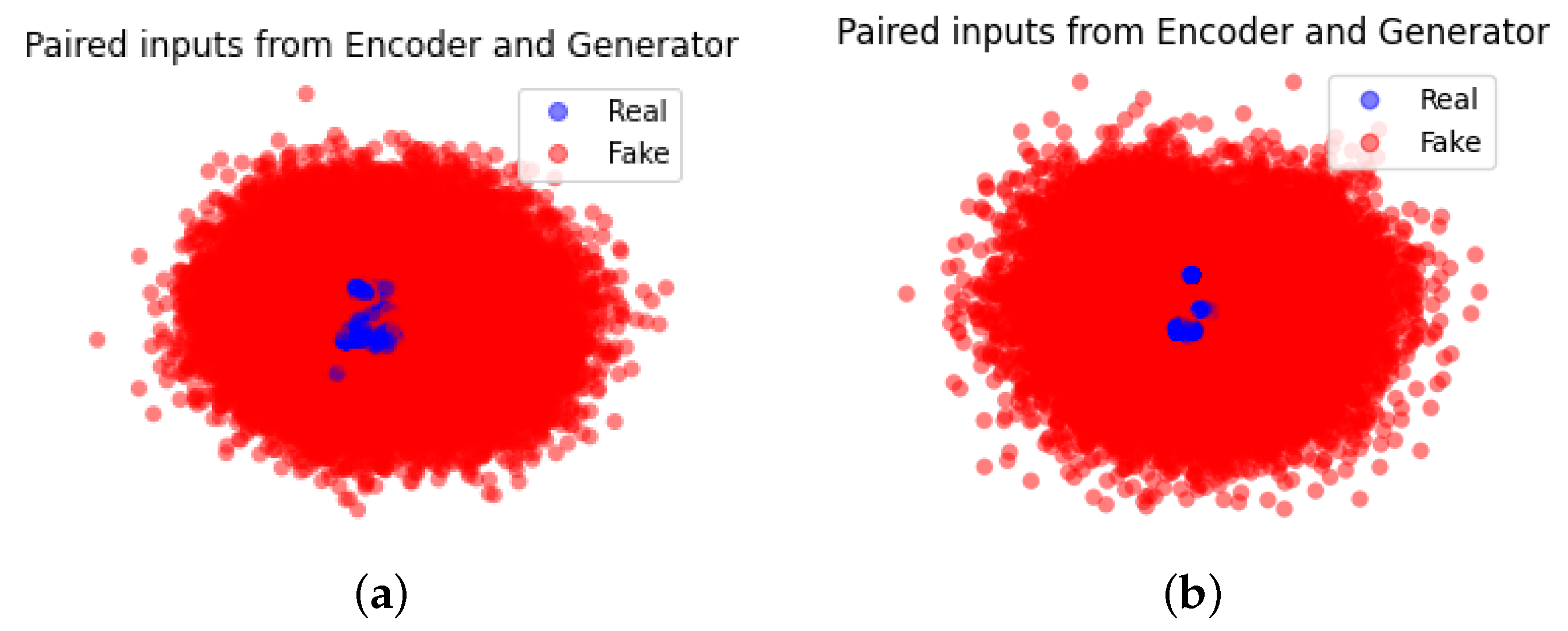
The intuition behind this one-class classifier is whether a network traffic sample in the test data set is normal or anomalous is following. In the training phase, the encoder only operates on normal data samples with its data distribution represented by $p\left(x\right)$ and learns the distribution in the latent representation ($p\left(E\right(x)$). Now at the test phase where the encoder receives not only normal data samples but also anomalous data samples ($X^{\prime }$), the encoder still compresses the anomalous inputs to the same latent distribution ($p\left(E\right(x)$). Since the anomalous input samples falls outside the “normal distribution” ($X^{\prime }\notin p\left(x\right)$), their latent representations ($p(E\left(X^{\prime }\right)$) are most likely outliers, that is $p(E\left(X^{\prime }\right))\notin p(E\left(x\right))$. This enables the discriminator to produce a high probability value close to 1, which now the discriminator can mark them as anomalies.

4.4. Putting It Together

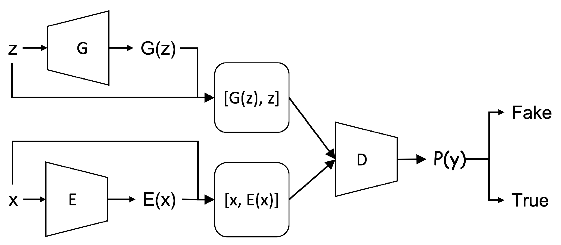
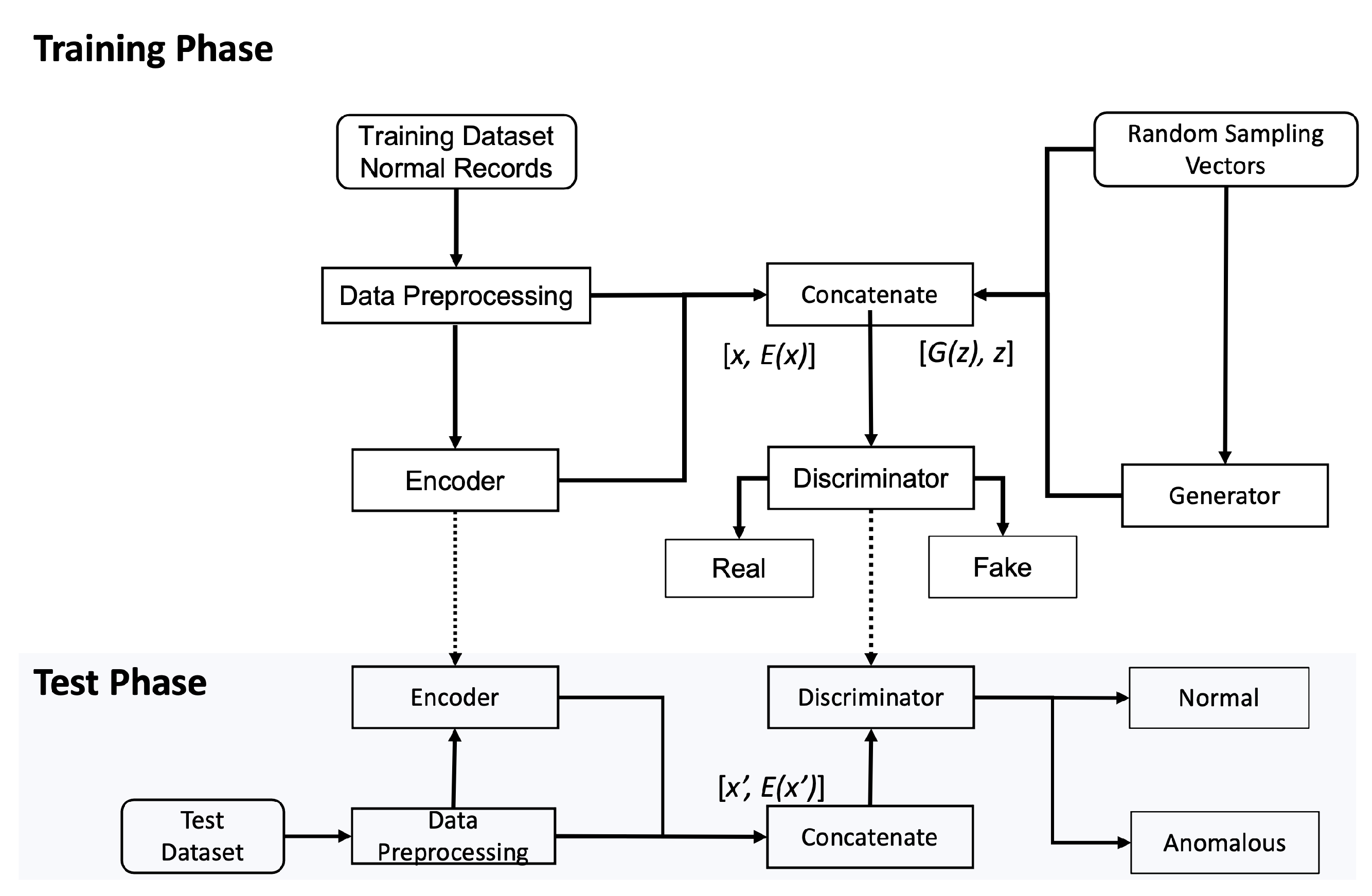
Figure 3 illustrates our proposed approach.

Figure 3. Flowchart of our proposed approach.

During the training phase, a normal traffic sample x is processed to feed into the encoder as the input. The encoder maps x to latent representations $E\left(x\right)$ as the output. Their concatenation $[x,E(x\left)\right]$ becomes an input to the discriminator representing real data, labeled with the value 0.

The generator draws a low dimensional vector z and fills it with random values derived from a standard distribution to generate synthetic samples $G\left(z\right)$. Their concatenation $\left[G\right(z),z]$ becomes another input to the discriminator representing fake data, labeled with the value 1.

The discriminator outputs a probability $O\left(\widehat{y}\right|y)$ to estimate whether the input is a “real” sample or a “fake” sample. For example, if $O\left(\widehat{y}\right|y)\approx 0$, the discriminator predicts that the input is the real sample from the encoder, otherwise, the input is the fake sample from the generator. The cross-entropy is used as the unified loss function to update all the three modules in our proposed model while flipping labels provide a strong gradients signal for updating the encoder and the generator.

During the testing phase, the testing samples ($x^{\prime }$) containing both normal and abnormal traffic samples are inputted to the encoder which outputs a low dimensional feature representation of these inputs $E\left(x\right)$. The paired vector $[x,E(x\left)\right]$ becomes the input to the discriminator. The discriminator, by now well trained to see which probability values to associate with the real or fake samples, produces a probability value of each input sample, and predicts whether the input is normal or anomalous since the anomalous input produces considerably dissimilar probabilistic values observed during the training on normal samples.

5. Data and Preprocessing

5.1. Datasets

We used two different datasets in our evaluations, the NSL-KDD dataset and the CIC-DDoS2019 dataset, respectively. These datasets are not a perfect representative of existing real networks. However, because of the lack of public datasets available for building new models for network intrusion detection, they have been widely used as an effective benchmark to compare different intrusion detection methods. We use two full subsets of the NSL-KDD dataset where the KDDTrain+ contains the dataset that can be used for training the model while KDDTest+ contains the dataset for testing the model. Among the total of 125,973 records in the KDDTrain+ dataset, a total 67,343 of records are considered as normal samples while a total of 58,630 records are categorized as abnormal samples. Similarly, among the total of 22,544 records in the KDDTest+ dataset, the records are grouped into a total of 9711 normal samples and 12,833 abnormal samples, respectively. The details of NSL-KDD is shown in Table 1.

Table 1. Records of two NSL-KDD datasets: KDDTrain+ and KDDTest+.

NSL-KDD	Total	Normal	Others
KDDTrain+	125,973	67,343	58,630
KDDTest+	22,544	9711	12,833

Each traffic record in the NSL-KDD dataset contains a total of 41 features, including 38 numeric (e.g., “int64” or “float64”) and 3 symbolic values (e.g., “object”). Table 2 shows the details of all 41 features including the name of the feature and data type.

Table 2. NSL-KDD dataset features: 38 numeric and 3 symbolic.

No	Features	Type	No	Features	Type
0	duration	int64	21	is_guest_login	int64
1	protocol_type	object	22	count	int64
2	service	object	23	srv_count	int64
3	flag	object	24	serror_rate	float64
4	src_bytes	int64	25	srv_serror_rate	float64
5	dst_bytes	int64	26	rerror_rate	float64
6	land	int64	27	srv_rerror_rate	float64
7	wrong_fragment	int64	28	same_srv_rate	float64
8	urgent	int64	29	diff_srv_rate	float64
9	hot	int64	30	srv_diff_host_rate	float64
10	num_failed_logins	int64	31	dst_host_count	int64
11	logged_in	int64	32	dst_host_srv_count	int64
12	num_compromised	int64	33	dst_host_same_srv_rate	float64
13	root_shell	int64	34	dst_host_diff_srv_rate	float64
14	su_attempted	int64	35	dst_host_same_src_port_rate	float64
15	num_root	int64	36	dst_host_srv_diff_host_rate	float64
16	num_file_creations	int64	37	dst_host_serror_rate	float64
17	num_shells	int64	38	dst_host_srv_serror_rate	float64
18	num_access_files	int64	39	dst_host_rerror_rate	float64
19	num_outbound_cmds	int64	40	dst_host_srv_rerror_rate	float64
20	is_host_login	int64

The CIC-DDoS2019 dataset contains a total of 13 different types of DDoS attacks. It is a highly imbalanced dataset with more than 50 million attack samples while proportionally a very few BENIGN samples. In our experiment, we extracted all 56,425 unique benign samples and made them as the training set. We randomly sampled 5% of attack samples and some portions of the benign samples and made them the test set to evaluate our approach. Table 3 shows the number of sample sizes used for training and test.

Table 3. Records of CIC-DDoS2019 training and test set.

CIC-DDoS2019	Total	BENIGN	ATTACKS
Training	56,425	56,425	-
test	977,830	2811	975,019

5.2. Data Preprocessing

For the NSL-KDD dataset, we first encoded 3 symbolic features using one-hot-encoding and converted them into 84 unique features. This resulted in the input source of the encoder having a total of 122 features. After applying one hot-encoding, outliers are removed following the operation applied in [14]—that is, the instances that contain the top 5% values of any feature (including encoded categorical features) are disposed of. By removing outliers after the one hot-encoding, all features are now treated equally, regardless of their data types, thus reducing the bias associated with an imbalanced number of particular data types. Furthermore, the Minmax Scaler is used to normalize the data into the range of [0, 1].

As for the input to the generator, the vectors are randomly drawn from a normal distribution of the real dataset to match the size of the latent space dimension (e.g., 10 input vectors according to the latent space with the size of 10). The output size of the generator is decided according to the size of features (e.g., 122 neurons according to the total size of features in the training dataset). As our encoder does the inverse mapping of the generator, the input size corresponds to the size of the total features (e.g., 122) while the output size is the size of the latent space (e.g., 10). The input size of the discriminator is equal to the concatenation of the output of the generator and its input (e.g., 132) while the output size is a single neuron (e.g., as a binary classifier). Figure 4 illustrates the data flow of the three components of our BiGAN model based on the analysis of the NSL-KDD dataset.

Figure 4. BiGAN data flow. Encoder: input dimensions (122), output dimensions (10); Generator: input dimensions (10), output dimensions (122); Discriminator concatenates the input and output of Encoder or Generator to form the input and functions as a binary classifier.

As for the CIC-DDOS2019 dataset, the preprocessing includes feature reduction, outlier removal, and data normalization, similar to the process of NSL-KDD. In the feature reduction phase, we first drop uninformative (e.g., NaN) and all-zero features. We encoded the “protocol” as a categorical feature since it only contained three values (i.e., 0, 6, 17 which represent HOPOPT, TCP, and UDP, respectively) which were eventually encoded as three individual features. In the outlier removal phase, we use the same strategy to remove the top 5% values of all features and therefore select only 29,731 BENIGN samples for training. Then, we normalize the data to the range of [0, 1].

6. Experimental Results

6.1. Setup Environment

Our experiments were carried out on the Kaggle platform using GPU for model training. The system setup is collected in Table 4 while the hyper-parameters we used in our study are shown in Table 5. (Source code is available at https://github.com/cyberteamnz1/GAN-Anomaly-Detection, accessed on 1 May 2022).

Table 4. Implementation environment specification.

Unit	Description
Processor	2 Cores, 2.0 Ghz
GPU	Tesla P100
RAM	16 GB
OS	Linux 5.10.68+
Packages used	TensorFlow 2.6.0

Table 5. Training parameters.

Parameters	Values	Description
Batch Size	64	The number of training examples in one forward/backward pass
Learning rate	0.002	Learning rate is used in the training of neural networks—range between 0.0 and 1.0.
N-iterations	1000	Total numbers of iterations in the training process
Steps	5	The compensated training iterations for Generator and Encoder

6.2. Performance Metrics

We use the classification accuracy, precision, recall, and F1 score as the performance metrics to evaluate the performance effectiveness of our proposed model. We use: True Positive (TP) indicates the number of correctly predicted anomalies, True Negative (TN) indicates the number of correctly predicted normal instances, False Positive (FP) indicates the number of normal instances that are misclassified as anomalies, and False Negative (FN) indicates the number of anomalies that are misclassified as normal.

We use True Positive Rate (also known as Recall) to estimate the ratio of the correctly predicted samples of the class to the overall number of instances of the same class using Equation (8). Typically, the higher TPR $\in [0,1]$ indicates the good performance of the model.

$$TPR\left(Recall\right)=\frac{TP}{TP+FN}$$

(8)

We use Precision to measure the quality of the correct predictions which is computed by the ratio of correctly predicted samples to the number of all the predicted samples for that particular class as seen in Equation (9).

$$Precision=\frac{TP}{TP+FP}$$

(9)

F1-Score computes the trade-off between precision and recall. Mathematically, it is the harmonic mean of precision and recall as shown in Equation (10).

$$F1=2\times \left(\frac{Precision\times Recall}{Precision+Recall}\right)$$

(10)

Similar to F1-score, we use Accuracy (Acc) to measure the total number of data samples correctly classified in terms of all the predictions made by the model using Equation (11).

$$Acc=\frac{TP+TN}{TP+TN+FP+FN}$$

(11)

We also use the area under the curve (AUC) to compute the area under the receiver operating characteristics (ROC) curve plotting the trade-off between the true positive rate (i.e., typically depicted on the y-axis) and the false positive rate (i.e., on the x-axis across different thresholds) using Equation (12).

$$AU{C}_{ROC}={\int }_0^1\frac{TP}{TP+FN}d\frac{FP}{TN+FP}$$

(12)

6.3. Results

We report the analysis of the observation we have made during our experiments.

6.3.1. Training Loss and PCA

The training loss is an important indicator of model performance. In adversarial networks, the training loss of the discriminator is expected to be opposite to the generator in general, but both of them converge into a narrow range. In our proposed approach, we train the generator (as well as the encoder) more times to match the converging pace of the discriminator.

We take the training process of NSL-KDD dataset as an example to demonstrate the convergence. Figure 5 illustrate the trend of the training losses associated with our main components. In this experiment, the training of the encoder, generator, and discriminator has gone through 1000 iterations. As expected, the training losses for the encoder (i.e., Eloss depicted by the green line) and generator (i.e., Gloss depicted by the orange line) were not stable in the first 170 iterations but become stead when the training passed 200 iterations. As the encoder is the inverse mapping of the generator, the trend in the training loss patterns is pretty similar between the two. The training loss for discriminator (i.e., Dloss depicted by blue line) becomes stabilized much earlier only after 50 iterations, and remains steady.

Figure 5. Training losses vs. iterations. Eloss, Gloss, and Dloss represent the training loss trend of encoder, generator, and discriminator, respectively.

We also visualize the PCA results as a metric for model analysis. Figure 6 illustrates the 2-D visualization of the distribution among the normal and abnormal samples in KDDTrain+ and KDDTest+. As it illustrates, there are two distinct clusters in the KDDTrain+ dataset, one belongs to normal samples and the other belong to abnormal data samples. The feature values are pretty widely spread across each cluster both in the normal and abnormal dataset. In contrast, the clusters around normal and abnormal samples in the KDDTest+ are less distinct as there are many overlapping data points across the normal and abnormal samples. The feature distribution of the normal dataset is within a narrow range while the feature distribution of the abnormal dataset is much wider.

Figure 6. The PCA visualization of data distribution in (a) KDDTrain+ and (b) KDDTest+ dataset.

Figure 7 illustrates the PCA results of the encoder and the generator after training when: (a) represents two paired concatenated outputs when trained on the NSL-KDD dataset while (b) represents the results on the CIC-DDoS2019 dataset. As shown in the two graphs, the real samples are condensed into clusters while the generated samples surround those real samples with overlapping. This indicates that the generator can simulate the data distribution of normal/BENIGN samples of the datasets to some extent. However, the fake samples scatter around a much broader area than the real samples which can be regarded as the anomalies for the discriminator in the training process.

Figure 7. The PCA visualization of concatenated outputs of the encoder and the generator after training on (a) NSL-KDD and (b) CIC-DDoS2019.

6.3.2. Testing

The performance of our proposed model on the two datasets using the 4 performance metrics we specified earlier is depicted in Table 6. The F1-score for the NSL-KDD dataset achieves more than 92% while the CIC-DDoS2019 dataset achieves more than 99% with very competitive rates for both precision and recall. We also present the training runtime—the average time it takes for 1000 iterations in milliseconds. Note that at each iteration, the generator goes through 5 times more iterations than the discriminator as the training iteration of these two does not need to be in sync.

Table 6. Performance of our approach.

Dataset	Accuracy	Precision	Recall	F1 Score	Time ($\mathit{\mu }\pm \mathit{\sigma }$)
KDDTest+	91.12%	87.27%	98.81%	92.68%	$118\mathrm{ms}\pm 25\mathrm{ms}$
CIC-DDOS2019Test+	99.68%	99.85%	99.82%	99.84%	$59\mathrm{ms}\pm 23\mathrm{ms}$

To illustrate a more detailed analysis of the performance, the experimental results based on the confusion matrix are shown in Figure 8. For the NSL-KDD dataset shown in (a), among the total of 22,544 records used for the testing, 20,542 records were correctly classified according to their label while slightly over 2000 records (i.e., less than 9% of the total records) were misclassified as either FP (1849) or FN (153). For the CIC-DDoS2019 dataset shown in (b), among the total of 989,780 testing samples, 974,669 records were correctly classified (i.e., greater than 99% of the total records) while 3161 samples were misclassified.

Figure 8. Confusion matrix result of (a) NSL-KDD and (b) CIC-DDoS2019.

From another angle to measure the performance of our proposed model, Figure 9 depicts the AUC_ROC curve to clearly demonstrate the trade-off between true positive rate and false-positive rate. The AUC score for the NSL-KDD dataset is 0.953 which confirms that our proposed model is highly effective in accurately classifying network intrusions. On the other hand, the model reports a relatively low AUC score of 0.816 on the CIC-DDoS2019 dataset. This is due to the high false positives in the classification of BENIGN samples due to the low number of samples being trained.

Figure 9. AUC_ROC curve of our proposed model on (a) NSL-KDD and (b) CIC-DDoS2019.

6.3.3. Benchmarking with Other Similar Models

We compared the performance of our proposed model with other generative deep neural network models such as Autoencoder and GAN-based approaches test against to similar network intrusion dataset similar to the NSL-KDD dataset (e.g., KDD99). The benchmarking result is shown in Table 7. Overall, GAN-based approaches show slightly better performance in terms of different performance metrics compared to the Autoencoder-based method. Among different GAN-based methods, our proposed model shows the best performance by achieving more than 92% F1-score.

Table 7. Performance of our approach and other state-of-art approaches.

Method	Accuracy	Precision	Recall	F1 Score	Dataset
AE [23]	84.21%	87%	80.37%	81.98%	NSL-KDD
AE [15]	88.98%	87.92%	93.48%	90.61%	NSL-KDD
DAE [16]	88.65%	96.48%	83.08%	89.28%	NSL-KDD
AnoGAN [24]	-	87.86%	82.97%	88.65%	KDD99
BiGAN [9]	-	93.24%	94.73%	93.98%	KDD99
BiGAN [10]	89.5%	83.6%	99.4%	90.8%	KDD99
Our approach	91.12%	87.27%	98.81%	92.68%	NSL-KDD

7. Conclusions

In this study, we proposed a new Bidirectional GAN model more suited to detect network intrusion attacks with less training overheads and a less expensive one-class classifier. Unlike existing GANs used in natural image processing which demand a strong dependence between the generator and the discriminator to produce realistic fake images, our proposed model allows the generator and the discriminator to be trained without needing to be in sync in their training iterations. By relaxing the dependence between these two, the generator and encoder working together, we can produce more accurate synthetic text-based network traffic samples without excess training overheads of the discriminator. This approach is more suited to the network intrusion inputs that exhibit less complex feature structures with a few feature dimensions, mostly discrete feature values, and the size of input relatively smaller compared to the existing GAN variants used for anomaly detection tasks on images.

Our model is also equipped with a one-class binary classifier for the trained encoder and discriminator to use for detecting anomalous traffic from normal traffic. By offering a one-class (binary) classifier, a complex calculation involved in finding a threshold or anomaly score can be avoided.

Our proposed model, evaluated on extensive experimental results on two separate datasets, demonstrates that it is highly effective for the generator to produce a synthetic network traffic dataset that can contribute to detecting anomalous network traffic. Our benchmarking result shows that our proposed model outperformed other similar generative models by achieving more than 92% F1-score on the NSL-KDD dataset and more than 99% F1-score on the CIC-DDoS2019 dataset.

Many existing network intrusion datasets currently used to develop many deep learning models suffer from high false positives due to the presence of minority classes. To address this issue, we plan to extend our work as a general data argumentation technique to produce more synthetic data samples that resemble actual samples. We may consider employing a similarity function such as Pearson Correlation or flocking methods proposed by [25,26], or other statistical analysis methods to evaluate the similarity between the synthetic data and actual samples from many different aspects of data distribution. Eventually, we plan to test such GAN-based data augmentation technique for our previous works on DDoS attack classification [27], Android-based malware detection [28,29], or ransomware detection and classification tasks [30,31,32] by improving the quality of rare minority classes. We also plan to apply our technique for other application areas, such as finding defects in X-ray images [33] to evaluate the feasibility, extensionability, and generalizability of our approach.

References

- Jang-Jaccard, J.; Nepal, S. A survey of emerging threats in cybersecurity. J. Comput. Syst. Sci. 2014, 80, 973–993. [Google Scholar] [CrossRef]
- Ahmad, Z.; Khan, A.S.; Shiang, C.W.; Abdullah, J.; Ahmad, F. Network intrusion detection system: A systematic study of machine learning and deep learning approaches. Trans. Emerg. Telecommun. Technol. 2021, 32, e4150. [Google Scholar] [CrossRef]
- Zhu, J.; Jang-Jaccard, J.; Liu, T.; Zhou, J. Joint Spectral Clustering based on Optimal Graph and Feature Selection. Neural Process. Lett. 2021, 53, 257–273. [Google Scholar] [CrossRef]
- Kingma, D.P.; Welling, M. Auto-encoding variational bayes. arXiv 2013, arXiv:1312.6114. [Google Scholar]
- Goodfellow, I.; Pouget-Abadie, J.; Mirza, M.; Xu, B.; Warde-Farley, D.; Ozair, S.; Courville, A.; Bengio, Y. Generative adversarial nets. Adv. Neural Inf. Process. Syst. 2014, 27, 1–9. [Google Scholar]
- Schlegl, T.; Seeböck, P.; Waldstein, S.M.; Schmidt-Erfurth, U.; Langs, G. Unsupervised anomaly detection with generative adversarial networks to guide marker discovery. In Information Processing in Medical Imaging; Niethammer, M., Styner, M., Aylward, S., Zhu, H., Oguz, I., Yap, P.T., Shen, D., Eds.; Springer International Publishing: Cham, Switzerland, 2017; pp. 146–157. [Google Scholar]
- Schlegl, T.; Seeböck, P.; Waldstein, S.M.; Langs, G.; Schmidt-Erfurth, U. f-AnoGAN: Fast unsupervised anomaly detection with generative adversarial networks. Med. Image Anal. 2019, 54, 30–44. [Google Scholar] [CrossRef] [PubMed]
- Akcay, S.; Atapour-Abarghouei, A.; Breckon, T.P. GANomaly: Semi-supervised anomaly detection via adversarial training. In Computer Vision—ACCV 2018; Jawahar, C.V., Li, H., Mori, G., Schindler, K., Eds.; Springer International Publishing: Cham, Switzerland, 2019; pp. 622–637. [Google Scholar]
- Chen, H.; Jiang, L. Efficient GAN-based method for cyber-intrusion detection. arXiv 2019, arXiv:1904.02426. [Google Scholar]
- Kaplan, M.O.; Alptekin, S.E. An improved BiGAN based approach for anomaly detection. Procedia Comput. Sci. 2020, 176, 185–194. [Google Scholar] [CrossRef]
- Javaid, A.; Niyaz, Q.; Sun, W.; Alam, M. A deep learning approach for network intrusion detection system. Eai Endorsed Trans. Secur. Saf. 2016, 3, e2. [Google Scholar]
- An, J.; Cho, S. Variational autoencoder based anomaly detection using reconstruction probability. Spec. Lect. IE 2015, 2, 1–18. [Google Scholar]
- Chang, Y.; Tu, Z.; Xie, W.; Yuan, J. Clustering driven deep autoencoder for video anomaly detection. In Computer Vision—ECCV 2020; Vedaldi, A., Bischof, H., Brox, T., Frahm, J.M., Eds.; Springer International Publishing: Cham, Switzerland, 2020; pp. 329–345. [Google Scholar]
- Xu, W.; Jang-Jaccard, J.; Singh, A.; Wei, Y.; Sabrina, F. Improving Performance of Autoencoder-based Network Anomaly Detection on NSL-KDD dataset. IEEE Access 2021, 9, 140136–140146. [Google Scholar] [CrossRef]
- Sadaf, K.; Sultana, J. Intrusion Detection Based on Autoencoder and Isolation Forest in Fog Computing. IEEE Access 2020, 8, 167059–167068. [Google Scholar] [CrossRef]
- Aygun, R.C.; Yavuz, A.G. Network Anomaly Detection with Stochastically Improved Autoencoder Based Models. In Proceedings of the 2017 IEEE 4th International Conference on Cyber Security and Cloud Computing (CSCloud), New York, NY, USA, 26–28 June 2017; pp. 193–198. [Google Scholar] [CrossRef]
- Zenati, H.; Foo, C.S.; Lecouat, B.; Manek, G.; Chandrasekhar, V.R. Efficient gan-based anomaly detection. arXiv 2018, arXiv:1802.06222. [Google Scholar]
- Mohammadi, B.; Sabokrou, M. End-to-End Adversarial Learning for Intrusion Detection in Computer Networks. In Proceedings of the 2019 IEEE 44th Conference on Local Computer Networks (LCN), Osnabrueck, Germany, 14–17 October 2019; pp. 270–273. [Google Scholar] [CrossRef] [Green Version]
- Dumoulin, V.; Belghazi, I.; Poole, B.; Mastropietro, O.; Lamb, A.; Arjovsky, M.; Courville, A. Adversarially learned inference. arXiv 2016, arXiv:1606.00704. [Google Scholar]
- Donahue, J.; Krähenbühl, P.; Darrell, T. Adversarial feature learning. arXiv 2016, arXiv:1605.09782. [Google Scholar]
- Arjovsky, M.; Bottou, L. Towards Principled Methods for Training Generative Adversarial Networks. arXiv 2017, arXiv:stat.ML/1701.04862. [Google Scholar]
- Berthelot, D.; Schumm, T.; Metz, L. Began: Boundary equilibrium generative adversarial networks. arXiv 2017, arXiv:1703.10717. [Google Scholar]
- Ieracitano, C.; Adeel, A.; Morabito, F.C.; Hussain, A. A novel statistical analysis and autoencoder driven intelligent intrusion detection approach. Neurocomputing 2020, 387, 51–62. [Google Scholar] [CrossRef]
- Zenati, H.; Romain, M.; Foo, C.S.; Lecouat, B.; Chandrasekhar, V. Adversarially Learned Anomaly Detection. In Proceedings of the 2018 IEEE International Conference on Data Mining (ICDM), Singapore, 17–20 November 2018; pp. 727–736. [Google Scholar] [CrossRef] [Green Version]
- Forestiero, A. Metaheuristic algorithm for anomaly detection in Internet of Things leveraging on a neural-driven multiagent system. Knowl. Based Syst. 2021, 228, 107241. [Google Scholar] [CrossRef]
- Forestiero, A. Bio-inspired algorithm for outliers detection. Multimed. Tools Appl. 2017, 76, 25659–25677. [Google Scholar] [CrossRef]
- Wei, Y.; Jang-Jaccard, J.; Sabrina, F.; Singh, A.; Xu, W.; Camtepe, S. Ae-mlp: A hybrid deep learning approach for ddos detection and classification. IEEE Access 2021, 9, 146810–146821. [Google Scholar] [CrossRef]
- Zhu, J.; Jang-Jaccard, J.; Watters, P.A. Multi-Loss Siamese Neural Network with Batch Normalization Layer for Malware Detection. IEEE Access 2020, 8, 171542–171550. [Google Scholar] [CrossRef]
- Zhu, J.; Jang-Jaccard, J.; Singh, A.; Watters, P.A.; Camtepe, S. Task-aware meta learning-based siamese neural network for classifying obfuscated malware. arXiv 2021, arXiv:2110.13409. [Google Scholar]
- Zhu, J.; Jang-Jaccard, J.; Singh, A.; Welch, I.; AI-Sahaf, H.; Camtepe, S. A Few-Shot Meta-Learning based Siamese Neural Network using Entropy Features for Ransomware Classification. arXiv 2021, arXiv:2112.00668. [Google Scholar] [CrossRef]
- McIntosh, T.R.; Jang-Jaccard, J.; Watters, P.A. Large Scale Behavioral Analysis of Ransomware Attacks. In Neural Information Processing; Cheng, L., Leung, A.C.S., Ozawa, S., Eds.; Springer International Publishing: Cham, Switzerland, 2018; pp. 217–229. [Google Scholar]
- McIntosh, T.; Jang-Jaccard, J.; Watters, P.; Susnjak, T. The Inadequacy of Entropy-Based Ransomware Detection. In Neural Information Processing; Gedeon, T., Wong, K.W., Lee, M., Eds.; Springer International Publishing: Cham, Switzerland, 2019; pp. 181–189. [Google Scholar]
- Feng, S.; Liu, Q.; Patel, A.; Bazai, S.U.; Jin, C.K.; Kim, J.S.; Sarrafzadeh, M.; Azzollini, D.; Yeoh, J.; Kim, E.; et al. Automated pneumothorax triaging in chest X-rays in the New Zealand population using deep-learning algorithms. J. Med. Imaging Radiat. Oncol. 2022, in press. [Google Scholar] [CrossRef]
Publisher’s Note: MDPI stays neutral with regard to jurisdictional claims in published maps and institutional affiliations. |
© 2022 by the authors. Licensee MDPI, Basel, Switzerland. This article is an open access article distributed under the terms and conditions of the Creative Commons Attribution (CC BY) license (https://creativecommons.org/licenses/by/4.0/).