3.1. Industrial Data
This study was conducted within a large electronics manufacturer that supplies assembled components (mainly automotive instrument clusters) to some of the most recognized brands in the automobile industry. The assembly of a cluster is an extensive process with multiple assembly stages. In this work, we focus on one of the final phases in the process, where the plastic housing is combined with either the printed circuit boards (PCB) or other plastic parts. Bonding plastics or electronics to plastics can be achieved via a multitude of techniques that involve glue, welding, or the use of screw fasteners. For the remainder of the article, we optimize the validation process of screw tightening processes, which makes use of threaded fasteners as the bonding mechanism for the units.
Validating a fastening procedure can be challenging, since it involves several real-time variables. The manufacturing experts take their knowledge into account and leverage the information provided by the handheld driver manufacturers to overcome most of the problems inherent to the usage of this bonding technique. Despite the efforts to mitigate most failure modes with approaches such as sequence based fastening, some deviations still occur on the shop floor and the control mechanisms must be able to signal them fast and accurately.
The plant standardizes most production lines to follow the most efficient layout in terms of assembled clusters throughput per hour. Individually, each assembly station follows a strict set of rules that check for violations in the correctness of the fastening sequence. The assembly process starts with the operator inserting the raw plastic housing in a assembly jig. This jig is designed with the “poka yoke” principle [
13], which prevents wrong or misaligned parts from being loaded into the assembly jig. A scanner installed in a favorable position reads the imprinted identification code and verifies if the product successfully passed the previous checkpoints and if the station is capable of executing this assembly stage. The correct screw tightening program is then loaded onto the handheld tool. This stage is fundamental because different variants of the same part can be produced on the same machine where the threaded holes can be of different dimensions or be located in different places. The settings specified in this program are also used as a baseline to compare against the real values produced by the machine. The operator then guides the handheld driver to a feeder which is always on and not controlled by the program. Once a screw is loaded on the screwdriver bit, the operator is instructed to follow a predefined sequence with the aid of instructions carefully illustrated on a monitor located above the assembly station. Each inserted screw results in a good or fail (GoF) status message, presented on the screen which indicates whether the fastening succeeded or not. Simultaneously, the produced data is stored locally on a
.csv file. Depending on the result, two different courses of action can be performed: on failure—the operator is instructed to stop the procedure; on success—the data is uploaded to a remote server where it will be thoroughly analyzed by an expert tool that compares the produced data against a defect catalog. If no defect is detected, the operator is instructed to proceed to the next unit. This new control flow differs from the one presented in our past work [
1], as the manufacturing experts deemed it more important to detect false negatives (assembly cycles considered good but are not) than further analysis of faulty units that would have to restart the assembly process.
Regardless of the outcome, new files are made available on a remote data-server (separate from the one running the expert tool) and are then subjected to Extract, Transform, and Load (ETL) processes to make data easier to be worked on. Up until this stage, we have no control over the generated data stream. We are currently reading this pre-processed data using
.parquet files partitioned by date but this process is undergoing some structural changes which will fundamentally change the way we access new data, making it available through Solace, an event broker tool [
14].
Table 1 outlines some of the variables collected for each assembly process. The granularity of the data collated depends on a diverse set of factors, such as the type of the machine in use or the type of product being produced. Some machines do not even support the computation of the variables collected once per fastening (e.g., DTM based attributes). Nevertheless, all machines support the collection of angle and torque values. For each
i process, there is a real-time generation of several
values, where
denotes the total number of observations where each part number can produce a different
value. For each unique combination of
i and
k values, the machine collects hundreds of angle (
) and torque (
) measurements. It should be highlighted that while there is no direct temporal variable in the collected attributes, the angle (
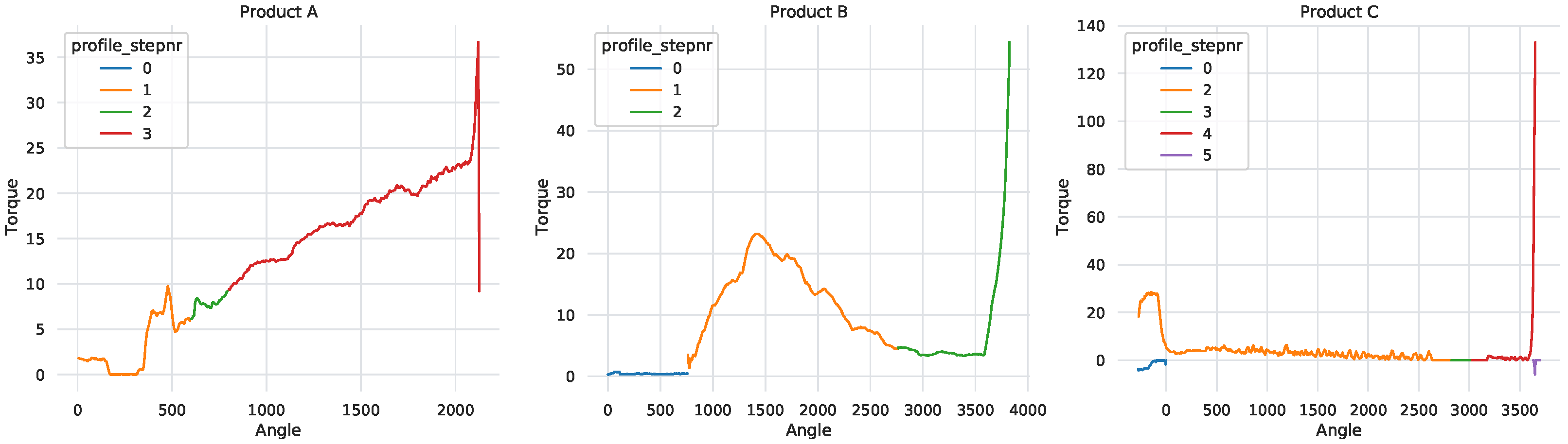
) attribute can be used as a sequential temporal measure of the fastening cycle. In effect, the angle represents the rotation made by the screw during the fastening process. Thus, as the angle value increases, the closer the screwing cycle is to reaching its end, which is often marked by an abrupt increase/decrease of the torque value (e.g., screw head fastened to the surface).
A typical screwdriving cycle is characterized by four stages as per described in
Table 2. Should a process be successful (
Figure 1), the unit needs to undergo all steps and meet the transition conditions of each sequentially. During the initial stage (step 0), the screwdriving machine rotates counterclockwise in an attempt to latch to the screw head. Although this step is already part of the assembly process it is not relevant for the current analysis and some machines do not even report it. The remaining three steps represent mechanical milestones for the correct fixation of a screw to a plastic housing. There are some specific situations where a successful procedure skips or adds an additional step. The main reason for this behavior is related to the mechanical properties of the bonding units and the capabilities of each assembly station. For example, the DTM attribute is not calculated if the handheld driver does not support such a feature. For all others, the tool estimates the clamping angle and torque for the fastening and then compares them to the actual values (represented by
screw_dtm_clamp_angle and screw_dtm_clamp_torque). These are some of the computations the assembly machine executes to assess whether a process was finalized successfully or not, returning a GoF label (attribute
screw_gof).
Despite using one-class algorithms and selecting the angle–torque pairs as our input features, the screw_gof variable, denoted as for the i-th screw tightening process, is required during the data preparation step. Not only is it used to separate good from bad fastening cycles, it also serves as our target variable during the model evaluation stage. These labels are provided by the screwdriver and are computed by comparing the curve signature against a predefined set of static rules. Although these rules are created and tested by manufacturing experts, some cycles end up being misclassified. These rare occurrences are usually reported and handled as fast as possible. However, and considering the nature of this big data problem, it is not time- and computationally feasible to verify all assembly cycles that are part of our dataset. Instead, we assume that these occurrences are very rare and thus that they do not impact on our anomaly detection training and evaluation procedures.
Table 3 describes the more recent and larger dataset that is explored in this paper. In the table, the product names were anonymized for confidentiality reasons (termed here as A, B, and C). These were selected based on their availability and in an attempt to cover a diversity within the universe of products fabricated by the analyzed manufacturer. Each product is composed of multiple
part_numbers and is comprised of multiple fastening cycles that share similar characteristics (e.g., angle–torque signature). For each individual family, in this paper we collected two months worth of data (from February to March 2021), which result in a total of 23,790 unique serial numbers and roughly 26.9 million individual observations (67,337 fastening cycles times 400 data points per screw). As the research literature suggests, datasets in this domain are usually highly unbalanced. In our case, there is only a tiny percentage of faulty processes (e.g., 0.2% for Product A). Moreover, on average, there are around
= 400 records (angle–torque pairs) per cycle.
3.2. Anomaly Detection Angle–Torque Approach
Given the important of the screw tightening anomaly detection task, several experiments were previously conducted by the manufacturing experts. A large range of experiments were held, including the application of batch process monitoring procedures [
15]. However, this industrial anomaly detection task is non-trivial. Unlike other types of processes (e.g., chemical reactions), there can be “normal” abrupt changes in the torque values, as shown in
Figure 1 in terms of the final angle–torque curve for Product A. In effect, inefficient results were achieved when adopting the batch process monitoring attempts. Nevertheless, in one of their attempts, the experts conducted a principal component analysis (PCA) that supported our assumption that angle–torque pairs are fundamental to evaluate screwing processes. Moreover, when we started our research, we performed an initial set of experiments using a larger number of input variables (from
Table 1). Yet, the ML models (e.g., LOF, IForest, AE) obtained much worst class discrimination results while requiring an expensive computational effort. In some cases, such as when using LOF, the computational training process even halted due to an out-of-memory issue. Based on these results, we then opted to focus on the low-dimensional angle–torque input data approach, which provided better results with a much lower computational effort. Thus, in this work we developed two ML algorithms (IForest and AE) that make use of two data features (angle and torque values) as the input values, producing then an anomaly decision score (
d). It should be noted that during training, the ML algorithms are only fed with normal instances.
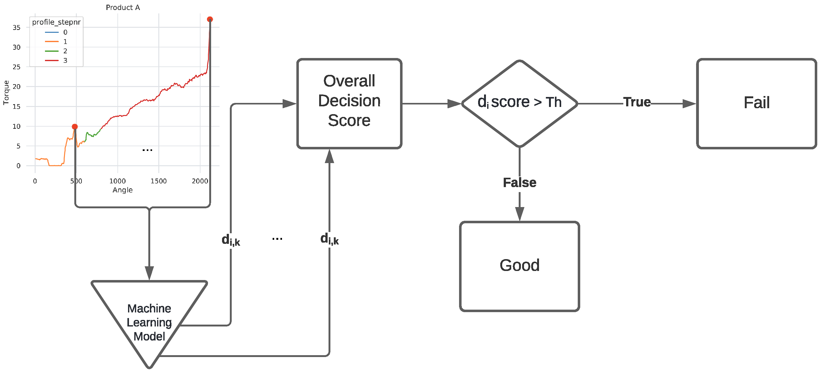
Considering that each fastening cycle is comprised of
angle–torque observations, the output of each detection model will contain
anomaly decision scores, where
i denotes the
i-th screw being evaluated. The overall decision score (
) is computed by averaging each individual score such that
. For each unique
i value, the resulting score (
) can be compared to a target label of a test set (
), making the computation of the Receiver Operating Characteristic (ROC) curve [
16] possible. Given that human operators require a class label, a fixed
threshold value is adopted such that for the
i-th output is considered anomalous when
. The overall procedure used to compute the final screw classification score (
) is shown in
Figure 2.
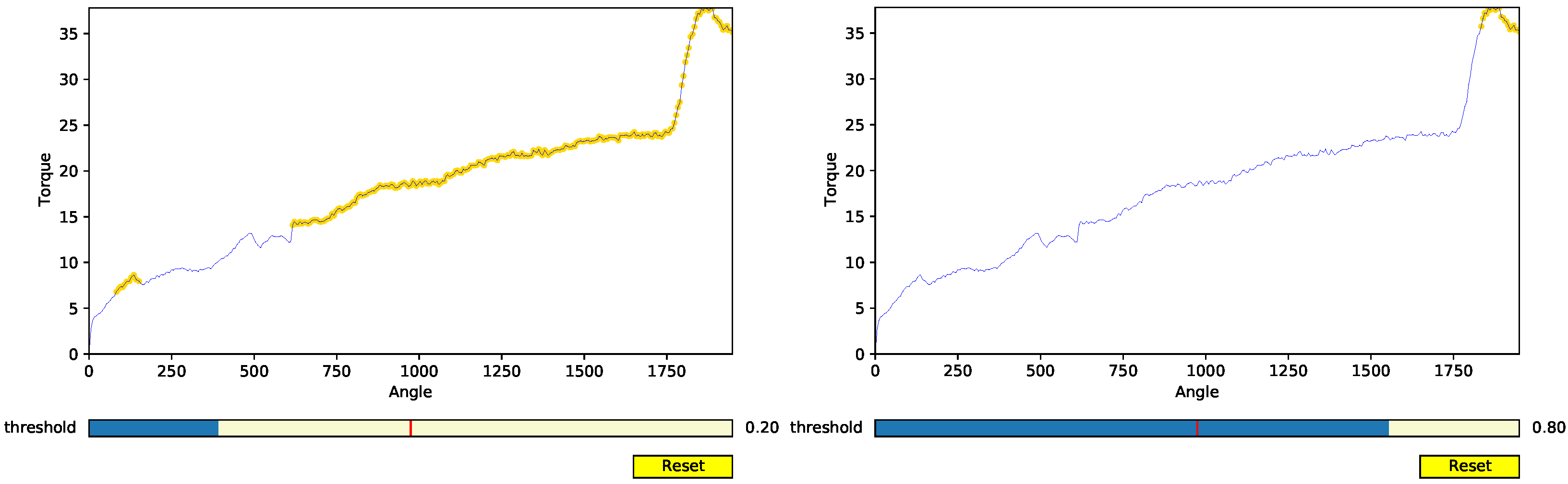
Selecting the most appropriate requires either domain knowledge or a semi-automatic selection of the best specificity–sensitivity trade-off of a ROC curve generated using a validation set (with labeled data). In this work, we assume the usage of domain knowledge, as provided by the screw tightening human operators. To support the expert value selection, we propose a specialized XAI interactive visual tool that includes a threshold selection mechanism. The tool allows a finer control over the threshold selection process, allowing experts to manually specify individual thresholds for different families of products and to easily identify problematic angle–torque regions within the screw tightening profile curves.
The data collected during each individual assembly process contains 44 unique attributes spanning three granularity levels.
Table 1 summarizes the 16 attributes related to the actual fastening process, while the remaining 28 features are used by the assembly management systems. As described in
Section 3.1, each process is composed of multiple observations of angle–torque pairs (
-
) and the torque gradient between two consecutive angle values is grouped by step number. Each step is comprised of multiple fine-grained observations, the total angle and torque for the given step. Subsequently, each step is grouped under a specific fastening identifier, which, alongside the aforementioned data, reflects the whole industrial screw tightening process.
While there is a large number of attributes, several experiments were conducted beforehand by manufacturing experts to try and address the problem currently being studied. Experts designed a multitude of experiments using multivariate techniques which proved to be inefficient and incapable of discriminating good from bad screwing cycles. For confidentiality reasons the results of such experiments can not be made public. In one of their runs, the conducted Principal Component Analysis (PCA) further supported our hypothesis that angle–torque pairs contain the bulk of the information necessary to evaluate screwing processes. Additionally, during the set-up of our previous work [
1] we composed a group of experiments with multiple combinations of variables and encoding techniques (such as one-hot encoding) which not only increased the overall model complexity but proved to add no extra capacity to our models. As such, and given the previously obtained results using older screw tightening data it was found that the low-dimensional angle–torque input data provided a better anomaly detection performance while requiring much less computational effort. Thus, all screw anomaly methods described in this work assume just two input values: the simpler angle–torque pairs
for each
example.
3.3. Machine Learning Models
In our previous work [
1], we compared several ML algorithms for screw tightening anomaly detection: three unsupervised algorithms, namely, LOF, IForest, and a deep AE; and the Random Forest (RF) supervised learning algorithm.
The
LOF is a density-based algorithm [
5] that heavily depends on K-nearest neighbors [
17]. It is designed as local because it depends on how well isolated an object is from the surrounding neighborhood. Instead of classifying an object as being an outlier or an inlier, an outlier factor is assigned describing up to which degree the object differs from the rest of the dataset. It should be noted that LOF can be used to detect both local and global outliers. Moreover, it can be trained with multi-class instances. In this paper, in order to provide a fair comparison, we only use normal examples to fit the model, where the outlier factor score is directly used as the anomaly decision score (
). For benchmarking purposes, we also considered the RF model, which requires labeled training data and that is build in terms of a large number of decision trees, which are then combined together as an ensemble to get more accurate and reliable predictions [
18].
In this work, we focus more on two unsupervised learning models that provided competitive results in our previous work [
1]: IForest and AE. All anomaly detection methods were coded using the Python language. The LOF, IForest and RF methods assumed the
scikit-learn module implementation [
19], while the AE was developed using the
TensorFlow library [
20]. In order to provide a fair comparison, whenever possible we adopted the default hyperparameter values assumed by the
scikit-learn and
TensorFlow implementations. Before feeding the models, the angle–torque training data were normalized by using the
MinMaxScaler procedure of the
sklearn library, scaling all inputs within the range [0, 1].
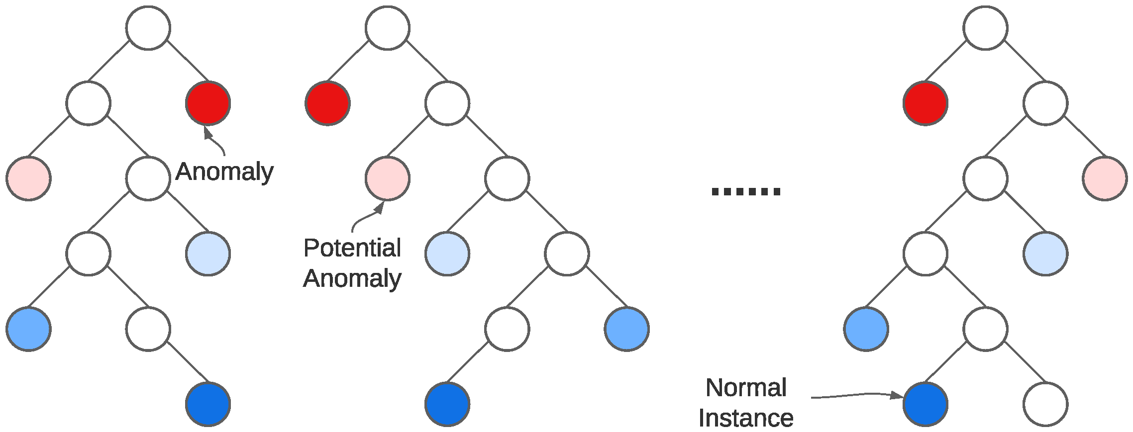
Isolation forest is an anomaly detection algorithm which, as the name indicates, uses the isolation principle to classify data as anomalous rather than modeling normality. It leverages the power of smaller decision trees combining them into a single, more capable architecture. As it makes no use of labeled data, it is an unsupervised model. It operates based on the principle that anomalies are few and numerically different from normal instances. This forces anomalous instances to be isolated easier (separated from all other instances) than normal data. Using these principles as foundation, a tree structure is created in an attempt to isolate every single instance by applying multiple splits with random parameters and then assessing on their normality. Anomalous observations with fewer attributes capable of describing them tend to be positioned closer to the root of the tree. This structure is usually regarded as an
Isolation Tree (or
iTree) and is the main component of anomaly detection of this algorithm. As such, an IForest [
21] is an ensemble of iTrees that when combined can discriminate between good and bad data.
Figure 3 summarizes the working principle of this algorithm, where the data points with shorter average path lengths are indicated as anomalies. On the other side of the spectrum, data points with bigger average path lengths are considered normal. Data points which fall in between these too extremities are classified as potential anomalies. These distances are computed and expressed by
scikit-learn as an anomaly score ranging from
−1 (highest abnormal score) to
= 1 (highest normal score), where
denotes the IForest output for the
k-th angle–torque pair of the
i-th screw tightening instance. In order to compute an anomaly probability, we rescale the IForest score by computing
.
Unlike the IForest, an AE is a type of artificial neural network that learns normality rather than computing abnormality scores. The AE is comprised of two main stages: an initial stage where it learns a representation for a set of data (encoding), typically by reducing the input data (the number of features describing the input data) and is usually unaffected by noise; and a decoding stage, in which the model tries to reconstruct the input signal. This neural network architecture imposes a bottleneck out of the encoding stage (which forces dimensionality reduction), resulting in a compact knowledge image of the original input, usually referred to as latent space. When applied to the specific case of anomaly detection, the architecture accepts normal data as input and then attempts to produce
outputs which should be identical to the input pair
, where
denotes the angle and
the torque for the
k-th measurement of the
i-th screw tightening instance. To ascertain the quality of this reconstruction, on each new
instance we compute its Mean Absolute Error (MAE) [
6], formulated as follows:
The reconstruction MAE is used as the anomaly decision score
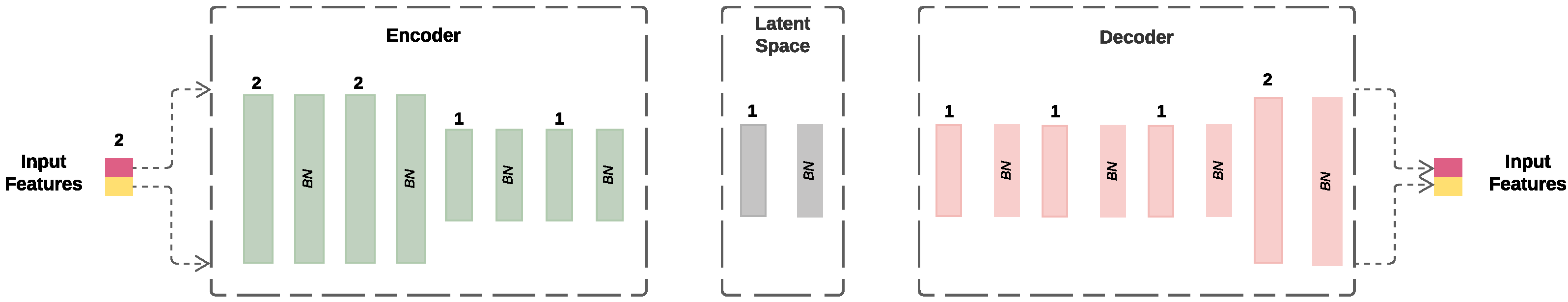
for each input instance, where higher reconstruction errors stand for a higher abnormality probability. As previously mentioned, the architecture we developed assumes
pairs as input and produces two output nodes which form a fully connected structure including a stack of layers for both stages. All intermediate hidden layers are activated using the ReLU function, contrasting with the output nodes which assumes a logistic function (all
and
values are normalized ∈[0, 1] as previously described). To address and reduce the internal covariate shift, which occurs when the input distribution of the training and test set differ but the output label distribution remains intact, we apply a Batch Normalization (BN) layer, discarding the need for dropout layers. In fact, batch normalization also normalizes the layer inputs for each batch of data that passes through it [
23]. The development of this network architecture, all its assumptions and decisions resulted from several trials, conducting during preliminary experiments using older screw tightening data. Each experiment was conducted by imposing one bottleneck layer with 1 hidden node and a varying range of additional hidden layers. The best performing architecture was achieved when the AE was composed of 20 layers (input,
BN, and output layers) as shown in
Figure 4. Additionally, all models were trained using the Adam optimization algorithm (which proved to be slightly better than SGD in our test case), using the previously described loss function (MAE), a total of 100 epochs and early stopping (with 5% of the training data being used as the validation set).
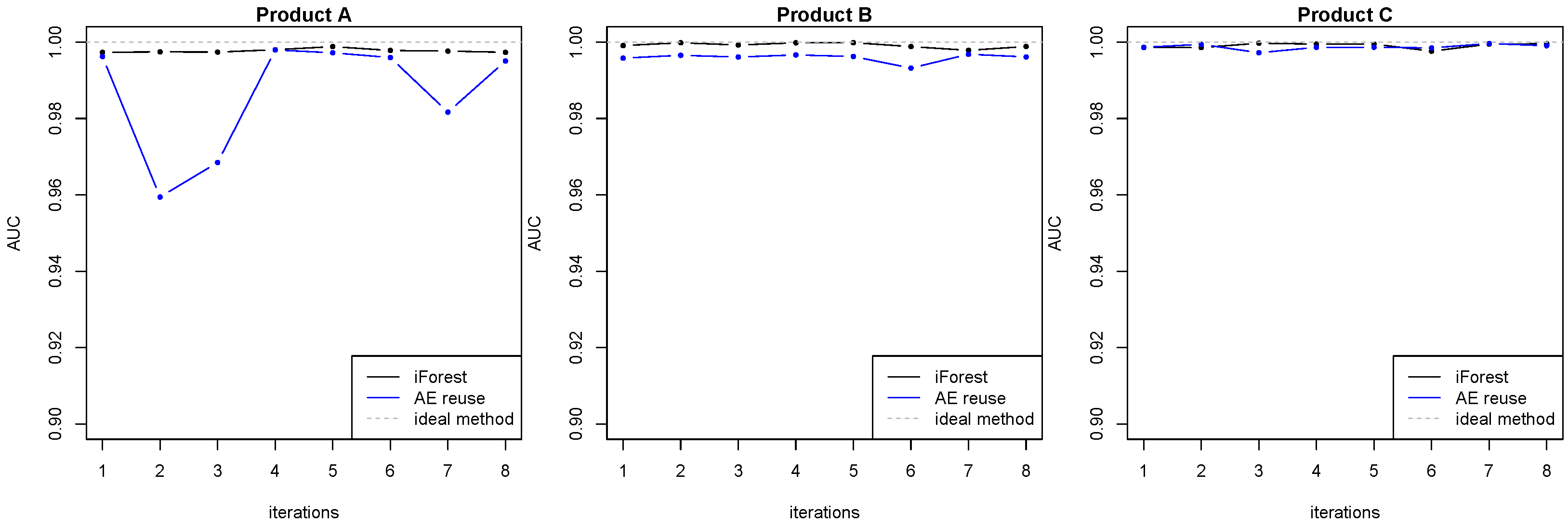
As explained in
Section 2, the AE model can be adapted to dynamic environments when there are frequent data updates. In [
24], two neural network learning modes were compared: reset and reuse. When new data arrives and the neural network is retrained, the former assumes a random weight initialization, while the latter uses the previously trained weights as the initial set of weights.
3.4. Evaluation
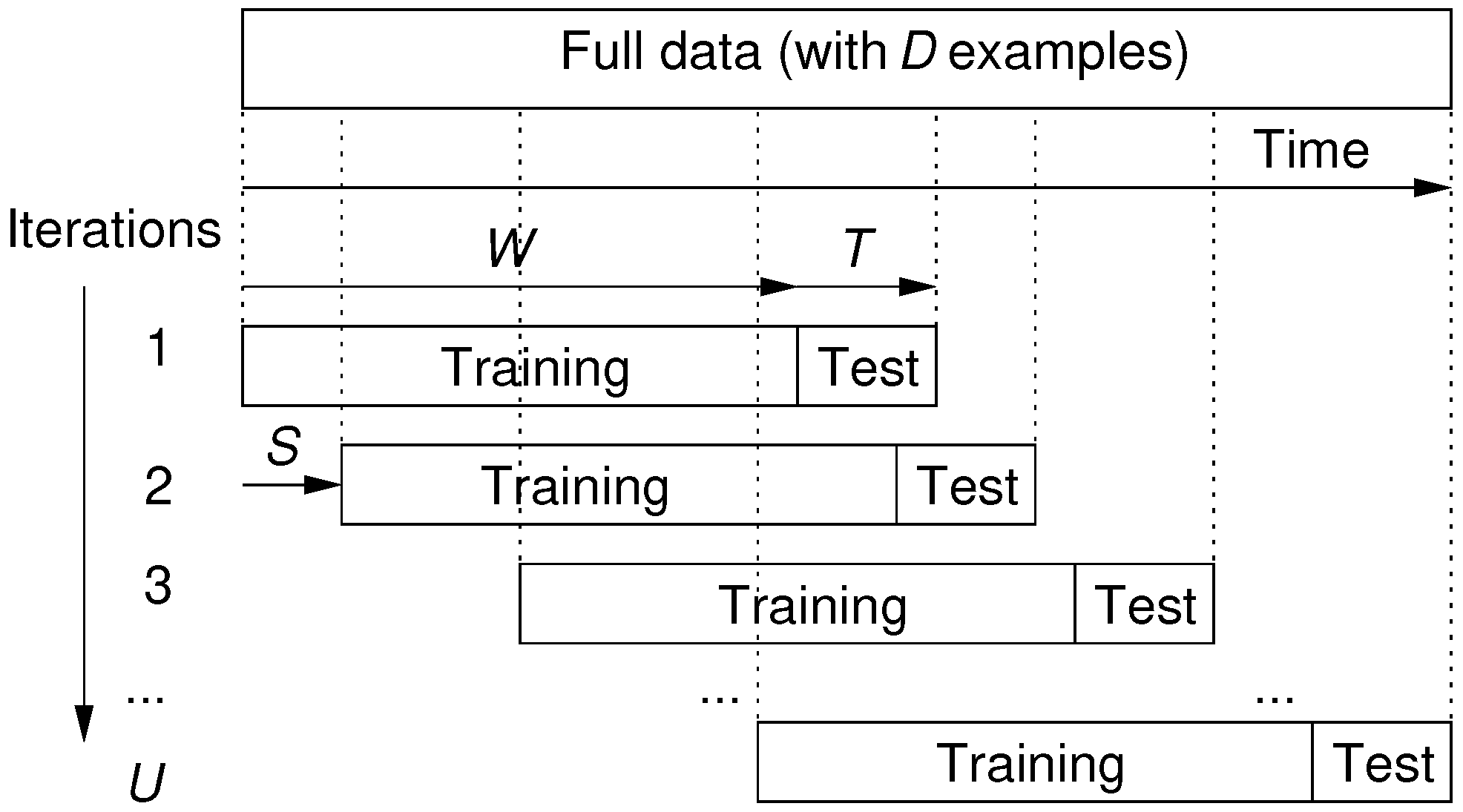
With the goal of assessing a robust performance, for both IForest and AE methods we assumed the realistic rolling window procedure [
24,
25]. This procedure includes a fixed size window for the training (
W) and test (
T) data and that rolls over time by using a jumping step (of size
S), thus generating several training and testing model iterations (
Figure 5). At the end, there are a total of
iterations, where
D denotes is the total number of screw cycles available in the analyzed data. During each rolling window iteration execution, only the training data is used to fit the ML model, thus the test set is considered as “unseen” data, meaning that it is only used for anomaly detection performance evaluation purposes. The goal of this evaluation is to realistically measure the behavior of the anomaly detection methods through time, assuming a continuous model retraining usage. Using the most recently collected data (regarding the three analyzed products), and after consulting the manufacturing experts, we assume a total of
standard rolling window train and test iterations by fixing the following values: Product A–
W = 6809,
T = 851, and
S = 106; Product B–
W = 36,529,
T = 4566, and
S = 570; Product C–
W = 10,530,
T = 1316, and
S = 164 (all values related to numbers of screw fastening processes). We particularly note that these values are much higher than the ones employed in our previous work [
1]. This occurs because previously we have collected only two days of screw industrial data, while our product datasets (presented in this work) have a substantially higher number of data records (67,337 fastening cycles related with two months).
To evaluate the anomaly detection performance, we adopt the Receiver operating characteristic (ROC) curve [
16], which produces a visual representation of the ability of a binary classifier to distinguish between normal and anomalous data as its discrimination threshold varies. In the case of both the standard and static training rolling window procedures, the ROC curves are computed by using the target labels and the anomaly scores (
) for the
T tightening test examples of each rolling window iteration. The overall discrimination ability is then measured by the Area Under the Curve (
AUC =
) and the Equal Error Rate (EER). As argued in [
26], the AUC measure has several advantages. For instance, the measurement of quality is is unaffected by balancing issues in the dataset (as previously explained, our datasets are highly unbalanced). Additionally, interpreting its results is fairly easy and can be categorized as follows: 50%—performance of a random classifier; 60%—reasonable; 70%—good; 80%—very good; 90%—excellent; and 100%—perfect. The EER is used to predetermine the threshold value for which the false acceptance rate and false rejection rate is equal [
27]. Under this criterion, the lower the value, the more accurate the classification. Given that multiple AUC and EER values are generated for each rolling window iteration, the experimentation results are aggregated by computing their median values and using the Wilcoxon non-parametric statistic test [
28] to check whether the paired median differences are statistically significant.
All experiments were executed on a M1 Pro processor with integrated GPU. For each ML model, we collected the computational effort, measured in terms of the rolling window average preprocessing, training, and testing (inference) time (all in seconds s), per anomaly detection method. This is of particular interest to the manufacturing experts that need to deploy the developed systems in an industrial context with near real-time requirements.


