Article

Hierarchical Control for DC Microgrids Using an Exact Feedback Controller with Integral Action

by
Oscar Danilo Montoya
1,2,*,
Federico Martin Serra
3 and
Alexander Molina-Cabrera
4
1
Facultad de Ingeniería, Universidad Distrital Francisco José de Caldas, Bogotá 110231, Colombia
2
Laboratorio Inteligente de Energía, Facultad de Ingeniería, Universidad Tecnológica de Bolívar, Cartagena 131001, Colombia
3
Laboratorio de Control Automático (LCA), Facultad de Ingeniería y Ciencias Agropecuarias, Universidad Nacional de San Luis—CONICET, Villa Mercedes, San Luis 5730, Argentina
4
Facultad de Ingeniería, Universidad Tecnológica de Pereira, Pereira 660003, Colombia
*
Author to whom correspondence should be addressed.
Computers 2022, 11(2), 22; https://doi.org/10.3390/computers11020022
Submission received: 4 January 2022 / Revised: 26 January 2022 / Accepted: 3 February 2022 / Published: 6 February 2022
(This article belongs to the Special Issue Computing, Electrical and Industrial Systems 2022)

Abstract

:
This paper addresses the problem of the optimal stabilization of DC microgrids using a hierarchical control design. A recursive optimal power flow formulation is proposed in the tertiary stage that ensures the global optimum finding due to the convexity of the proposed quadratic optimization model in determining the equilibrium operative point of the DC microgrid as a function of the demand and generation inputs. An exact feedback controller with integral action is applied in the primary and secondary controller layers, which ensures asymptotic stability in the sense of Lyapunov for the voltage variables. The dynamical model of the network is obtained in a set of reduced nodes that only includes constant power terminals interfaced through power electronic converters. This reduced model is obtained by applying Kron’s reduction to the linear loads and step nodes in the DC grid. Numerical simulations in a DC microgrid with radial structure demonstrate the effectiveness and robustness of the proposed hierarchical controller in maintaining the stability of all the voltage profiles in the DC microgrid, independent of the load and generation variations.

1. Introduction

1.1. General Context

Electrical distribution networks with DC technologies have rapidly been incorporated in the current electric systems, mainly in high-voltage (transmission systems) and low-voltage (i.e., microgrids) applications [1,2]. The operation with DC technology has important advantages over conventional AC grids, such as reduced energy losses, better voltage profiles, and absence of reactive or frequency concepts, which allow for the easy control of these grids [3,4,5]. However, to make DC networks feasible, fundamental devices that allow interfacing of renewable energies, energy storage devices, controllable loads, and conventional AC grids are needed [6]. These devices are power electronic converters that can be either AC-DC or DC-DC [7,8]; nonetheless, independent of the nature of the power electronic interface, they are needed to implement efficient control methodologies to ensure the secure (i.e., stable) operation of the whole network [9]. Note that in the case of a DC microgrid, as presented in Figure 1, ensuring the secure operation is not enough to ensure the correct operation of each converter. Rather, a complete grid operation strategy is required for the entire microgrid, which is only possible with the application of a hierarchical controller [10], where the primary and secondary control layers ensure the correct operation of the converters and the third control layer is entrusted with defining the best grid operative point as a function of the generation and load behaviors [11,12].

1.2. Motivation

The recent advancements in DC networks and their high-efficiency levels (compared with AC microgrids) served as our source of motivation to further research in this area and to contribute to the topic of employing the hierarchical control design to microgrid applications, where multiple constant power terminals are interconnected through a DC distribution grid [13]. Hierarchical controllers are complex systems that are entrusted with the safe operation of an electrical system where different dynamics interact; essentially, a hierarchical controller can be considered as the brain of an electrical network, since it takes decisions based on optimization concepts and sends these decisions to each controllable device to execute these orders in the physical layer of the grid [14]. A general hiearchical controller for DC microgrids is depicted in Figure 2 [11].
Note that the hierarchical control design presented is only based on the measurements available in the controllable devices, which are sent to the centralized controller through a distributed communications network. Once the controller defines the references that must be applied into the converters, these are sent to them again using the same communication infrastructure [15]. It is worth mentioning that the usage of communication channels with adequate protocols is one of the most important aspects in the adequate performance of the smart controllers for electrical microgrids [16,17]. This is because they are responsible for transporting valuable information regarding the measurements and control signals; hence, when possible these communication networks must be constructed with redundant structure [18].

1.3. Review of the State of the Art

The extant literature in the field reveals multiple hierarchical controllers that have been proposed for the management of energy in DC networks. Some of these are presented and discussed below. Authors of [11] proposed a primary-secondary control design for DC microgrids based on the passivity properties of the dynamical model of the network. The authors proposed the application of the interconnection and damping passivity-based controller with a pure proportional gain. The proposed controller ensures asymptotic stability, and it uses a unique parameter to control the entire DC microgrid. Numerical results of the study are interesting; however, a comparison with classical controllers was not provided, and the DC microgrid was simplified and solved through a differential equation package that does not include the dynamic of the DC distribution lines by representing them with pure resistive effects. Montoya et al., in [15], proposed the improvement of the passivity-based controller presented in [11] with the inclusion of an integral gain to reduce possible steady-state errors introduced by unmodeled dynamics. Numerical results in a multi-terminal high-voltage DC (i.e., MT-HVDC) grid confirm the effectiveness of including the integral action with respect to the pure proportional approach stated in [11]. Authors of [13] proposed the application of the inverse optimal control (IOC) design to stabilize MT-HVDC networks. The main contribution of these authors, as in [15], was the inclusion of an integral gain, thus maintaining the asymptotic stability properties of the studied controller. Numerical comparisons with passivity-based controllers show that the proposed IOC design can have less oscillations with minimum settling times than the passivity designs. Ashourloo et al., in [19], proposed the stabilization of a DC microgrid using the active damping method. The tuning of the parameters of the controller was carried out using the particle swarm optimization method. Numerical results show that in the proposed approach the constant power terminals change their power consumptions and the voltage profile remains stable with asymptotic convergence. However, the authors do not compare their proposal with other control methodologies, which makes it difficult to measure the real efficiency of the proposed active damping controller. Grisales et al., in [20], proposes an energy management system for DC microgrids based on photovoltaic generation, energy storage systems, and constant power loads. The controller design ensures asymptotic convergence to the desired voltage profile through the application of the sliding control method. Numerical results ensured that the maximum power point tracking of the photovoltaic generation is always reached using the battery to compensate the load power requirements; nonetheless, no comparisons with other control techniques were provided by the authors of this study.
It is important to mention that most of the reports about control applications focus on a particular application with reduced number of converters [21]. Thus, the control design using hierarchical controllers that allow stabilizing DC networks to their voltage references using optimization in the tertiary control is an area that requires urgent developments since few studies are available in the existing literature for this research field.

1.4. Contribution and Scope

Based on the review of the state of the art presented in the previous section, the main contributions of the present research are listed below:
  • The global stabilization of the voltage profiles in a DC microgrid by using an exact feedback controller design with integral gain. This controller helps to ensure asymptotic stability in the sense of Lyapunov during closed-loop operation. The main advantage of this control design is that the voltage variables are stabilized in their references in a settling time that does not exceed 10 ms.
  • The usage of a quadratic convex approximation to solve the optimal power flow problem in the tertiary control stage. This optimal power flow formulation has the main advantage of ensuring the global optimum finding convergence owing to the convexity of the solution space regarding the power flow equations since these are recursive linearized through a Taylor’s series approximation.
Note that the hierarchical controller design using the quadratic convex power flow in the tertiary control stage, with the exact feedback control design added in the primary-secondary control stage, has not previously been reported in the specialized literature. This was identified as an opportunity for research, and the present paper aims to contribute to this end.
It is worth emphasizing that the proposed hierarchical controller assumes a centralized communication system where all the measurements in the power electronic converters, i.e., voltage and currents, are available. In addition, it is assumed that the power injections in renewable energy sources and the expected demand in constant power loads are provided to the optimal power flow problem by a prediction system, which implies that they are considered exogenous inputs, which are non-controllable in the current study.

1.5. Organization of the Document
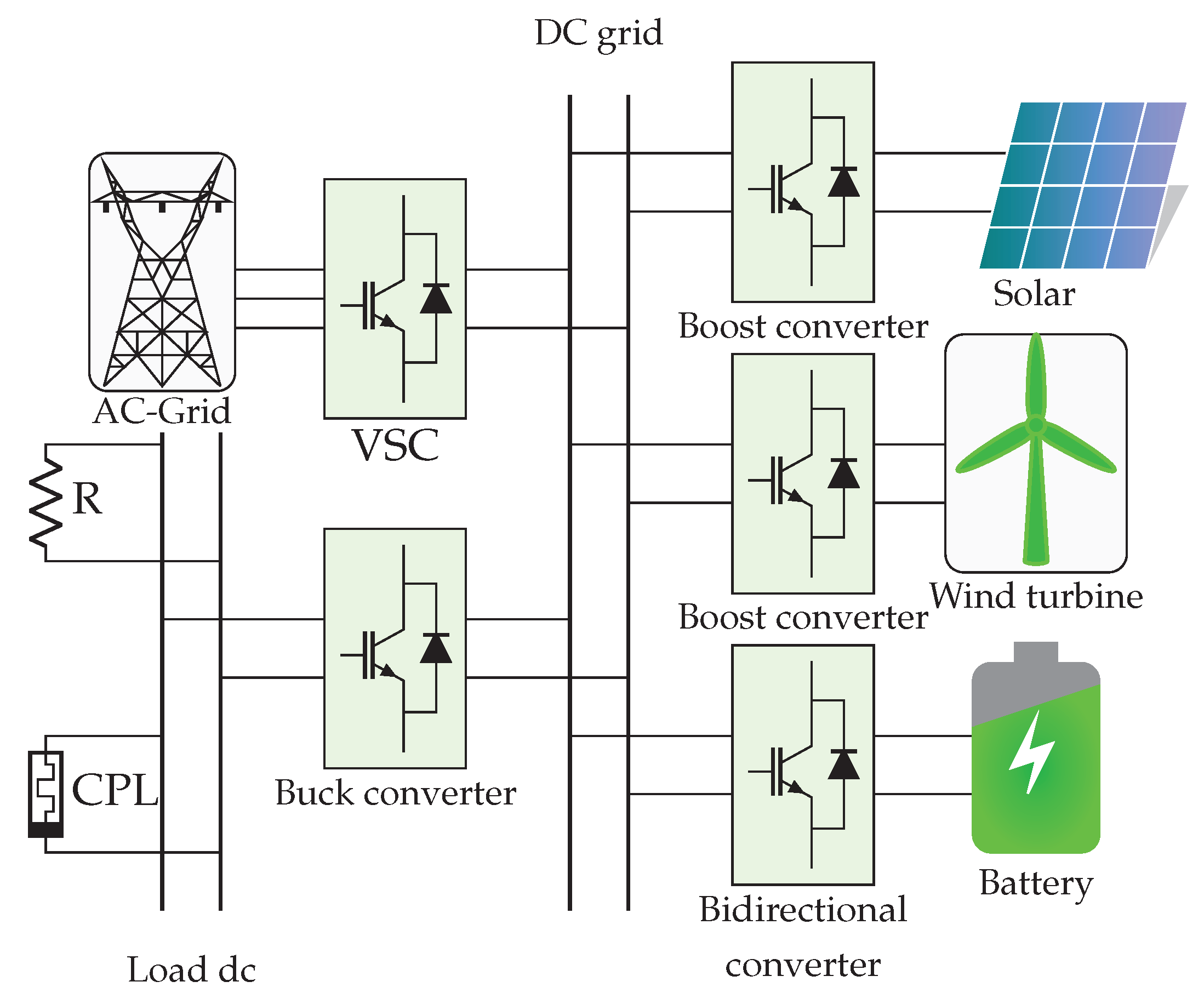
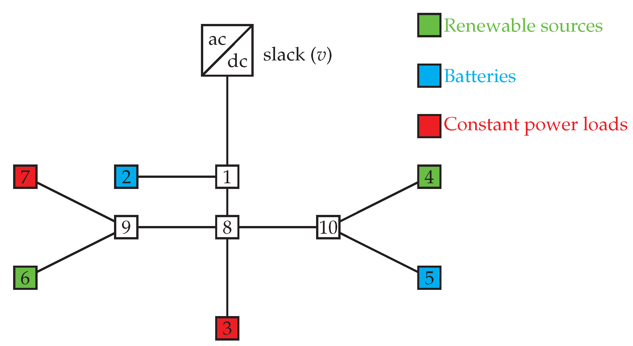
The remainder of this document is structured as follows: Section 2 presents the dynamical model of a DC microgrid with multiple constant power terminals. Section 3 presents the design of the exact feedback controller with integral action, and it also provides the proof of asymptotic convergence. Section 4 shows the optimization methodology to determine the voltage references through the solution of a quadratic convex optimal power flow model. Section 5 summarizes the main aspects of the proposed hierarchical controller through a pseudo-code. Section 6 presents the main simulations in a 10-bus DC microgrid and compares the exact feedback controllers with nonlinear controllers based on passivity and inverse optimal control theory. Finally, Section 7 presents the main conclusions derived from the present study as well as some recommendations for future research.

2. Grid Modeling

The electrical representation of a DC microgrid can be made by considering that the power electronic converters that are interfaced with the constant power terminals can operate as current-controlled sources [13]. Let us consider a general representation for a general k node in a DC microgrid, as illustrated in Figure 3 [15].
In Figure 3, c k represents the output capacitance of the converter that interfaces the constant power terminal, which absorbs or injects the power p k , g k is a possible linear load connected at node k, v k is the state variable relating to the voltage behavior at the node k, and i k represents the net injected current to the DC microgrid [11]. If Kirchhoff’s first law is applied to the node k, then the following first-order nonlinear differential equation is obtained [11]:
c k d d t v k = p k v k g k v k i k .
In the case of a microgrid with n nodes and s constant power terminals ( s < n ), it is possible to represent the net power injections/absorptions, in the s terminals, using Kron’s reduction. A general DC grid can be represented by the classical nodal admittance (conductance for DC networks) matrix equivalent in steady state conditions as follows:
I s I r G s s G s r G r s G r r V s V r ,
where G s s R s × s , G s r = G r s T R s × r , and  G r r R r × r are the conductance submatrices that relate nodes with power electronic converters and step-nodes or nodes with linear loads, I r R r × 1 is the current injected in step- and linear loads, and  V r R r × 1 corresponds to the voltages in these buses [11].
The application of Kron’s reduction is based on the following assumption: The total injected current in step-nodes and pure linear loads is null (i.e., I r = 0 ), since the effect of these linear loads can be completely included in the equivalent grid admittance matrix. With this consideration, the equivalent injected current in the constant power terminals takes the following form [15]:
I s = G s s G s r G r r 1 G r s V s = H s s V s .
Now, note that to generalize the representation of the s constant power terminals, the nonlinear differential equation in (1) can be rewritten in a matricial form as presented below:
C s V ˙ s = diag 1 V s P s G s V s I s ,
where C s is a positive definite diagonal matrix that contains all the capacitive effects in the constant power terminals; V s is the vector that contains all the voltage profile in the reduced set of nodes s; P s is the vector that contains all the constant power consumptions/absorptions in the constant power terminals; and G s is a constant diagonal semidefinite matrix that contains all the linear loads connected in parallel in the constant power terminals. Note that diag 1 V s is a positive diagonal definite matrix that contains all the inverse voltages of the reduced set of nodes s.
To obtain the general grid equivalent dynamic model that represents the behavior of the voltage profiles in the set of nodes s, (2) is substituted in (4), taking into account that J s s = G s + H s s :
C s V ˙ s = diag 1 V s P s J s s V s .
It is worth emphasizing that (5) corresponds to a set of nonlinear differential equations that defines the voltage behavior of the DC microgrid as a function of the amount of constant power injection/absorption in the constant power terminals, which are the control variables of this nonlinear model.
To apply the exact feedback control design to the dynamical system (5), let us consider the representation of this system with the state variables x as V s and the control input u as P s . These definitions allow representing (5) as follows:
C s x ˙ = diag 1 x u J s s x .

3. Exact Feedback Controller Design

The exact feedback nonlinear control design is a well-known control technique for nonlinear dynamical systems that has the ability to ensure asymptotic stability in the sense of Lyapunov from a particular set of dynamical models, which includes electrical and mechanical systems [22,23]. Note that using the general dynamical structure in (6), it is possible to define the exact feedback controller including an integral action as follows:
u = diag x J s s x 🟉 K p x ˜ + K i y ,
y ˙ = x ˜ ,
where x 🟉 is the equilibrium point of the dynamical system (i.e., the desired operative point); x ˜ is the error vector that measures the difference between the current value of the state variables and their reference point, i.e., x ˜ = x x 🟉 ; y is the integral of the error vector; and K p and K i are positive definite symmetric matrices related with the proportional and integral control gains respectively.
To ensure that the control law (7) and (8) have asymptotic convergence of the state variables to the reference point, let us consider the following candidate Lyapunov function:
V x ˜ = 1 2 x ˜ C s x ˜ + 1 2 y K i y ,
which fulfills the first two Lyapunov stability conditions, i.e., V x ˜ > 0 x x 🟉 and V x ˜ = 0 x = x 🟉 . Now, taking the time derivative of this function considering that x ˙ = x ˜ ˙ , since x 🟉 is a constant equilibrium point, we obtain the following result:
V ˙ x ˜ = x ˜ C s x ˙ + y K i y ˙ , = x ˜ diag 1 x u J s s x y K i x ˜ = x ˜ J s s x 🟉 K p x ˜ + K i y J s s x y K i x ˜ , = x ˜ J s s x ˜ K p x ˜ + K i y y K i x ˜ , V ˙ x ˜ = x ˜ J s s + K p x ˜ 0 .
Note that to obtain (10), the fact that y K i x ˜ = x ˜ K i y is considered, since the integral gain matrix is symmetric. In addition, the result in (10) shows that the state variable converges asymptotically to the desired operative point, as demonstrated in [24]. Now, the main challenge in the hierarchical control of a DC microgrid is to determine the desired reference point. This calculation will be presented in the next section.

4. Equilibrium Point Calculation

To determine the equilibrium point, where the state variables x must be stabilized, it is necessary to solve the set of nonlinear equations that results when x ˙ = 0 in (6), i.e.,
diag 1 x u J s s x = 0 , u = diag x J s s x .
This set of equations is popularly known in the literature as the power flow problem for DC networks [25]. However, in the case of hierarchical control, the tertiary stage (optimization stage) is entrusted with determining the best set of x 🟉 that optimizes some performance indicator for the DC grid. This indicator can be technical or economical; here, we adopt the minimization of the total grid losses for a particular injection/absorption in the constant power terminals. The equivalent optimization model that must be solved corresponds to the optimal power flow presented below:
Obj . Func . min P loss = x J s s x , Subject to : u = P s g P s d = diag ( x ) J s s x , P s g , min P s g P s g , max , x min x x max ,
where P s g R n × 1 is the vector that contains the constant power generations; P s d R n × 1 is the vector that contains all the constant power demands; x min R n × 1 and x max R n × 1 are the vectors with the minimum and maximum voltage regulation bounds of the network respectively; and P loss is the objective function value associated with the grid power losses.
To solve the nonlinear non-convex optimization model (12) it is possible to use semidefinite programming [26] or second-order cone programming [23]. However, even if these methodologies ensure the global optimum finding, they increase the number of variables in s 2 , adding to the impracticality of their use in large-scale applications. For this reason, here we use a recursive solution that maintains the number of decision variables constant at each iteration. Further, it converts the quadratic nonlinear optimization model (12) into a quadratic programming model with linear constraints. The recursive power optimal power flow solution takes the following form [27]:
Obj . Func . min P loss = x J s s x , Subject to : u = P s g P s d = diag ( x 0 ) J s s x + diag ( x ) J s s x 0 diag ( x 0 ) J s s x 0 , P s g , min P s g P s g , max , x min x x max ,
where x 0 represents the initialization of the voltages at the first iteration. Note that the convergence of the recursive optimal power flow in (13) is reached when the maximum error between x t + 1 and x t is less than or equal to a desired tolerance ε , i.e.,
max x t + 1 x t ε .

5. Hierarchical Proposed Controller

The proposed hierarchical controller works in the primary-secondary stage with the exact feedback controller, which is entrusted with carrying all the state variables (voltages in the reduced set of nodes s) to their desired values x 🟉 . To do so, the control diagram depicted in Figure 4 is used for each power electronic interface [15].
Algorithm 1 is executed to send the control signal for each constant power terminal. Note that h 0 represents the starting time when the proposed hierarchical controller starts to optimally stabilize the DC microgrid.
 Algorithm 1: Hierarchical control design for stabilizing DC microgrids.
Data: Define DC grid topology and read the available power generation and consumptions.
e = 1;
for h h 0 do
Computers 11 00022 i001
It must be emphasized that the proposed hierarchical controller in Algorithm 1 is a centralized controller since its implementation requires that all the voltages and powers are available to generate the set of control signals to all the converters, as presented in Figure 4.

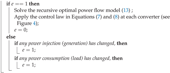
6. Numerical Validation

All simulations were carried out in MATLAB using its 2021b version on a PC with an AMD Ryzen 7 3700 2.3-GHz processor and 16.0 GB RAM, running on a 64-bit version of Microsoft Windows 10 Single Language. The electrical network was implemented with the help of the Simulink/Simscape environment. All the electrical values at the constant power terminals were measured with voltage and current measures, which were compacted and sent to the centralized controller. In addition, the exact feedback controller was implemented used MATLAB functions. All the simulations were carried in the discrete domain using a processing time of 1 μ s.
To demonstrate the effectiveness and robustness of the proposed hierarchical controller design, a DC microgrid composed of ten nodes is considered, which includes the slack source, two batteries, two renewable generators, and two constant power loads. The electrical configuration of this grid is depicted in Figure 5. The slack bus is operated with 48 V for this test feeder.
The electrical parameters associated with the resistances and inductances of the distribution lines for the 10-bus DC microgrid are listed in Table 1.
For the constant power terminals, i.e., nodes 1 to 7, the electrical parameters associated with the capacitances and the power injection/absorption are reported in Table 2. Note that the negative sign indicates that the node is absorbing power. Further, P i j represents the constant power value at node i in the period j.
Now, considering the information for each period of time listed in Table 2, the optimal power flow model (13) is solved to find the voltage reference for each period of analysis. The voltage behavior for each of the nodes in the set s is listed in Table 3.
To verify the results of the optimal power flow model (13) and to ensure that the solution of the voltage profiles is indeed the optimal, the classical power flow method based on the Newton-Raphson method, as reported in [25], was used. Numerical results showed that the error between the results of the two methods was less than 1 × 10 10 .

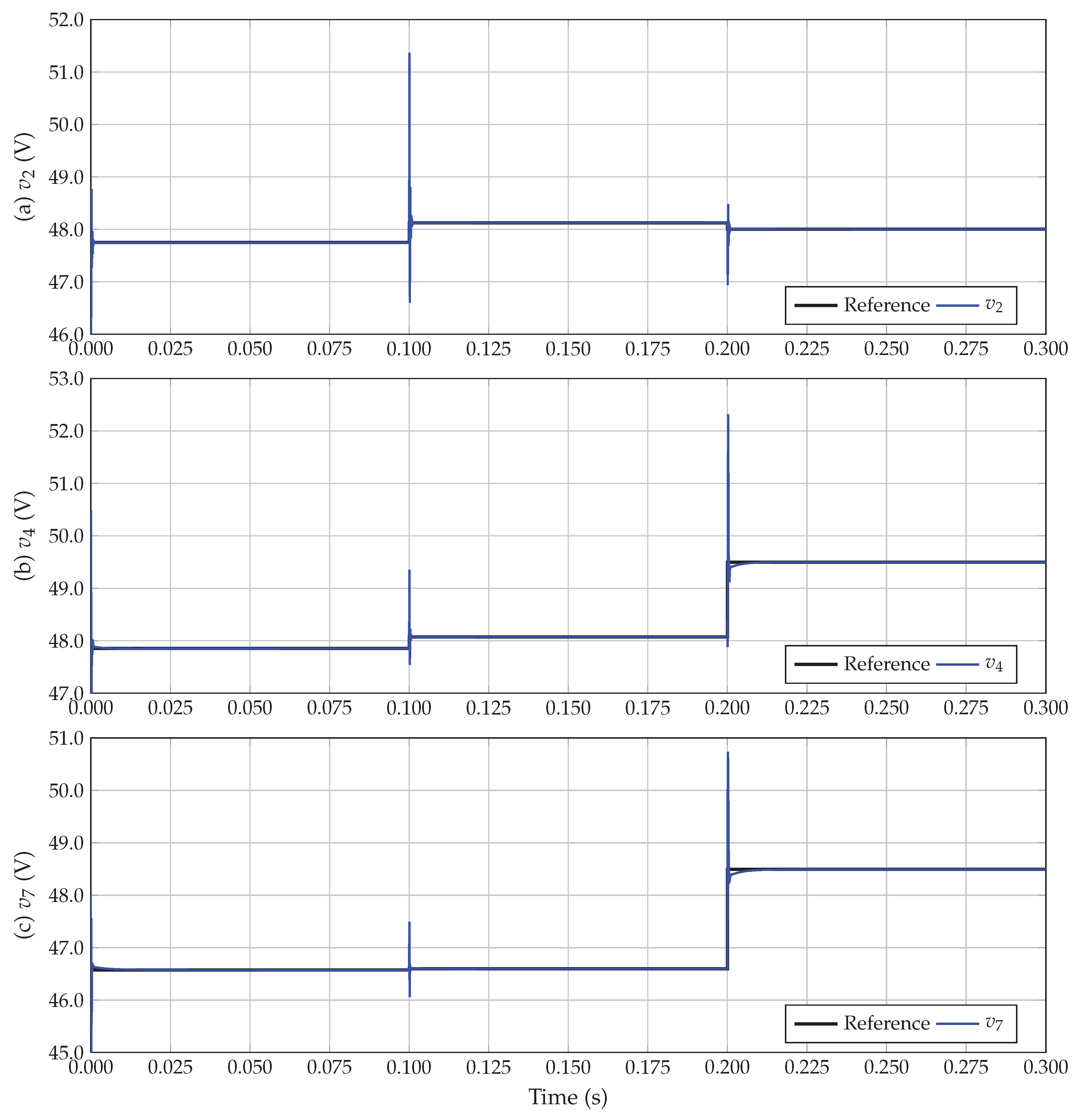
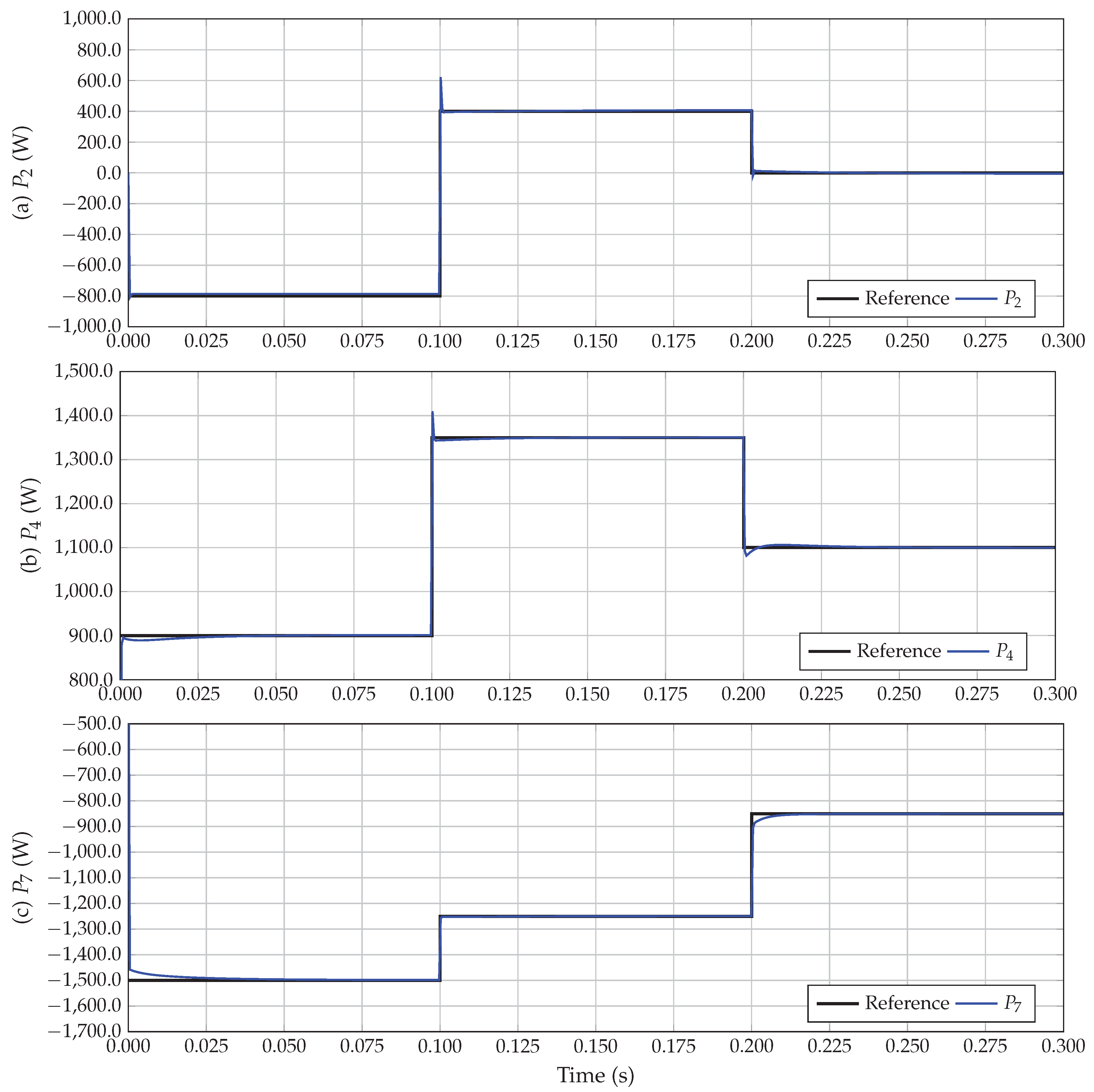
6.1. Tracking References

In this simulation scenario we evaluate the effectiveness of the proposed exact feedback controller with integral action to track the equilibrium points provided by the optimal power flow solutions. The voltage behavior at nodes 2, 4, and 7 are depicted in Figure 6. These nodes are selected since each one of them has a different device connected to them: a battery package at node 2, a renewable energy resource at node 4, and a constant power demand at node 7.
The following observations can be noted from the output voltage behaviors presented in Figure 6:
Each of the voltage profiles of the network reaches its reference value within a settling time less than 10 ms, which is quite fast, considering that the constant power terminals vary their behavior every 100 ms.
The state variables exhibit an oscillatory behavior around their reference. In the case of node 2, the maximum overshot was about 51.38 V when the simulation time was 100 ms, which amounts to about 3.30 V with respect to the desired voltage reference, which is a typical tolerable voltage variation in a DC microgrid. The maximum values at nodes 4 and 7 were 52.46 V and 50.76 V respectively.
The numerical results in Figure 6 were obtained when the proportional and integral gain matrices, i.e., K p and K i , were set as 5 J s s and 5000 J s s respectively.
Figure 7 presents the power output at terminals 2, 4, and 7 when the voltage and current measurements are connected to the point where the converter is coupled with the DC grid (see current i k in Figure 4).
The following observations can be highlighted from the power behavior at the constant power terminals: (i) The battery connected at node 2 absorbs 800 W during the first 100 ms, following which it provides about 400 W of power to the grid in the time period between 100 s and 200 ms; the battery does not provide/absorb energy after 200 ms. These behaviors demonstrate that batteries can work as a demand, as a generator, or as a neutral device, depending on the grid requirements and the available energy stored in it; (ii) The constant power terminal 4 works as a generator since the power is positive in all the periods of time analyzed; and (iii) The constant power terminal in bus 7 is a constant power demand since in all the analyzed periods of time it only absorbs power from the grid.
However, the main result that can be extracted from Figure 7 is that in all of the cases once the voltages are stabilized around their references, then all of the power injections/absorptions in the constant power terminals reach their optimal values. This proves that the proposed hierarchical controller stabilizes the state variables of the network in an asymptotic manner, as the theoretical development has affirmed.

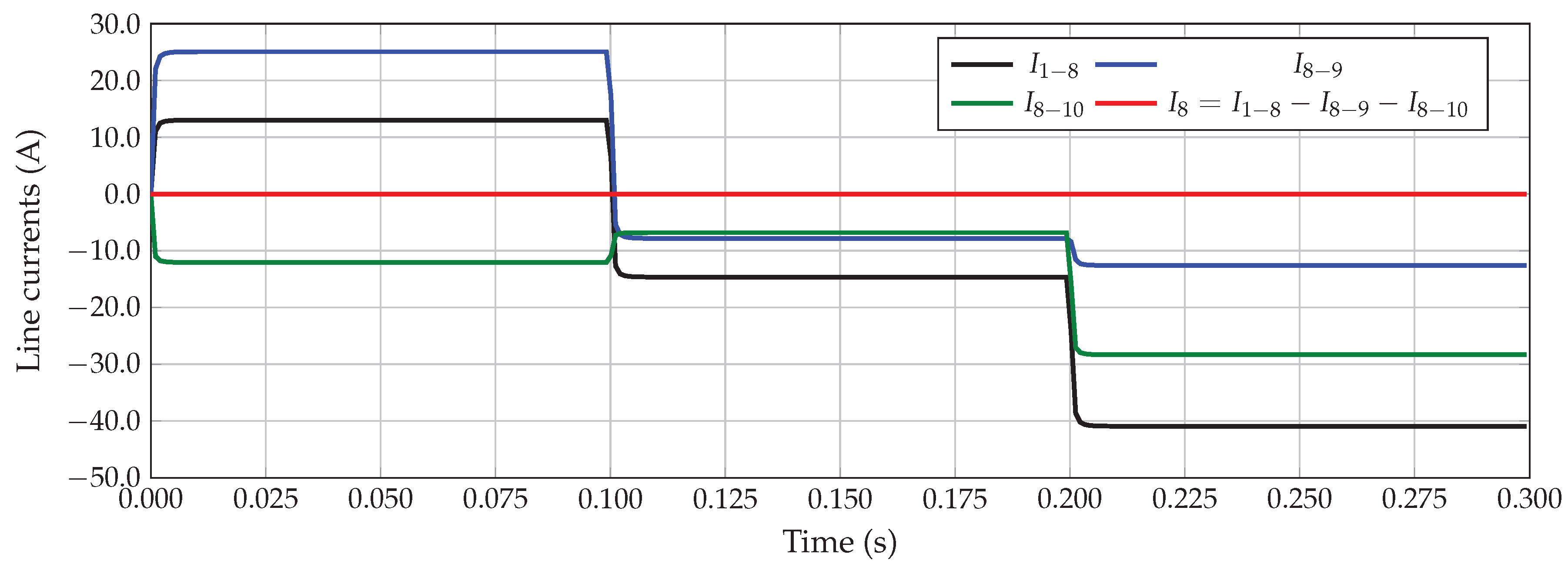
6.2. Current Behavior in a Step-Node

To demonstrate that the proposed controller ensures the correct operation of the whole DC microgrid, here, we select the step-node 8 to present the behavior of the currents in its adjacent lines as well as the total net current injection. The behavior of the currents in the lines that connects with the node 8 are depicted in Figure 8.
The behavior of the currents at node 8 shows that for each voltage reference in the constant power terminals the currents adjacent to this node change their behavior to maintain the power equilibrium in the whole DC microgrid. In addition, the main result in Figure 8 is the confirmation that the net injected current at this node, i.e., I 8 , is zero for all the periods of time, which implies that the net injected power at this node is also zero. This result is very important since during the controller design node 8 was reduced using Kron’s reduction; however, the operation of the complete microgrid is not affected by this reduction, which confirms the effectiveness of the proposed hierarchical control design to hold the DC network stable under load variations.

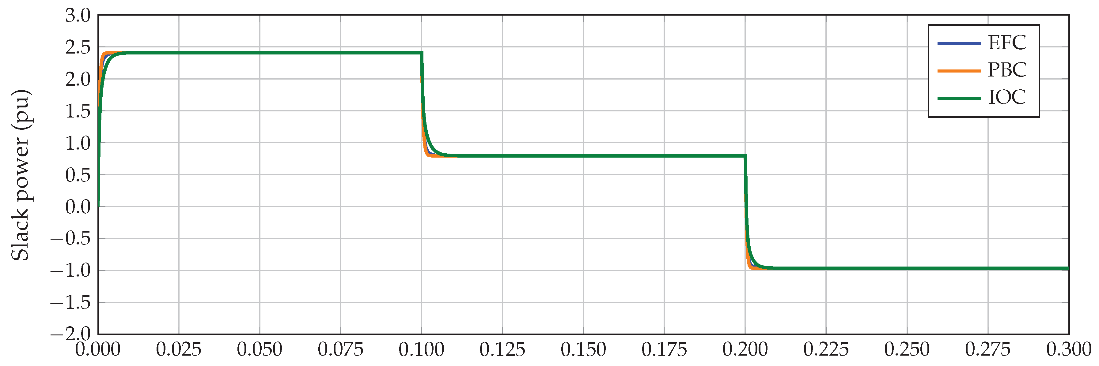
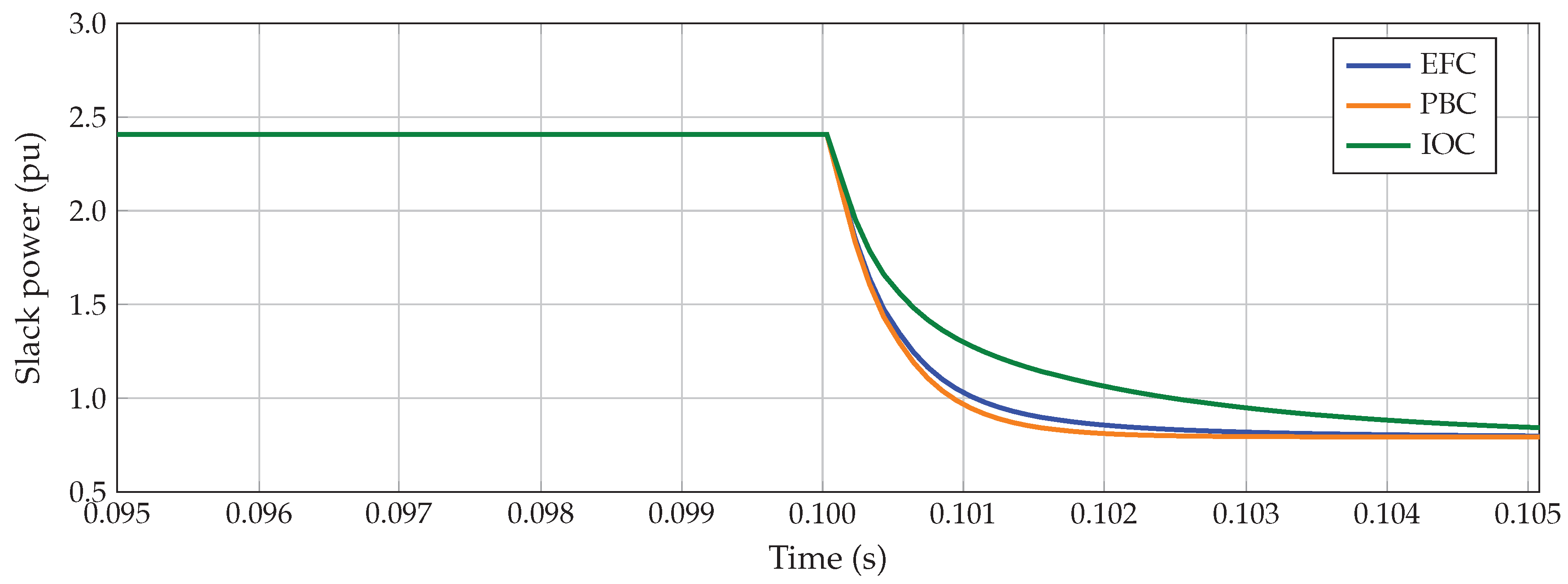
6.3. Comparison with Passivity and Inverse Optimal Controllers

To demonstrate that the proposed hierarchical control design based on the exact feedback controller (EFC) with integral action is more efficient in stabilizing the grid when compared with nonlinear controllers from the same family, the following simulation is developed. From 0 ms to 100 ms, node 6 maintained a reference of 46 V; however, after 100 ms, this node reaches a reference of 50 V. Note that the voltages in all the other nodes remain consistent with the reference reported in Table 3. Figure 9 presents a magnified view of the area between 95 ms and 115 ms to show the effect of each controller on the voltage profile at node 6.
The formulation of the passivity-based controller (PBC) can be found in [11], which takes the form presented in (15), while the inverse optimal controller (IOC) was reported in [13] with the form defined in (16):
u PBC = diag x J s s x μ J s s x ˜ ,
u IOC = 1 2 diag 1 x γ J s s x ˜ + δ J s s y , y ˙ = x ˜ ,
where μ and γ are set as 5, and δ is equal to 5000. These value are selected to ensure that all the controllers have a comparable performance.
Voltage curves in Figure 9 show that (i) the proposed EFC and the PBC have similar performances regarding voltage peak and settling time; this occurs because the PBC is a particular case of the proposed controller without integral action, as can be seen when the proposed controller in (7) is compared with the passivity-based approach in (15); and (ii) the IOC does not present an overshoot as in the cases of the PBC and EFC; however, its settling time is greater than 5 ms in the studied case. This is attributable to the controller form since this case does not include the effect of the conductance matrix and the state variables or the desired reference in the control formulation (16), as in the cases of the passivity-based and exact feedback controllers. In addition, the IOC works with the inverse of the voltage profiles, while the other two controllers use these voltages in a proportional manner, which can affect the final performance of the controller.
It is important to emphasize that all the compared controllers can be considered adequately capable of stabilizing the state variables (i.e., voltages) in DC microgrids. Further, its numerical performance will also be the same if a specialized optimization technique is applied to tune all the controller parameters [13], since all of these controllers are from the family of the Lyapunov-based control designs.
An additional comparison to show the effectiveness of the studied controllers in maintaining stable power flow is presented in Figure 10, where the output power in the slack node is presented for each one of the studied controllers.
The behavior of the power output in the slack source for the different controller designs show that all the controllers effectively stabilize the power flow generation in the slack node, which clearly depends on the constant power terminals and their behavior during each period of time. However, we can note that the behavior of all the controllers is very similar to a first-order system, with the proposed EFC and the PBC having control approaches with better settling times. These settling times can be better observed in the magnified view presented in Figure 11, which shows that the EFC and the PBC takes about 5 ms to reach a stable behavior, similar to the behavior explained for voltages in Figure 9.

6.4. General Commentaries

The proposed hierarchical controller design based on the application of the recursive optimal power flow solution in the tertiary stage and the exact feedback control design in the primary-secondary stages can have the following limitations:
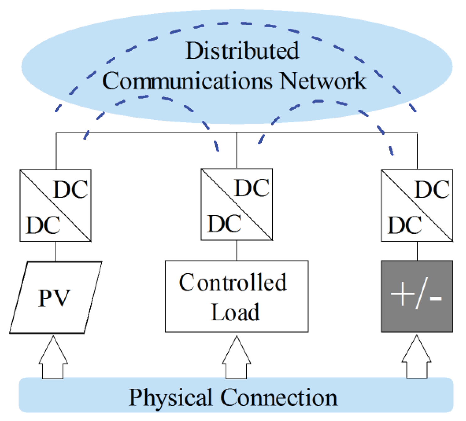
The requirement of a complete communication structure that connects all the controllable constant power terminals and the slack source, which permits obtaining all the information so as to solve the recursive power flow problem using a centralized computation center. These information will be sent to the local controllers using the same communication system. For this reason, it is recommended to have a redundant communication system to ensure the correct operation of the proposed hierarchical controller.
The proposed hierarchical controller design assumes that the local current controllers in the power electronic converters that interface the loads are faster than the centralized controller since they can help with the stabilization of the grid in the case of sudden load variations or grid topology changes, even if the tertiary controller has not updated all the reference signals.

7. Conclusions

The problem of the optimal stabilization of DC microgrids was addressed in this research from the perspective of the hierarchical control design. In the tertiary control stage, an optimal quadratic convex power flow formulation was employed to define the reference points for the voltage profiles; in the primary-secondary control stage, the application of the exact feedback controller design with integral action was proposed. The main advantage of this controller is that the asymptotic stability in the sense of Lyapunov was ensured taking advantage of the well-known proportional-integral gains.
Numerical simulation in a 10-bus DC microgrid with multiple constant power terminals demonstrated that the proposed hierarchical controller allowed the desired voltage reference to be reached with settling times less than 10 ms; in addition, the overshoots of the voltage variables after applying step references were less than 4 V for all the simulation cases. Furthermore, numerical comparisons with passivity-based and inverse optimal control designs confirmed the effectiveness of the proposed controller in stabilizing the voltage variables into their reference with asymptotic convergence and faster settling times.
The comparison of the output power in the slack source for the proposed EFC and for the comparative methods, i.e., the PBC and the IOC, showed that the behavior of this variable is similar to a first-order system, with the settling times for the EFC and the PBC being about 5 ms, while the IOC took more than 10 ms to stabilize the output power in the slack bus.
Future studies can develop the following research trajectories: (i) The complete dynamics of each DC-DC converter that interface renewable energy resources, energy storage devices, and controlled power loads can be included in the proposed hierarchical controller; (ii) The proposed controller can be extended to AC microgrids with constant power terminals; and (iii) The proposed hierarchical controller design can be validated for DC microgrids with an experimental platform.

Author Contributions

Conceptualization, methodology, software, and writing—review and editing, O.D.M., F.M.S. and A.M.-C. All authors have read and agreed to the published version of the manuscript.

Funding

This work was supported in part by the Centro de Investigación y Desarrollo Científico de la Universidad Distrital Francisco José de Caldas under grant 1643-12-2020 associated with the project: “Desarrollo de una metodología de optimización para la gestión óptima de recursos energéticos distribuidos en redes de distribución de energía eléctrica”.

Institutional Review Board Statement

Not applicable.

Informed Consent Statement

Not applicable.

Data Availability Statement

No new data were created or analyzed in this study. Data sharing is not applicable to this article.

Acknowledgments

This work has been derived from the doctoral research project: “Análisis, operación y control de convertidores para la integración de recursos energéticos distribuidos en redes eléctricas aisladas” presented by the student Oscar Danilo Montoya to the Doctoral program of the Engineering Faculty at Universidad Nacional de Rio Cuarto as a partial requirement for the PhD in Engineering Sciences.

Conflicts of Interest

The authors declare no conflict of interest.

References

  1. Rodriguez, P.; Rouzbehi, K. Multi-terminal DC grids: Challenges and prospects. J. Mod. Power Syst. Clean Energy 2017, 5, 515–523. [Google Scholar] [CrossRef] [Green Version]
  2. Simiyu, P.; Xin, A.; Bitew, G.T.; Shahzad, M.; Kunyu, W.; Tuan, L.K. Review of the DC voltage coordinated control strategies for multi-terminal VSC-MVDC distribution network. J. Eng. 2018, 2019, 1462–1468. [Google Scholar] [CrossRef]
  3. Garces, A. Uniqueness of the power flow solutions in low voltage direct current grids. Elect. Power Syst. Res. 2017, 151, 149–153. [Google Scholar] [CrossRef]
  4. Grisales-Noreña, L.F.; Garzón-Rivera, O.D.; Ocampo-Toro, J.A.; Ramos-Paja, C.A.; Rodriguez-Cabal, M.A. Metaheuristic Optimization Methods for Optimal Power Flow Analysis in DC Distribution Networks. Trans. Energy Syst. Eng. Appl. 2020, 1, 13–31. [Google Scholar] [CrossRef]
  5. Planas, E.; Andreu, J.; Gárate, J.I.; de Alegría, I.M.; Ibarra, E. AC and DC technology in microgrids: A review. Renew. Sustain. Energy Rev. 2015, 43, 726–749. [Google Scholar] [CrossRef]
  6. Savitha, K.P.; Kanakasabapathy, P. Multi-port DC-DC converter for DC microgrid applications. In Proceedings of the 2016 IEEE 6th International Conference on Power Systems (ICPS), New Delhi, India, 4–6 March 2016. [Google Scholar] [CrossRef]
  7. Singh, B.; Singh, B.; Chandra, A.; Al-Haddad, K.; Pandey, A.; Kothari, D. A Review of Three-Phase Improved Power Quality AC–DC Converters. IEEE Trans. Ind. Electron. 2004, 51, 641–660. [Google Scholar] [CrossRef]
  8. Mumtaz, F.; Yahaya, N.Z.; Meraj, S.T.; Singh, B.; Kannan, R.; Ibrahim, O. Review on non-isolated DC-DC converters and their control techniques for renewable energy applications. Ain Shams Eng. J. 2021, 12, 3747–3763. [Google Scholar] [CrossRef]
  9. Dragicevic, T.; Lu, X.; Vasquez, J.; Guerrero, J. DC Microgrids–Part I: A Review of Control Strategies and Stabilization Techniques. IEEE Trans. Power Electron. 2015, 1. [Google Scholar] [CrossRef] [Green Version]
  10. Shafiee, Q.; Dragicevic, T.; Vasquez, J.C.; Guerrero, J.M. Hierarchical Control for Multiple DC-Microgrids Clusters. IEEE Trans. Energy Convers. 2014, 29, 922–933. [Google Scholar] [CrossRef] [Green Version]
  11. Murillo-Yarce, D.; Garcés-Ruiz, A.; Escobar-Mejía, A. Passivity-Based Control for DC-Microgrids with Constant Power Terminals in Island Mode Operation. Rev. Fac. Ing. Univ. Antioq. 2018, 86, 32–39. [Google Scholar] [CrossRef]
  12. Simiyu, P.; Xin, A.; Mouhammed, N.; Kunyu, W.; Gurti, J. Multi-terminal Medium Voltage DC Distribution Network Large-signal Stability Analysis. J. Elect. Eng. Technol. 2020, 15, 2099–2110. [Google Scholar] [CrossRef]
  13. Montoya, O.D.; Gil-González, W.; Serra, F.M.; Angelo, C.H.D.; Hernández, J.C. Global Optimal Stabilization of MT-HVDC Systems: Inverse Optimal Control Approach. Electronics 2021, 10, 2819. [Google Scholar] [CrossRef]
  14. Papadimitriou, C.; Zountouridou, E.; Hatziargyriou, N. Review of hierarchical control in DC microgrids. Elect. Power Syst. Res. 2015, 122, 159–167. [Google Scholar] [CrossRef]
  15. Montoya, O.D.; Gil-González, W.; Garces, A.; Serra, F.; Hernández, J.C. Stabilization of MT-HVDC grids via passivity-based control and convex optimization. Elect. Power Syst. Res. 2021, 196, 107273. [Google Scholar] [CrossRef]
  16. Tightiz, L.; Yang, H. A Comprehensive Review on IoT Protocols’ Features in Smart Grid Communication. Energies 2020, 13, 2762. [Google Scholar] [CrossRef]
  17. González, I.; Calderón, A.J.; Portalo, J.M. Innovative Multi-Layered Architecture for Heterogeneous Automation and Monitoring Systems: Application Case of a Photovoltaic Smart Microgrid. Sustainability 2021, 13, 2234. [Google Scholar] [CrossRef]
  18. Elmouatamid, A.; Ouladsine, R.; Bakhouya, M.; Kamoun, N.E.; Khaidar, M.; Zine-Dine, K. Review of Control and Energy Management Approaches in Micro-Grid Systems. Energies 2020, 14, 168. [Google Scholar] [CrossRef]
  19. Ashourloo, M.; Khorsandi, A.; Mokhtari, H. Stabilization of DC microgrids with constant-power loads by an active damping method. In Proceedings of the 4th Annual International Power Electronics, Drive Systems and Technologies Conference, Tehran, Iran, 13–14 February 2013. [Google Scholar] [CrossRef]
  20. Grisales-Noreña, L.F.; Ramos-Paja, C.A.; Gonzalez-Montoya, D.; Alcalá, G.; Hernandez-Escobedo, Q. Energy Management in PV Based Microgrids Designed for the Universidad Nacional de Colombia. Sustainability 2020, 12, 1219. [Google Scholar] [CrossRef] [Green Version]
  21. Kwasinski, A.; Onwuchekwa, C.N. Dynamic Behavior and Stabilization of DC Microgrids With Instantaneous Constant-Power Loads. IEEE Trans. Power Electron. 2011, 26, 822–834. [Google Scholar] [CrossRef]
  22. Cardim, R.; Teixeira, M.C.; AssunçÃo, E.; Covacic, M.R. Design of state-derivative feedback controllers using a state feedback control design. IFAC Proc. Vol. 2007, 40, 22–27. [Google Scholar] [CrossRef]
  23. Li, P.; Wang, J.; Wu, F.; Li, H. Nonlinear controller based on state feedback linearization for series-compensated DFIG-based wind power plants to mitigate sub-synchronous control interaction. Int. Trans. Electric. Energy Syst. 2018, 29, e2682. [Google Scholar] [CrossRef] [Green Version]
  24. Cisneros, R.; Pirro, M.; Bergna, G.; Ortega, R.; Ippoliti, G.; Molinas, M. Global tracking passivity-based PI control of bilinear systems: Application to the interleaved boost and modular multilevel converters. Cont. Eng. Pract. 2015, 43, 109–119. [Google Scholar] [CrossRef]
  25. Garces, A. On the Convergence of Newton’s Method in Power Flow Studies for DC Microgrids. IEEE Trans. Power Syst. 2018, 33, 5770–5777. [Google Scholar] [CrossRef] [Green Version]
  26. Davoodi, E.; Babaei, E.; Mohammadi-Ivatloo, B.; Shafie-Khah, M.; Catalao, J.P.S. Multiobjective Optimal Power Flow Using a Semidefinite Programming-Based Model. IEEE Syst. J. 2021, 15, 158–169. [Google Scholar] [CrossRef]
  27. Montoya, O.D.; Gil-González, W.; Garces, A. Sequential quadratic programming models for solving the OPF problem in DC grids. Elect. Power Syst. Res. 2019, 169, 18–23. [Google Scholar] [CrossRef]
Figure 1. Multiple constant power terminals interconnected into a DC microgrid.
Computers 11 00022 g001
Figure 2. General design of a hierarchical controller for DC microgrids.
Computers 11 00022 g002
Figure 3. Equivalent model for a DC constant power terminal.
Computers 11 00022 g003
Figure 4. Application of the exact feedback controller in the primary-secondary control stage for voltage stabilization in DC microgrids.
Computers 11 00022 g004
Figure 5. Electrical configuration of the 10-bus DC microgrid.
Computers 11 00022 g005
Figure 6. Comparison between the voltage references and the grid voltage outputs at some nodes of the 10-bus DC microgrid: (a) voltage at node 2, (b) voltage at node 4, and (c) voltage at node 7.
Computers 11 00022 g006
Figure 7. Power behavior at some grid terminals: (a) power at node 2, (b) power at node 4, and (c) power at node 7.
Computers 11 00022 g007
Figure 8. The behavior of the line currents adjacent to node 8 and the net injected current at this node.
Computers 11 00022 g008
Figure 9. Comparison of the controllers’ performance in reaching a voltage that corresponds with the reference value.
Computers 11 00022 g009
Figure 10. Comparative power output in the slack source for all the studied controllers.
Computers 11 00022 g010
Figure 11. Zoomed-in area between 95 ms and 105 ms for the slack power in the studied hierarchical controller design.
Computers 11 00022 g011
Table 1. Line parameters for the 10-bus DC microgrid.
Line R ij ( Ω ) L ij ( μ H)Line R ij ( Ω ) L ij ( μ H)
1–20.0158.4010–40.0237.40
1–80.02511.010–50.03012.0
8–30.0229.009–60.03512.8
8–90.02011.69–70.0157.60
8–100.0178.00
Table 2. Line parameters for the 10-bus DC microgrid.
Node i C i ( μ F) P i 1 (W) P i 2 (W) P i 3 (W)
1150000
2250−8004000
3150−1200−1500−1000
422090013501100
5250−500−750300
620010007501500
7100−1500−1250−850
Table 3. Voltage profiles of each of the nodes in the set s for each period of time.
Node i V i 1 (pu) V i 2 (pu) V i 3 (pu)
1111
20.9947642536265801.002597420075621
30.9732384156877590.9689700810035871.00092826199327
40.9969253918248771.0014961362450501.03114934372463
50.9812786826005660.9780549659276601.02431368520600
60.9955694473117690.9906468599241551.03767163982958
70.9702457666974650.9707629436426381.01023463026772
Publisher’s Note: MDPI stays neutral with regard to jurisdictional claims in published maps and institutional affiliations.

