Abstract
Communication networks are managed more and more by using artificial intelligence. Anomaly detection, network monitoring and user behaviour are areas where machine learning offers advantages over more traditional methods. However, computer power is increasingly becoming a limiting factor in machine learning tasks. The rise of quantum computers may be helpful here, especially where machine learning is one of the areas where quantum computers are expected to bring an advantage. This paper proposes and evaluates three approaches for using quantum machine learning for a specific task in mobile networks: indoor–outdoor detection. Where current quantum computers are still limited in scale, we show the potential the approaches have when larger systems become available.
1. Introduction
Fast and accurate detecting of the physical location of a mobile device and its user is crucial for many new smart services in the current mobile networks. This information can be used by mobile operators to optimise their network to provide better (perceived) quality to their customers. It helps, for example, in detecting low-coverage areas and improving indoor coverage. Additionally, the functionality of location-based services can be enhanced when the operator can better predict the position of the mobile user. Machine learning is an important candidate to provide this information. Machine learning-based models then learn to classify the environment the mobile device is in. This could be a simple indoor or outdoor classification, however, a more complex classification is also possible where a distinction is made between, e.g., offices, shops, transportation and residential areas. The overview paper of [1] shows the huge variety in techniques: K-nearest neighbour, random forest, decision tree, logistic regression, support vector machine, naive Bayes and neural networks (NNs). If we look at the combination of the techniques in combination with the used data, we can give the following overview:
- Random forest and AdaBoost classifiers that use mobile device sensor data to classify the environment [2];
- Support vector machine (SVM) and deep learning (DL) techniques used in combination with a hybrid semi-supervised learning system to identify the indoor–outdoor environment using large and real collected 3rd Generation Partnership Project (3GPP) signal measurements [3];
- Deep learning, based on radio signals, time-related features and mobility indicators for a more complex environment classification, with multiple environments in [4].
- Ensemble learning schemes [5];
- Semi-supervised learning algorithm [6];
- Ensemble model based on stacking and filtering the detection results with a hidden Markov model [7].
For all these machine learning approaches, computing power is very important. More computing power leads to better results. In addition, the amount of available data is growing, which requires even more computing power. The end of Moore’s law for classical computing is approaching [8], however, a new paradigm is approaching rapidly: quantum computing. Quantum computers make use of quantum mechanical phenomena, such as superposition and entanglement, to perform operations on data. Superposition means that the system can be described by a linear combination of distinct quantum states. Entanglement means that measuring the state of a qubit is always correlated to the state of the qubit it is entangled with.
The quantum devices that are expected in the near feature to realise the first step in this demand for computing power are the so-called NISQ devices: noisy intermediate-scale quantum, involving a limited number of qubits that are not yet error-corrected nor noise-free. Machine learning is a prominent candidate to be among the first applications on these NISQ devices [9,10,11,12]. For a recent overview of quantum machine learning approaches, the reader is referred to Abohashima et al. [13]. One of the main benefits of quantum computers is the potential improvement in computational speed. Depending on the type of problem and algorithm, quantum algorithms can have a polynomial or exponential speed-up compared to classical algorithms. Biamonte et al. [14] indicate what the expected gain will be. For Bayesian inference [15], online perceptron [16] and reinforcement learning [9,17], quadratic speedup is expected. An exponential speed-up is expected for principal component analysis (PCA) [18], SVM [19] and least square fitting [20], compared to their classical counterparts.
There are, however, also other relevant benefits in the near future [10]. Quantum computers could possibly learn from less data, deal with more complex structures or could be better in coping with noisy data. In short, the three main benefits of quantum machine learning are (interpretation based on [21]):
- Improvements in run time: obtaining faster results;
- Learning capacity improvements: increase in the capacity of associative or content-addressable memories;
- Learning efficiency improvements: less training information or simpler models needed to produce the same results or more complex relations can be learned from the same data.
The exponential speed is mainly delivered by the use of the HHL [22] algorithm as part of the solution. This algorithm solves a system of linear equations very quickly. However, it is known that the fact that the data has to be encoded into the quantum state and that the output is in a quantum state will require a lot of effort to overcome. The author of [23] warns about the assumptions made by those quantum algorithms:
- They assume preloaded databases in quantum states, for example, using quantum RAM (QRAM);
- They assume data to be ‘relatively uniform’, meaning no big differences in value;
- They produce a quantum state as output, meaning this has to be translated efficiently to a meaningful result.
All are non-trivial to solve without losing the expected exponential gain.
In summary, we can say that machine learning is important for providing location information to mobile operators and that machine learning is an important application area for quantum computing, despite its current limitations. In this paper, we connect these two worlds by proposing quantum machine learning for indoor–outdoor classification. The main research question is ‘how can quantum computing, in the short term, support the demand for computing power that is needed by machine learning approaches in mobile networks?’. To the best of our knowledge, we are the first to propose the use of quantum machine learning in this area. Three approaches for quantum machine learning for this supervised machine learning problem are presented and evaluated on the current hardware. It is meant as starting point for further research. The growth of the number of qubits in the coming years will make real added value of quantum computers, quantum advantage, within reach in the next 5–10 years.
In the rest of this paper, first, a short introduction to quantum computing is provided in Section 2. Next, in Section 3, the data that were used in the analysis are generated. For this, a simple theoretical propagation model is used. Based on these data, three quantum machine learning approaches are presented and executed in Section 4: a hybrid quantum variational classifier, a quantum distance-based classifier and a quantum annealing-based support vector machine. The last section contains conclusions and some ideas for further research.
2. Quantum Computing
Quantum computers use quantum mechanical phenomena to execute calculations. The main phenomena were introduced in the previous section, superposition and entanglement. Quantum computers are still in their early phase, and many years of development will follow. However, some early versions will be available for applications in the coming years. These devices are called NISQ devices. The next generation, which is expected to outperform everyday computers, will follow within ten years, leading to breakthroughs in, e.g., AI and pharma. Many parties are working on quantum computers, e.g., D-Wave, Google, Rigetti, IonQ, Intel, IBM and QuTech, and are developing qubits based on various technologies [24]. The current generation of quantum computers is still limited in size. In parallel, we work on the software stack and algorithms for those devices. Two main paradigms in quantum computing can be distinguished, gate-based computers and quantum annealers. We will go into more detail about these paradigms in the next two sections.
2.1. Gate-Based Quantum Computing
In gate-based quantum computers, operations, which are also named gates, are used to manipulate the values of specific qubits. We introduced superposition earlier, where the qubit is a combination of the states, classically indicated as 0 and 1. This state can be denoted by , which is defined by
where and are complex numbers. Measuring the state of the qubit, we get either the state or the state . The probability that we observe each of these states is expressed by and , respectively, adding up to 1. Note that any state can be parameterised by three real-valued parameters and :
Now gates can be applied on these prepared qubits, meaning that a rotation on the Bloch sphere (Figure 1) is executed. Using a gate on multiple qubits simultaneously is also possible. It is not possible to show this on the Bloch sphere any longer. An example of such a multi-qubit gate is the controlled NOT (CNOT) gate. This gate acts on two qubits, applying a Pauli-X gate to the target qubit if and only if the control qubit is in the state.
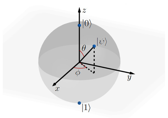
Figure 1.
Bloch sphere.
Now, a quantum algorithm is a set of gates acting on qubits in a specific order. This order is visualised in a quantum circuit, and an example can be found in Figure 2. The circuit should be designed such that the resulting quantum state is useful and provides the answer to a certain problem. Note that the outcome is probabilistic, and some algorithms will ask for a number of repetitions to translate the quantum state answer to an answer that can be used for further, conventional computing. Of course, the main goal of a quantum algorithm developer is to design an algorithm that outperforms the classical counterpart of the algorithm in terms of complexity. Famous examples of such algorithms are Shor’s and Grover’s. Shor’s algorithm [25] is a polynomial-time quantum computer algorithm for integer factorisation, which is expected to break certain types of cryptography. Grover’s algorithm [26] finds with high probability the unique input to a black box function with a domain of size N, only demanding function calls, whereas the classical algorithm requires function calls. The paper of [23] warns about some details of the proposed quantum algorithms. The data encoding phase and translating the quantum state outcome could even nullify the gained speed-up.

Figure 2.
Amplitude encoding: two-qubit circuit for data encoding of two normalised two-dimensional data points.
In most machine learning applications, data encoding is the first step in the algorithm. In Figure 2, a small example is shown of a quantum circuit, which we will use in the next sections of this paper, to encode two data points in two qubits.
A quantum circuit starts at the left side. Each line in the circuit represents a qubit, meaning we have two qubits in this example. Each cube represents a gate operation. In Figure 2, on the first qubit, we first apply a Hadamard gate. This gate brings the qubit into a superposition state as explained earlier. Then a controlled rotation is used to encode the two data points for in the amplitudes of the second qubit. Here, the angles of the rotations are chosen such that and . The initial state is now rotated to the desired state given by
Here, the first qubit acts as a counter, while the two features of the data point are encoded in the second qubit. Alternatively, using just two qubits, it is also possible to encode a single data point with four features.
To translate the circuit into the physical layout of the specific quantum computer, quantum programming languages can be used, such as QASM, PyQuil, QCL and Q#. These quantum programming languages only focus on a part of the quantum software stack [27], whilst tools for other layers are also in development.
2.2. Annealing-Based Quantum Computing
The second paradigm in quantum computing is quantum annealing. Quantum annealing started with the work of Kadowaki and Nishimori [28]. The main idea here is to create an equal superposition over all possible states. Then a problem-specific magnetic field is turned on, causing the qubits to interact with each other. Now, the qubits move towards the state with the lowest energy. The most advanced implementation of this paradigm is the D-Wave quantum annealer.
The main input of the D-Wave quantum annealer is an Ising Hamiltonian or its binary equivalent, the QUBO formulation. The quadratic unconstrained binary optimisation (QUBO) problem [29] is expressed by the optimisation problem:
where are the decision variables and Q is a coefficient matrix. QUBO problems belong to the class of NP-hard problems. For a large number of combinatorial optimisation problems, the QUBO representation is known [29,30]. Many constrained integer programming problems can easily be transformed into a QUBO representation.
To solve the problem that is formulated by the QUBO, it has to be embedded on the hardware. Each variable is translated into one or more (a chain of) qubits. The two most recent machines that are offered by D-Wave, via their LEAP environment, are the D-Wave 2000Q and the D-Wave Advantage. The D-Wave 2000Q has around 2000 qubits in a Chimera architecture, where each qubit is connected with at most six other qubits. The D-Wave Advantage, active since 2020, has more that 5000 qubits in the Pegasus architecture, having a connectivity of at most 15. However, while the number of qubits and their connectivity have grown considerably, they are still of limited size. This means that often the problem can not be embedded on the chip and has to be decomposed. D-Wave offers the possibility to control that process, but also offers built-in routines. The first decomposition algorithm introduced by D-Wave was qbsolv [31], which gave the possibility to solve larger-scale problems on the QPU. The new decomposition approaches D-Wave offers are D-Wave Hybrid and the Hybrid Solver Service, offering more flexibility.
3. Generating Data
The main case for this paper is indoor–outdoor detection. For the calculations, a dataset is generated. The proposed case is in the Universal Mobile Telecommunications System (UMTS) network. The data contain two features for the machine learning step: the received power level of the active connection and the received pilot signal to interference ratio. We use the simplified model from [32] and add extra loss to emulate the indoor environment, based on a simplified propagation model. The propagation model is:
or in logaritmic (dB) terms:
where
- : Received power level,
- : Transmitted power level,
- : Path loss/Attenuation,
- : Slow fading/Shadowing,
- : Fast fading/Multipath effects.
The level of the slow-faded power () fluctuates with a log-normal distribution around the received mean power. If the linear valued is log-normally distributed, then the logarithmic valued is normally distributed and expressed in dB, with parameters , where . Now, for a user at a certain location x receiving the signal from cell , neglecting the fast fading effect, we obtain (again in dB):
which is the first feature. Now we can define the second feature, the signal-to-interference ratio [33,34] of cell at the base station, having M interfering transmitters, as
Using this model, we generated 300 data points, using dBm, dB, and an additional path loss for indoor settings of 15 dB. As data preparation, we scaled the data to the interval and inverted the axis. The original data are shown in Figure 3, and the prepared data in Figure 4.
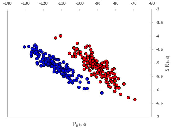
Figure 3.
Original generated data points. Red dots are the outdoor measurements, blue dots are the indoor measurements.
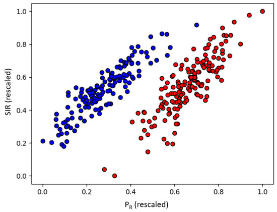
Figure 4.
Prepared artificial data points. Red dots are the outdoor measurements, blue dots are the indoor measurements.
4. Quantum Machine Learning Approaches
Three quantum machine learning algorithms, classifiers, are presented in this section. The first and the second algorithm are directed to the gate-based computer. The third approach is directed to the quantum annealer. For each of the approaches, we will explain whether real hardware or (conventional) emulators are used.
For each of the classifiers, we calculate the basic indicators Accuracy, Precision, Recall and -score on a validation data set as our key performance indicators. Accuracy (Acc) is the fraction of samples that have been classified correctly, Precision (Pr) is the proportion of correct positive identifications over all positive identifications, Recall (Rc) is the proportion of correct positive identifications over all actual positives:
where is the number of true positives, is the number of false positives, is the number of true negatives and is the number of false negatives. The -score is a way of combining the precision and recall of the model, and it is defined as the harmonic mean of the model’s precision and recall:
For the variational classifier and the SVM, we also look at the objective function that is being optimised in these cases.
4.1. Quantum Variational Classifier
The first approach we present is a variational classifier, where we used the implementation by pennylane.ai (https://pennylane.ai/qml/demos/tutorial_variational_classifier.html, accessed on 10 May 2021), inspired by [35]. The basic idea in these approaches is that a circuit is built using gates that perform rotations. Those rotations are comparable with the weight in a classical neural network and have to be learned. The goal then is to find those angles which result in output that best fits the expected output.
The input to the circuit is encoded using amplitude encoding in the qubits. The state preparation step for this was discussed earlier. On the values based on the state preparation, the model circuit is applied and a single qubit is measured to obtain the output. This is the general 3-step approach: 1. state preparation, 2. model circuit, 3. measurement. We now look in some more detail at the model circuit. This part works like a black box routine that executes the inference step of the machine learning algorithm on a small-scale quantum computer. Each layer consists of a generic single qubit gate rotating on all angles for each qubit and a controlled gate. Training of the angle parameters per qubit and layer is done by a classical gradient method. The data are already rescaled and are now also padded to have four features and then normalised (see Figure 5). Working on the positive subspace makes encoding of the data into the qubits much easier, as proposed in [36]. The used cost function is the standard square loss that measures the distance between the target labels and model predictions. An example of a 2-layer model circuit, including the data encoding, is shown in Figure 6, where Note that only one single data point with four features is encoded. This is different from the example in Section 2.1 where we gave an example of encoding two data points with two features. The required number of qubits in this model only depends on the number of features and not the size of the data set.
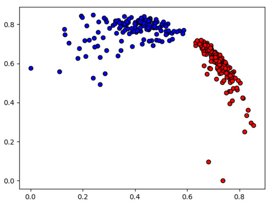
Figure 5.
Padded and normalised data. Red dots are the outdoor measurements, blue dots are the indoor measurements.

Figure 6.
A 2-layer model circuit.
Thus far, we have presented a model for a generic layer, however, more simplified versions of this model can in certain cases also result in a satisfactory classification. For example, by considering only rotations instead of a generic rotation. On the other hand, in the case where more qubits are available, the model can also be made more complex by duplicating the data encoding in multiple qubits, as shown in Figure 7 for a single-layer model.
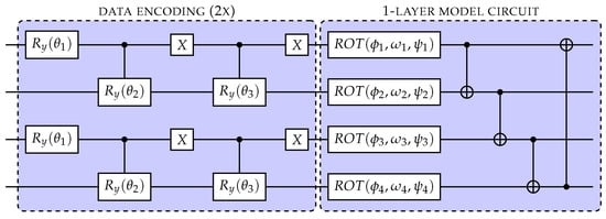
Figure 7.
A single-layer model circuit.
Encoding the data multiple times in the circuit can lead to faster training times and better predictions. The best choice of the variational circuit has conflicting considerations. On one hand, one tries to keep the circuit as simple as possible. This is especially important for implementations on real hardware where, due to noise, more errors occur when the circuit contains more gates. Furthermore, this lowers the number of parameters that need to be optimised and hence will result in faster training iterations. On the other hand, the model needs to be complex enough, such that it is able to express and classify the data to the degree that is desired. The best choice of the variational circuit depends, among other things, on the data and the available hardware and is still being actively researched.
For our data, we obtained the best results when using a 3-layer model on a quantum computer simulator. We implemented this using Python and a simple state simulator of qubit-based quantum circuit architectures [37], combined with a gradient-descent optimizer with Nesterov momentum [38], as offered by Pennylane. We compare a 2-qubit implementation to a 4-qubit implementation where we encode the same data point twice as described above. Nowadays, many quantum hardware providers, for example, IBM [39] or QuTech [40], offer free access to hardware back-ends with these numbers of qubits. The reason why we still opted to go with a simulating approach is because of the long training time when working using a real quantum device. The long training time is not caused by the circuit execution time, in fact, this often takes not much longer than milliseconds. It is, however, the queuing time, the time it takes for a circuit to be scheduled and run, which, when many users are active, can easily take multiple minutes and hence makes using a real device for our purposes infeasible. Furthermore, the choice of using a simulator allows us to make our layer models more complex.
We use of the data points as training data and the remaining as a validation set. In Figure 8, the cost objective function is shown as a function of the iterations which are being made by the classical gradient solver. It can be seen that the 4-qubit implementation, although having twice as many parameters that need to be optimised, requires fewer iterations before finding its loss plateau. Furthermore, the loss plateau for the 4-qubit solution appears to be lower than for the 2-qubit model. In Figure 9 and Figure 10, the decision regions after 350 iterations are shown for both models. We note that in both cases, all validation data points are assigned the correct label, and hence all performance indicators equal 1, see Table 1.
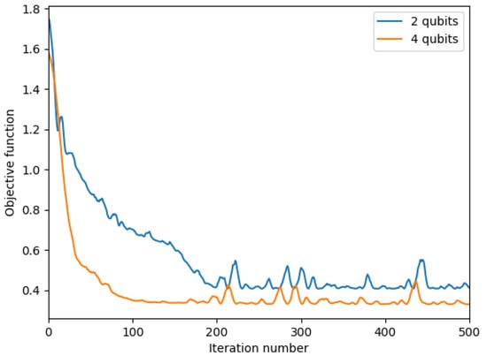
Figure 8.
Objective function variational classifier.
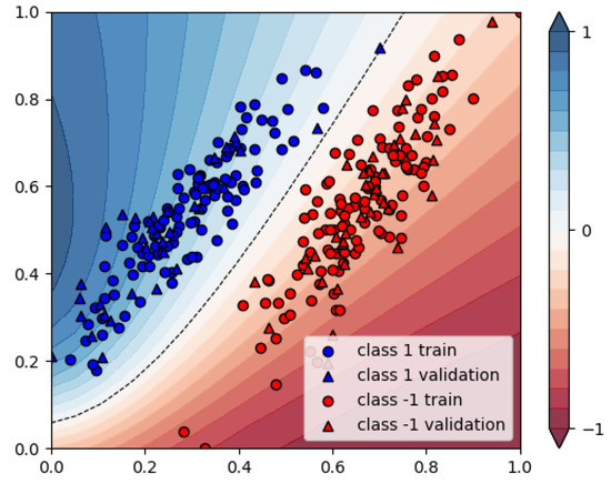
Figure 9.
Resulting assignments of the variational classifiers: 2-qubit model.
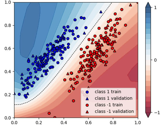
Figure 10.
Resulting assignments of the variational classifiers: 4-qubit model.

Table 1.
Overview of performance indicators after 350 optimisation iterations.
This approach has two main benefits according to [35]. Firstly, storing the parameters for later use is possible, while the hybrid classical–quantum approach stores these parameters classically, making them available outside the coherence time of the qubits. Secondly, this approach works well on a small quantum computer even for a large number of features and in the absence of strong error correction. An example in [35] shows that an eight-qubit model uses 100 parameters to classify inputs of dimensions, which is much more compact than a conventional feed-forward neural network.
4.2. Quantum Distance-Based Classifier
The second approach we present is a classification algorithm. Here, data points are classified based on their distance to the training data. The algorithm takes as input M training data points with binary labels . The goal of the algorithm is to assign a label to a new data point . Classification is based on the classification function
This method requires an additional preprocessing step to get the data in the required format. To be able to process the data by the qubits, they have to lie on a unit sphere. The implementation is explained in detail in [41]. The quantum algorithm can be implemented using qubits, where N is the number of training data points and F is the number of features of the data. In Figure 11, the resulting assignments are shown for and , which can be implemented on a quantum device using 20 qubits. In this figure, the projection on the unit sphere has been reverted before being plotted. Due to this projection on the unit sphere, it can be seen that classification of a data point depends only on the angle between the different features.
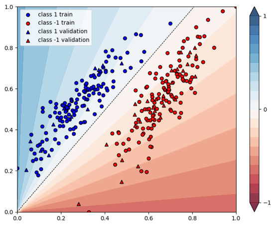
Figure 11.
Resulting assignments of the distance-based classifier with 256 training data points and 44 validation points.
This approach is especially powerful if the initial quantum state is given, for instance, as a result from a quantum process or using a quantum RAM, as was also proposed by [42]. In that case, the complexity is constant , independent of the number of features and the number of data points. If the quantum state has to be generated explicitly, the complexity is . Due to the probabilistic nature of quantum computing, the obtained result is probabilistic and multiple evaluations of the quantum state are required. The results are shown in Table 2.

Table 2.
Overview of performance indicators for the validation data set for the distance-based classification trained on 256 data points.
4.3. Quantum Annealing-Based SVM
The third approach is a quantum implementation of so-called kernel-based support vector machines (SVMs). SVMs are supervised machine learning algorithms for classification and regression problems. Willsch et al. proposed an approach to implement SVMs on a quantum annealer [43]. We use this approach and show the performance on the newest releases of the D-Wave quantum annealers. The approach involves the SVM being translated to a QUBO formulation. We assume a labelled dataset, containing N data points (), where is a feature vector and is the corresponding label. A first step is to formulate the SVM as a quadratic problem:
where is a coefficient, C a regularisation parameter and the kernel function. A commonly used kernel is the Gaussian kernel , using a hyperparameter . The coefficients define a decision boundary that separates the vector space into two regions, corresponding to the predicted class labels. To translate this quadratic programming formulation to a QUBO formulation, there are two main steps. First, the -values have to be translated to binary input, using the encoding:
with binary variables, K being the number of binary variables to encode and B being the base used for the encoding, usually or . More details about the choice for K can be found in [43]. The second step is to translate the constraints to the objective function, using a penalty factor for a quadratic penalty. The resulting objective function then becomes:
If we want to solve this QUBO using the D-Wave hardware, the first approach is to directly embed this problem on the quantum chip. However, D-Wave also offers ready-to-use alternatives to solve the QUBO conventionally using simulated annealing. In this way, the problem does not have to be decomposed and can be calculated directly as a benchmark of using the QPU. In this implementation we also use cases where the ratio between the training data and the validation set equals . We use the parameters , , , and . Starting with the simulated annealing solver, we get the results as shown in Figure 12.
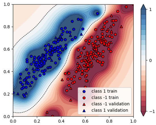
Figure 12.
Resulting assignments of the simulated annealing-based SVM, 225 datapoints.
Using the QPU, we are restricted by the size of the current architecture, namely 2000 qubits in a Chimera architecture or the 5000 qubits in the latest Pegasus architecture. Pegasus qubits have a degree of 15, i.e., they are externally coupled to 15 different qubits. When the problem is embedded onto the qubit structure, the number of available qubits and the limitations lead to problems. In most cases, it is not possible to find a correct embedding. Problem decomposition techniques can help to cut the problem into pieces, where each piece is solved separately and then combined back together. However, this is at the expense of the quality of the solution.
First, we investigate what the biggest problem is that can be embedded on each of the available machines, without using decomposition techniques. For the Chimera architecture, this means using 25 data points for learning and 8 for validation. For the Pegasus architecture, this means 70 data points for learning and 23 for validation. The QPU uses less than 10 ms of annealing time for solving this problem. The results for these problems can be found in Figure 13 and Figure 14. For reference, the result from the simulated annealing approach for the same data and the same parameters is also presented in Figure 15 and Figure 16.
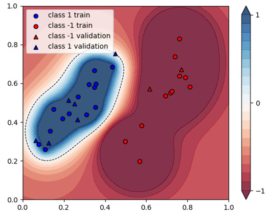
Figure 13.
Resulting assignments of the quantum annealing-based SVM, 25 datapoints.
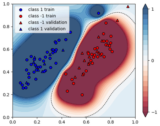
Figure 14.
Resulting assignments of the quantum annealing-based SVM, 70 datapoints.
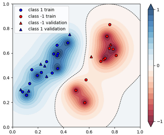
Figure 15.
Resulting assignments of the simulated annealing-based SVM, 25 datapoints.
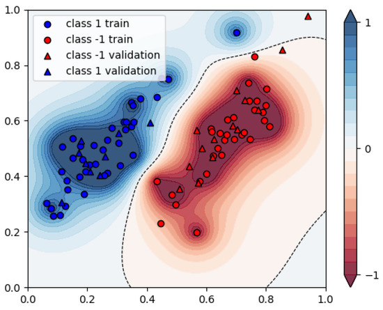
Figure 16.
Resulting assignments of the simulated annealing-based SVM, 70 datapoints.
If we do want to use decomposition techniques, the D-Wave system employs built-in routines to decompose the problem into smaller sub-problems that are sent to the QPU, and in the end reconstructs the complete solution vector from all sub-sample solutions. Here, we use D-Wave’s Hybrid Solver, which implements state-of-the-art classical algorithms with intelligent allocation of the QPU to parts of the problem where it benefits most, i.e., the sampler uses the energy impact as the criterion for the selection of variables. These solvers are designed to accommodate even very large problems. This means that most parameters of the embedding are set automatically. By default, samples are iterated over four parallel solvers. The top branch implements a classical Tabu Search that runs on the entire problem until interrupted by another branch completing. The other three branches use different decomposers to sample out parts of the current sample set and send it to different samplers. HQPU acts as a black box solver and the specific part of the problem which gets embedded on the QPU is unknown. The hybrid solver can solve the problem using 225 data points and 75 validation points, and is faster than simulated annealing, with approximately the same result (see Figure 17).
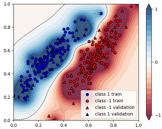
Figure 17.
Resulting assignments of the Hybrid Solver-based SVM, 225 data points.
We show the results using the performance indicators Accuracy, -score, Precision and Recall as our KPIs again. Lastly, we present the energy of every solution, which is the score generated by the objective function in Equation (15). To give some idea about the optimal values, we also use the commercially available solver LocalSolver (www.localsolver.com, accessed on 10 May 2021), to solve both the original problem expressed by Equations (11)–(14) and the QUBO problem expressed by Equation (15). For all problems, a solution is found quickly, however, after 60 s, optimality gaps of 40–99% still remain. To make the comparison somewhat fair, we also give the Hybrid Solver one minute of calculation time, Simulated Annealing 4000 reads (resulting in one minute of calculation time) and the QPU 4000 reads as well (around 80 ms of calculation time). The scores for the three cases, using 25, 70 and 225 data points for training, are depicted in Table 3. We see that for almost all cases, the performance is good, all validation data points are labelled correctly. Only in the case is there one point that is not labelled correctly in the case of the simulated annealing and the direct use of the QPU. The Hybrid Solver does label this point correctly. The main difference is found in the energy level, meaning the objective value. The best solution for all cases is found by LocalSolver, solving the original problem. The Hybrid Solver is the best performing approach of all quantum (inspired) approaches in all cases. The direct implementation on the QPU performs worst, which can be seen in the heat maps, where the direct QPU solution has a large area where the score is equal to one. LocalSolver also has problems solving the QUBO problem, probably due to the lack of structure of the problem.

Table 3.
Overview of results.
5. Conclusions
Communication networks are managed more and more by using artificial intelligence. Anomaly detection, network monitoring and user behaviour are areas where machine learning offer advantages over more traditional methods. However, increasingly, computing power is a limited factor in machine learning tasks. For mobile network operators, it is becoming more and more important to be able to classify the location of mobile devices, to enhance network performance and to offer location-based services. The rise of quantum computers might bring the next step needed here. In particular, machine learning is seen as a promising task for the first generation of quantum computers. In this paper, we proposed three machine learning approaches for indoor–outdoor classification. These techniques are expected to be useful on the near-term hardware.
The first approach is a quantum variational classifier. This approach only uses a small number of qubits and is able to manage a larger number of data points. The expected gain here is not the calculation time. The compactness of the formulation will be of added value, which will lead to more efficient learning of a model with multiple features. Next, we compared a 2-qubit implementation to a 4-qubit implementation. We showed that the 4-qubit implementation, although having twice as many parameters that needed to be optimised, required fewer iterations before finding its loss plateau.
The quantum distance-based classifier brings the complexity back to , independent of the number of features and the number of data points. However, the data management is a big problem at this moment. The number of qubits needed to store big data input and the time it takes to encode the data are still under scientific investigation.
The quantum annealing-based SVM is the most straightforward implementation of a conventional approach. Using the Hybrid Solver gave us the possibility to solve bigger problems than in the case where a direct implementation on the chip was realised. The expectation here is that the solution will scale better than conventional approaches when the underlying hardware grows.
For further research, we are interested in how well the methods perform on more messy, imbalanced datasets and in some indications of the performance on full-size data sets. Lastly, we are interested in the level of convergence of the quantum variational classifier for more generic data sets.
Author Contributions
Conceptualization, F.P., R.S.W. and I.C.; methodology, F.P.; software, R.S.W. and I.C.; validation, F.P.; writing—original draft preparation, F.P. and R.S.W.; writing—review and editing, I.C.; visualization, R.S.W.; supervision, F.P.; project administration, F.P.; funding acquisition, F.P.; All authors have read and agreed to the published version of the manuscript.
Funding
This research received no external funding.
Institutional Review Board Statement
Not applicable.
Informed Consent Statement
Not applicable.
Data Availability Statement
Authors can confirm that all relevant data are included in the article.
Conflicts of Interest
The authors declare no conflict of interest.
References
- Wang, W.; Chang, Q.; Li, Q.; Shi, Z.; Chen, W. Indoor-outdoor detection using a smart phone sensor. Sensors 2016, 16, 1563. [Google Scholar] [CrossRef] [PubMed]
- Esmaeili Kelishomi, A.; Garmabaki, A.; Bahaghighat, M.; Dong, J. Mobile user indoor-outdoor detection through physical daily activities. Sensors 2019, 19, 511. [Google Scholar] [CrossRef]
- Saffar, I.; Morel, M.L.A.; Singh, K.D.; Viho, C. Machine Learning with partially labeled Data for Indoor Outdoor Detection. In Proceedings of the 2019 16th IEEE Annual Consumer Communications & Networking Conference (CCNC), Las Vegas, NV, USA, 11–14 January 2019; pp. 1–8. [Google Scholar]
- Saffar, I.; Morel, M.L.A.; Amara, M.; Singh, K.D.; Viho, C. Mobile User Environment Detection using Deep Learning based Multi-Output Classification. In Proceedings of the 2019 12th IFIP Wireless and Mobile Networking Conference (WMNC), Paris, France, 11–13 September 2019; pp. 16–23. [Google Scholar]
- Zhang, L.; Ni, Q.; Zhai, M.; Moreno, J.; Briso, C. An ensemble learning scheme for indoor-Outdoor classification based on KPIs of LTE network. IEEE Access 2019, 7, 63057–63065. [Google Scholar] [CrossRef]
- Bejarano-Luque, J.L.; Toril, M.; Fernandez-Navarro, M.; Acedo-Hernández, R.; Luna-Ramírez, S. A Data-Driven Algorithm for Indoor/Outdoor Detection Based on Connection Traces in a LTE Network. IEEE Access 2019, 7, 65877–65888. [Google Scholar] [CrossRef]
- Zhu, Y.; Luo, H.; Wang, Q.; Zhao, F.; Ning, B.; Ke, Q.; Zhang, C. A fast indoor/outdoor transition detection algorithm based on machine learning. Sensors 2019, 19, 786. [Google Scholar] [CrossRef]
- Leiserson, C.E.; Thompson, N.C.; Emer, J.S.; Kuszmaul, B.C.; Lampson, B.W.; Sanchez, D.; Schardl, T.B. There’s plenty of room at the Top: What will drive computer performance after Moore’s law? Science 2020, 368, eaam9744. [Google Scholar] [CrossRef]
- Dunjko, V.; Taylor, J.M.; Briegel, H.J. Quantum-enhanced machine learning. Phys. Rev. Lett. 2016, 117, 130501. [Google Scholar] [CrossRef] [PubMed]
- Neumann, N.M.P.; Phillipson, F.; Versluis, R. Machine learning in the quantum era. Digit. Welt 2019, 3, 24–29. [Google Scholar] [CrossRef]
- Phillipson, F. Quantum Machine Learning: Benefits and Practical Examples. In Proceedings of the International Workshop on QuANtum SoftWare Engineering & pRogramming (QANSWER), Talavera de la Reina, Spain, 11–12 February 2020; pp. 51–56. [Google Scholar]
- Schuld, M.; Sinayskiy, I.; Petruccione, F. An introduction to quantum machine learning. Contemp. Phys. 2015, 56, 172–185. [Google Scholar] [CrossRef]
- Abohashima, Z.; Elhosen, M.; Houssein, E.H.; Mohamed, W.M. Classification with Quantum Machine Learning: A Survey. arXiv 2020, arXiv:2006.12270. [Google Scholar]
- Biamonte, J.; Wittek, P.; Pancotti, N.; Rebentrost, P.; Wiebe, N.; Lloyd, S. Quantum machine learning. Nature 2017, 549, 195–202. [Google Scholar] [CrossRef] [PubMed]
- Low, G.H.; Yoder, T.J.; Chuang, I.L. Quantum inference on Bayesian networks. Phys. Rev. A 2014, 89, 062315. [Google Scholar] [CrossRef]
- Kapoor, A.; Wiebe, N.; Svore, K. Quantum perceptron models. In Proceedings of the 30th International Conference on Neural Information Processing Systems, Barcelona, Spain, 5–10 December 2016; pp. 3999–4007. [Google Scholar]
- Neumann, N.M.P.; de Heer, P.B.U.L.; Chiscop, I.; Phillipson, F. Multi-agent reinforcement learning using simulated quantum annealing. In Proceedings of the International Conference on Computational Science, Amsterdam, The Netherlands, 3–5 June 2020; Springer: Cham, Switzerland, 2020; pp. 562–575. [Google Scholar]
- Lloyd, S.; Mohseni, M.; Rebentrost, P. Quantum principal component analysis. Nat. Phys. 2014, 10, 631–633. [Google Scholar] [CrossRef]
- Rebentrost, P.; Mohseni, M.; Lloyd, S. Quantum support vector machine for big data classification. Phys. Rev. Lett. 2014, 113, 130503. [Google Scholar] [CrossRef] [PubMed]
- Wiebe, N.; Braun, D.; Lloyd, S. Quantum algorithm for data fitting. Phys. Rev. Lett. 2012, 109, 050505. [Google Scholar] [CrossRef] [PubMed]
- Dunjko, V.; Briegel, H.J. Machine learning & artificial intelligence in the quantum domain: A review of recent progress. Rep. Prog. Phys. 2018, 81, 074001. [Google Scholar]
- Harrow, A.W.; Hassidim, A.; Lloyd, S. Quantum algorithm for linear systems of equations. Phys. Rev. Lett. 2009, 103, 150502. [Google Scholar] [CrossRef]
- Aaronson, S. Read the fine print. Nat. Phys. 2015, 11, 291–293. [Google Scholar] [CrossRef]
- Resch, S.; Karpuzcu, U.R. Quantum computing: An overview across the system stack. arXiv 2019, arXiv:1905.07240. [Google Scholar]
- Shor, P.W. Polynomial-time algorithms for prime factorization and discrete logarithms on a quantum computer. SIAM Rev. 1999, 41, 303–332. [Google Scholar] [CrossRef]
- Grover, L.K. A Fast Quantum Mechanical Algorithm for Database Search. In Proceedings of the Twenty-Eighth Annual ACM Symposium on Theory of Computing (STOC ’96), Philadephia, PA, USA, 22–24 May 1996; Association for Computing Machinery: New York, NY, USA, 1996; pp. 212–219. [Google Scholar] [CrossRef]
- van den Brink, R.F.; Phillipson, F.; Neumann, N.M.P. Vision on Next Level Quantum Software Tooling. In Proceedings of the Tenth International Conference on Computational Logics, Algebras, Programming, Tools, and Benchmarking, Venice, Italy, 5–9 May 2019. [Google Scholar]
- Kadowaki, T.; Nishimori, H. Quantum annealing in the transverse Ising model. Phys. Rev. E 1998, 58, 5355. [Google Scholar] [CrossRef]
- Glover, F.; Kochenberger, G.; Du, Y. A tutorial on formulating and using qubo models. arXiv 2018, arXiv:1811.11538. [Google Scholar]
- Lucas, A. Ising formulations of many NP problems. Front. Phys. 2014, 2, 5. [Google Scholar] [CrossRef]
- Booth, M.; Reinhardt, S.P.; Roy, A. Partitioning Optimization Problems for Hybrid Classical/Quantum Execution; Technical Report; D-Wave Systems: Burnaby, BC, Canada, 2017. [Google Scholar]
- Erdbrink, R. Analysis of UMTS Cell Assignment Probabilities. Master’s Thesis, VU University Amsterdam, Amsterdam, The Netherlands, 2005. [Google Scholar]
- Haenggi, M.; Andrews, J.G.; Baccelli, F.; Dousse, O.; Franceschetti, M. Stochastic geometry and random graphs for the analysis and design of wireless networks. IEEE J. Sel. Areas Commun. 2009, 27, 1029–1046. [Google Scholar] [CrossRef]
- Tsalaile, T.; Sameni, R.; Sanei, S.; Jutten, C.; Chambers, J. Sequential blind source extraction for quasi-periodic signals with time-varying period. IEEE Trans. Biomed. Eng. 2008, 56, 646–655. [Google Scholar] [CrossRef]
- Schuld, M.; Bocharov, A.; Svore, K.M.; Wiebe, N. Circuit-centric quantum classifiers. Phys. Rev. A 2020, 101, 032308. [Google Scholar] [CrossRef]
- Schuld, M. Supervised Learning with Quantum Computers; Springer: Cham, Switzerland, 2018. [Google Scholar]
- PennyLane Simulator. Available online: https://pennylane.readthedocs.io/en/stable/code/api/pennylane.device.html#pennylane.device (accessed on 10 May 2021).
- Gradient-Descent Optimizer with Nesterov Momentum. Available online: https://pennylane.readthedocs.io/en/stable/code/api/pennylane.NesterovMomentumOptimizer.htmlm (accessed on 10 May 2021).
- IBM Quantum Computing. Available online: www.ibm.com/quantum-computing/ (accessed on 10 May 2021).
- QuTech Quantum Inpire. Available online: www.quantum-inspire.com (accessed on 10 May 2021).
- Wezeman, R.; Neumann, N.; Phillipson, F. Distance-based classifier on the Quantum Inspire. Digit. Welt 2020, 4, 85–91. [Google Scholar] [CrossRef]
- Schuld, M.; Fingerhuth, M.; Petruccione, F. Implementing a distance-based classifier with a quantum interference circuit. EPL (Europhys. Lett.) 2017, 119, 60002. [Google Scholar] [CrossRef]
- Willsch, D.; Willsch, M.; De Raedt, H.; Michielsen, K. Support vector machines on the D-Wave quantum annealer. Comput. Phys. Commun. 2020, 248, 107006. [Google Scholar] [CrossRef]
Publisher’s Note: MDPI stays neutral with regard to jurisdictional claims in published maps and institutional affiliations. |
© 2021 by the authors. Licensee MDPI, Basel, Switzerland. This article is an open access article distributed under the terms and conditions of the Creative Commons Attribution (CC BY) license (https://creativecommons.org/licenses/by/4.0/).