
Network Analysis of Local Gene Regulators in Arabidopsis thaliana under Spaceflight Stress

 ,
,  , ,
, ,
Abstract
1. Introduction
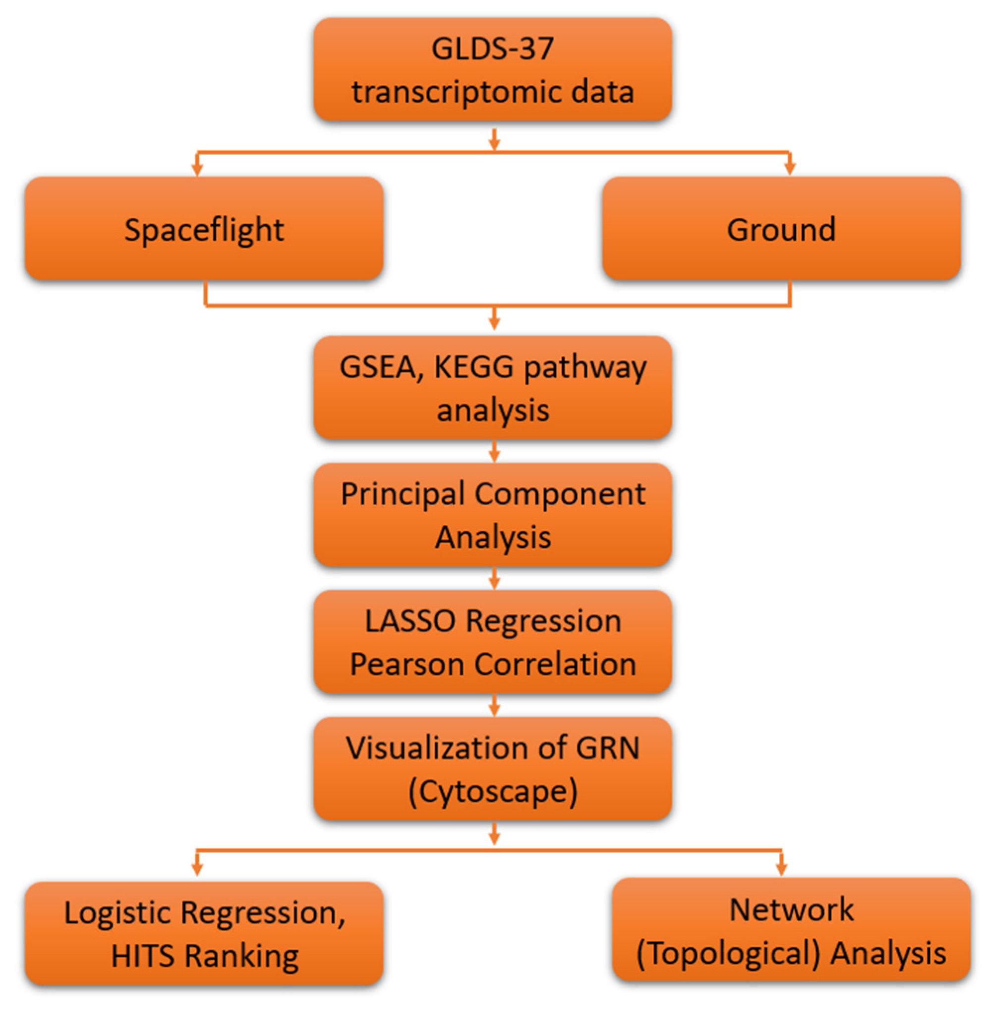
2. Materials and Methods
2.1. GeneLab Arabidopsis thaliana Dataset
2.2. GSEA and KEGG Pathway Analysis
2.3. Principal Component Analysis
2.4. Lasso Regression
2.5. Logistic Regression Based Gene Ranking
2.6. Network Analysis
2.6.1. Fold-Change
2.6.2. Graphs and Networks
| Algorithm 1 pseudocode | |
| HITS(A): # A :=(The adjacency matrix of the weighted network N = (V,E)) | |
| ; | # |
| ; | #’ |
| m; | # the number of HITS iterations. |
| # all entries in h are 1 | |
| # all entries in the vector are 1. | |
| ; | |
| ; | |
| whiledo; | |
| begin; | |
| ; | |
| # norm(v) = square-root of sum of squares | |
| ; | |
| end | |
- Vertex step: Add a new vertex and an edge from to by randomly and independently choosing proportional its degree;
- Edge step: Add a new edge by independently choosing vertices and with probability proportional to their degrees.
3. Results
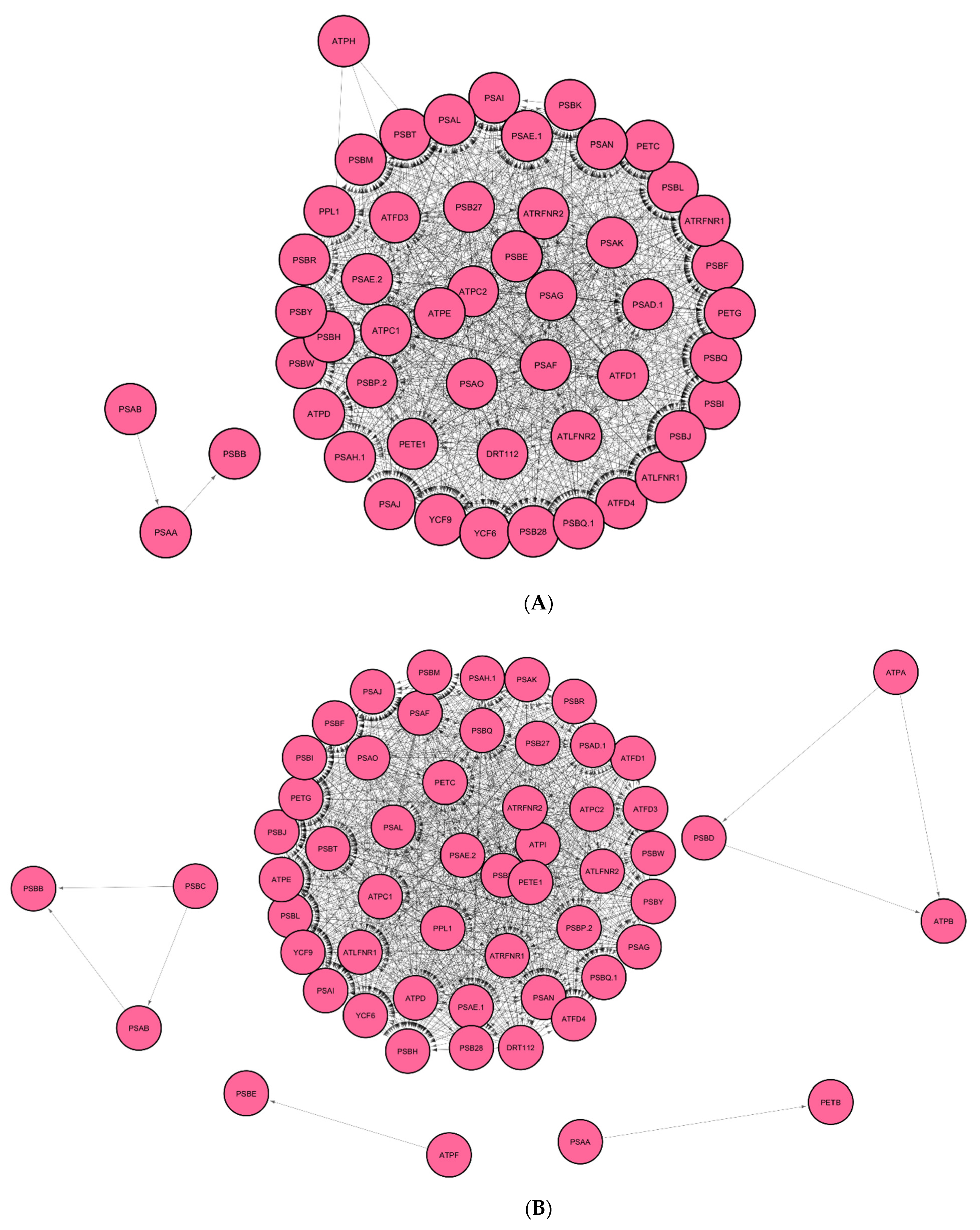
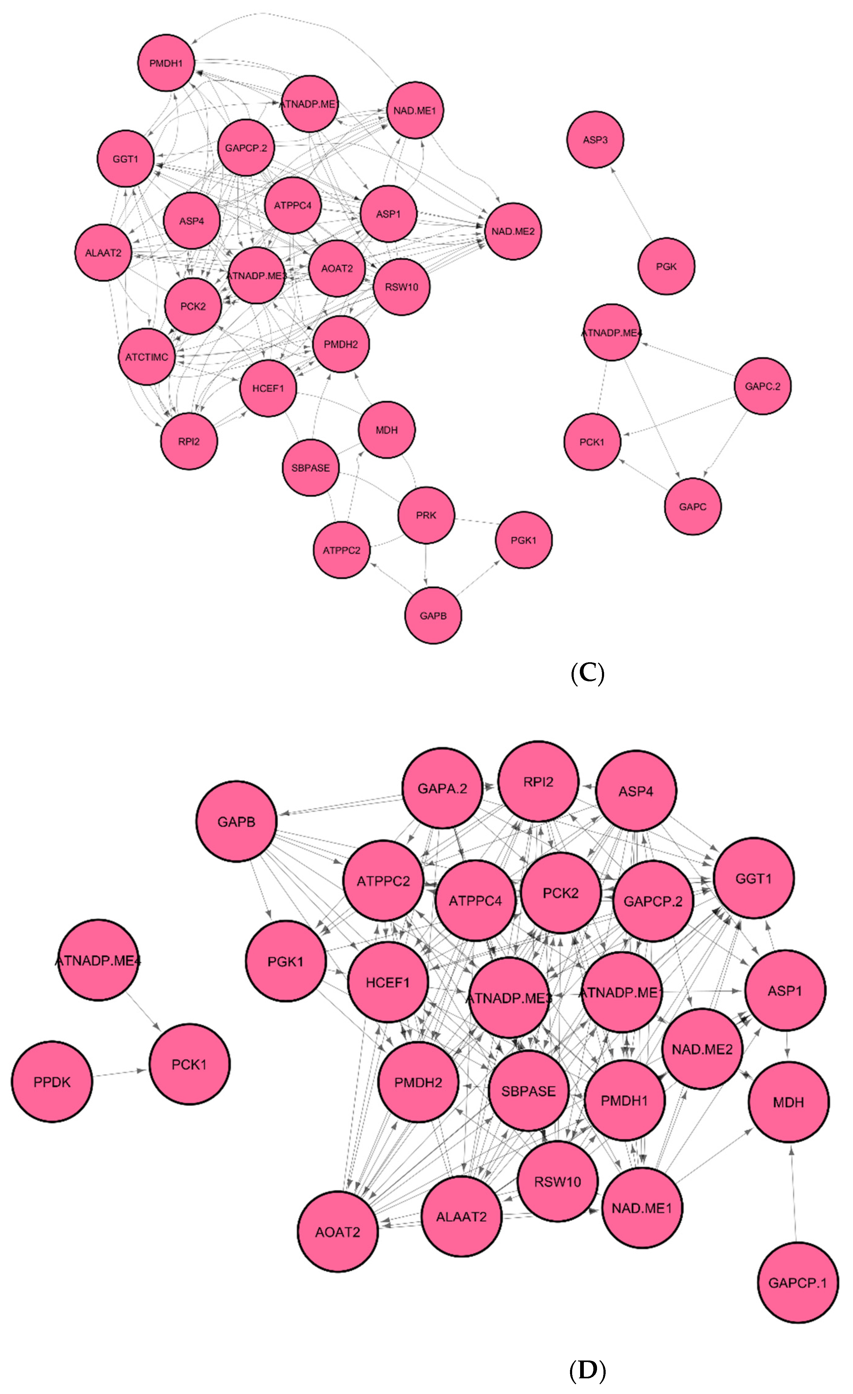
3.1. Identification of Regulatory Hub-Genes in Photosynthesis and Carbon Fixation GRN
3.2. Identification of Stress Response Genes in GRN of Spaceflight Microgravity and Ground Control
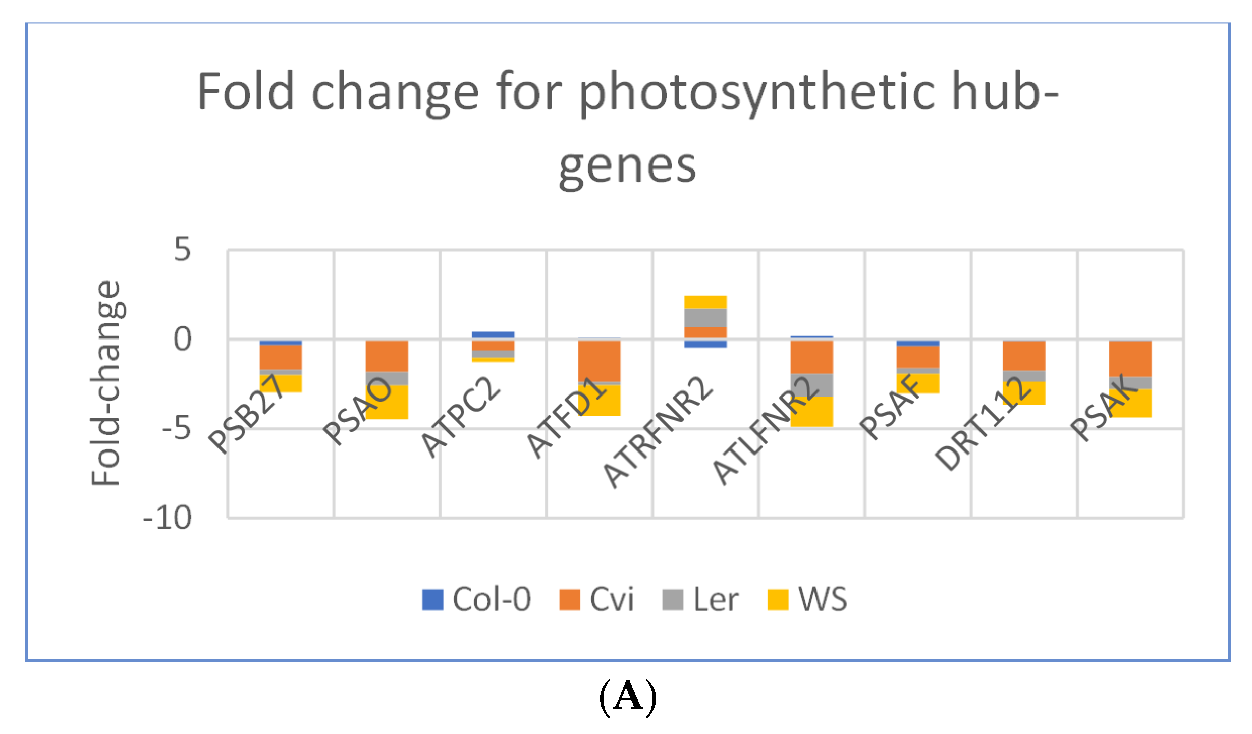
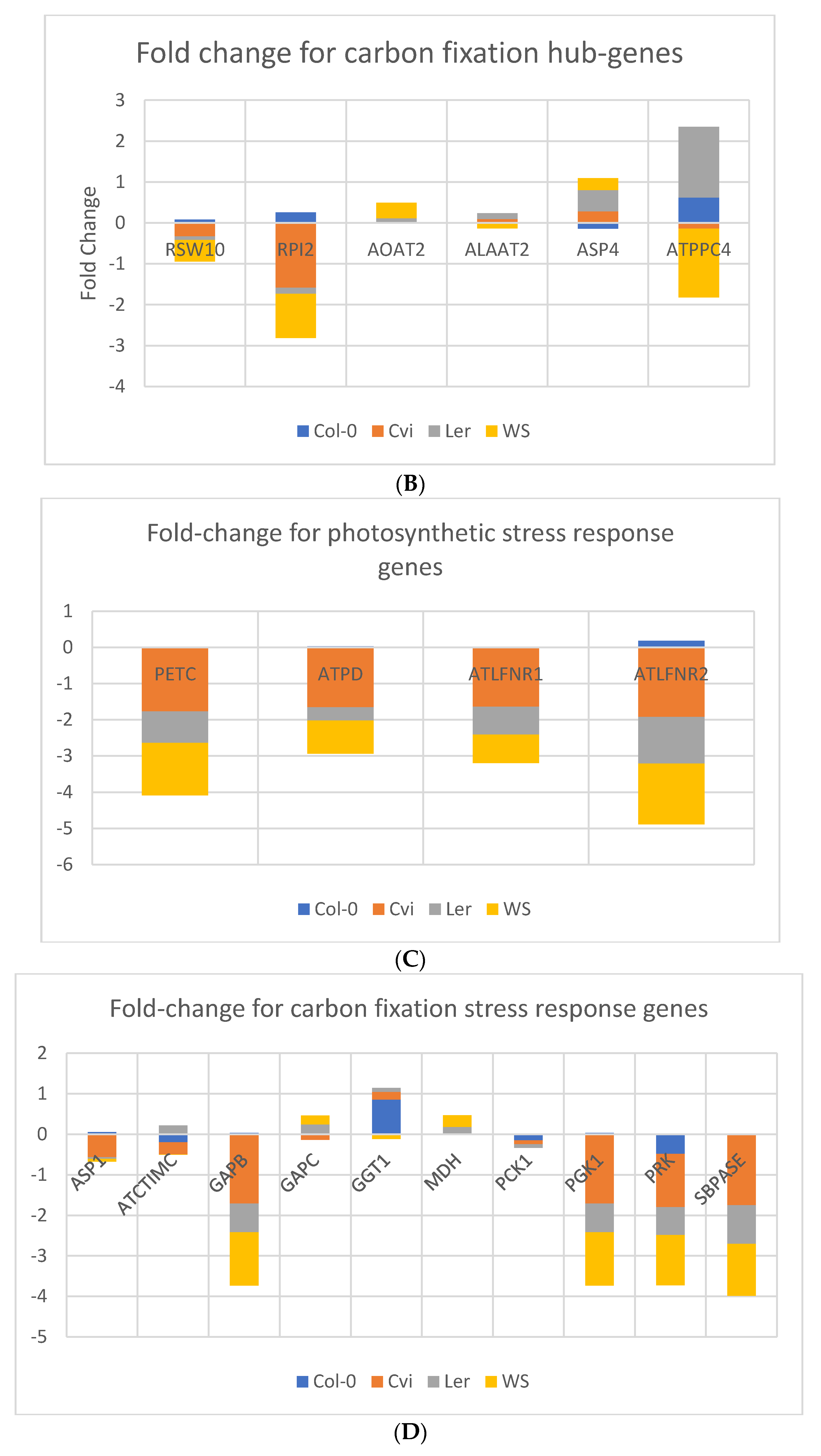
3.3. Photosynthesis Genes are Downregulated in Spaceflight Microgravity
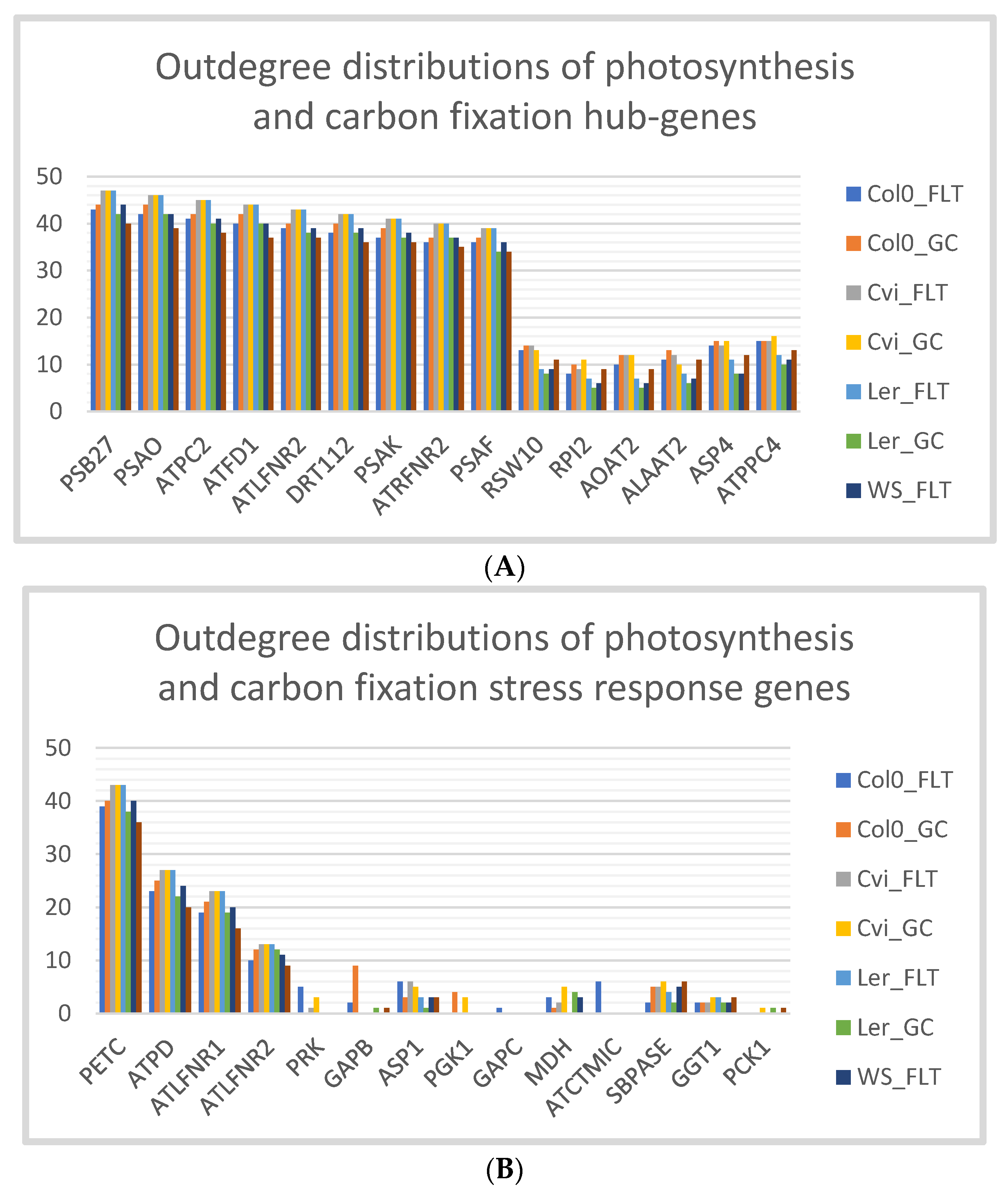
3.4. Cvi Ecotype has the Same Outdegree Distributions in Spaceflight Microgravity and Ground Control
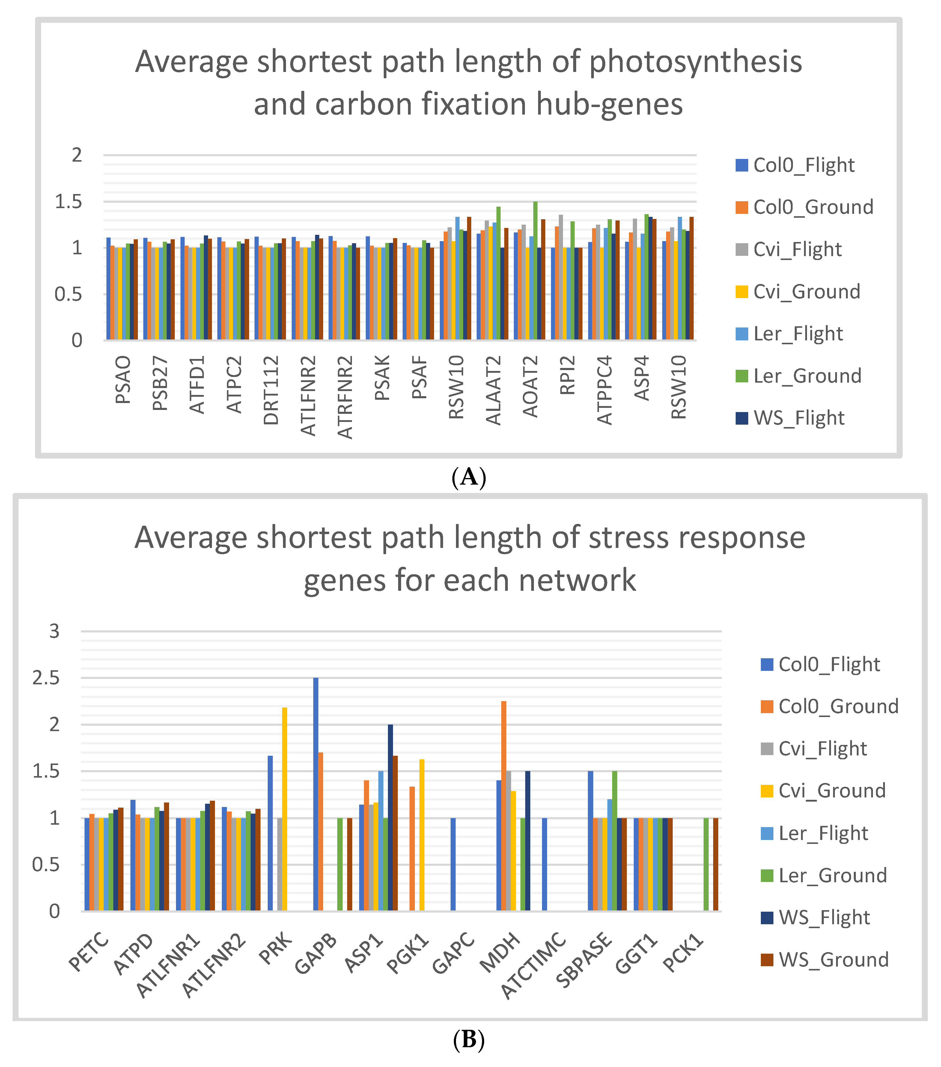
3.5. Stress Response Genes of Col-0 Ecotype have Low Shortest Path Lengths in Spaceflight Microgravity
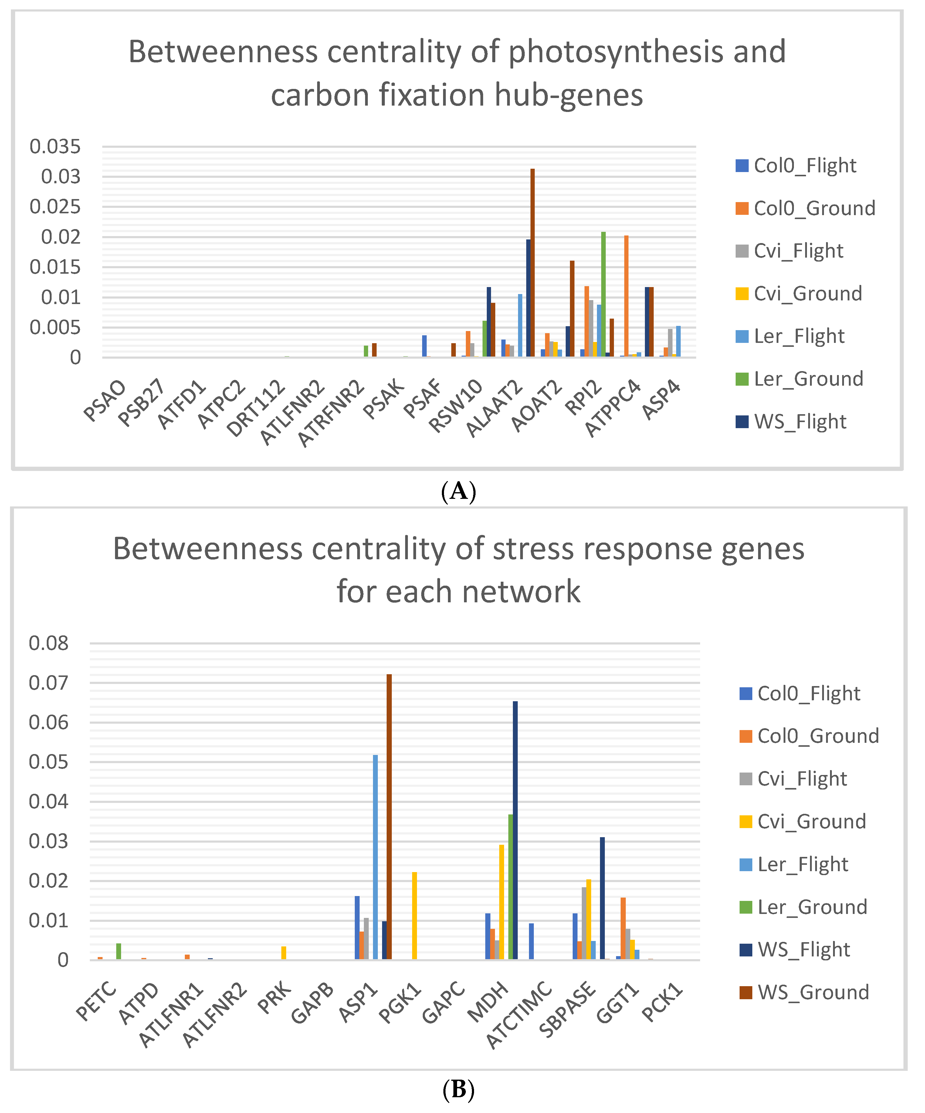
3.6. Photosynthesis Hub-Genes Have Low Betweenness Centrality
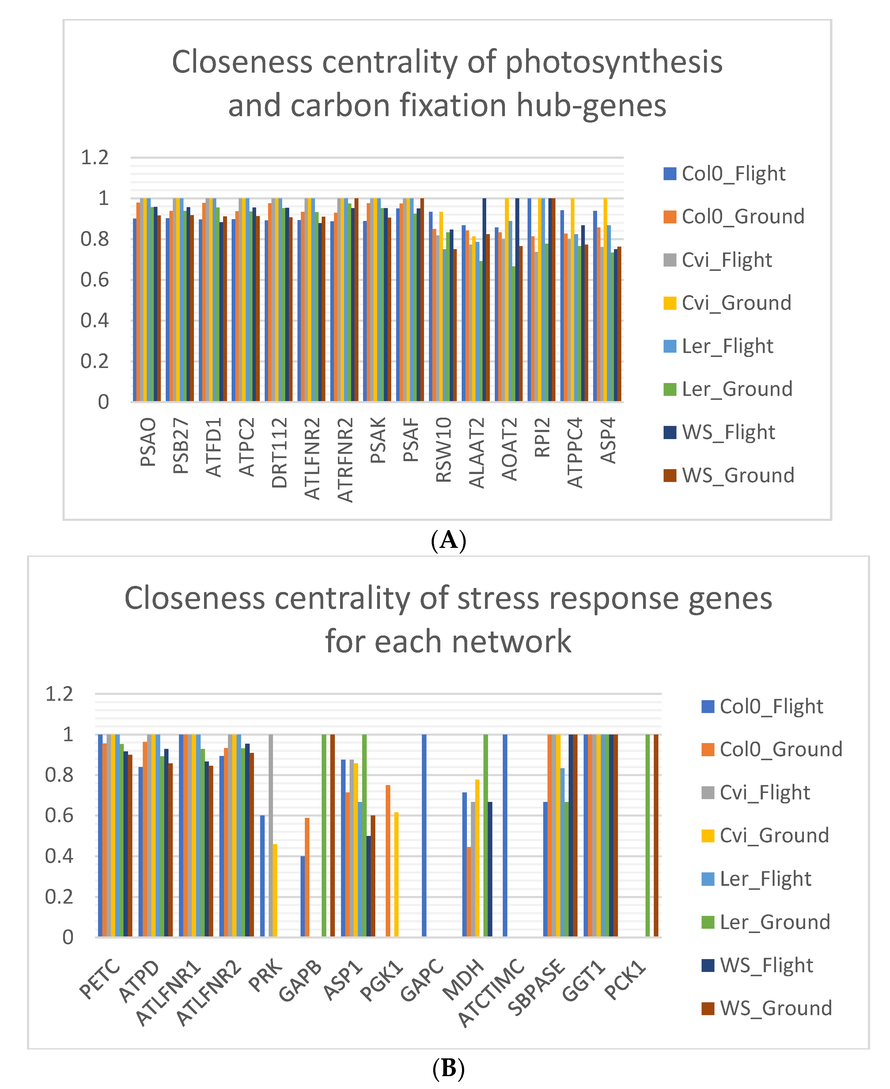
3.7. Closeness Centrality is Lowered in Spaceflight Microgravity
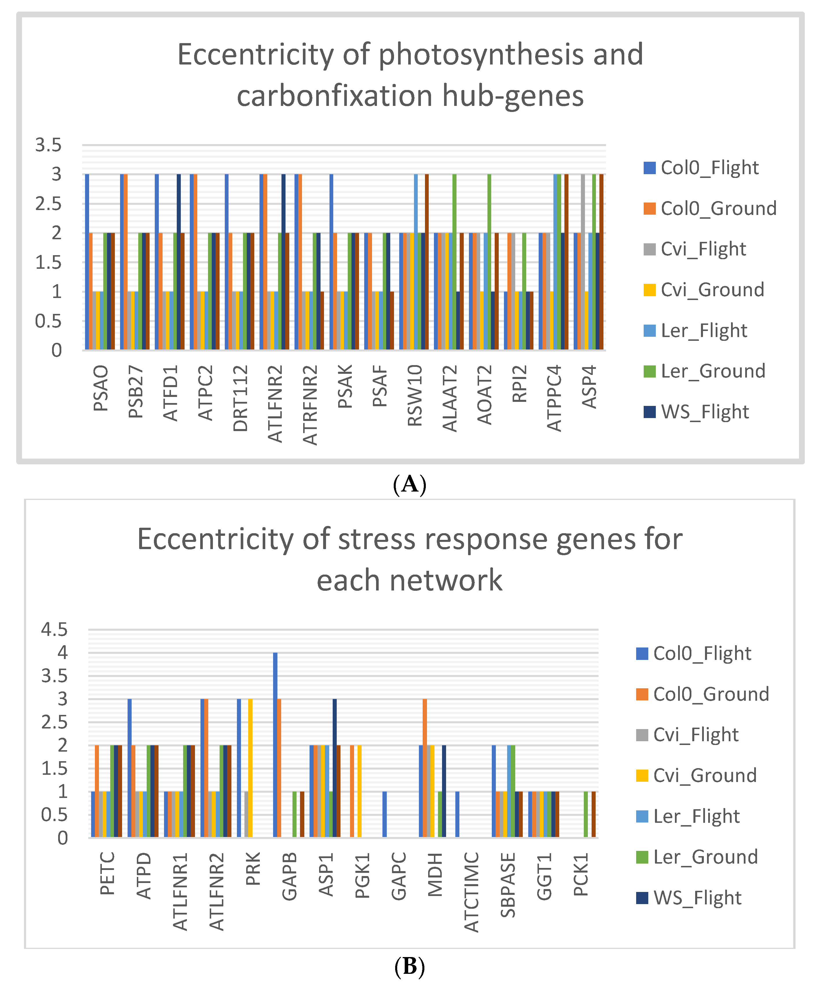
3.8. Col-0 Ecotype Hub-Genes Have High Eccentricity in Spaceflight Microgravity Compared to Ground Control
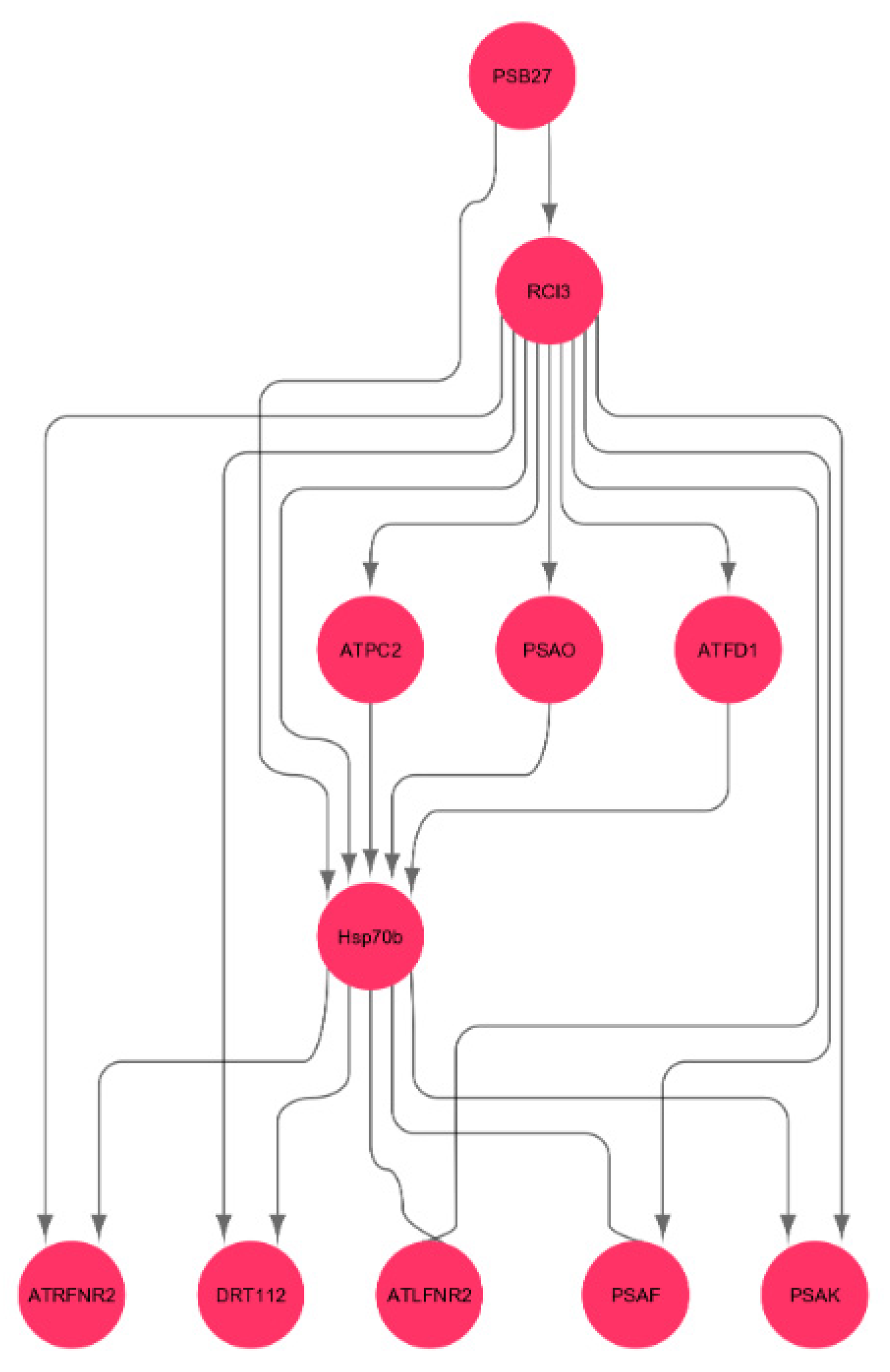
3.9. Interactions of Oxidative Stress Response Genes with Photosynthesis Hub-Genes
4. Discussion
4.1. Low Shortest Path Length Indicates Small-World-Ness of the Network
4.2. High Network Centrality Indicates the Importance of Genes on the Whole Network
4.3. High Eccentricity Indicates Higher Connections in the Network
4.4. Heat Shock Gene Regulates Photosynthesis Genes in Spaceflight Microgravity
4.5. Spaceflight Environment Leads to Dehydration-and-Salt-Stress Sensitive Ecotypes
4.6. Results from the Network Analysis
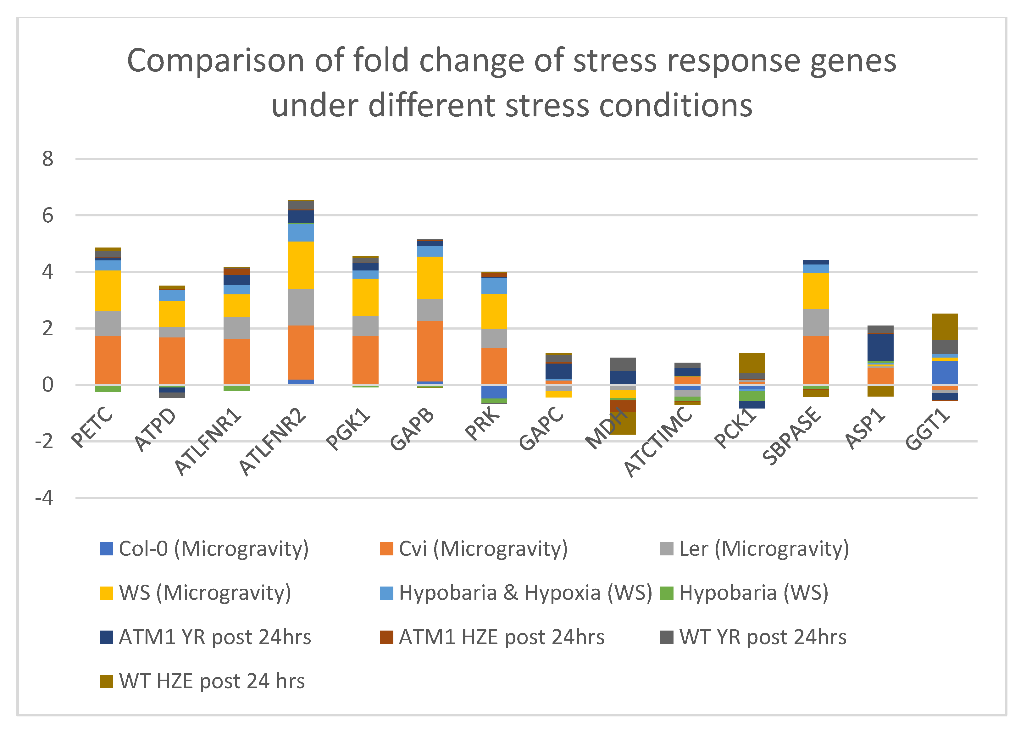
4.7. Comparison of the Stress Response Genes in Photosynthesis and Carbon fixation Processes of Arabidopsis thaliana under Different Stress Conditions
5. Conclusions
Supplementary Materials
Author Contributions
Funding
Institutional Review Board Statement
Informed Consent Statement
Data Availability Statement
Acknowledgments
Conflicts of Interest
References
- Koornneef, M.; Meinke, D. The development of Arabidopsis as a model plant. Plant J. 2010, 61, 909–921. [Google Scholar] [CrossRef] [PubMed]
- Initiative, T.A.G. Analysis of the genome sequence of Arabidopsis thaliana. Nature 2000, 408, 796–815. [Google Scholar] [CrossRef] [PubMed]
- Oakley, C.G.; Savage, L.; Lotz, S.; Larson, G.R.; Thomashow, M.F.; Kramer, D.M.; Schemske, D.W. Genetic basis of photosynthetic responses to cold in two locally adapted populations of Arabidopsis thaliana. J. Exp. Bot. 2018, 69, 699–709. [Google Scholar] [CrossRef] [PubMed]
- Paul, A.-L.; Sng, N.J.; Zupanska, A.K.; Krishnamurthy, A.; Schultz, E.R.; Ferl, R.J. Genetic dissection of the Arabidopsis spaceflight transcriptome: Are some responses dispensable for the physiological adaptation of plants to spaceflight? PLoS ONE 2017, 12, e0180186. [Google Scholar] [CrossRef] [PubMed]
- Bouchabke, O.; Chang, F.; Simon, M.; Voisin, R.; Pelletier, G.; Durand-Tardif, M. Natural Variation in Arabidopsis thaliana as a Tool for Highlighting Differential Drought Responses. PLoS ONE 2008, 3, e1705. [Google Scholar] [CrossRef] [PubMed]
- Barah, P.; Jayavelu, N.D.; Mundy, J.; Bones, A.M. Genome scale transcriptional response diversity among ten ecotypes of Arabidopsis thaliana during heat stress. Front. Plant Sci. 2013, 4. [Google Scholar] [CrossRef][Green Version]
- Wang, Y.; Yang, L.; Zheng, Z.; Grumet, R.; Loescher, W.; Zhu, J.-K.; Yang, P.; Hu, Y.; Chan, Z. Transcriptomic and Physiological Variations of Three Arabidopsis Ecotypes in Response to Salt Stress. PLoS ONE 2013, 8, e69036. [Google Scholar] [CrossRef]
- Prasch, C.M.; Sonnewald, U. In silico selection of Arabidopsis thaliana ecotypes with enhanced stress tolerance. Plant Signal. Behav. 2013, 8, e26364. [Google Scholar] [CrossRef]
- Li, P.; Mane, S.P.; Sioson, A.A.; Vasquez-Robinet, C.; Heath, L.S.; Bohnert, H.J.; Grene, R. Effects of chronic ozone exposure on gene expression in Arabidopsis thaliana ecotypes and in Thellungiella halophila. Plant Cell Environ. 2006, 29, 854–868. [Google Scholar] [CrossRef]
- Kakouri, A.C.; Christodoulou, C.C.; Zachariou, M.; Oulas, A.; Spyrou, G.M.; Demetriou, C.A.; Votsi, C.; Zamba-Papanicolaou, E.; Christodoulou, K.; Spyrou, G.M. Revealing Clusters of Connected Pathways Through Multisource Data Integration in Huntington’s Disease and Spastic Ataxia. IEEE J. Biomed. Heal. Inform. 2018, 23, 26–37. [Google Scholar] [CrossRef]
- Choi, W.-G.; Barker, R.J.; Kim, S.-H.; Swanson, S.J.; Gilroy, S. Variation in the transcriptome of different ecotypes ofArabidopsis thalianareveals signatures of oxidative stress in plant responses to spaceflight. Am. J. Bot. 2019, 106, 123–136. [Google Scholar] [CrossRef]
- Leister, D.; Schneider, A. From Genes to Photosynthesis in Arabidopsis thaliana. Adv. Virus Res. 2003, 228, 31–83. [Google Scholar]
- Yokthongwattana, K.; Chrost, B.; Behrman, S.; Casper-Lindley, C.; Melis, A. Photosystem II Damage and Repair Cycle in the Green Alga Dunaliella salina: Involvement of a Chloroplast-Localized HSP70. Plant Cell Physiol. 2001, 42, 1389–1397. [Google Scholar] [CrossRef] [PubMed]
- Emmert-Streib, F.; Dehmer, M.; Haibe-Kains, B. Gene regulatory networks and their applications: Understanding biological and medical problems in terms of networks. Front. Cell Dev. Biol. 2014, 2, 38. [Google Scholar] [CrossRef] [PubMed]
- Subramanian, A.; Tamayo, P.; Mootha, V.K.; Mukherjee, S.; Ebert, B.L.; Gillette, M.A.; Paulovich, A.; Pomeroy, S.L.; Golub, T.R.; Lander, E.S.; et al. Gene set enrichment analysis: A knowledge-based approach for interpreting genome-wide expression profiles. Proc. Natl. Acad. Sci. USA 2005, 102, 15545–15550. [Google Scholar] [CrossRef]
- Chen, L.; Chu, C.; Lu, J.; Kong, X.; Huang, T.; Cai, Y.-D. Gene Ontology and KEGG Pathway Enrichment Analysis of a Drug Target-Based Classification System. PLoS ONE 2015, 10, e0126492. [Google Scholar] [CrossRef]
- Ma, X.; Gao, L. Biological network analysis: Insights into structure and functions. Briefings Funct. Genom. 2012, 11, 434–442. [Google Scholar] [CrossRef]
- Janwa, H.; Massey, S.E.; Velev, J.; Mishra, B. On the Origin of Biomolecular Networks. Front. Genet. 2019, 10, 240. [Google Scholar] [CrossRef]
- Kanehisa, M.; Furumichi, M.; Tanabe, M.; Sato, Y.; Morishima, K. KEGG: New perspectives on genomes, pathways, diseases and drugs. Nucleic Acids Res. 2017, 45, D353–D361. [Google Scholar] [CrossRef]
- Lenz, M.; Müller, F.-J.; Zenke, M.; Schuppert, A. Principal components analysis and the reported low intrinsic dimensionality of gene expression microarray data. Sci. Rep. 2016, 6, 25696. [Google Scholar] [CrossRef]
- Raychaudhuri, S.; Stuart, J.M.; Altman, R.B. Principal components analysis to summarize microarray experiments: Application to sporulation time series. Biocomputing 2001, 1999, 455–466. [Google Scholar]
- Chai, L.E.; Loh, S.K.; Low, S.T.; Mohamad, M.S.; Deris, S.; Zakaria, Z. A review on the computational approaches for gene regulatory network construction. Comput. Biol. Med. 2014, 48, 55–65. [Google Scholar] [CrossRef] [PubMed]
- Hempel, S.; Koseska, A.; Nikoloski, Z.; Kurths, J. Unraveling gene regulatory networks from time-resolved gene expression data—A measures comparison study. BMC Bioinform. 2011, 12, 292. [Google Scholar] [CrossRef] [PubMed]
- Omranian, N.; Eloundou-Mbebi, J.M.O.; Mueller-Roeber, B.; Nikoloski, Z. Gene regulatory network inference using fused LASSO on multiple data sets. Sci. Rep. 2016, 6, 20533. [Google Scholar] [CrossRef]
- Zhang, R.; Ren, Z.; Chen, W. SILGGM: An extensive R package for efficient statistical inference in large-scale gene networks. PLoS Comput. Biol. 2018, 14, e1006369. [Google Scholar] [CrossRef]
- Sartor, M.A.; Leikauf, G.D.; Medvedovic, M. LRpath: A logistic regression approach for identifying enriched biological groups in gene expression data. Bioinformatics 2008, 25, 211–217. [Google Scholar] [CrossRef]
- Quackenbush, J. Microarray data normalization and transformation. Nat. Genet. 2002, 32, 496–501. [Google Scholar] [CrossRef]
- Albert, R.; Barabási, A.-L. Statistical mechanics of complex networks. Rev. Mod. Phys. 2002, 74, 47–97. [Google Scholar] [CrossRef]
- Mao, G.; Zhang, N. Analysis of Average Shortest-Path Length of Scale-Free Network. J. Appl. Math. 2013, 2013, 1–5. [Google Scholar] [CrossRef]
- Freeman, L.C. A Set of Measures of Centrality Based on Betweenness. Sociometry 1977, 40. [Google Scholar] [CrossRef]
- Freeman, L.C. Centrality in social networks conceptual clarification. Soc. Netw. 1978, 1, 215–239. [Google Scholar] [CrossRef]
- Krnc, M.; Sereni, J.-S.; Skrekovski, R.; Yilma, Z. Eccentricity of Networks with Structural Constraints. Discuss. Math. Graph Theory 2020, 40, 1141–1162. [Google Scholar] [CrossRef]
- Watts, D.J.; Strogatz, S.H. Collective dynamics of “small world” networks. Nature 1998, 393, 440–442. [Google Scholar] [CrossRef] [PubMed]
- Loscalzo, J.; Barabási, A.-L. Network Science, 1st ed.; Cambridge University Press: Cambridge, UK, 2016. [Google Scholar]
- Newman, M.E. Assortative mixing in networks. Phys. Rev. Lett. 2002, 89, 208701. [Google Scholar] [CrossRef]
- Kleinberg, J.M. Authoritative sources in a hyperlinked environment. J. ACM 1999, 46, 604–632. [Google Scholar] [CrossRef]
- Lei, S.; She, Y.; Zeng, J.; Chen, R.; Zhou, S.; Shi, H. Expression patterns of regulatory lncRNAs and miRNAs in muscular atrophy models induced by starvation in vitro and in vivo. Mol. Med. Rep. 2019, 20, 4175–4185. [Google Scholar] [CrossRef]
- Easley, D.; Kleinberg, J. Networks, Crowds, and Markets; Cambridge University Press: Cambridge, UK, 2010. [Google Scholar]
- Golub, G.H.; Van Loan, C.F. Matrix Computations (Johns Hopkins Studies in Mathematical Sciences), 3rd ed.; The Johns Hopkins University Press: Baltimore, MD, USA, 1996. [Google Scholar]
- NetworkX. Available online: https://networkx.org (accessed on 30 August 2019).
- Miller, J.C.; Rae, G.; Schaefer, F.; Ward, L.A.; LoFaro, T.; Farahat, A. Modifications of Kleinberg’s HITS algorithm using matrix exponentiation and web log records. In Proceedings of the 24th annual international ACM SIGIR conference on Research and Development in Information Retrieval, New Orleans, LA, USA, 9−12 September 2001; pp. 444–445. [Google Scholar]
- Langville, A.N.; Meyer, C.D. A survey of eigenvector methods for web information retrieval. SIAM Rev. 2005, 47, 135–161. [Google Scholar] [CrossRef]
- Emms, D.M.; Kelly, S. OrthoFinder: Solving fundamental biases in whole genome comparisons dramatically improves orthogroup inference accuracy. Genome Biol. 2015, 16, 157. [Google Scholar] [CrossRef]
- Bian, T.; Hu, J.; Deng, Y. Identifying influential nodes in complex networks based on AHP. Phys. A Stat. Mech. Appl. 2017, 479, 422–436. [Google Scholar] [CrossRef]
- Urbinati, A.; Galimberti, E.; Ruffo, G. Hubs and authorities of the scientific migration network. arXiv 2019, arXiv:1907.07175. [Google Scholar]
- Eldén, L. Matrix Methods in Data Mining and Pattern Recognition; SIAM: Philadelphia, PA, USA, 2019; ISBN 978-0-89871-626-9. [Google Scholar]
- Cowen, L.; Ideker, T.; Raphael, B.J.; Sharan, R. Network propagation: A universal amplifier of genetic associ-ations. Nat. Rev. Genet. 2017, 18, 551. [Google Scholar] [CrossRef] [PubMed]
- Opsahl, T.; Agneessens, F.; Skvoretz, J. Node centrality in weighted networks: Generalizing degree and shortest paths. Soc. Net. 2010, 32, 245–251. [Google Scholar] [CrossRef]
- Gazestani, V.H.; Lewis, N.E. From Genotype to Phenotype: Augmenting Deep Learning with Networks and Systems Biology. Curr. Opin. Syst. Biol. 2019. [Google Scholar] [CrossRef] [PubMed]
- Zhang, J.; Luo, Y. Degree Centrality, Betweenness Centrality, and Closeness Centrality in Social Network. Adv. Intelligent Syst. Res. 2017, 132, 300–303. [Google Scholar] [CrossRef]
- Wang, S.; Nan, B.; Rosset, S.; Zhu, J. Random lasso. Bone 2008, 23, 1–7. [Google Scholar] [CrossRef] [PubMed]
- Sung, D.Y.; Vierling, E.; Guy, C.L. Comprehensive Expression Profile Analysis of the Arabidopsis Hsp70 Gene Family. Plant Physiol. 2001, 126, 789–800. [Google Scholar] [CrossRef] [PubMed]
- Schroda, M.; Vallon, O.; Wollman, F.-A.; Beck, C.F. A Chloroplast-Targeted Heat Shock Protein 70 (HSP70) Contributes to the Photoprotection and Repair of Photosystem II during and after Photoinhibition. Plant Cell 1999, 11, 1165–1178. [Google Scholar] [CrossRef] [PubMed]
- Llorente, F.; López-Cobollo, R.M.; Catalá, R.; Martínez-Zapater, J.M.; Salinas, J. A novel cold-inducible gene from Arabidopsis, RCI3, encodes a peroxidase that constitutes a component for stress tolerance. Plant J. 2002, 32, 13–24. [Google Scholar] [CrossRef]
- Shen, Y.; Zhang, R.; Xu, L.; Wan, Q.; Zhu, J.; Gu, J.; Huang, Z.; Ma, W.; Shen, M.; Ding, F.; et al. Microarray Analysis of Gene Expression Provides New Insights Into Denervation-Induced Skeletal Muscle Atrophy. Front. Physiol. 2019, 10, 1298. [Google Scholar] [CrossRef]
- Missirian, V.; Conklin, P.A.; Culligan, K.M.; Huefner, N.D.; Britt, A.B. High atomic weight, high-energy radiation (HZE) induces transcriptional responses shared with conven-tional stresses in addition to a core “DSB” response specific to clastogenic treatments. Front. Plant Sci. 2014, 5. [Google Scholar] [CrossRef]
- Zhou, M.; Callaham, J.B.; Reyes, M.; Stasiak, M.; Riva, A.; Zupanska, A.K.; Dixon, M.A.; Paul, A.-L.; Ferl, R.J. Dissecting Low Atmospheric Pressure Stress: Transcriptome Responses to the Components of Hypobaria in Arabidopsis. Front. Plant Sci. 2017, 8. [Google Scholar] [CrossRef] [PubMed]
- Zhao, C.; Zhang, H.; Song, C.; Zhu, J.K.; Shabala, S. Mechanisms of plant responses and adaptation to soil salinity. Innovation 2020, 1, 100017. [Google Scholar] [CrossRef]
- Zhu, L.; Zhang, Y.-H.; Su, F.; Chen, L.; Huang, T.; Cai, Y.-D. A Shortest-Path-Based Method for the Analysis and Prediction of Fruit-Related Genes in Arabidopsis thaliana. PLoS ONE 2016, 11, e0159519. [Google Scholar] [CrossRef] [PubMed]


| Hub-Genes and Stress Response Genes | Name | Gene Ontology (GO) Term |
|---|---|---|
| PSAO | PSI subunit O | Part of integral component of membrane |
| PSB27 | PSII lipoprotein | Involved in PSII assembly |
| ATFD1 | Ferredoxin 1 | Part of chloroplast |
| ATPC2 | ATP synthase subunit A | Involved in ATP synthesis coupled proton transport |
| DRT112 | Plastocyanin | Involved in oxidation-reduction process |
| ATLFNR2 | Ferredoxin—NADP reductase | Part of chloroplast, involved in oxidation-reduction process |
| ATRFNR2 | Ferredoxin-NADP reductase | Involved in oxidation-reduction process |
| PSAK | PSI reaction center subunit | Part of chloroplast, involved in PSI |
| PSAF | PSI subunit III | Part of PSI reaction center |
| RSW10 | Ribose-5-phosphate isomerase 1 | Enables ribose-5-phosphate isomerase activity |
| ALAAT2 | Alanine_1_2 domain-containing protein | Enables transferase activity |
| AOAT2 | Glutamate--glyoxylate aminotransferase 2 | Involved in photorespiration |
| RPI2 | Ribose-5-phosphate isomerase 2 | Enables isomerase activity |
| ATPPC4 | Phosphoenolpyruvate carboxylase 4 | Involved in carbon fixation |
| ASP4 | Aspartate aminotransferase | Involved in cellular amino acid metabolic process |
| PETC | Cytochrome b6-f complex iron-sulfur subunit | Involved in oxidation-reduction process |
| ATPD | ATP synthase subunit beta | Involved in ATP synthesis coupled proton transport |
| ATLFNR1 | Ferredoxin--NADP reductase | Enables oxidoreductase activity |
| PRK | Parkin-FBXW7-Cul1 ubiquitin ligase complex | Enables phosphoribulokinase activity |
| GAPB | Gp_dh_N domain-containing protein | Enables nucleotide binding |
| ASP1 | Accessory Sec system protein | Involved in protein transport |
| PGK1 | Phosphoglycerate kinase 1 | Enables phosphoglycerate kinase activity |
| GAPC | Glyceraldehyde-3-phosphate dehydrogenase | Enables oxidoreductase activity |
| MDH | Malate dehydrogenase 1 | Involved in carbohydrate metabolic process |
| ATCTIMC | Putative triosephosphate isomerase | Involved in glyceraldehyde-3-phosphate biosynthetic process |
| SBPASE | FBPase domain-containing protein | Involved in defense response to bacterium |
| GGT1 | Gamma-glutamyltranspeptidase | Involved in regulation of inflammatory response |
| PCK1 | Soluble phosphoenolpyruvate carboxykinase 1 | Involved in cellular response to glucose stimulus |
| HSP70b | Heat-shock protein 70b | Enables ATP binding |
| RCI3 | Peroxidase 3 | Part of plant-type cell wall, involved in response to oxidative stress |
Publisher’s Note: MDPI stays neutral with regard to jurisdictional claims in published maps and institutional affiliations. |
© 2021 by the authors. Licensee MDPI, Basel, Switzerland. This article is an open access article distributed under the terms and conditions of the Creative Commons Attribution (CC BY) license (http://creativecommons.org/licenses/by/4.0/).
Share and Cite
Manian, V.; Gangapuram, H.; Orozco, J.; Janwa, H.; Agrinsoni, C. Network Analysis of Local Gene Regulators in Arabidopsis thaliana under Spaceflight Stress. Computers 2021, 10, 18. https://doi.org/10.3390/computers10020018
Manian V, Gangapuram H, Orozco J, Janwa H, Agrinsoni C. Network Analysis of Local Gene Regulators in Arabidopsis thaliana under Spaceflight Stress. Computers. 2021; 10(2):18. https://doi.org/10.3390/computers10020018
Chicago/Turabian StyleManian, Vidya, Harshini Gangapuram, Jairo Orozco, Heeralal Janwa, and Carlos Agrinsoni. 2021. "Network Analysis of Local Gene Regulators in Arabidopsis thaliana under Spaceflight Stress" Computers 10, no. 2: 18. https://doi.org/10.3390/computers10020018
APA StyleManian, V., Gangapuram, H., Orozco, J., Janwa, H., & Agrinsoni, C. (2021). Network Analysis of Local Gene Regulators in Arabidopsis thaliana under Spaceflight Stress. Computers, 10(2), 18. https://doi.org/10.3390/computers10020018