1. Introduction
Over the past two decades, data hiding has developed rapidly because of the strong demand for secure communication and copyright protection. This technology applies to multimedia, such as text, image, audio, video. Data hiding uses the redundancy of the cover data to hide information imperceptibly. In this work, we use an image as our cover data. However, in distortion-sensitive applications such as military and medical fields, the integrity of the data is essential. Barton [
1] first proposed RDH, which allows perfect reconstruction of the embedded and the cover information when required.
We can divide data hiding-related techniques into two categories: Digital watermarking (DW) [
2] and steganography [
3]. DW embeds copyright-related information (author information, company trademark, etc.) into the cover data to protect the copyrights and prove authenticity. On the other hand, steganography embeds extra information into the cover data, and the embedded data is invisible to unauthorized access or adversary. In short, the purpose of steganography is to protect confidential data. The difference between cryptography and steganography is that cryptography makes the encrypted secret message looks like codes with errors. When the adversary receives the encrypted data, he knows the existence of the hidden message. However, steganography makes embedded data look normal. Therefore, after the adversary gets the cover data, he does not become aware of the hidden information, reducing the possibility of attack.
Data hiding has widely been used in various multimedia applications, such as video, audio, and image [
4,
5,
6,
7,
8,
9,
10,
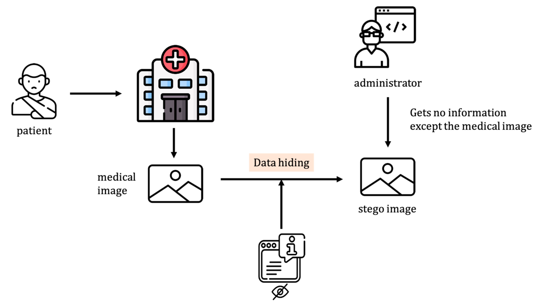
11]. In this work, the issue discussed is its application to medical images. In the hospital, a patient may take several kinds of medical images, and meanwhile, diagnosis data related to the patient are recorded on these images. However, if hospital database administrators access these images without proper authorization, the medical data may be leaked, and a “medical data breach” occurs. To meet the challenge, our scheme embeds data into a medical image. Since the medical image is distortion-sensitive, patients may be misdiagnosed due to subtle image changes. Therefore, we use RDH to recover the original image after the hidden data is extracted perfectly.
Figure 1 gives an overview of the proposed application scenario.
We categorize RDH methods into three domains: spatial domain, frequency domain, and compression domain. Most spatial domain methods embed data into the least significant bit (LSB) of a pixel in the image, providing good concealment performance. Since no additional transformation is required, the computational complexity is low, but related security and robustness are concerned. The frequency-domain method transforms the cover data into the frequency domain, for example by using Fourier transform. Then, hidden data are embedded in the frequency domain and converted back to the spatial domain. The advantage is that it has good robustness to the shearing attack, but it requires extra time for the transformation. RDH lies in the compressed domain, such as JPEG, decodes the JPEG-compressed image to get the original image first and then embeds the confidential data onto it. Finally, the image with the hidden data is encoded into JPEG format again. The disadvantage of this approach is that the performance is considerably related to the nature of the target image.
Most RDH techniques are applied to the spatial domain because of the intuitiveness of the algorithm and the low computational cost. Famous spatial domain RDH methods include difference expansion (DE), histogram shifting (HS), and LSB modification, to name a few.
Section 2 will give a discussion on RDH-related techniques in detail. Our proposed algorithm belongs to the branch of histogram shifting.
The contents of the following paragraphs are known to data hiding communities, but we include them for the article’s own completeness. According to the purposes of data hiding, the required characteristics include [
12]:
- (a)
Imperceptibility. After hiding the data, the cover data must maintain its original quality; moreover, the human sensory system cannot detect the embedded data (the most fundamental characteristic of data hiding).
- (b)
Undetectability. Embedded and cover data have very close statistical characteristics, such as noise distribution, entropy, etc. Even after benchmarked data analyses, an unauthorized receiver cannot know whether there is embedded information or not.
- (c)
Capacity: It is also called the embedding rate or effective payload, which is the maximum amount of information that we can embed in the host data.
- (d)
Efficiency: The processing time required to perform RDH defines the efficiency of the system.
However, it is difficult for any data hiding algorithm to consider all the characteristics mentioned above simultaneously because some of them are contradictory to one another. For example, to achieve a high capacity, we must modify the cover data greatly, leading to noise increasing and imperceptibility loss. Considering the characteristics of medical images, we mainly focus on capacity and imperceptibility.
Our Contributions
In this work, we design a novel fully reversible data hiding scheme that utilizes the smooth area of a medical image to embed data. We apply the proposed method to MRI images, CT images, and X-ray images. The contributions of this work are listed as follows.
- (a)
We present a novel two-bit embedding algorithm for RDH that uses medical images as inputs and achieves high capacity and less distortion.
- (b)
We propose a local complexity function suitable for our two-bit embedding algorithm to select which pixel is embedded. Results show that our algorithm embeds most of the hidden data in the RONI of medical images and causes less distortion in the ROI.
- (c)
Since there are many types of medical images, we used three common types, such as MRI, CT, X-ray, to verify the feasibility of our algorithm. Experiment results show that our algorithm achieves good performance and is suitable for these types of images.
2. Related Work
This section will review the techniques most relevant to RDH, steganography, and DW. Next, we will present several common approaches to conduct RDH.
2.1. Steganography and Digital Watermarking
- (a)
Steganography
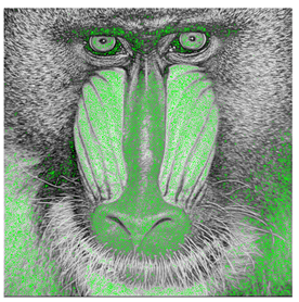
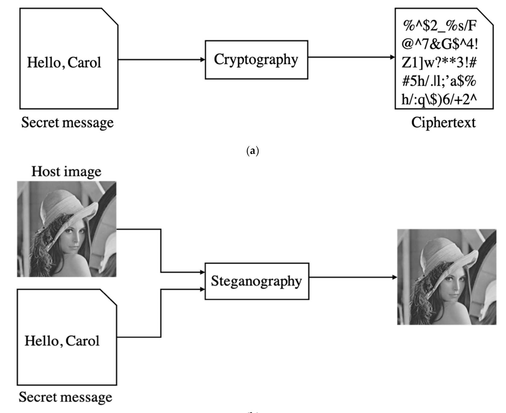
Steganography hides a secret message in cover data. The exact purpose of steganography and cryptography is to protect private messages. In cryptography, the hidden message after encryption is called ciphertext. In steganography, the cover image embedded with a secret message called the stegoimage. The main difference is that ciphertext looks like an error code (cf.
Figure 2a). After the attacker receives the encrypted message, he already knows there is a hidden secret. On the contrary, steganography makes attackers unable to detect the presence of a secret message (cf.
Figure 2b).
- (b)
Digital Watermarking.
DW is a branch of data hiding, and it also embeds data into cover media. The purposes of DW are protecting the copyrights of digital works, proving authenticity, piracy tracking, and so on. Therefore, DW hides specific information into digital work, such as author information, company trademarks, product numbers. According to the different scenarios, DW can be visible or invisible. Since others may illegally operate digital works, so the robustness of DW is the essential design factor.
Protecting confidential data is the primary purpose of steganography, while DW protects the cover data.
Table 1 shows the major differences between steganography and DW. This work aims to embed the information into medical images, which are related to patient privacy. Therefore, we utilized the steganography technique to implement RDH.
2.2. Approaches of Reversible Data Hiding
Before presenting the proposed framework, we address several state-of-the-art RDH algorithms first. These algorithms are LSB substitution, difference expansion (DE), histogram shifting (HS), and prediction error histogram.
2.2.1. LSB Substitution
LSB-substitution embeds the secret message into the LSBs of the target image’s pixels. Typical approaches include Wang [
13], Chan [
14], and Celik et al. [
15]. We describe the general operations of the LSB-substitution method below. For example, given a 3 × 3, eight-bit grayscale image, converting it into a binary representation, we obtain
| 01100110 | 01010101 | 01001011 |
| 11001011 | 10100010 | 01010111 |
| 11101110 | 11111101 | 00101010 |
Now suppose we want to embed the secret message 101100010 into the LSBs of this grayscale image. The following table shows the corresponding result, and the underlined bits of the table has been modified.
| 01100111 | 01010100 | 01001011 |
| 11001011 | 10100010 | 01010110 |
| 11101110 | 11111100 | 00101010 |
The advantage of this method is that the algorithm is intuitive, the distortion of the cover image is minor, and the introduced error is invisible. However, the hidden message may be lost through nearly any kind of image processing. That is, this method is not robust and vulnerable to minor attacks.
2.2.2. Difference Expansion (DE)
DE was proposed by Tian [
16] in 2003. The algorithm utilizes a pair of pixels
in a grayscale image and calculates the difference
. Then, the secret message will be hidden in the LSB of
. We describe the general operations of DE as follows. For example, we have a pair of pixels
Assume
, , and the hidden bit
. First, we calculate the average
and difference
of
and
. That is,
Next, we transfer the value
into its binary representation
. Then we append the hidden bit
to
, and get the new difference
.
Based on new value
and the average
, we calculate new value of pair of pixels
,
When we need to extract the hidden message, we compute the difference
and the average
. Then we can retrieve the hidden message based on the LSB of
. That is,
Finally, we can recover the original pair of pixels
The advantage of this method is that the algorithm is simple, and the capacity is high. According to the values of h’ in the algorithm, we will move the pixel values to both sides of the corresponding histogram, and the pixel value change is assumed uniform. However, the appending operation multiplies the difference value by two, which may cause significant distortion in the picture’s visual quality.
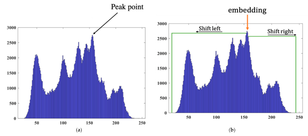
2.2.3. Histogram Shifting (HS)
HS was proposed by Ni et al. [
17] in 2006. The general operations of HS [
18,
19,
20] can be understood through the following simple example. First, we find the peak value point of the image histogram as shown in
Figure 3a.
Then the embedding function is defined as in Equation (1).
where
is the hidden bit and
is the peak value,
is the value of the original pixel, and
is value of the modified pixel. The realization of HS is illustrated in
Figure 3b.
The advantages of HS are its relatively high payload over that of the LSB-based approaches, and that the corresponding distortion is usually invisible. However, the peak point value of the histogram limits the embedding capacity of this method. The prediction error of adjacency pixels instead of the pixel value has been used to solve the above problem [
21,
22,
23]. Prediction-error-based methods significantly improve the capacity.
2.2.4. Prediction Error Histogram (PEH)
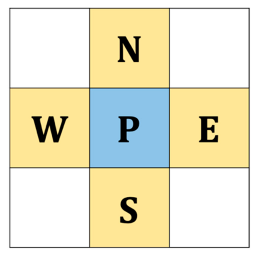
The original HS method has a limitation in the embedding capacity, which is dominated by the peak point value of the histogram. To deal with this problem, we transform the target image’s histogram into the prediction error domain to obtain the so-called prediction error histogram (PEH). First, we use four neighboring pixel values {
N, W, S, E} (cf.
Figure 4) to calculate the prediction value based on Equation (2):
Then, we compute the prediction error,
by using Equation (3):
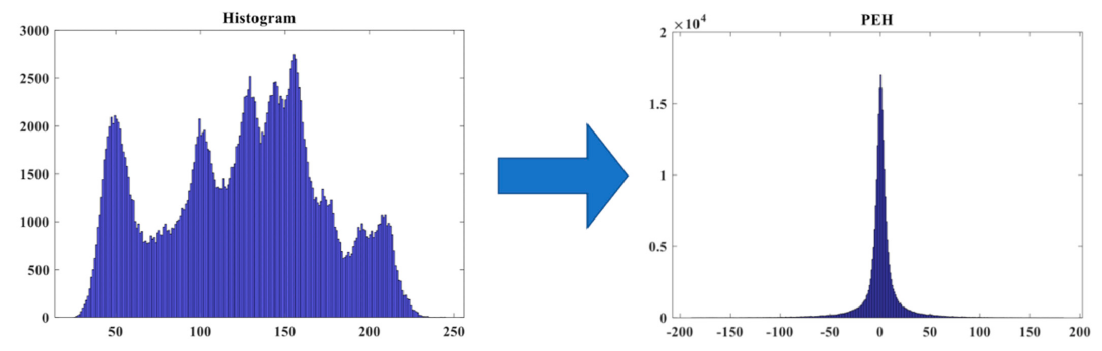
Finally, we generate the resulting PEH (see
Figure 5). As shown in the figure, the peak point gathers around the value of zero after doing the conversion. We are going to use this feature to embed the data in the zero-valued positions. More details of the algorithm will be described in the next section. Our proposed method utilizes PEH to implement the RDH, which will be detailed in
Section 3.
Steganalysis and steganography are the two different sides of the same coin. In other words, steganalysis attempts to defeat steganography by detecting hidden information and extracting or destroying it. Compression and encryption domains’ data hiding techniques have also attracted specific attention recently. However, we will not address them until the discussion section because they are out of the scope of this writeup.
3. The Proposed Method
Kim et al. proposed an RDH embedding method in [
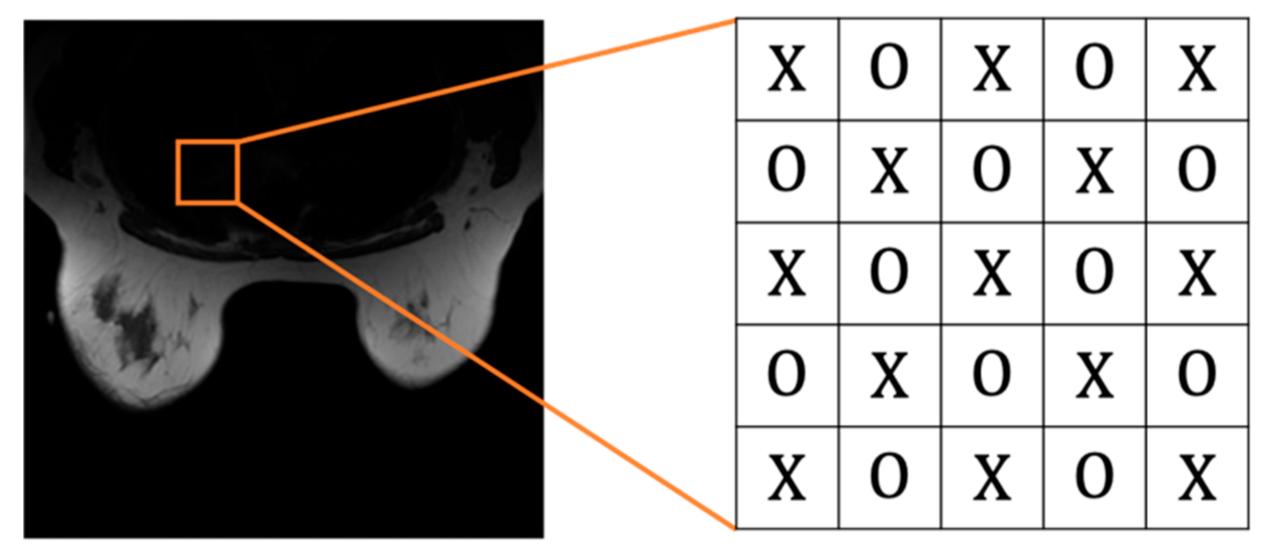
24], where pixels are divided into even and odd sets. If the sum of a pixel’s horizontal and vertical position indexes is an even number, it will be categorized into the even set. On the contrary, if the sum is an odd number, it will be organized into the odd set.
By extending Kim’s approach further, we present a new RDH framework in this work, which aims to embed the secret message into the smooth area of a medical image. We utilized a newly defined local complexity function to help to embed messages in the RONI. In addition, our method achieves high capacity and keeps the ROI almost unchanged.
3.1. Embedding Processes
Before embedding, we need to mention that medical images contain many pixels with zero value, so the pixels with zero value should be directly skipped during the embedding process. Our proposed scheme embeds messages in an even-and-odd version of embedding. First, we categorize pixels into even and odd sets (cf.
Figure 6). Pixels are categorized into an even set with an even-numbered sum in their horizontal and vertical position indexes and an odd set vice versa. Note that the two sets are independent. Therefore, once the pixel in one group is modified, it won’t affect the other set. We can use this property to compute prediction values. The proposed algorithm is divided into two rounds, so each pixel is embedded twice through the algorithm. Before performing our algorithm, we convert the hidden data into binary.
In the first round, the prediction error is
, and we embed one message bit in
based on the following Equation:
where
is the stegopixel, and
is the embedded message bit in the first round. The message bit will be embedded only when the prediction error is 0, which means that
has the same value as the average of its surrounding pixels. When the prediction error is strictly positive, we increase the values of the corresponding pixels by 1 and keep other pixels unchanged.
In the second round, the prediction error becomes
, and we embed one more message bit in
based on the following equation:
where
is the stegopixel with two bits embedded, and
is the embedded message bit in the second round. Again, the message bit will be embedded only when the prediction error
is 0, which means that value of
is the same as the average of its surrounding pixels. When prediction error is strictly negative, we will decrease the values of the corresponding pixels by one and keep other pixels unchanged.
Note that a RONI is a relatively smooth region in the whole image, and this feature founds our algorithm. Therefore, we prefer to keep the pixels in ROI unchanged. An embedding example in a smooth area is illustrated in
Figure 7. The main advantage of our algorithm is its ability of two-bit embedding in one pixel.
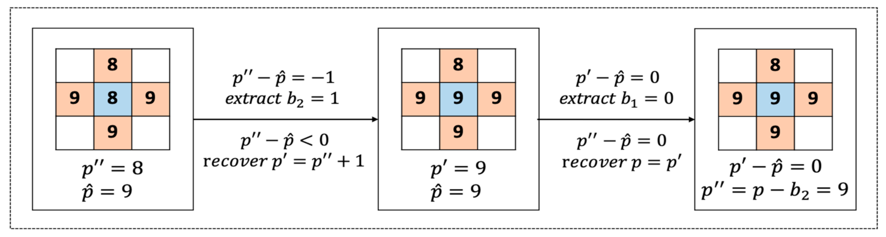
3.2. Extraction and Recovery Processes
In this subsection, we present how to extract the hidden data and recover the original image. Since the pixels with zero value have been skipped during the embedding process, similarly, in the process of extraction and recovery, pixels with zero value will be ignored, too. Extraction and retrieval processes are done in reverse order of that of the embedding. That is, we will recover the odd set first, then the even set. Embedded message bit
in the second round is extracted by Equation (6):
Recovery of
in the second round is done based on the following equation:
After the second round is completed, the embedded message bit
in the first round is extracted based on the following equation:
Then, recovery of
in the second round can be done by the following function:
An example of the proposed two-bit extraction and recovery is illustrated in
Figure 8.
Finally, the even set is recovered and extracted by repeating the same steps. The embedding order of each pixel in one set depends on its local complexity function, which will be described in the next section.
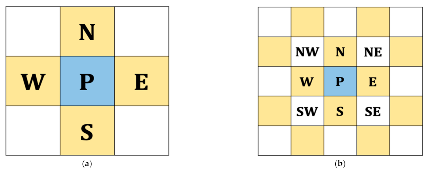
3.3. The Local Complexity Function
As described above, RONI is relatively smooth compared to ROI, and we utilize this feature to select pixels that should be embedded first. We designed a local complexity function to deal with pixel selection to reduce the distortion in ROI. The main idea is to calculate how smooth a pixel is when surrounded by the defined neighboring pixels. Note that the smaller the value of local complexity, the more likely it is a smooth pixel, which is more embeddable. Therefore, pixels with a smaller value of local complexity are embedded first. The four-pixel version of the local complexity function is exploited (cf.
Figure 9a) in the following. We use an extended version that can select a smooth area more precisely.
As shown in
Figure 9a, we use four neighboring pixels to compute the four-pixel version value
based on the following equation:
Figure 9b shows the context of our proposed extended version. The following function describes the above-mentioned extension:
3.4. The Proposed Encoder and Decoder
In this subsection, we present the proposed encoder and decoder. In addition, the involved side information will be comprehensively discussed as follows.
3.4.1. Side Information of the Decoder
The proposed decoder needs certain side information to extract the embedded message and recover the stegoimage to the original one. The following subsection describes the side information related to the decoder.
- (a)
The Location Map
In order to avoid the overflow problem, we need to preprocess some pixels and record them in a location map. For a 16-bit medical image, the maximum pixel value is 65,535. However, in embedding, the pixel value may be modified, which causes the pixel value to be shifted to 65,536. Therefore, we have to preprocess the pixel value to avoid the overflow problem. However, suppose a pixel with value one has been moved to zero after embedding; it will be skipped during the recovery and extraction. Accordingly, we need to move the pixels with values from 1 to 2 and record them on the location map before embedding. Without loss of generality, we assume k pixels have been preprocessed. The location map
is generated and the original pixel
is preprocessed to obtain
based on the following equations:
We use the arithmetic code to losslessly compress the location map and append the result to the front of the hidden data. Given an
image, the size of the location map
bits. That is, for a 512 × 512 image, the size
is 18 bits. Then, in our recovery stage, the original pixel
is recovered from
using the location map
based on the following equation:
- (b)
Hidden Message Length
To know when to stop decoding during the decoding process, we must record the hidden message length on the LSBs of the border pixels. That is, we replace the LSBs of the border pixels with the associated hidden message. In addition, we have to append these border pixels to the front of the hidden message to recover the corresponding pixels in the decoding process correctly. Given an image, the size of hidden message length is bits. That is, for a 512 × 512 image, the size is 18 bits.
- (c)
The LSBs of the Border Pixels
The hidden message length is recorded at the LSBs of the border pixels, so we need to append LSB bits of the border pixels to the front of the hidden message and use them for the recovery process.
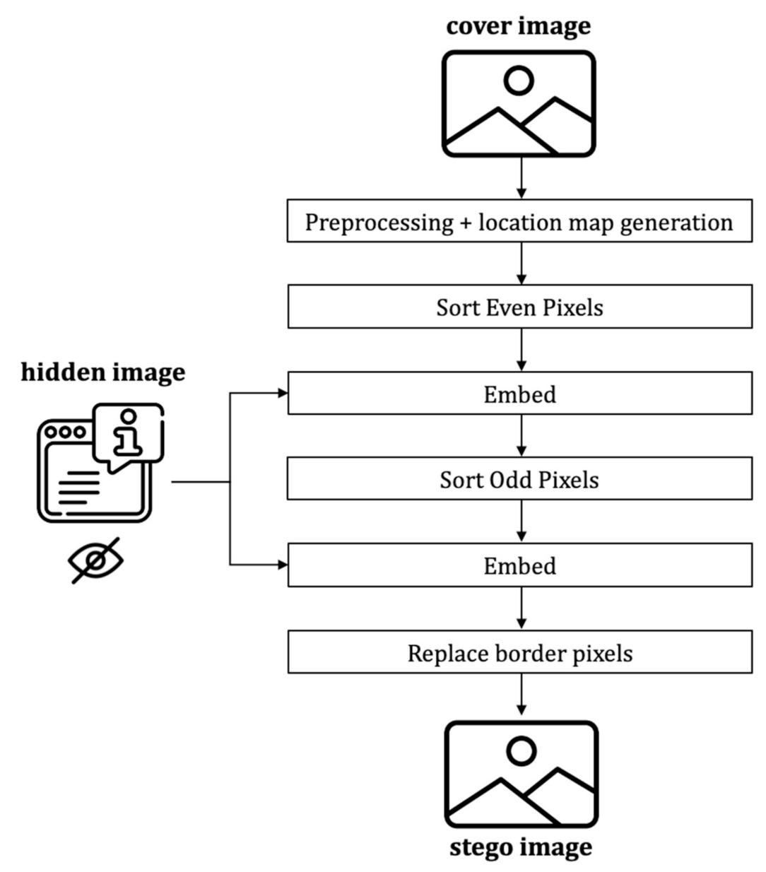
3.4.2. The Encoding Process
The encoding process includes the message embedding, which follows the following steps (cf.
Figure 10):
Preprocess and generate location map
Sort even set pixels based on the proposed extended version of the local complexity function.
Embed hidden message in the even set.
Sort odd set pixels using the proposed extended version of the local complexity function.
Embed hidden message into the odd set.
Replace the border pixels.
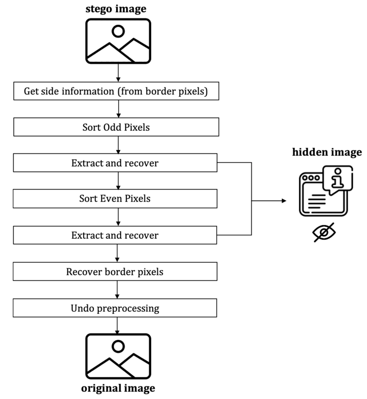
3.4.3. The Decoding Process
The decoding process includes the hidden message’s extraction and the recovering of the original image, which follows the following steps (cf.
Figure 11):
Get side information from LSBs of border pixels.
Sort odd set pixels using the proposed extended version of the local complexity function.
Extract hidden messages and recover pixels in the odd set.
Sort even set pixels using the proposed extended version of the local complexity function.
Extract the hidden message and recover the pixels in the even set.
Replace LSBs of the border pixels with the original LSBs
Decompress the location map and undo the associated preprocessing.
4. Experimental Results
We have comprehensively addressed the proposed RDH scheme in
Section 3. This section compares our method with other related approaches by performing experiments on several medical image databases. To verify the flexibility of our method, we also execute the proposed process in public image databases. First, we introduce the databases we used, including medical images and general images. Next, the evaluation metric that these databases applied will be described. After that, the experimental results will be shown and compared with other state-of-the-art methods.
4.1. The Tested Databases
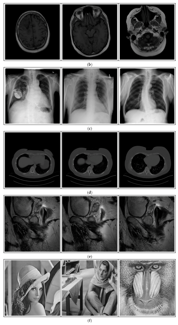
This section introduces the databases used in our experiments, including medical images and general images. As suggested by one of the anonymous reviewers, the web addresses of the involved testing databases are provided for readers’ ease of reference. The details of these databases are as follows.
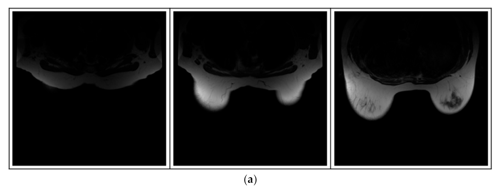
- (a)
Breast-MRI-NACT-Pilot is an MRI-type image database, collecting breast medical images of 64 patients. Some samples are shown in
Figure 12a.
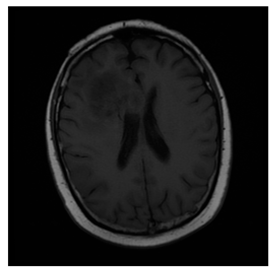
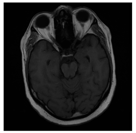
- (b)
ACRIN-DSC-MR-Brain database contains MRI-type and CT-type brain medical images. Some samples are shown in
Figure 12b.
- (c)
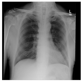
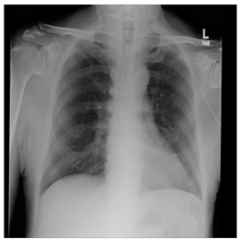
NIH Database
ANIH is an X-ray type image database collecting chest medical images. Some samples are shown in
Figure 12c.
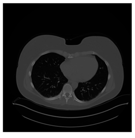
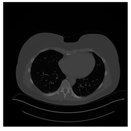
- (d)
Lung-PET-CT-Dx is a CT-type image database collecting lung medical images. Some samples are shown in
Figure 12d.
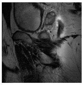
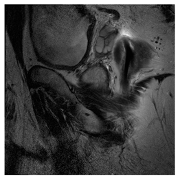
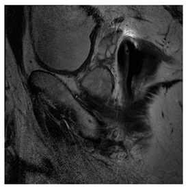
- (e)
Prostate-MRI database contains MRI-type medical images and collects prostate medical images. Some samples are shown in
Figure 12e.
- (f)
Other grayscale standard images
In order to investigate the flexibility of our method, we also tested several available images, as shown in
Figure 12f.
4.2. The Evaluation Metrics
Since this work focuses on medical images, we aim to achieve high capacity and imperceptibility, and the following evaluation metrics are used to verify our algorithm.
- (i)
Capacity: We measure the maximum amount of data that can be embedded in a tested medical image.
- (ii)
Peak signal-to-noise ratio (PSNR): PSNR is the most common and widely used objective measurement for image quality assessment defined by mean square error (MSE). Given an 𝑚 × 𝑛 reference image 𝐼 and a noisy image 𝐾, MSE is defined as Equation (15):
and PSNR is defined as Equation (16):
where
is the square of the maximum pixel value of the image.
However, according to many experimental results, the PSNR score cannot precisely match the human vision system (HVS), so we also use an objective quality measurement method, SIM, mentioned below, to make the experiment more complete.
- (iii)
Structural similarity index measure (SSIM)
The basic idea of SSIM is to evaluate the similarity of two images
x,
y, through the luminance (
l), contrast (
c), and structure (
s) defined as Equations (17)–(19):
is the average of
x, and
is the average of
y.
is the variance of
x, and
is the variance of y.
is the covariance of
x and
y.
,
, and
are constants to avoid dividing by zero. Then, SSIM is defined as Equation (20):
According to many experimental results, the evaluation performance of SSIM is closer to the human visual system than PSNR. We implemented the above three metrics to compare our experimental results with those of other works.
Notice that the perceptibility of image details depends on the sampling density of the image signal, the distance from the image plane to the observer, and the perceptual capability of the observer’s visual system. In practice, the subjective evaluation of a given image varies when these factors change. A single-scale method, such as SSIM, may be appropriate only for cases with a specific setting. Since the multiscale approach in the image quality assessment community is a way to incorporate image details at different resolutions, Wang et al. proposed the multiscale version SSIM (called MS-SSIM) as a better image quality assessment metric. In MS-SSIM, with the reference and distorted image signals as the input, the system iteratively applies a low-pass filter and downsamples the filtered image by a factor of two. Then, indexing the conventional single-scale SSIM (SS-SSIM) as in Scale 1 and the highest scale as in Scale M, obtained after M − 1 iterations. The overall MS-SSIM evaluation is obtained by combining the SS-SSIM measurements at different scales with relative importance weights, which would be empirically determined. That is, paying a certain amount of computational overhead could better the subjective image quality measurement.
Since our task targets RDH in medical images, we mainly focus on imperceptibility and capacity. PSNR and SSIM are used to analyze the corresponding performance. We did not take MS-SSIM into account because it is not widely adopted in RDH in medical image related works; moreover, we have to do many experiments to find the appropriate parameter settings. As we mentioned in
Section 3, we use the proposed local complexity function to select which pixel is embedded first, so we should carefully consider the positions of the modified pixels.
4.3. The Results
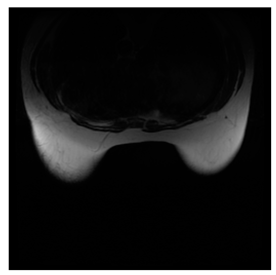
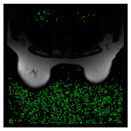
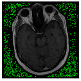
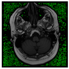
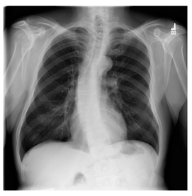
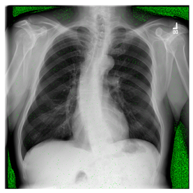
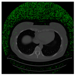
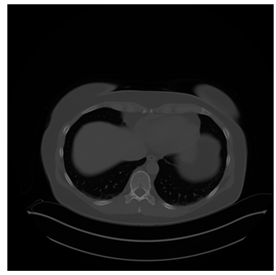
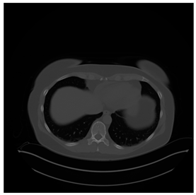
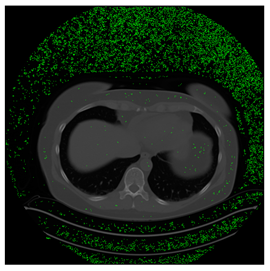
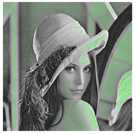
In this subsection, we describe three experiments used to measure the performance of the proposed method. The first experiment shows the stegoimage and marks the pixels’ positions that have been modified during the embedding process, as shown in
Table 2,
Table 3,
Table 4,
Table 5,
Table 6 and
Table 7. To make modified pixel positions have a pronounced effect, we set bpp (bit per pixel) rate at 0.05 and 0.025. It can be seen from the results that the proposed local complexity function can distinguish ROI and RONI from most of the medical images, so modified pixels are mainly gathered in RONI. However, it is observed that the proposed local complexity function cannot distinguish between ROI and RONI in the Prostate-MRI database due to the relative complexity of the image. Besides, “Modified BPP” represents the proportion of pixels in the image that have been modified. We observed that the performance of “baboon” in the grayscale standard images database is poor because that image’s pixels are relatively complex. It becomes challenging to select the more embeddable pixels based on the proposed local complexity function. Nevertheless, the modified pixel positions in other grayscale standard images, such as Lena and Barbara, are relatively smooth, verifying that our local complexity function is also applicable to general images.
Next, our second experiment tested the Breast-MRI-NACT-Pilot database, the ACRIN-DSC-MR-Brain database, and the NIH database and compared the associated maximal capacity with other methods, as shown in
Table 8. The method proposed by Kim et al. is also histogram-based, and the difference from our approach is in the embedding algorithm and the adopted local complexity function. Li’s method was proposed earlier, which is also a histogram-based method, but it didn’t use prediction error and local complexity function. Therefore, our performance is significantly better than theirs. We can observe that better maximal capacity is achieved in the NIH database. This better performance comes from the fact that the image size of the NIH database is 1024
1024; however, the image size of other databases is 256
256.
The last experiment was under the condition of a fixed bpp rate. As shown in
Table 5,
Table 6,
Table 7,
Table 8 and
Table 9, we compared the performances about the number of the modified pixels, PSNR, and SSIM. The results show that our method performed better than others. Note that the maximal capacity of Li’s method cannot reach 0.05 bpp on several tested databases, so we didn’t include it in our comparison.
5. Conclusions
In practice, patients’ medical images are examined by doctors to check or identify for assistance in the diagnosis. The image distortion or quality degradation caused by data hiding may cause serious problems, and therefore, should be avoided as much as possible. Moreover, any loss in the restored information is not acceptable. On the other hand, much examination-related metadata should be recorded and restored associated with medical images during the diagnosis. Therefore, unlike general images, reversibility and high-capacity are on the top of the requirement list for data hiding in medical images. In this paper, we proposed a novel two-bit embedding architecture for data hiding. In contrast to most of the existing data hiding approaches, our work is fully reversible. To the best of our knowledge, we are the first to use the local complexity function to divide a medical image into smooth and unsmooth areas. Our embedding algorithm causes less distortion in ROI. Furthermore, the experimental snapshots show that the hidden message embedded in the stegoimage is invisible.
Besides DW and steganography, another way to protect sensitive image data is to transfer all data and associated processing to the encryption domain using appropriate cryptographic mechanisms. This branch of researches leads to the development of massive amounts of RDH schemes in encryption image (RDHS-EI) [
24,
25,
26,
27,
28,
29,
30]. Similar to RDH, RDHS-EI targets to embed additional confidential data into the encrypted image without destroying the carrier image. That is, the embedded sensitive data must not affect the accuracy of the recovered carrier image decrypted from the encrypted domain.
As described in
Section 2, the abilities to survive steganalysis and hide data in the compression and the encryption domains are not considered in this writeup yet. According to the excellent and thorough classification of recently published 24 RDH-in-the-encrypted-image (RDH-EI)-related papers presented in [
31], the existing RDH-EI schemes [
31] and the references therein] can be classified into the following three categories: vacating room after encryption (VRAE), reserving room before encryption (RRBE), and vacating room by encryption (VRBE). Notice that, according to the illustrated frameworks Figure 1 in [
31], traditional RDH approaches (including LSB modification, DE, HS, and the one presented in this work) can still play the pivotal role of data embedding besides various adopted encryption steps. Intuitively, however, to realize data hiding in the encryption domain, we must encrypt the carrier image first and then find redundant space in the encrypted image to embed additional data. Nonetheless, generating a sizeable redundant space in the encrypted image is challenging because, in theory, an effective encryption process will completely destroy the correlation among image pixels. As noted in [
31], this is the main reason for the low embedding rates of the VRAE, RRBE methods. Fortunately, [
31] proposed an interesting two-tuples coding method to represent the carrier image which can reserve an ample redundancy space in the encrypted images for embedding extra data. That means, combining the two-tuples coding and our two-bit embedding method, we may increase the embedding capacity of RDH methods in the encryption domain also. Of course, we need to conduct a series of experiments to justify the associated performance, which is definitely one of our future works.
Finally, as one of the anonymous reviewers suggested,
Table 10 summarizes the advantages and disadvantages of data hiding algorithms for medical Images mentioned in this work. As pointed by the academic editor that the SSIM values presented in
Table 9 only differ in the third decimal digit, which suggests that SSIM doesn’t seem to provide that much information to the image quality evaluation (cf. the “distortions in ROIs” column). For comparison, as suggested by the academic editor, we include the SSIM specific to ROIN (denoted as SSIM-ROIN) in the last column of
Table 9. However, SSIM is an index used to analyze the similarity of the image structure. Our modification to the pixel value is plus or minus 1; the whole image structure does not change much, so the SSIM calculated precisely for RONI won’t be different from the entire image counterpart too much. On the one hand, this observation coincides with our conclusive summary presented in
Table 10; on the other hand, a better performance index, such as MS-SSIM, may be used instead. This task is, of course, one for future research works. The inferior timing performance of the proposed approach compared with Kim’s and Li’s methods comes from the following extra overheads: (1) the computation of the local complexity function for selecting embedding positions and (2) the computation of the side-information for correct decoding. Fortunately, according to our experiments, we can accomplish all the computations within seconds in time, even for a 1024 × 1024 X-ray image in the NIH dataset. Besides the RDH schemes in the encrypted domain, in the future, we will develop an algorithm that resists JPEG compression to improve the robustness. In addition, we will further compare other prediction methods such as the block-based approaches and include steganalysis into our process to justify the corresponding practical value of the algorithm.


