Abstract
The problem of the optimal reactive power flow in transmission systems is addressed in this research from the point of view of combinatorial optimization. A discrete-continuous version of the Chu & Beasley genetic algorithm (CBGA) is proposed to model continuous variables such as voltage outputs in generators and reactive power injection in capacitor banks, as well as binary variables such as tap positions in transformers. The minimization of the total power losses is considered as the objective performance indicator. The main contribution in this research corresponds to the implementation of the CBGA in the DigSILENT Programming Language (DPL), which exploits the advantages of the power flow tool at a low computational effort. The solution of the optimal reactive power flow problem in power systems is a key task since the efficiency and secure operation of the whole electrical system depend on the adequate distribution of the reactive power in generators, transformers, shunt compensators, and transmission lines. To provide an efficient optimization tool for academics and power system operators, this paper selects the DigSILENT software, since this is widely used for power systems for industries and researchers. Numerical results in three IEEE test feeders composed of 6, 14, and 39 buses demonstrate the efficiency of the proposed CBGA in the DPL environment from DigSILENT to reduce the total grid power losses (between 21.17% to 37.62% of the benchmark case) considering four simulation scenarios regarding voltage regulation bounds and slack voltage outputs. In addition, the total processing times for the IEEE 6-, 14-, and 39-bus systems were s, s, and s, which confirms the low computational effort of the optimization methods directly implemented in the DPL environment.
1. Introduction
Electric power systems in high-voltage levels are electrical networks with the responsibility of transporting large amounts of energy from generation plants to sub-transmission and distribution substations [1]. These grids are typically composed by transmission lines that cover hundreds of kilometers of territory and these are typically operated at voltage levels larger than 220 kV [2]; to compensate possible voltage swell and overvoltages produced by load variations reactive power compensators are integrated on these grids based on capacitor and reactor banks, which operate in steps of injection as a function of the grid requirements [3,4]. In addition, to control the voltage profiles along the grid the tap changers are also used in transformers and the voltage controllers in the synchronous machines [5]. These devices must be properly coordinated to support voltage and frequency for all possible operative conditions of the network [6]; however, these are not easy tasks as specialized control and optimization methodologies are required [1].
An additional aspect in the operation of the power systems under steady state conditions corresponds to the admissible power losses in the normal operation of the network [7], since the energy losses can be reduced with the adequate operation of the taps in transformers, capacitor and reactive power compensators as well as the voltage controllers in the synchronous machines [5]. To represent the problem of power losses minimization in power systems it is required the formulation of an optimization problem that has a mixed-integer nonlinear programming (i.e., MINLP) structure, where efficient and easily implementable optimization strategies to solve it are needed.
In the specialized literature multiple approaches have been proposed to solve the aforementioned problem which is widely known as the optimal reactive power flow problem based on combinatorial optimization methods. Some of these methodologies are described below.
Authors of [8] have presented a multi-objective model to represent the problem of the optimal reactive power flow in power systems where the energy production costs and the total grid energy losses are considered as conflict objectives. The proposed MINLP formulation is solved through the -constrained method through the General Algebraic Modeling System (i.e., GAMS) software. Numerical results demonstrate the effectiveness of the proposed methodology in IEEE test systems composed of 14 and 30 buses, when compared with metaheuristic optimizers such as particle swarm optimization, and differential evolution algorithm, among others. Authors in [9] proposed a specialized metaheuristic optimization algorithm to deal with the optimal reactive power flow problem in power systems which is named stochastic fractal search method. In the objective function it is considered the minimization of the grid energy losses, the voltage deviation, and the voltage stability index. Londoño et al., in [6] presented the application of the mean-variance mapping optimization algorithm to the optimal reactive power flow problem. The effectiveness and robustness of the proposed algorithm is tested in the IEEE 30-bus system, and compared with multiple metaheurisitic optimizers. These comparisons demonstrated that the proposed algorithm reaches the minimum power losses for this system with the best numerical convergence of 10 comparative methodologies. Authors in [10] presents a comparison of three optimization methods to address the reactive power solution in power systems composed of 6, 14 and 39 bus systems. These algorithms correspond to the particle swarm and genetic algorithms improved with the pattern search optimization algorithm. Numerical results demonstrated the effectiveness of the proposed optimization approaches; however, the authors do not provide enough information to corroborate their results, additionally, the variables were codified using continuous approximations, which can affect the final solution based on the integrity and feasibility of the solution space. Authors in [11] have proposed a novel fuzzy adaptive heterogeneous comprehensive-learning based particle swarm optimization algorithm with enhanced exploration and exploitation processes to solve the optimal reactive power dispatch problem in large-scale transmission systems. Numerical validations were performed in power systems with sizes within 30 to 354 nodes, and their results improved the solutions reached with the classical Particle swarm optimization algorithm. In [12] it is presented a complete revision regarding the optimal reactive power flow problem in transmission systems. In addition, the authors have proposed the application of the sine-cosine algorithm to solve this problem with tests instances of 14, 30 and 57 nodes, respectively. The main contribution of these authors corresponds to the statistical validation of the the proposed sine-cosine algorithm when compared with other metaheuristics such as differential evolution and particle swarm optimization, among others. Zhao et al. in [13] presented an interesting work regarding the optimal power flow problem considering the intrinsic relation between the transmission and the distribution networks. The main contribution of this approach corresponds to the proposition of the a distributed gradient-based optimization algorithm to solve the optimal reactive power flow problem considering dispersed distributed generation in distribution networks.
Some additional optimization techniques applied to reactive power flow problem in power systems are: particle swarm optimization [14,15,16,17,18]; gravitational search algorithm [19,20]; moth-flame optimization technique [21]; differential evolution algorithm [22]; bat optimization algorithm [23]; genetic algorithms [5,8,24]; tabu search algorithms [25,26]; and slime mold algorithm [27], among others
Unlike the previous reported approaches, in this research the purpose is the implementation of a specialized genetic algorithm in the DigSILENT programming language (DPL) to set all the variables associated with the optimal reactive power flow problem. The main advantage of the proposed optimization method corresponds to the usage of the well known power flow tools in the DigSILENT software [28]. In addition, this software allows to model the complete power system as much as possible with synchronous machines, two- and three-winding transformers, capacitive and reactive compensators and models of complete line [29]. The validation of the proposed optimization approach is carried out in three different power systems composed of 6, 14 and 39 nodes, respectively, which present prominent numerical results. An important fact of our proposed optimization approach is that the genetic algorithm that solves the optimization problem combines binary and discrete variables in a unified codification [30]. This codification make possible to solve the integer and continuous part of the exact MINLP model in one step, which reduces the complexity of the optimization tool and decreases the total processing time required in its solution. In addition, to guarantee the repeatability of our results, all the DigSILENT systems with the optimization codes are provided into a free repository to allow future research developments.
It is worth mentioning that the DigSILENT software has been selected for all the numerical implementations based on the following criteria:
- ✓
- It has an embedded programming language that uses the power system interface to evaluate multiple power flows with minimum computational requirements.
- ✓
- The DigSILENT software allows the detailed modeling of the power system components such as transformers, reactors, transmission lines, generators and induction motors, among others. These are easily integrated in power flow studies through the Newton-Raphson approach.
- ✓
- The DPL tool avoids to use external programming interfaces to implement the optimization codes; which reduces the total computational time of the optimization strategy.
In addition, it is important to mention that the main goal with this contribution is to provide an efficient and reliable optimization technique (also classical and well-known as the case of CBGA) that can be easily adapted for power system operators as part of their analysis tools [31,32]. However, due to the recent advances in optimization techniques, it becomes quite interesting to implement the solution strategies based on artificial intelligence for future works [11].
The remainder parts of this document are rearranged as follows: Section 2 presents the general mathematical formulation of the optimal reactive power flow problem in power systems; Section 3 presents the main aspects of the solution methodology based on the implementation of a discrete-continuous version of the CBGA. Section 4 presents a general description of the DPL environment from DigSILENT. Section 5 shows the main features of the IEEE bus systems which are composed of 6, 14 and 39 buses, respectively. Section 6 presents all the computation validations for these test systems, considering four simulation scenarios associated with the voltage output at the slack node and the lower and upper voltage bounds. Finally, Section 7 lists the concluding remarks and possible future works derived from this study.
2. Mathematical Model
The problem of the optimal reactive power dispatch in power systems is a complex MINLP model, where the continuous variables are associated with the voltage magnitudes and angles, and active and reactive power generations, among others; while the integer variables are mainly associated with the tap positions in transformers, and active and reactive power compensators. The complete optimization model considered in this research is described below.
2.1. Objective Function
The typical objective function regarding associated with the problem of the optimal reactive power flow problem corresponds to the minimization of the total grid power losses for a particular load operation scenario. This objective function can be formulated as follows:
where corresponds to the value of the objective function associated with the grid power losses; and represent the voltage magnitudes in the k and m nodes, respectively, which have angles and , respectively; is the magnitude of the admittance that relates nodes k and w which is a function of the transformer taps . This admittance has an angle . Note that these values are obtained from the nodal admittance matrix. In addition, represents the set that contains all the grid nodes.
It is worth mentioning that the admittance matrix that relates all the nodes of the system is a nonlinear function of the tap positions in all the transformers, since these devices modify the operative state of the transformer by adding capacities and inductive effects on it, which produce modifications on the reactance components of the admittance matrix between the nodes when the transformers are connected [33].
2.2. Set of Constraints
The set of constraints of the reactive power flow problem includes the active and reactive power balance equations, tap in reactive power compensators and generation capabilities, among others. The complete list of constraints in the reactive power flow problem is presented below [10].
where and represent the active and reactive power injections provided by the generator connected at node k; and are the active and reactive power consumptions in the node k by the constant power loads; represents the reactive power injection by a capacitor bank connected at node k with the tap position ; represents the reactive power absorption by a reactor connected at node k with the tap position ; is the output voltage for a generator i; tap position for the capacitor bank; tap position for the reactor compensator; and represent the lower and upper bounds associated with the voltage variables in the generation nodes; and are the lower and upper reactive power generation bounds for a generator connected at node k; and are the minimum and maximum bounds allowed for the tap position in the capacitor bank; and are the minimum and maximum bounds allowed for the tap position in the reactor; and are the minimum and maximum bounds allowed for the tap position in the transformer; and and represents the lower and upper voltage regulation bounds applied to the node.
It is worth mentioning that the reactive power injection in the capacitor banks or the reactive power absorption in the reactors is a function of the tap position in these devices [6,34]. In addition, depending on the nature of the tap modeling, these can be represented as continuous variables (ideal case) or with discrete stages (real case), where the former produces a nonlinear optimization model, and the latter a general MINLP problem [35].
2.3. Interpretation of the Mathematical Model
The interpretation of the mathematical model (1)–(9) is described as follows: Equation (1) defines the objective function of the optimization problem which is related with the total grid power losses for a particular load condition. Equation (2) defines the active power balance in all the nodes of the network, and Equation (3) defines the reactive power balance in all the buses of the system. Inequality constraints (4) and (5) define the voltage and reactive power generation bounds in all the generators connected to the power system. Constraints (6) to (8) guarantees that all the taps in capacitor banks, reactors and power transformers are within their bounds; finally, inequality constraint (9) ensures that the voltage regulation bounds in all the nodes of the network stay within of their maximum and minimum allowed bounds.
The main complication of the optimization problem (1)–(9) is associated with the non-convexity of the solution space mainly caused by the active and reactive power balance constraints and the nonlinear dependence of the admittance matrix with the transformer taps [9,36]. Additional to these complications, the presence of the integer variables that generate disconnections in the solution space, make necessary to propose efficient optimization techniques that ensure adequate solution with low computational requirements, even when these are sub-optimal solutions.
3. Solution Methodology
To solve the problem of the optimal reactive power flow in power systems, represented through the optimization model (1)–(9), in this research, we propose the implementation of the well-known CBGA in the DPL by combining discrete and continuous codifications in a unique solution vector. The main advantage of the proposed approach corresponds to the usage of the additional power system analysis tools in the DigSILENT software as is the case of the power flow solution via the Newton-Raphson method. Figure 1 presents the main aspects of the implementation of a CBGA to solve optimization problems.
Figure 1.
General flow diagram for the implementation of a CBGA in optimization problems: (A) Initial population, (B) selection operator, (C) recombination operator, (D) mutation operator, (E) mutated individuals, (F) selection of the winner individual, and (G) inclusion of the winner individual in the current population.
Note that the implementation of the CBGA depicted in Figure 1 is composed of 7 main aspects tagged with A to G letters. Here, we highlight each one of these aspects.
- Section A: In this step it is formed the initial population of the CBGA which corresponds to a generation of multiple random solutions that fulfills the nature and upper and lower bounds of the decision variables. Then, each one of these solutions is evaluated in the power flow tool of the DigSILENT software and ordered in ascending form based on their power losses. Then, the first N individuals are selected as the reduced initial population. Note that this individual in the current population must be different to fulfill the diversity criterion of the CBGA.
- Sections B, C, D and E: In these sections are applied the selection, recombination, and mutation operators of the CBGA, where the main characteristic is that the parents selected must be different. These are randomly selected from the current population. Note that once the mutation operator is applied, to preserve the feasibility of its descending individual, the upper and lower bounds of the decision variables are revised and corrected if necessary.
- Sections F: In this stage, both descending individuals are evaluated in the power flow tool in the DigSILENT software to determine the power losses reached by each one of these configurations.
- Sections G: Finally, in this stage, the best descending is selected (i.e., the winner son) to evaluate the possibility of including it in the current population. To decide whether or not this individual is inserted into the current population, two aspects are revised: (i) the winner individual is different from all the parents in the population; and (ii) the objective function of the winner individual is better than the worst individual in the population. If both criteria are met, then, the current population is updated with the winner individual.
Remark 1.
Note that the evaluative process of the CBGA illustrated in Figure 1 returns from Section G to Section B, while the maximum number of iterations assigned for the exploration and exploitation of the solution space has not been reached.
To illustrate the general structure of a solution individual applied to the problem of the optimal reactive power dispatch in power systems, in (10) the proposed codification is presented.
Note that in this codification, the first positions corresponds to the decision variables associated with the voltage output in all the generators, the second part of the vector is composed by positions that are related with the tap positions in all the transformers; the third part of the codification is associated with the positions related with the capacitor taps, and the fourth part of the codification is associated with the positions related with the reactor taps; respectively.
4. DigSILENT Programming Language
The DigSILENT software is a power system analysis tool where static and dynamic analyses can be developed from high- to low-voltage AC networks, including direct current applications [37]. This is a widely recognized software used by power system industries, universities and research facilities to analyze electrical networks, being the main advantage that most of the components of these systems can be modeled with a high-level of precision [38]. In this research is used the DigSILENT software to model the three IEEE power systems under study; in addition, one of its main tool, i.e., the Digsilent Programming Language, is used to implement the proposed CBGA.
The main advantage of using DPLs in the DigSILENT software is that uses its own DigSILENT objects to evaluate the electrical performance of the electrical network with low computational effort [29]. The DPL is, in general, a structured programming language embedded in the DigSILENT software that permits call iteratively its different DigSILENT power system tools, e.g., balance and unbalanced power flow tool or stability analysis tool, to propose efficient algorithms that improve some objective performance indicators such as power and energy losses or stability indexes [39], among others.
In this research, the DPL environment is used to implement the CBGA to solve the reactive power flow problem in transmission systems by using recursively the Newton-Raphson power flow tool available in the DigSILENT software [29]. To illustrate a small DPL implementation, the power flow tool is called in the DPL for the IEEE 6-bus system (this system is presented in detail in the following section) to determine the total power losses of the network and report in the output window as can be seen in Figure 2.
Figure 2.
Example of a DPL in the DigSILENT software to evaluate the Newton-Raphson power flow and report the total grid power losses.
It is worth mentioning that to implement the power flow evaluation presented in Figure 2 it is necessary to know about the DPL syntax and possible embedded functions as the case of the FLUJO.execute(), where the word “FLUJO” is a word define by the programmer that is related with the power flow object in the DigSILENT programming tool selection.
For complete details regarding the usage of the DPL environment from DigSILENT, references [29,40] are recommended.
5. Power Systems under Study
In this section are presented the main characteristics of the power test systems under study, being these composed of 6, 14, and 39 nodes, respectively. Note that the latter two systems can be found directly in the DigSILENT test systems; however, to allow future validation of the proposed approach, here, we describe in detail each one of these test systems.
5.1. IEEE 6-Bus System
The electrical configuration of the IEEE 6-bus system is depicted in Figure 3. This system corresponds to a meshed transmission system composed of 5 transmission lines, 2 power transformers, 2 power generators (including the slack node), and 2 capacitive banks. The main characteristics of these devices is listed in Table 1.
Figure 3.
Electrical configuration of the IEEE 6-bus system.

Table 1.
Main parameters for the IEEE 6-bus system.
Note that in Table 1 were reported all the nominal parameters of the generators, transformers, capacitor banks and loads associated with the IEEE 6-bus system. Note that in the case of the capacitor banks these are modeled with synchronous compensators (see Figure 3) with nominal capabilities of reactive power generation from 0 to 5 Mvar.
Table 2 presents the main characteristics of the transformers of the IEEE 6-bus system, where variations from are the maximum range for a safe operation of these transformers. It is worth mentioning that the information provided in Table 2 is required for the proper parametrization of the transformers in the DigSILENT software.
Table 2.
Characterization of the transformers in the IEEE 6-bus system.
The electrical characterization of the power generators in the IEEE 6-bus system is reported in Table 3. Observe that the slack source is assigned to the bus 6 and the voltage-controlled node is assigned to the bus 1. In addition, their minimum voltages are assigned as pu and their maximum bounds are pu, and pu, respectively.
Table 3.
Characterization of the generators in the IEEE 6-bus system.
For validating the proposed CBGA implemented in the DPL environment of the DigSILENT software, we consider four different simulation scenarios regarding the voltage output in the slack source. These scenarios are listed in Table 4.
Table 4.
Different voltage outputs and bounds used for IEEE 6-bus system, IEEE 14-bus system and IEEE 39-bus system.
Note that the main idea of these scenarios is to observe the effect of the voltage variation at the slack bus in the total power losses of the network.
5.2. IEEE 14-Bus System
This test system is composed of four areas with different voltage levels, which are 1 kV, 11 kV, 33 kV, and 132 kV. Each one of these areas are highlighted with different colors in Figure 4. This system is composed of 5 transformers, 16 transmission lines, 2 generators and 3 capacitor banks. The main characteristics of these devices will be specified below.
Figure 4.
Electrical configuration of the IEEE 14-bus system.
The parametric information of the transmission lines is listed in Table 5 and the information regarding transformers is reported in Table 6. In this system the slack node is assigned to the bus 1 and the generator at node 2 corresponds to a voltage-controlled node. In addition, three capacitor banks are initially installed into the network which are modeled in the continuous domain by using synchronous compensators. These compensators are located in buses 3, 6, and 8; buses 3 and 6 have nominal power of 20 Mvar and the bus 8 have a nominal power of 30 Mvar.
Table 5.
Main parameters for the IEEE 14-bus system.
Table 6.
Characterization of the transformers in the IEEE 14-bus system.
5.3. 39-Bus System
This test system is composed of four areas with different voltage levels, which are 16.5 kV, 138 kV, 230 kV, and 345 kV. Each one of these areas are highlighted with different colors in Figure 5. This system is composed of 12 transformers, 34 transmission lines, and 10 generators.
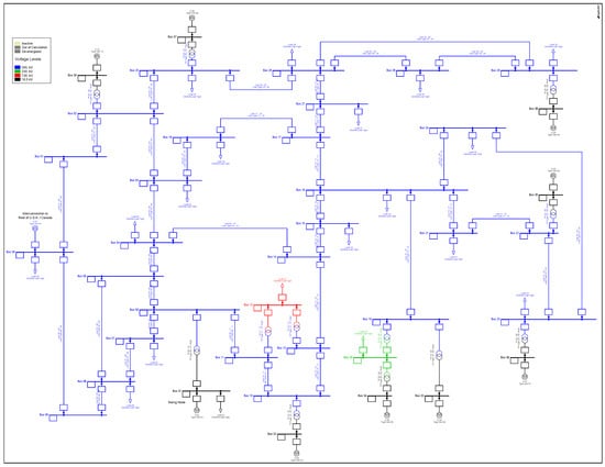
Figure 5.
Electrical configuration of the IEEE 39-bus system.
Table 7.
Standard power system 39 Bus-Bar.
Table 8.
Characterization of the transformers in the IEEE 39-bus system.
6. Numerical Validation
In this section it is presented all the computational validations of the proposed CBGA implemented in the DPL environment from the DigSILENT software to solve the optimal reactive power flow problem in power systems. These validations were carried out in a personal computer AMD Ryzen 5 3500U processor 2.10 GHz. RAM 8 Gb, with a Windows 10 operating system, single language, 64 bits.
6.1. IEEE 6-Bus System
Table 9 presents the results provided by the CBGA in the IEEE 6-bus system considering that in the scenarios A1 and A2 the maximum output voltage was limited to 1.1 pu, while for scenarions B1 and B2, this limit was increased to 1.15 pu. In the case of the slack bus, its voltage outputs were assigned in 1.05 pu for scenarios A1 and A2, and 1.10 pu for scenarios B1 and B2, respectively.
Table 9.
Numerical results for the CBGA implemented in DPL environment from DigSILENT applied to the IEEE 6-bus system.
Numerical results in Table 9 show that: (i) for all the simulation scenarios the power losses vary from to ; the improvement in the power losses reduction is mainly attributed to the fact that when compared scenarios A1 and A2 with B1 and B2, the voltage in the slack source is increased and the maximum voltage limits are also increased, which are directly related with the reduction of the current magnitudes through the lines and transformers, i.e., related directly with the reduction of the total power losses; (ii) regarding the reactive power injection in the capacitor banks, it is observed that these are closer to the 5 Mvar, which implies that these are assigned to their maximum limit. This situation occurs mainly due to the high inductive load profiles on the grid added with the inductive losses in lines and transformers; (iii) in the case of transformers, these are inclined to the maximum tap position, i.e., 11,100, where the voltage is incremented with respect to the nominal voltage output; which as mentioned below implies that the larger the voltage profiles the fewer power losses are achieved.
Table 10 presents the line chargeability at each simulation scenario. It is worth mentioning that the progressive increments in the voltage profiles for all nodes of the network, effectively, reduce the amount of current flow though the lines.
Table 10.
Line chargeability for the IEEE 6-bus system at each simulation scenario.
Note that there are some transmission lines that reduce their chargeability up to 10%; for example, the line 6-4 that passes from an initial condition of 55.80% to 44.40% in the simulation scenario B2; which is translated into an effective reduction of about 20% with respect to the initial operation scenario.
Figure 6 depicts the amount of power losses in kW for each one of the simulation scenarios and its comparison to the benchmark case. Notice that the simulation scenarios A2 and B2 are the cases where the voltage output at the slack node was set at 1.10 pu. In these scenarios is where the most important reductions in power losses are reached, with improvements of about respect to the benchmark case. In addition, for the simulation cases A1 and B1 where the voltage output at the slack node was set at 1.05 pu, the total reduction of power losses with respect to the benchmark case was about 22%.
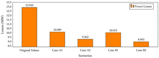
Figure 6.
Power Losses for all the simulation scenarios in the IEEE 6-bus system.
On the other hand, Figure 7 reports the behavior of the voltage profile at each simulation case including the benchmark case. Note that in general for all the simulation scenarios it is noted the improvement without violating the imposed maximum and minimum voltage regulation bounds.
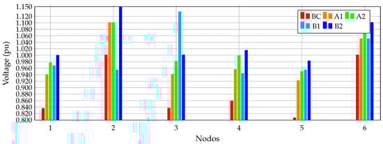
Figure 7.
Voltage profile performance in the IEEE 6-bus system for all the simulation scenarios.
Some of the buses of the network present important voltage improvements as the case of the bus 5, where the voltage magnitude is pu for the benchmark case, and for all the simulation scenarios, the improvement is reflected between 15% and 22%, with voltage magnitudes between 0.95 pu and 0.9 pu, respectively.
6.2. IEEE 14-Bus System
Table 11 reports the optimal reactive power outputs in shunt compensators, voltage outputs in generators, positions of the taps in transformers and the total power losses for each simulation scenario including the benchmark case. Observe that the amount of power losses vary from to from the scenario A1 to the scenario B2.
Table 11.
Numerical results for the CBGA implemented in DPL environment from DigSILENT applied to the IEEE 14-bus system.
When the capacitor banks are observed (being their nominal rates 20 Mvar for the compensator located at nodes PQBus06, and PQBus08, and 30 Mvar for the capacitor at bus PQB03), these are operated not necessarily in their upper bounds. For example, the scenario A2, after the implemetation of the CBGA in the DPL environment, the reactive power outputs in these capacitor banks were Mvar, Mvar, and Mvar, respectively.
Unlike the previous IEEE 6-bus system, where the tap of the transformers was set closer to their maximum values; in the IEEE 14-bus system, the behavior of these taps was different, being these variations mainly conditioned by the voltage outputs in the power generators, since not a particular tendency is evidenced on the transformers. Note that for the scenario A1, where the minimum and maximum bounds for all the tap positions were 9100 and 11,100, respectively, the mean values for the tap positions in this scenario were about 10415. Regarding the voltage outputs, it was observed that in the scenarios A1 and A2 where the maximum voltage bound was set to pu, the power generators provide voltages of pu and pu, respectively. This situation was repeated for the simulation scenarios B1 and B2 where the movement of the maximum voltage bound to pu is not an important effect of the voltage profiles, keeping these very similar to the simulation scenarios A1 and A2. The behavior of the voltage profiles in the different simulation scenarios is mainly attributable to the fact that the IEEE 14-bus system is a high-meshed network where the movement in one of the voltage output in a generator implies large variations in the total power losses.
In Table 12 is reported the chargeability percentage at each transmission line. For all the simulation scenarios this percentage is reduced with respect to the benchmark case. Note that there are some cases where transmission lines reduce their chargeability up to higher than . Notice that line 09-10 passes from % in the benchmark case to for the simulation scenario A1, and for the simulation scenario B2. In addition, the transmission line 12-13 presents a contrary behavior, where the benchmark case shows a chargearbiltiy of about and is increased to about for simulation cases A1, A2 and B1, and for the simulation scenario B2. However, this increment is associated with the load flow redistribution caused by the injection of reactive power with capacitor banks and active and reactive power outputs in generators. This does not increase significantly the amount of power losses, since most of the lines reduce their chargeability, which implies that in conjunction the total grid power losses is minimized.
Table 12.
Chargeability of Lines for the IEEE 14-bus system.
Figure 8 presents the amount of power losses in the IEEE 14-bus system in kW for all the simulation scenarios including the benchmark case. Note that the simulation cases A2 and B2 where the slack bus was set with an operative voltage of pu, the reduction of power losses are prominent with reductions of about with respect to the benchmark case. In the case of the simulation cases A1 and B1, where the voltage output in the slack node was fixed in pu, the average reduction of the power losses with respect to the benchmark case was about 21%. These results show the importance of the effect that has the voltage output in the reference bus, since this directly conditioned the expected power losses in the whole grid.
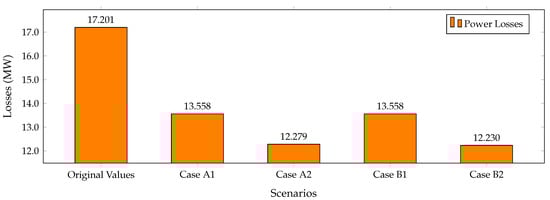
Figure 8.
Power Losses for all the simulation scenarios in the IEEE 14-bus system.
Figure 9 reports the voltage profile at each bus for all the simulation scenarios, where is evidenced that the optimal reactive power improves these when compared with the benchmark case without violating the lower and upper voltage bounds assigned at each simulation case.
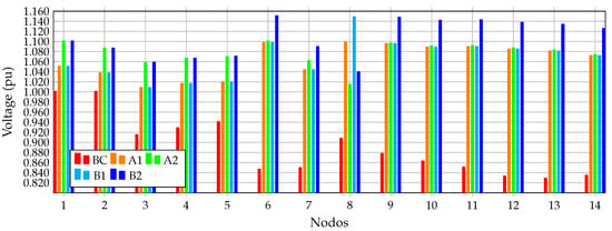
Figure 9.
Voltage profile performance in the IEEE 14-bus system for all the simulation scenarios.
Note that some of the buses show important improvements in their voltage magnitudes as the cases of the buses 12 and 13, which had magnitudes of pu and pu in the benchmark case; however, for all the four simulation scenarios the improvements were about , being both buses with a voltage value of pu in the scenario A1, with pu; and in scenario B2 the voltage in buses 12 and 13 were pu and pu, respectively, when pu. A general conclusion after implementing the CBGA in the DPL environment for the IEEE 14-bus system is that all the voltage profiles present improvements higher than for all the simulation cases when compared with the benchmark case. This is a result from increasing the voltage output in the slack bus, the injection of reactive power through the capacitor banks and the modification of the tap position in all the transformers.
6.3. 39-Bus System
Table 13 reports the solutions reached by the proposed CBGA in the DPL environment from DigSILENT for the IEEE 39-bus system. Note that for all the simulation cases were obtained reductions in the total grid power losses from to .
Table 13.
Numerical results for the CBGA implemented in DPL environment from DigSILENT applied to the IEEE 39-bus system.
An important fact is that this system does not include in their topology reactive power compensators; however, due to the presence of 12 transformers and 9 power sources, with the proposed CBGA is possible to reach an optimal combination of the tap positions and voltage outputs that allows to achieve general power losses reduction higher than when compared to the benchmark case.
Regarding the tap positions in the transformers, there is no evidence of a general tendency towards the upper or lower bounds, and these are distributed in all the operative range. This situation is mainly justified on the high meshed connection of this system where the movement of one voltage magnitude in a particular node produces important effects on the grid. In addition, when the voltage output in the slack bus was set to pu and pu in the scenarios A1 and A2 with a maximum voltage regulation limit of pu, it is possible to observe that all the voltage profiles in the whole grid are between 1.02 pu and 1.098 pu, respectively.
Table 14 presents the percentage of chargeability of each one of the transmission lines in all the simulation cases for the IEEE 39-bus system. In general, all the lines present a reduction larger than of their chargeability when compared with the benchmark case. Notice the case of the line 03-04 that passes from of loadability in the benchmark case to for the scenario A1 and for the scenario A2, respectively. In addition, observe that the line 14-15 presents an increment in its loadability that passes from in the benchmark case to the in the scenario A2. This behavior is expected in power systems since the redistribution of the power flow through the lines implies that some of the lines with low loadability increases their power flow; however, these increments do not affect the objective function and in general, this reaches its optimum value.
Table 14.
Chargeability of the lines for the IEEE 39-bus system.
On the other hand, in Figure 10 it is reported the amount of power losses in kW for the IEEE 39-bus system in the benchmark case and the proposed simulation scenarios. Note that scenarios B1 and B2 present higher reductions with respect to the benchmark case which are about 37%. These results are justified in the fact that for these simulation cases all the maximum voltage limit is pu, while for scenarios A1 and A2 this limit is pu. This implies that without the presence of capacitor banks, the unique form to reduce the total power losses on the whole grid is via increasing the voltage outputs in all the generators.
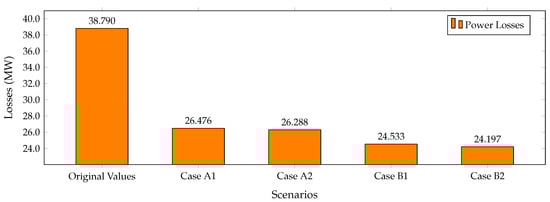
Figure 10.
Power Losses with genetic algorithm in IEEE-39 bus-bar.
Finally, Figure 11 reports the voltage profile performance for all the nodes in all the simulation scenarios including the benchmark case. Note that all the voltage profiles remain within their bounds for each scenario; which implies that the proposed CBGA ensures the feasibility of the solution with high-quality regarding the objective function value.
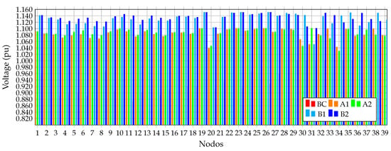
Figure 11.
Voltage profile performance in the IEEE 39-bus system for all the simulation scenarios.
In the IEEE 39-bus system, some of the buses present important improvements in their voltage profiles. See the nodes 10 and 12, which in the benchmark case have voltage values of pu and pu; nevertheless, for all the simulation scenarios these were improved in more than reaching values of 1.09 pu and 1.07 pu in the scenario A1 and, 1.13 pu and 1.11 pu for the scenario B1, respectively. It is worth mentioning that in general the improvement of the voltage profiles of the nodes was about 15% in the four studied scenarios of simulation.
6.4. Processing Times
To demonstrate the effectiveness and robustness of the proposed CBGA implemented in the DPL environment from DigSILENT to resolve the optimal reactive power flow problem in transmission networks, we report in Table 15 the average processing times for all the IEEE bus systems.
Table 15.
Average processing times for all the IEEE bus systems in the four studied scenarios.
Note that as is expected, when the number of nodes increases, the total processing times are increased due to computational effort in the power flow evaluation considering that the number of the decision variables is directly related to the size of the power system under study. Note that the average time for all the simulation cases is s for the IEEE 6-bus system, s for the IEEE 14-bus system, and s for the IEEE 39-bus system, respectively. Note that for calculating these processing times, the proposed CBGA was evaluated 100 times per simulation scenario; in addition, the proposed CBGA was set with a random population of 1000 individuals, which is ordered to obtain the best 20 individuals that define the initial population, and 10,000 iterations are considered during the exploration and exploitation of the solution space. It is worth mentioning that all the descending individuals are crossed and mutated.
7. Conclusions
The optimal reactive power flow problem in transmission systems was addressed in this research from the point of view of the combinatorial optimization by implementing a CBGA in DPL environment from DigSILENT software. The main advantage of using the DPL is that all the functionalities of the DigSILENT software for system modeling and power calculations can be easily used with its own programming objects. The computational validations of the proposed solution methodology was carried-out in three IEEE power systems composed of 6, 14 and 39 buses, considering as optimization variables the voltage outputs in generators, tap position in transformers and reactive power injection in capacitor Banks. Four simulation scenarios were considered with the modification on the voltage in the slack bus and the maximum voltage regulation bounds, with the purpose of validating the effectiveness of the proposed CBGA in the DPL environment.
Numerical results in all the three IEEE test systems demonstrated that the percentage of reduction for the power losses was within to with respect to benchmark case. In the case of the IEEE 6-bus system the minimum and maximum reductions were 21.85% and 30.56% for the scenarios A1 and B2; the IEEE 14-bus system reported 21.17% and 28.90% for the scenarios B1 and B2 (21.18% for the scenario A1) and in the IEEE 39-bus systems these values were and for scenarios A1 and B2, respectively. It was noted that the voltage magnitude in the slack node strongly conditioned the percentage of power losses reduction, since for scenarios A1 and B1 where the slack was fixed in 1.05 pu, the reduction of power losses were considerably less than the scenarios A2 and B2 where were set in 1.10 pu, respectively.
The loadability of the transmission lines was in general reduced for all the test systems with average values between for the IEEE 6-bus and IEEE 14-bus systems, and , with two particular cases in the IEEE 14- and 39-bus systems, where the chargeability in some lines with low loadability <5% increase their values up to at most. This behavior is explained due to the power flow redistribution of the variations in the power injections in generators, tap positions in transformers and reactive power injections in capacitor banks.
As future works it will be possible to develop the following researches: (i) to implement recent developed discrete-continuous algorithms such as the vortex search algorithm and the sine cosine algorithm to solve the problem addressed in this study; and (ii) to implement in the DPL environment from DigSILENT a solution for the problem of the optimal reactive power compensation using STATCOMs and fixed-step capacitor banks.
Author Contributions
Conceptualization, D.L.B.-R.; O.D.M. and A.A.-L.; Methodology, D.L.B.-R.; O.D.M. and A.A.-L.; Investigation, D.L.B.-R.; O.D.M. and A.A.-L.; and Writing—review and editing, D.L.B.-R.; O.D.M. and A.A.-L. All authors have read and agreed to the published version of the manuscript.
Funding
This work was supported in part by the Centro de Investigación y Desarrollo Científico de la Universidad Distrital Francisco José de Caldas under grant 1643-12-2020 associated with the project: “Desarrollo de una metodología de optimización para la gestión óptima de recursos energéticos distribuidos en redes de distribución de energía eléctrica”.
Institutional Review Board Statement
Not applicable.
Informed Consent Statement
Not applicable.
Data Availability Statement
Data is contained within the article.
Acknowledgments
This work has been derived from the undergraduate project: “Flujo de potencia óptimo reactivo empleando un algoritmo genético discreto-continuo implementado en el lenguaje de programación de DigSILENT” presented by the student David Lionel Bernal Romero to the Electrical Engineering Program of the Engineering Faculty at Universidad Distrital Francisco José de Caldas as a partial requirement for the Bachelor in Electrical Engineering.
Conflicts of Interest
The authors declare no conflict of interest.
Nomenclature
| Set that contains all the capacitor banks installed. | |
| Set that contains all the generators of the network. | |
| Set that contains all the reactors installed. | |
| Set that contains all the nodes of the network. | |
| Set that contains all the transformers on the network. | |
| Angle of the admittance that relates nodes k and m (rad). | |
| Angle of the voltage at node k (rad). | |
| Angle of the voltage at node m (rad). | |
| a | Index associated with the transformers. |
| Tap position for the capacitor bank. | |
| Upper bound for the tap position in the capacitor bank. | |
| lower bound for the tap position in the capacitor bank. | |
| j | Index associated with the capacitor banks. |
| Sub-indices associated with nodes. | |
| l | Index associated with the reactors. |
| Active power consumption at node k (W). | |
| Active power generation at node k (W). | |
| Objective function value associated with the grid power losses (W). | |
| Reactive power injection through the capacitor bank connected at node k (VAr). | |
| Reactive power consumption at node k (VAr). | |
| Reactive power generation at node k (VAr). | |
| Reactive power absorption through the reactor connected at node k (VAr). | |
| Tap position for the reactor. | |
| Upper bound for the tap position in the reactor. | |
| lower bound for the tap position in the reactor. | |
| Tap position in the transformer. | |
| Maximum bound for the tap position in the transformer. | |
| Minimum bound for the tap position in the transformer. | |
| Maximum voltage bound for the output voltage in the generator i (V). | |
| Minimum voltage bound for the output voltage in the generator i (V). | |
| Magnitude of the output voltage in the generator i (V). | |
| Magnitude of the voltage at node k (V). | |
| Maximum voltage bound for the voltage at node k (V). | |
| Minimum voltage bound for the voltage at node k (V). | |
| Magnitude of the voltage at node m (V). | |
| Magnitude of the admittance that relates nodes k and m (rad). |
References
- Murty, P. Power flow studies. In Power Systems Analysis; Elsevier: Amsterdam, The Netherlands, 2017; pp. 205–276. [Google Scholar] [CrossRef]
- Alamri, B.; Hossain, M.A.; Asghar, M.S.J. Electric Power Network Interconnection: A Review on Current Status, Future Prospects and Research Direction. Electronics 2021, 10, 2179. [Google Scholar] [CrossRef]
- Lam, C.S.; Wong, M.C.; Han, Y.D. Voltage Swell and Overvoltage Compensation With Unidirectional Power Flow Controlled Dynamic Voltage Restorer. IEEE Trans. Power Deliv. 2008, 23, 2513–2521. [Google Scholar] [CrossRef]
- Montoya, O.D.; Fuentes, J.E.; Moya, F.D.; Barrios, J.Á.; Chamorro, H.R. Reduction of Annual Operational Costs in Power Systems through the Optimal Siting and Sizing of STATCOMs. Appl. Sci. 2021, 11, 4634. [Google Scholar] [CrossRef]
- Villa-Acevedo, W.; López-Lezama, J.; Valencia-Velásquez, J. A Novel Constraint Handling Approach for the Optimal Reactive Power Dispatch Problem. Energies 2018, 11, 2352. [Google Scholar] [CrossRef]
- Londoño, D.C.; Villa-Acevedo, W.M.; López-Lezama, J.M. Assessment of metaheuristic techniques applied to the optimal reactive power dispatch. In Communications in Computer and Information Science; Springer International Publishing: New York, NY, USA, 2019; pp. 250–262. [Google Scholar] [CrossRef]
- Rojas, D.G.; Lezama, J.L.; Villa, W. Metaheuristic Techniques Applied to the Optimal Reactive Power Dispatch: A Review. IEEE Lat. Am. Trans. 2016, 14, 2253–2263. [Google Scholar] [CrossRef]
- Ara, A.L.; Kazemi, A.; Gahramani, S.; Behshad, M. Optimal reactive power flow using multi-objective mathematical programming. Sci. Iran. 2012, 19, 1829–1836. [Google Scholar] [CrossRef]
- Duong, T.L.; Duong, M.Q.; Phan, V.D.; Nguyen, T.T. Optimal Reactive Power Flow for Large-Scale Power Systems Using an Effective Metaheuristic Algorithm. J. Electr. Comput. Eng. 2020, 2020, 6382507. [Google Scholar] [CrossRef]
- Aghbolaghi, A.J.; Tabatabaei, N.M.; Boushehri, N.S.; Parast, F.H. Reactive power optimization in AC power systems. In Power Systems; Springer International Publishing: New York, NY, USA, 2017; pp. 345–409. [Google Scholar] [CrossRef]
- Naderi, E.; Narimani, H.; Fathi, M.; Narimani, M.R. A novel fuzzy adaptive configuration of particle swarm optimization to solve large-scale optimal reactive power dispatch. Appl. Soft Comput. 2017, 53, 441–456. [Google Scholar] [CrossRef]
- Saddique, M.S.; Bhatti, A.R.; Haroon, S.S.; Sattar, M.K.; Amin, S.; Sajjad, I.A.; ul Haq, S.S.; Awan, A.B.; Rasheed, N. Solution to optimal reactive power dispatch in transmission system using meta-heuristic techniques—Status and technological review. Electr. Power Syst. Res. 2020, 178, 106031. [Google Scholar] [CrossRef]
- Zhao, J.; Zhang, Z.; Yao, J.; Yang, S.; Wang, K. A distributed optimal reactive power flow for global transmission and distribution network. Int. J. Electr. Power Energy Syst. 2019, 104, 524–536. [Google Scholar] [CrossRef]
- Yoshida, H.; Kawata, K.; Fukuyama, Y.; Takayama, S.; Nakanishi, Y. A particle swarm optimization for reactive power and voltage control considering voltage security assessment. IEEE Trans. Power Syst. 2000, 15, 1232–1239. [Google Scholar] [CrossRef]
- Esmin, A.; Lambert-Torres, G.; de Souza, A.Z. A hybrid particle swarm optimization applied to loss power minimization. IEEE Trans. Power Syst. 2005, 20, 859–866. [Google Scholar] [CrossRef]
- Mahadevan, K.; Kannan, P. Comprehensive learning particle swarm optimization for reactive power dispatch. Appl. Soft Comput. 2010, 10, 641–652. [Google Scholar] [CrossRef]
- Singh, R.P.; Mukherjee, V.; Ghoshal, S. Optimal reactive power dispatch by particle swarm optimization with an aging leader and challengers. Appl. Soft Comput. 2015, 29, 298–309. [Google Scholar] [CrossRef]
- Gutiérrez, D.; Villa, W.M.; López-Lezama, J.M. Flujo Óptimo Reactivo mediante Optimización por Enjambre de Partículas. Inf. Tecnológica 2017, 28, 215–224. [Google Scholar] [CrossRef][Green Version]
- Duman, S.; Sonmez, Y.; Guvencc, U.; Yorukeren, N. Optimal reactive power dispatch using a gravitational search algorithm. IET Gener. Transm. Distrib. 2012, 6, 563. [Google Scholar] [CrossRef]
- Shaw, B.; Mukherjee, V.; Ghoshal, S. Solution of reactive power dispatch of power systems by an opposition-based gravitational search algorithm. Int. J. Electr. Power Energy Syst. 2014, 55, 29–40. [Google Scholar] [CrossRef]
- Mei, R.N.S.; Sulaiman, M.H.; Mustaffa, Z.; Daniyal, H. Optimal reactive power dispatch solution by loss minimization using moth-flame optimization technique. Appl. Soft Comput. 2017, 59, 210–222. [Google Scholar] [CrossRef]
- Ela, A.A.E.; Abido, M.; Spea, S. Differential evolution algorithm for optimal reactive power dispatch. Electr. Power Syst. Res. 2011, 81, 458–464. [Google Scholar] [CrossRef]
- Bhongade, S.; Tomar, A.; Goigowal, S.R. Minimization of optimal reactive power dispatch problem using BAT algorithm. In Proceedings of the 2020 IEEE First International Conference on Smart Technologies for Power, Energy and Control (STPEC), Online. 25–26 September 2020. [Google Scholar] [CrossRef]
- Bakirtzis, A.; Biskas, P.; Zoumas, C.; Petridis, V. Optimal power flow by enhanced genetic algorithm. IEEE Trans. Power Syst. 2002, 17, 229–236. [Google Scholar] [CrossRef]
- Abido, M.A. Optimal Power Flow Using Tabu Search Algorithm. Electr. Power Compon. Syst. 2002, 30, 469–483. [Google Scholar] [CrossRef]
- Lenin, K. Reduction of active power loss by improved tabu search algorithm. Int. J. Res.—GRANTHAALAYAH 2018, 6, 1–9. [Google Scholar] [CrossRef]
- ElSayed, S.K.; Elattar, E.E. Slime Mold Algorithm for Optimal Reactive Power Dispatch Combining with Renewable Energy Sources. Sustainability 2021, 13, 5831. [Google Scholar] [CrossRef]
- Ganesh, S.; Perilla, A.; Torres, J.R.; Palensky, P.; van der Meijden, M. Validation of EMT Digital Twin Models for Dynamic Voltage Performance Assessment of 66 kV Offshore Transmission Network. Appl. Sci. 2020, 11, 244. [Google Scholar] [CrossRef]
- Tabatabaei, N.M.; Aghbolaghi, A.J.; Boushehri, N.S.; Parast, F.H. Reactive power optimization using MATLAB and DIgSILENT. In Power Systems; Springer International Publishing: New York, NY, USA, 2017; pp. 411–474. [Google Scholar] [CrossRef]
- Castiblanco-Pérez, C.M.; Toro-Rodríguez, D.E.; Montoya, O.D.; Giral-Ramírez, D.A. Optimal Placement and Sizing of D-STATCOM in Radial and Meshed Distribution Networks Using a Discrete-Continuous Version of the Genetic Algorithm. Electronics 2021, 10, 1452. [Google Scholar] [CrossRef]
- Villena-Ruiz, R.; Honrubia-Escribano, A.; Fortmann, J.; Gómez-Lázaro, E. Field validation of a standard Type 3 wind turbine model implemented in DIgSILENT-PowerFactory following IEC 61400-27-1 guidelines. Int. J. Electr. Power Energy Syst. 2020, 116, 105553. [Google Scholar] [CrossRef]
- Bifaretti, S.; Bonaiuto, V.; Pipolo, S.; Terlizzi, C.; Zanchetta, P.; Gallinelli, F.; Alessandroni, S. Power Flow Management by Active Nodes: A Case Study in Real Operating Conditions. Energies 2021, 14, 4519. [Google Scholar] [CrossRef]
- Barboza, L.V.; Ziirn, H.H.; Salgado, R. Load Tap Change Transformers: A Modeling Reminder. IEEE Power Eng. Rev. 2001, 21, 51–52. [Google Scholar] [CrossRef]
- Londoño-Tamayo, D.; Villa-Acevedo, J.L.L.W. Mean-Variance Mapping Optimization Algorithm Applied to the Optimal Reactive Power Dispatch. INGECUC 2021, 17, 239–255. [Google Scholar] [CrossRef]
- Sharif, S.; Taylor, J. MINLP formulation of optimal reactive power flow. In Proceedings of the 1997 American Control Conference (Cat. No.97CH36041), Albuquerque, NM, USA, 6 June 1997. [Google Scholar] [CrossRef]
- Morán-Burgos, J.A.; Sierra-Aguilar, J.E.; Villa-Acevedo, W.M.; López-Lezama, J.M. A Multi-Period Optimal Reactive Power Dispatch Approach Considering Multiple Operative Goals. Appl. Sci. 2021, 11, 8535. [Google Scholar] [CrossRef]
- DIgSILENT GmbH. DIgSILENT PowerFactory Version 15, User Manual; DIgSILENT GmbH: Gomaringen, Germany, 2014. [Google Scholar]
- Gaitán, L.F.; Gómez, J.D.; Rivas-Trujillo, E. Quasi-Dynamic Analysis of a Local Distribution System with Distributed Generation. Study Case: The IEEE 13 Node System. TecnoLógicas 2019, 22, 195–212. [Google Scholar] [CrossRef]
- Cortés-Caicedo, B.; Avellaneda-Gómez, L.S.; Montoya, O.D.; Alvarado-Barrios, L.; Chamorro, H.R. Application of the Vortex Search Algorithm to the Phase-Balancing Problem in Distribution Systems. Energies 2021, 14, 1282. [Google Scholar] [CrossRef]
- Gonzalez-Longatt, F.M.; Rueda, J.L. (Eds.) PowerFactory Applications for Power System Analysis; Springer International Publishing: New York, NY, USA, 2014. [Google Scholar] [CrossRef]
Publisher’s Note: MDPI stays neutral with regard to jurisdictional claims in published maps and institutional affiliations. |
© 2021 by the authors. Licensee MDPI, Basel, Switzerland. This article is an open access article distributed under the terms and conditions of the Creative Commons Attribution (CC BY) license (https://creativecommons.org/licenses/by/4.0/).