
Kidney Cancer Diagnosis and Surgery Selection by Machine Learning from CT Scans Combined with Clinical Metadata

 ,
,  ,
, 
Simple Summary
Abstract
1. Introduction
- Computed tomography (CT) images and clinical metadata from the KiTS21 dataset were used to differentiate four major classes of renal cancer: clear cell (ccRCC), chromophobe (chRCC), papillary (pRCC) renal cell carcinoma, and oncocytoma (ONC);
- Tumor subclass predictions were integrated with clinical metadata to determine the optimal surgical approach in malignant cases (radical versus partial nephrectomy);
- To the best of our knowledge, this is the first study to determine kidney tumor subclass using a combination of CT images and corresponding clinical features;
- This pioneering study paves the way for future refinement of tools that can guide surgical interventions in kidney cancer by applying machine-learning algorithms trained on relevant clinical data.
2. Related Work
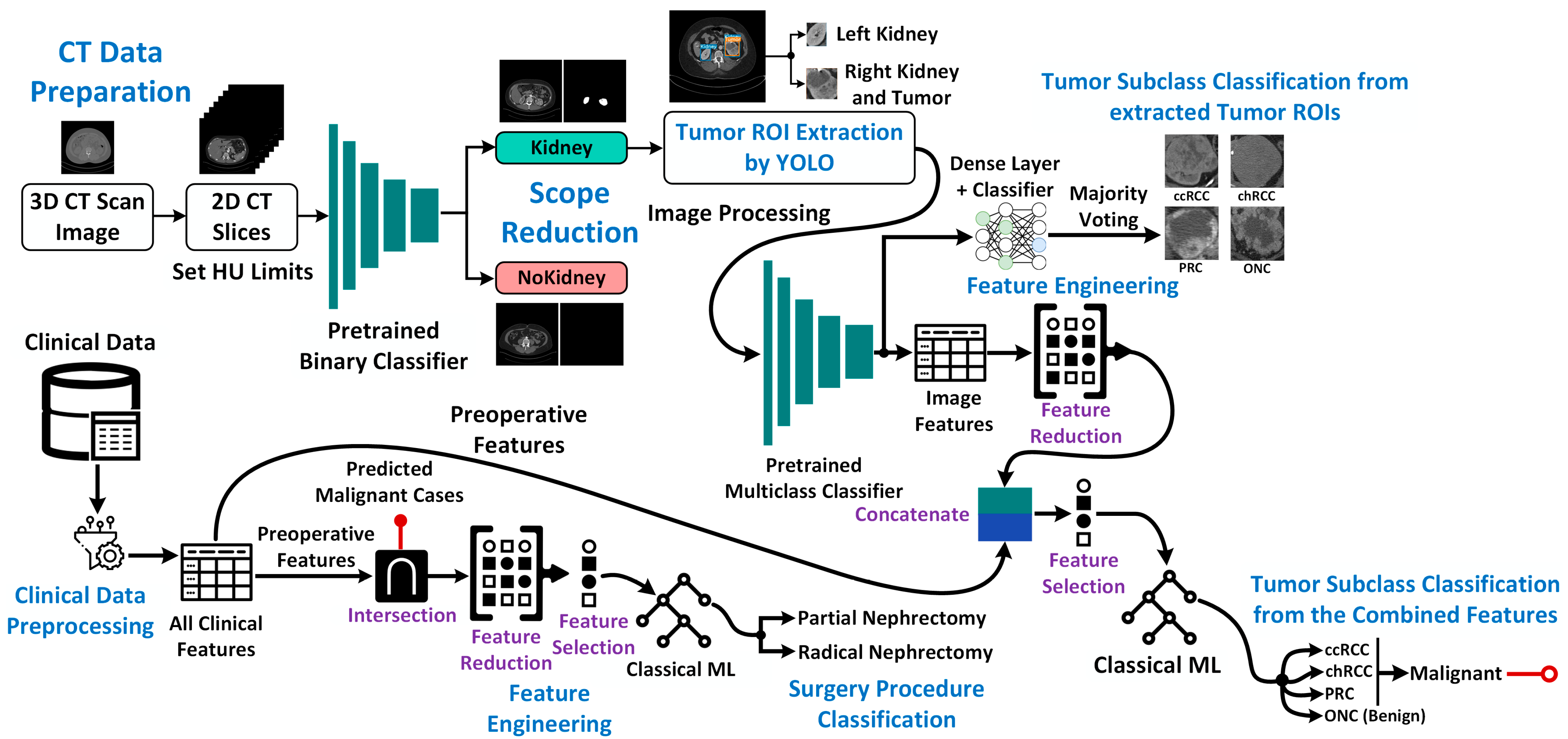
3. Methodology
3.1. Dataset Description
3.2. Preprocessing of Computed Tomography (CT) Images
3.3. Scope Reduction through Kidney Instance Classification
DenseAUXNet201 Architecture
3.4. Region of Interest (ROI) Extraction from 2D-CT Slices
3.4.1. Bounding Box Label Generation from Segmentation Masks
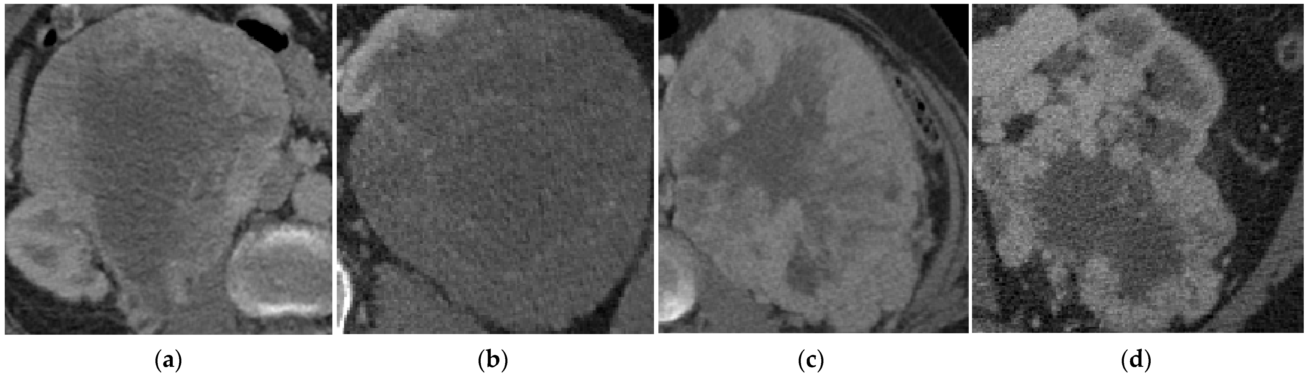
3.5. Kidney Tumor Subtype Classification from Extracted CT ROIs
3.6. Tumor Subtype and Surgery Procedure Classification from Clinical or Combined Data
3.6.1. Clinical Data Pre-Processing
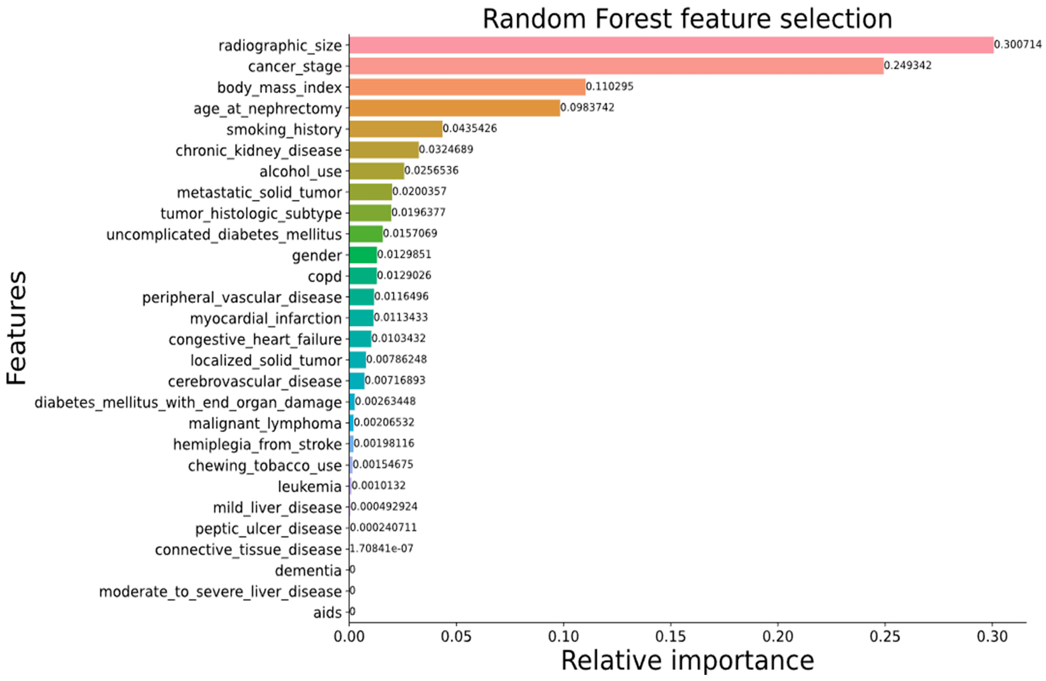
3.6.2. Feature Engineering
3.6.3. Classical Machine-Learning Algorithms
3.7. Quantitative Evaluation Metrics
3.7.1. Classification
3.7.2. Object Detection
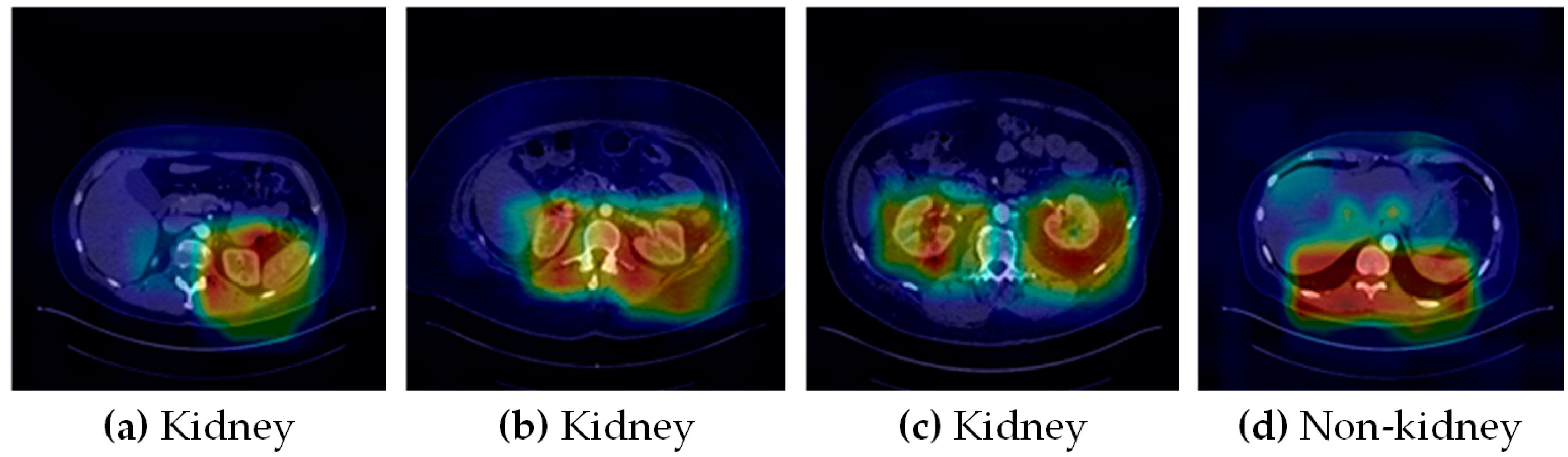
3.8. Qualitative Evaluation
4. Experimental Results
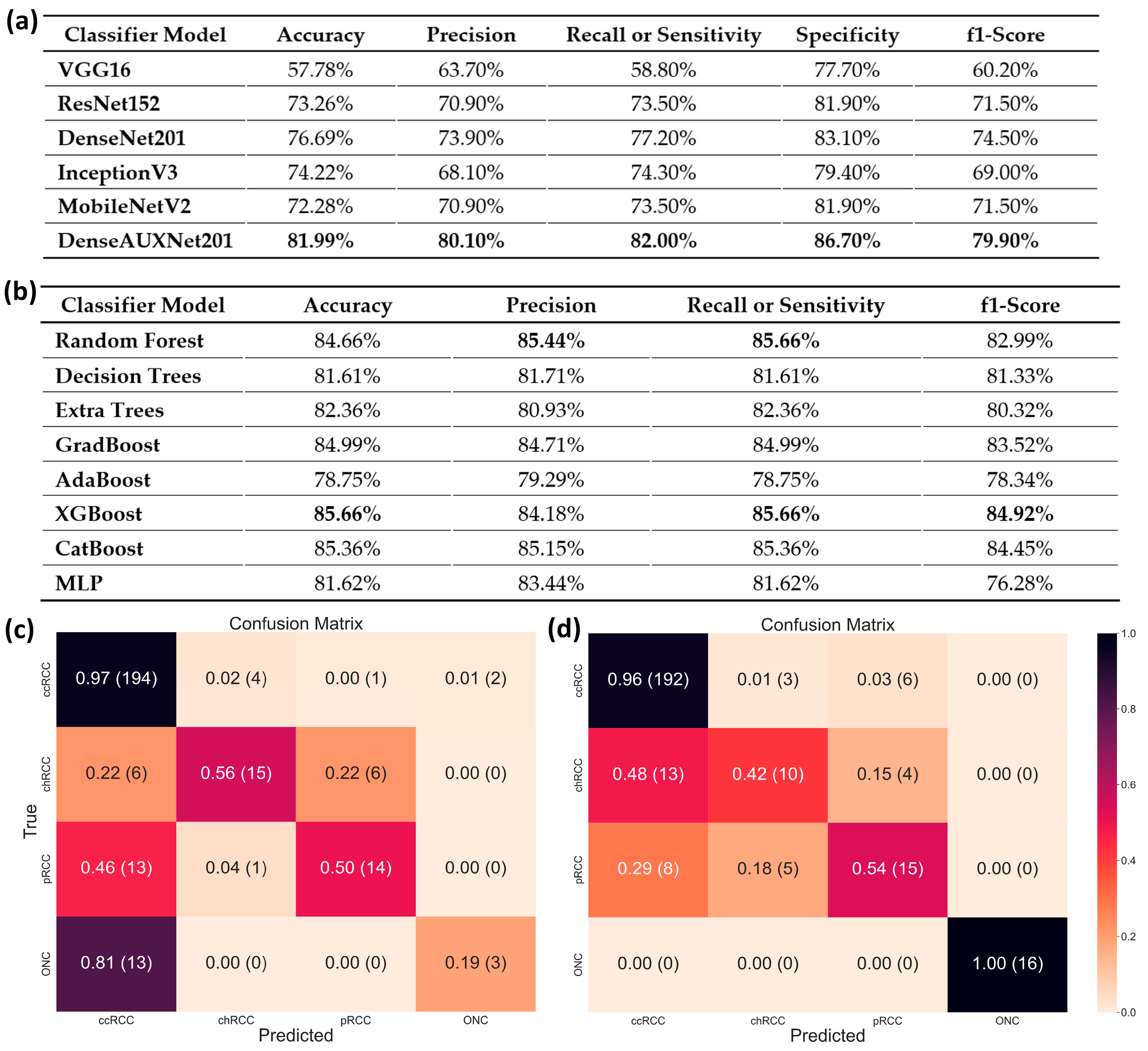
4.1. Kidney Tumor Classification
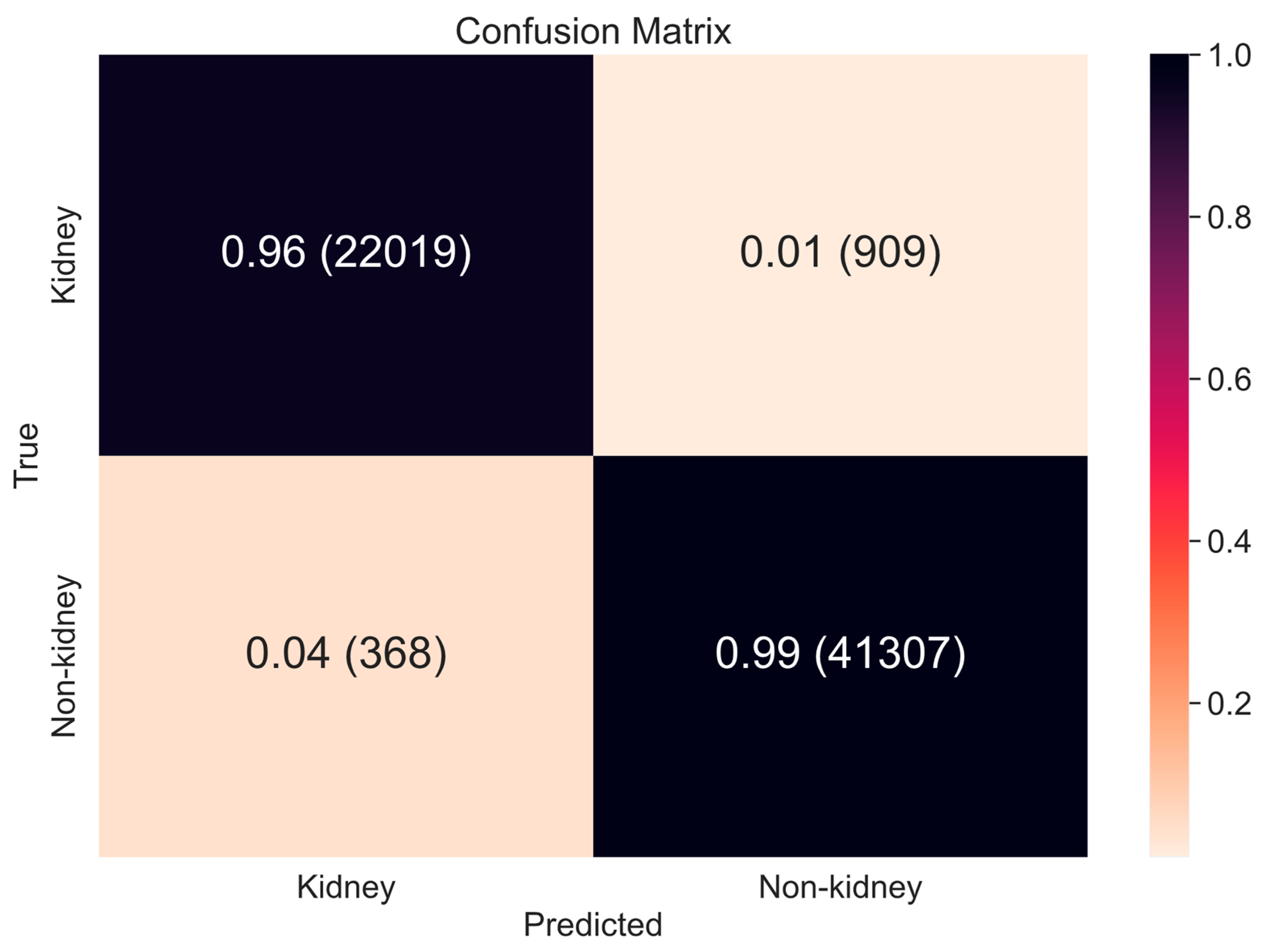
4.1.1. Scope Reduction through Binary Classification
4.1.2. Region of Interest (ROI) Extraction from 2D-CT Slices using YOLO
4.1.3. Kidney Cancer Subtype Classification from Tumor ROIs and Clinical Metadata
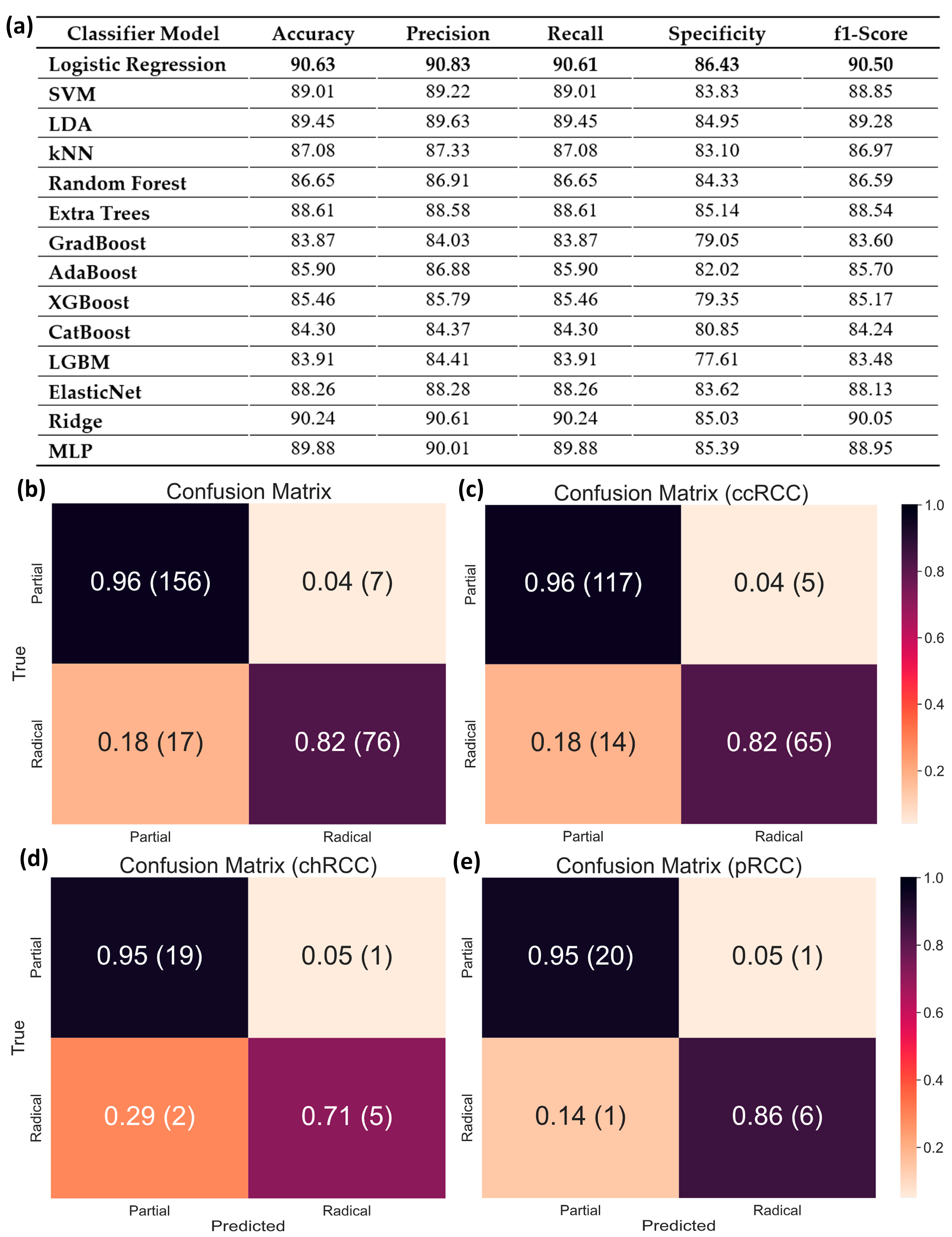
4.2. Surgical Procedure Determination from Clinical Data for Malignant Tumors
5. Conclusions
Supplementary Materials
Author Contributions
Funding
Institutional Review Board Statement
Informed Consent Statement
Data Availability Statement
Conflicts of Interest
References
- Mayo Clinic. Chronic Kidney Disease. 3 September 2021. Available online: https://www.mayoclinic.org/diseases-conditions/chronic-kidney-disease/symptoms-causes/syc-20354521 (accessed on 25 March 2023).
- Kovesdy, C.P. Epidemiology of chronic kidney disease: An update 2022. Kidney Int. Suppl. 2022, 12, 7–11. [Google Scholar] [CrossRef] [PubMed]
- WCRF International. Kidney Cancer Statistics: World Cancer Research Fund International. 14 April 2022. Available online: https://www.wcrf.org/cancer-trends/kidney-cancer-statistics (accessed on 26 March 2023).
- Ito, C.; Nagata, D. Profound connection between chronic kidney disease and both colorectal cancer and renal cell carcinoma. J. Kidney 2016, 2, 1000118. [Google Scholar]
- Hu, M.; Wang, Q.; Liu, B.; Ma, Q.; Zhang, T.; Huang, T.; Lv, Z.; Wang, R. Chronic kidney disease and cancer: Inter-relationships and Mechanisms. Front. Cell Dev. Biol. 2022, 10, 1073. [Google Scholar] [CrossRef] [PubMed]
- Webster, A.C.; Nagler, E.V.; Morton, R.L.; Masson, P. Chronic kidney disease. Lancet 2017, 389, 1238–1252. [Google Scholar] [CrossRef] [PubMed]
- Saly, D.L.; Eswarappa, M.S.; Street, S.E.; Deshpande, P. Renal cell cancer and chronic kidney disease. Adv. Chronic Kidney Dis. 2021, 28, 460–468. [Google Scholar] [CrossRef]
- Lees, J.S.; Elyan, B.M.; Herrmann, S.M.; Lang, N.N.; Jones, R.J.; Mark, P.B. The “other” big complication: How chronic kidney disease impacts on cancer risks and outcomes. Nephrol. Dial. Transplant. 2022, 38, 1071–1079. [Google Scholar] [CrossRef]
- Hussain, M.A.; Hamarneh, G.; Garbi, R. Cascaded Regression Neural Nets for Kidney Localization and Segmentation-free Volume Estimation. IEEE Trans. Med. Imaging 2021, 40, 1555–1567. [Google Scholar] [CrossRef]
- NHS Choices. Available online: https://www.nhs.uk/conditions/autosomal-dominant-polycystic-kidney-disease-adpkd/ (accessed on 25 March 2023).
- Cleveland Clinic. Renal Artery Stenosis: Symptoms, Causes, and Treatment. Available online: https://my.clevelandclinic.org/health/diseases/17422-renal-artery-disease (accessed on 25 March 2023).
- Pennmedicine.org. End-Stage Kidney Disease. Available online: https://www.pennmedicine.org/for-patients-and-visitors/patient-information/conditions-treated-a-to-z/end-stage-kidney-disease (accessed on 25 March 2023).
- American Kidney Fund. Blood Test: EGFR (Estimated Glomerular Filtration Rate). 24 January 2023. Available online: https://www.kidneyfund.org/all-about-kidneys/tests/blood-test-egfr (accessed on 25 March 2023).
- National Kidney Foundation. ACR. 11 May 2017. Available online: https://www.kidney.org/kidneydisease/siemens_hcp_acr (accessed on 25 March 2023).
- National Institute of Biomedical Imaging and Bioengineering. X-rays. Available online: https://www.nibib.nih.gov/science-education/science-topics/x-rays (accessed on 25 March 2023).
- Cleveland Clinic. Kidney Ultrasound: Procedure Information, Preparation, and Results. Available online: https://my.clevelandclinic.org/health/diagnostics/15764-kidney-ultrasound (accessed on 25 March 2023).
- Johns Hopkins Medicine. Computed Tomography (CT or CAT) Scan of the Kidney. 8 August 2021. Available online: https://www.hopkinsmedicine.org/health/treatment-tests-and-therapies/ct-scan-of-the-kidney (accessed on 25 March 2023).
- Tomboc, K.; Ezra. MRI of the Kidney: Your Guide for Preventative Screening. 29 July 2022. Available online: https://ezra.com/kidney-mri/ (accessed on 26 March 2023).
- Krishnan, N.; Perazella, M.A. The role of PET scanning in the evaluation of patients with kidney disease. Adv. Chronic Kidney Dis. 2017, 24, 154–161. [Google Scholar] [CrossRef]
- Tests for Kidney Cancer. Kidney Cancer Diagnosis. Available online: https://www.cancer.org/cancer/kidney-cancer/detection-diagnosis-staging/how-diagnosed.html (accessed on 25 March 2023).
- Shubham, S.; Jain, N.; Gupta, V.; Mohan, S.; Ariffin, M.M.; Ahmadian, A. Identify glomeruli in human kidney tissue images using a deep learning approach. Soft Comput. 2021, 27, 2705–2716. [Google Scholar] [CrossRef]
- Elton, D.C.; Turkbey, E.B.; Pickhardt, P.J.; Summers, R.M. A deep learning system for Automated Kidney Stone Detection and volumetric segmentation on noncontrast CT scans. Med. Phys. 2022, 49, 2545–2554. [Google Scholar] [CrossRef]
- Abdelrahman, A.; Viriri, S. Kidney tumor semantic segmentation using Deep Learning: A Survey of state-of-the-art. J. Imaging 2022, 8, 55. [Google Scholar] [CrossRef]
- Smail, L.C.; Dhindsa, K.; Braga, L.H.; Becker, S.; Sonnadara, R.R. Using deep learning algorithms to grade hydronephrosis severity: Toward a clinical adjunct. Front. Pediatr. 2020, 8, 1. [Google Scholar] [CrossRef]
- Uhm, K.-H.; Jung, S.-W.; Choi, M.H.; Shin, H.-K.; Yoo, J.-I.; Oh, S.W.; Kim, J.Y.; Kim, H.G.; Lee, Y.J.; Youn, S.Y.; et al. Deep learning for end-to-end kidney cancer diagnosis on multi-phase abdominal computed tomography. NPJ Precis. Oncol. 2021, 5, 54. [Google Scholar] [CrossRef]
- Mo, X.; Chen, W.; Chen, S.; Chen, Z.; Guo, Y.; Chen, Y.; Wu, X.; Zhang, L.; Chen, Q.; Jin, Z.; et al. MRI texture-based machine learning models for the evaluation of renal function on different segmentations: A proof-of-concept study. Insights Imaging 2023, 14, 28. [Google Scholar] [CrossRef] [PubMed]
- Alnazer, I.; Bourdon, P.; Urruty, T.; Falou, O.; Khalil, M.; Shahin, A.; Fernandez-Maloigne, C. Recent advances in medical image processing for the evaluation of chronic kidney disease. Med. Image Anal. 2021, 69, 101960. [Google Scholar] [CrossRef]
- Yao, L.; Zhang, H.; Zhang, M.; Chen, X.; Zhang, J.; Huang, J.; Zhang, L. Application of artificial intelligence in renal disease. Clin. eHealth 2021, 4, 54–61. [Google Scholar] [CrossRef]
- Rini, B.I.; Campbell, S.C.; Escudier, B. Renal cell carcinoma. Lancet 2009, 373, 1119–1132. [Google Scholar] [CrossRef] [PubMed]
- Hsieh, J.J.; Purdue, M.P.; Signoretti, S.; Swanton, C.; Albiges, L.; Schmidinger, M.; Heng, D.Y.; Larkin, J.; Ficarra, V. Renal cell carcinoma. Nat. Rev. Dis. Prim. 2017, 3, 17009. [Google Scholar] [CrossRef]
- Tanaka, T.; Huang, Y.; Marukawa, Y.; Tsuboi, Y.; Masaoka, Y.; Kojima, K.; Iguchi, T.; Hiraki, T.; Gobara, H.; Yanai, H.; et al. Differentiation of small renal masses on multiphase contrast-enhanced CT by deep learning. Am. J. Roentgenol. 2020, 214, 605–612. [Google Scholar] [CrossRef] [PubMed]
- Schneider, R.; Franciscan Health. Open, Laparoscopic and Robotic Surgery: What to Know. 22 January 2021. Available online: https://www.franciscanhealth.org/community/blog/minimally-invasive-surgery (accessed on 26 March 2023).
- Krabbe, L.-M.; Kunath, F.; Schmidt, S.; Miernik, A.; Cleves, A.; Walther, M.; Kroeger, N. Partial nephrectomy versus radical nephrectomy for clinically localized renal masses. Cochrane Database Syst. Rev. 2017, 2017, CD012045. [Google Scholar]
- Mittakanti, H.R.; Heulitt, G.; Li, H.-F.; Porter, J.R. Transperitoneal vs. Retroperitoneal robotic partial nephrectomy: A matched-paired analysis. World J. Urol. 2019, 38, 1093–1099. [Google Scholar] [CrossRef] [PubMed]
- American Cancer Society. Key Statistics about Kidney Cancer. Available online: https://www.cancer.org/cancer/kidney-cancer/about/key-statistics.html (accessed on 11 March 2023).
- Nazari, M.; Shiri, I.; Hajianfar, G.; Oveisi, N.; Abdollahi, H.; Deevband, M.R.; Oveisi, M.; Zaidi, H. Noninvasive Fuhrman grading of clear cell renal cell carcinoma using computed tomography radiomic features and machine learning. Radiol. Med. 2020, 125, 754–762. [Google Scholar] [CrossRef]
- Yu, L.; Chen, H.; Dou, Q.; Qin, J.; Heng, P.-A. Automated melanoma recognition in dermoscopy images via very deep residual networks. IEEE Trans. Med. Imaging 2016, 36, 994–1004. [Google Scholar] [CrossRef] [PubMed]
- Zhou, Y.; He, X.; Huang, L.; Liu, L.; Zhu, F.; Cui, S.; Shao, L. Collaborative learning of semi-supervised segmentation and classification for medical images. In Proceedings of the IEEE/CVF Conference on Computer Vision and Pattern Recognition, Long Beach, CA, USA, 15–20 June 2019; IEEE: Piscataway, NJ, USA, 2019; pp. 2079–2088. [Google Scholar]
- Xie, Y.; Xia, Y.; Zhang, J.; Song, Y.; Feng, D.; Fulham, M.; Cai, W. Knowledge-based collaborative deep learning for benign-malignant lung nodule classification on chest CT. IEEE Trans. Med. Imaging 2018, 38, 991–1004. [Google Scholar] [CrossRef]
- Corbat, L.; Henriet, J.; Chaussy, Y.; Lapayre, J.-C. Fusion of multiple segmentations of medical images using ov2assion and deep learning methods: Application to CT-scans for tumoral kidney. Comput. Biol. Med. 2020, 124, 103928. [Google Scholar] [CrossRef] [PubMed]
- da Cruz, L.B.; Araujo, J.D.L.; Ferreira, J.L.; Diniz, J.O.B.; Silva, A.C.; de Almeida, J.D.S.; de Paiva, A.C.; Gattass, M. Kidney segmentation from computed tomography images using Deep Neural Network. Comput. Biol. Med. 2020, 123, 103906. [Google Scholar] [CrossRef]
- Pedersen, M.; Andersen, M.B.; Christiansen, H.; Azawi, N.H. Classification of a renal tumor using convolutional neural networks to detect oncocytoma. Eur. J. Radiol. 2020, 133, 109343. [Google Scholar] [CrossRef]
- McGillivray, P.D.; Ueno, D.; Pooli, A.; Mendhiratta, N.; Syed, J.S.; Nguyen, K.A.; Schulam, P.G.; Humphrey, P.A.; Adeniran, A.J.; Boutros, P.C.; et al. Distinguishing benign renal tumors with an oncocytic gene expression (ONEX) classifier. Eur. Urol. 2021, 79, 107–111. [Google Scholar] [CrossRef]
- Zabihollahy, H.F.; Schieda, N.; Krishna, S.; Ukwatta, E. Automated classification of solid renal masses on contrast-enhanced computed tomography images using a convolutional neural network with decision fusion. Eur. Radiol. 2020, 30, 5183–5190. [Google Scholar] [CrossRef] [PubMed]
- Grand Challenge. Kits19—Grand Challenge Homepage. Available online: https://kits19.grand-challenge.org/ (accessed on 11 March 2023).
- KiTS21 Challenge. The 2021 Kidney Tumor Segmentation Challenge. Available online: https://kits21.kits-challenge.org/ (accessed on 11 March 2023).
- The 2023 Kidney Tumor Segmentation Challenge. KiTS23. 14 April 2001. Available online: https://kits-challenge.org/kits23/ (accessed on 24 April 2023).
- Heller, N.; Isensee, F.; Maier-Hein, K.H.; Hou, X.; Xie, C.; Li, F.; Nan, Y.; Mu, G.; Lin, Z.; Han, M.; et al. The state of the art in kidney and kidney tumor segmentation in contrast-enhanced CT imaging: Results of the kits19 challenge. Med. Image Anal. 2021, 67, 101821. [Google Scholar] [CrossRef]
- Yang, E.; Kim, C.K.; Guan, Y.; Koo, B.-B.; Kim, J.-H. 3D multi-scale residual fully convolutional neural network for segmentation of extremely large-sized kidney tumor. Comput. Methods Programs Biomed. 2022, 215, 106616. [Google Scholar] [CrossRef]
- Hsiao, C.-H.; Lin, P.-C.; Chung, L.-A.; Lin, F.Y.-S.; Yang, F.-J.; Yang, S.-Y.; Wu, C.-H.; Huang, Y.; Sun, T.-L. A deep learning-based precision and automatic kidney segmentation system using efficient feature pyramid networks in computed tomography images. Comput. Methods Programs Biomed. 2022, 221, 106854. [Google Scholar] [CrossRef]
- Gaillard, F. Hounsfield Unit: Radiology Reference Article. Radiopaedia Blog RSS. 23 June 2022. Available online: https://radiopaedia.org/articles/hounsfield-unit (accessed on 11 March 2023).
- Lin, Z.; Cui, Y.; Liu, J.; Sun, Z.; Ma, S.; Zhang, X.; Wang, X. Automated segmentation of kidney and renal mass and automated detection of renal mass in CT urography using 3D u-net-based deep convolutional neural network. Eur. Radiol. 2021, 31, 5021–5031. [Google Scholar] [CrossRef]
- Yu, Q.; Shi, Y.; Sun, J.; Gao, Y.; Zhu, J.; Dai, Y. Crossbar-Net: A Novel Convolutional Neural Network for Kidney Tumor Segmentation in CT Images. IEEE Trans. Image Process. 2019, 28, 4060–4074. [Google Scholar] [CrossRef]
- Xuan, P.; Cui, H.; Zhang, H.; Zhang, T.; Wang, L.; Nakaguchi, T.; Duh, H.B. Dynamic graph convolutional autoencoder with node-attribute-wise attention for kidney and tumor segmentation from CT volumes. Knowl.-Based Syst. 2022, 236, 107360. [Google Scholar] [CrossRef]
- Ruan, Y.; Li, D.; Marshall, H.; Miao, T.; Cossetto, T.; Chan, I.; Daher, O.; Accorsi, F.; Goela, A.; Li, S. MB-FSGAN: Joint segmentation and quantification of kidney tumor on CT by the multi-branch feature sharing generative Adversarial Network. Med. Image Anal. 2020, 64, 101721. [Google Scholar] [CrossRef] [PubMed]
- Kong, J.; He, Y.; Zhu, X.; Shao, P.; Xu, Y.; Chen, Y.; Coatrieux, J.-L.; Yang, G. BKC-net: Bi-knowledge contrastive learning for renal tumor diagnosis on 3D CT images. Knowl.-Based Syst. 2022, 252, 109369. [Google Scholar] [CrossRef]
- Lin, F.; Cui, E.-M.; Lei, Y.; Luo, L.-P. CT-based machine learning model to predict the Fuhrman nuclear grade of clear cell renal cell carcinoma. Abdom. Radiol. 2019, 44, 2528–2534. [Google Scholar] [CrossRef]
- Zhao, Y.; Chang, M.; Wang, R.; Xi, I.L.; Chang, K.; Huang, R.Y.; Vallières, M.; Habibollahi, P.; Dagli, M.S.; Palmer, M. Deep learning based on MRI for differentiation of low-and high-grade in low-stage renal cell carcinoma. J. Magn. Reson. Imaging 2020, 52, 1542–1549. [Google Scholar] [CrossRef]
- Alzu’bi, D.; Abdullah, M.; Hmeidi, I.; AlAzab, R.; Gharaibeh, M.; El-Heis, M.; Almotairi, K.H.; Forestiero, A.; Hussein, A.M.; Abualigah, L. Kidney tumor detection, and classification based on Deep Learning Approaches: A new dataset in CT scans. J. Healthc. Eng. 2022, 2022, 3861161. [Google Scholar] [CrossRef]
- Han, S.; Hwang, S.I.; Lee, H.J. The classification of renal cancer in 3-phase CT images using a deep learning method. J. Digit. Imaging 2019, 32, 638–643. [Google Scholar] [CrossRef] [PubMed]
- Liu, N.; Gan, W.; Qu, F.; Wang, Z.; Zhuang, W.; Agizamhan, S.; Xu, L.; Yin, J.; Guo, H.; Li, D. Does the Fuhrman or World Health Organization/International Society of Urological Pathology grading system apply to the XP11.2 translocation renal cell carcinoma? Am. J. Pathol. 2018, 188, 929–936. [Google Scholar] [CrossRef]
- Campi, R.; Sessa, F.; Rivetti, A.; Pecoraro, A.; Barzaghi, P.; Morselli, S.; Polverino, P.; Nicoletti, R.; Marzi, V.L.; Spatafora, P.; et al. Case report: Optimizing pre- and intraoperative planning with hyperaccuracy three-dimensional virtual models for a challenging case of robotic partial nephrectomy for two complex renal masses in a horseshoe kidney. Front. Surg. 2021, 8, 665328. [Google Scholar] [CrossRef]
- Temple Health. Partial or Total Nephrectomy. Available online: https://www.templehealth.org/services/treatments/nephrectomy (accessed on 26 March 2023).
- Nash, K. How Do You Decide between Partial and Radical Nephrectomy? Urology Times. 17 August 2020. Available online: https://www.urologytimes.com/view/how-do-you-decide-between-partial-and-radical-nephrectomy (accessed on 26 March 2023).
- license.umn.edu. Kidney and Kidney Tumor Segmentation Data Available from Technology Commercialization. Available online: https://license.umn.edu/product/kidney-and-kidney-tumor-segmentation-data (accessed on 24 April 2023).
- Grand-challenge.org. KiTS19—Grand Challenge. Available online: https://kits19.grand-challenge.org/data/ (accessed on 24 April 2023).
- M Health Fairview. Homepage. Available online: https://www.mhealthfairview.org/ (accessed on 11 March 2023).
- Cleveland Clinic. Access Anytime Anywhere. Available online: https://my.clevelandclinic.org/ (accessed on 11 March 2023).
- Knipe, H. NIfTI (File Format): Radiology Reference Article. Radiopaedia Blog RSS. 6 December 2019. Available online: https://radiopaedia.org/articles/nifti-file-format (accessed on 11 March 2023).
- The GNU Operating System and the Free Software Movement. Available online: https://www.gnu.org/home.en.html (accessed on 11 March 2023).
- KiTS19_digitaloceanspaces. DigitalOcean Documentation. Available online: https://docs.digitalocean.com/products/spaces/ (accessed on 11 March 2023).
- Neheller. Neheller/Kits21: The Official Repository of the 2021 Kidney and Kidney Tumor Segmentation Challenge. GitHub. Available online: https://github.com/neheller/kits21 (accessed on 11 March 2023).
- da Cruz, L.B.; Júnior, D.A.; Diniz, J.O.; Silva, A.C.; de Almeida, J.D.; de Paiva, A.C.; Gattass, M. Kidney tumor segmentation from computed tomography images using deeplabv3+ 2.5D model. Expert Syst. Appl. 2022, 192, 116270. [Google Scholar] [CrossRef]
- Krizhevsky, A.; Sutskever, I.; Hinton, G.E. ImageNet classification with deep convolutional Neural Networks. Commun. ACM 2017, 60, 84–90. [Google Scholar] [CrossRef]
- He, K.; Zhang, X.; Ren, S.; Sun, J. Deep residual learning for image recognition. In Proceedings of the 2016 IEEE Conference on Computer Vision and Pattern Recognition (CVPR), Las Vegas, NV, USA, 27–30 June 2016. [Google Scholar]
- Huang, G.; Liu, Z.; Van Der Maaten, L.; Weinberger, K.Q. Densely connected Convolutional Networks. In Proceedings of the 2017 IEEE Conference on Computer Vision and Pattern Recognition (CVPR), Honolulu, HI, USA, 21–26 July 2017. [Google Scholar]
- Szegedy, C.; Vanhoucke, V.; Ioffe, S.; Shlens, J.; Wojna, Z. Rethinking the inception architecture for computer vision. In Proceedings of the 2016 IEEE Conference on Computer Vision and Pattern Recognition (CVPR), Las Vegas, NV, USA, 27–30 June 2016. [Google Scholar]
- Sandler, M.; Howard, A.; Zhu, M.; Zhmoginov, A.; Chen, L.-C. MobileNetV2: Inverted residuals and linear bottlenecks. In Proceedings of the 2018 IEEE/CVF Conference on Computer Vision and Pattern Recognition, Salt Lake City, UT, USA, 18–23 June 2018. [Google Scholar]
- Tahir, A.M.; Chowdhury, M.E.; Khandakar, A.; Rahman, T.; Qiblawey, Y.; Khurshid, U.; Kiranyaz, S.; Ibtehaz, N.; Rahman, M.S.; Al-Maadeed, S.; et al. COVID-19 infection localization and severity grading from chest X-ray images. Comput. Biol. Med. 2021, 139, 105002. [Google Scholar] [CrossRef] [PubMed]
- Qiblawey, Y.; Tahir, A.; Chowdhury, M.E.H.; Khandakar, A.; Kiranyaz, S.; Rahman, T.; Ibtehaz, N.; Mahmud, S.; Al Maadeed, S.; Musharavati, F.; et al. Detection and severity classification of COVID-19 in CT images using Deep Learning. Diagnostics 2021, 11, 893. [Google Scholar] [CrossRef]
- Rahman, T.; Ibtehaz, N.; Khandakar, A.; Hossain, S.A.; Mekki, Y.M.S.; Ezeddin, M.; Bhuiyan, E.H.; Ayari, M.A.; Tahir, A.; Qiblawey, Y.; et al. QUCoughScope: An intelligent application to detect COVID-19 patients using cough and breath sounds. Diagnostics 2022, 12, 920. [Google Scholar] [CrossRef]
- Logsoftmax. LogSoftmax—PyTorch 1.13 Documentation. Available online: https://pytorch.org/docs/stable/generated/torch.nn.LogSoftmax.html (accessed on 12 March 2023).
- Jocher, G.; Chaurasia, A.; Stoken, A.; Borovec, J.; Kwon, Y.; Michael, K.; Tao, X.; Fang, J.; Imyhxy, L.; Zeng, Y.; et al. Ultralytics/yolov5: V7.0—yolov5 Sota Realtime Instance Segmentation. Zenodo. 22 November 2022. Available online: https://zenodo.org/record/7347926 (accessed on 12 March 2023).
- Wang, C.-Y.; Bochkovskiy, A.; Liao, H.-Y.M. Yolov7: Trainable Bag-of-Freebies Sets New State-of-the-Art for Real-Time Object Detectors. arXiv.org. 6 July 2022. Available online: https://arxiv.org/abs/2207.02696 (accessed on 12 March 2023).
- COCO. Common Objects in Context. Available online: https://cocodataset.org/#home (accessed on 12 March 2023).
- National Cancer Institute. Cancer Staging. Available online: https://www.cancer.gov/about-cancer/diagnosis-staging/staging (accessed on 1 April 2023).
- Renal Cell Carcinoma TNM Staging. Available online: https://reference.medscape.com/calculator/573/renal-cell-carcinoma-tnm-staging (accessed on 1 April 2023).
- Brems, M. A One-Stop Shop for Principal Component Analysis. Medium. 26 January 2022. Available online: https://towardsdatascience.com/a-one-stop-shop-for-principal-component-analysis-5582fb7e0a9c (accessed on 1 April 2023).
- Hafizh, M.; Badri, Y.; Mahmud, S.; Hafez, A.; Choe, P. COVID-19 vaccine willingness and hesitancy among residents in Qatar: A quantitative analysis based on machine learning. J. Hum. Behav. Soc. Environ. 2022, 32, 899–922. [Google Scholar] [CrossRef]
- Brownlee, J. Feature Importance and Feature Selection with XGBoost in Python. MachineLearningMastery.com. 27 August 2020. Available online: https://machinelearningmastery.com/feature-importance-and-feature-selection-with-xgboost-in-python/ (accessed on 3 April 2023).
- Malato, G. Feature Selection with Random Forest. Your Data Teacher. 27 May 2022. Available online: https://www.yourdatateacher.com/2021/10/11/feature-selection-with-random-forest/ (accessed on 3 April 2023).
- GeeksforGeeks. ML: Extra Tree Classifier for Feature Selection. 1 July 2020. Available online: https://www.geeksforgeeks.org/ml-extra-tree-classifier-for-feature-selection/ (accessed on 3 April 2023).
- CatBoost. State-of-the-Art Open-Source Gradient Boosting Library with Categorical Features Support. Available online: https://catboost.ai/ (accessed on 3 April 2023).
- Welcome to LightGBM’s Documentation! LightGBM 3.3.2 Documentation. Available online: https://lightgbm.readthedocs.io/en/v3.3.2/ (accessed on 3 April 2023).
- Hui, J. MAP (Mean Average Precision) for Object Detection. Medium. 3 April 2019. Available online: https://jonathan-hui.medium.com/map-mean-average-precision-for-object-detection-45c121a31173 (accessed on 12 March 2023).
- He, Y.; Huang, C.-W.; Wei, X.; Li, Z.; Guo, B. TF-YOLO: An improved incremental network for real-time object detection. Appl. Sci. 2019, 9, 3225. [Google Scholar] [CrossRef]
- Zhou, B.; Khosla, A.; Lapedriza, A.; Oliva, A.; Torralba, A. Learning Deep Features for Discriminative Localization. arXiv.org. 14 December 2015. Available online: https://arxiv.org/abs/1512.04150 (accessed on 12 March 2023).
- Selvaraju, R.R.; Cogswell, M.; Das, A.; Vedantam, R.; Parikh, D.; Batra, D. Grad-cam: Visual explanations from deep networks via gradient-based localization. Int. J. Comput. Vis. 2019, 128, 336–359. [Google Scholar] [CrossRef]
- Chattopadhay, A.; Sarkar, A.; Howlader, P.; Balasubramanian, V.N. Grad-cam++: Generalized gradient-based visual explanations for deep convolutional networks. In Proceedings of the 2018 IEEE Winter Conference on Applications of Computer Vision (WACV), Lake Tahoe, NV, USA, 12–15 March 2018. [Google Scholar]
- Omeiza, D.; Speakman, S.; Cintas, C.; Weldermariam, K. Smooth Grad-Cam++: An Enhanced Inference Level Visualization Technique for Deep Convolutional Neural Network Models. arXiv.org. 3 August 2019. Available online: https://arxiv.org/abs/1908.01224 (accessed on 12 March 2023).
- Wang, H.; Wang, Z.; Du, M.; Yang, F.; Zhang, Z.; Ding, S.; Mardziel, P.; Hu, X. Score-cam: Score-weighted visual explanations for Convolutional Neural Networks. In Proceedings of the 2020 IEEE/CVF Conference on Computer Vision and Pattern Recognition Workshops (CVPRW), Seattle, WA, USA, 13–19 June 2020. [Google Scholar]
- Mudgalvivek. Machine Learning: Precision, Recall, F1-Score. Medium. 24 June 2020. Available online: https://medium.com/@mudgalvivek2911/machine-learning-precision-recall-f1-score-c0a064ea6008 (accessed on 3 April 2023).
- Suzuki, N.; Matsuki, E.; Araumi, A.; Ashitomi, S.; Watanabe, S.; Kudo, K.; Ichikawa, K.; Inoue, S.; Watanabe, M.; Ueno, Y.; et al. Association among chronic kidney disease, airflow limitation, and mortality in a community-based population: The Yamagata (Takahata) study. Sci. Rep. 2020, 10, 5570. [Google Scholar] [CrossRef]
- Trudzinski, F.C.; Alqudrah, M.; Omlor, A.; Zewinger, S.; Fliser, D.; Speer, T.; Seiler, F.; Biertz, F.; Koch, A.; Vogelmeier, C.; et al. Consequences of chronic kidney disease in chronic obstructive pulmonary disease. Respir. Res. 2019, 20, 151. [Google Scholar] [CrossRef]
- Chow, W.-H.; Dong, L.M.; Devesa, S.S. Epidemiology and risk factors for kidney cancer. Nat. Rev. Urol. 2010, 7, 245–257. [Google Scholar] [CrossRef] [PubMed]
- Ljungberg, B.; Campbell, S.C.; Cho, H.Y.; Jacqmin, D.; Lee, J.E.; Weikert, S.; Kiemeney, L.A. The epidemiology of renal cell carcinoma. Eur. Urol. 2011, 60, 615–621. [Google Scholar] [CrossRef]
- Lew, J.Q.; Chow, W.-H.; Hollenbeck, A.R.; Schatzkin, A.; Park, Y. Alcohol consumption and risk of renal cell cancer: The NIH-AARP diet and health study. Br. J. Cancer 2011, 104, 537–541. [Google Scholar] [CrossRef] [PubMed]
- Reynolds, K.; Gu, D.; Chen, J.; Tang, X.; Yau, C.; Yu, L.; Chen, C.-S.; Wu, X.; Hamm, L.; He, J. Alcohol consumption and the risk of end-stage renal disease among Chinese men. Kidney Int. 2008, 73, 870–876. [Google Scholar] [CrossRef]
- Cancerresearchuk.org. Treatment Options. Available online: https://www.cancerresearchuk.org/about-cancer/kidney-cancer/treatment/decisions (accessed on 30 May 2023).
- Cancer.org. Treatment of Kidney Cancer by Stage. Available online: https://www.cancer.org/cancer/types/kidney-cancer/treating/by-stage.html (accessed on 30 May 2023).


| Attribute | Values (N = 300) |
|---|---|
| Demographic | |
| Age (years) | 60 (51, 68) |
| BMI () | 29.82 (26.16, 35.28) |
| Gender (M/F) | (180/120) (60%/40%) |
| Tumor Size | |
| Tumor Diameter 1 (cm) | 4.2 (2.600, 6.125) |
| Tumor Volume 1 () | 34.93 (9.587, 109.7) |
| Subtype | |
| Clear Cell RCC (ccRCC 2) | 203 (67.7%) |
| Papillary RCC (pRCC) | 28 (9.3%) |
| Chromophobe RCC (chRCC) | 27 (9%) |
| Oncocytoma (ONC) | 16 (5.3%) |
| Angiomyolipoma (AML) | 5 (1.7%) |
| Other | 21 (7%) |
| Malignancy | |
| Benign | 25 (8.3%) |
| Malignant | 275 (91.7%) |
| Pathological T-stage | |
| 0 | 25 (8.3%) |
| 1 (1a, 1b) | 180 (60%) |
| 2 (2a, 2b) | 20 (6.7%) |
| 3 | 70 (23.3%) |
| 4 | 5 (1.7%) |
| Pathological N-stage | |
| 0 | 122 (40.7%) |
| 1 | 11 (3.7%) |
| 2 | 1 (0.3%) |
| X 3 | 166 (55.3%) |
| Pathological M-stage | |
| 0 | 130 (43.3%) |
| 1 | 32 (10.7%) |
| X 3 | 138 (46%) |
| Renal Anatomy | |
| Normal | 293 (97.7%) |
| Solitary | 5 (1.67%) |
| Horseshoe | 2 (0.67%) |
| Surgery Type | |
| Open | 79 (26.3%) |
| Robotic | 172 (57.3%) |
| Laparoscopic | 49 (16.3%) |
| Surgical Procedure | |
| Radical Nephrectomy | 112 (37.3%) |
| Partial Nephrectomy | 188 (62.6%) |
| Surgical Approach | |
| Transperitoneal | 244 (81.3%) |
| Retroperitoneal | 56 (18.7%) |
| Cancer Stage | T | N | M |
|---|---|---|---|
| I | 1 | 0 | 0 |
| II | 2 | 0 | 0 |
| III | 3 | 0 | 0 |
| 1–3 | 1–3 | 0 | |
| IV | 4 | Any | 0 |
| Any | Any | 1 |
| Models | Performance | Missed Cases | ||||
|---|---|---|---|---|---|---|
| Accuracy | Precision | Recall | Specificity | F1-Score | ||
| ResNet152 | 97.53% | 97.55% | 97.54% | 96.28% | 97.54% | 1592 |
| DenseNet201 | 97.95% | 97.95% | 97.95% | 97.07% | 97.95% | 1325 |
| InceptionV3 | 97.75% | 97.75% | 97.75% | 96.66% | 97.75% | 1457 |
| MobileNetV2 | 97.64% | 97.65% | 97.64% | 96.46% | 97.65% | 1524 |
| DenseAUXNet201 | 98.02% | 98.03% | 98.02% | 97.13% | 98.03% | 1277 |
| Model | Class | Precision | Recall | mAP at 0.5 | mAP at [0.5:0.95] | Inference Time (ms) | Number of Parameters (Millions) | Layers | GIGA-FLOPS |
|---|---|---|---|---|---|---|---|---|---|
| YOLOv5s | Kidney | 0.982 | 0.965 | 0.986 | 0.920 | 14 | 7.02 | 157 | 15.8 |
| YOLOv5m | 0.983 | 0.968 | 0.987 | 0.922 | 17.3 | 20.86 | 212 | 47.9 | |
| YOLOv5l | 0.983 | 0.967 | 0.987 | 0.923 | 31.2 | 46.12 | 267 | 107.7 | |
| YOLOv5x | 0.981 | 0.969 | 0.987 | 0.924 | 20.9 | 86.2 | 322 | 203.8 | |
| YOLOv7 | 0.975 | 0.974 | 0.988 | 0.918 | 13.9 | 36.50 | 314 | 103.2 | |
| YOLOv7x | 0.965 | 0.975 | 0.988 | 0.917 | 13.3 | 70.80 | 362 | 188.0 | |
| YOLOv5s | Tumor | 0.755 | 0.639 | 0.704 | 0.428 | 14 | 7.02 | 157 | 15.8 |
| YOLOv5m | 0.763 | 0.656 | 0.712 | 0.450 | 17.3 | 20.86 | 212 | 47.9 | |
| YOLOv5l | 0.798 | 0.664 | 0.726 | 0.476 | 31.2 | 46.12 | 267 | 107.7 | |
| YOLOv5x | 0.758 | 0.655 | 0.713 | 0.470 | 20.9 | 86.2 | 322 | 203.8 | |
| YOLOv7 | 0.773 | 0.718 | 0.756 | 0.525 | 13.9 | 36.50 | 314 | 103.2 | |
| YOLOv7x | 0.761 | 0.719 | 0.755 | 0.510 | 13.3 | 70.80 | 362 | 188.0 | |
| YOLOv5s | Cyst | 0.44 | 0.184 | 0.183 | 0.113 | 14 | 7.02 | 157 | 15.8 |
| YOLOv5m | 0.513 | 0.214 | 0.182 | 0.113 | 17.3 | 20.86 | 212 | 47.9 | |
| YOLOv5l | 0.483 | 0.181 | 0.192 | 0.120 | 31.2 | 46.12 | 267 | 107.7 | |
| YOLOv5x | 0.482 | 0.225 | 0.222 | 0.137 | 20.9 | 86.2 | 322 | 203.8 | |
| YOLOv7 | 0.414 | 0.34 | 0.278 | 0.182 | 13.9 | 36.50 | 314 | 103.2 | |
| YOLOv7x | 0.405 | 0.36 | 0.277 | 0.179 | 13.3 | 70.80 | 362 | 188.0 |
Disclaimer/Publisher’s Note: The statements, opinions and data contained in all publications are solely those of the individual author(s) and contributor(s) and not of MDPI and/or the editor(s). MDPI and/or the editor(s) disclaim responsibility for any injury to people or property resulting from any ideas, methods, instructions or products referred to in the content. |
© 2023 by the authors. Licensee MDPI, Basel, Switzerland. This article is an open access article distributed under the terms and conditions of the Creative Commons Attribution (CC BY) license (https://creativecommons.org/licenses/by/4.0/).
Share and Cite
Mahmud, S.; Abbas, T.O.; Mushtak, A.; Prithula, J.; Chowdhury, M.E.H. Kidney Cancer Diagnosis and Surgery Selection by Machine Learning from CT Scans Combined with Clinical Metadata. Cancers 2023, 15, 3189. https://doi.org/10.3390/cancers15123189
Mahmud S, Abbas TO, Mushtak A, Prithula J, Chowdhury MEH. Kidney Cancer Diagnosis and Surgery Selection by Machine Learning from CT Scans Combined with Clinical Metadata. Cancers. 2023; 15(12):3189. https://doi.org/10.3390/cancers15123189
Chicago/Turabian StyleMahmud, Sakib, Tariq O. Abbas, Adam Mushtak, Johayra Prithula, and Muhammad E. H. Chowdhury. 2023. "Kidney Cancer Diagnosis and Surgery Selection by Machine Learning from CT Scans Combined with Clinical Metadata" Cancers 15, no. 12: 3189. https://doi.org/10.3390/cancers15123189
APA StyleMahmud, S., Abbas, T. O., Mushtak, A., Prithula, J., & Chowdhury, M. E. H. (2023). Kidney Cancer Diagnosis and Surgery Selection by Machine Learning from CT Scans Combined with Clinical Metadata. Cancers, 15(12), 3189. https://doi.org/10.3390/cancers15123189