2. Algorithm for Solving the Navier–Stokes Equations
There are many algorithms for solving the Navier–Stokes equations. Among these are various modifications of the Galerkin method, including spectral methods, finite-element and finite-volume techniques, various meshless methods, the large-eddy method,
etc. Many standard software packages have been developed. In this study, flows and heat transfer in microchannels were simulated using the SigmaFlow software, suitable for a wide class of problems in fluid dynamics, heat and mass transfer and combustion. This software is based on the finite-volume algorithm proposed in [
12,
13,
14] to solve the Navier–Stokes equations. Below, this algorithm is briefly described considering only incompressible Newtonian fluid flows. In this formulation, the flow is described by the Navier–Stokes equations for two-component mixture (one-fluid description):
where ρ is the fluid density,
u is the velocity vectorand,
p is the pressure of the mixture, and the components of the viscous stress tensor are given by the relation
τ = −μ
D, where
D is the strain rate tensor:
and μ is the effective viscosity coefficient. The density and viscosity coefficient is determined by the mass fraction of mixture components
fi and the partial values of the density ρ
i and viscosity coefficients μ
i:
where the evolution of the mass concentrations is determined by the following equation:
where
Di is the diffusion coefficient of the
i-component of mixture.
Equations (1) and (4) are discretized on the selected grid using the well-known control-volume-based method for unstructured grids, in which the resulting scheme is automatically conservative. The finite-difference analog of these equations is obtained by their integration over each control volume [
15,
16].
Approximation of the convective terms of the hydrodynamic equations is performed using the second-order quadratic countercurrent Quadratic Upstream Interpolation for Convective Kinematics (QUICK) scheme proposed by Leonard [
17]. Discretization of the unsteady hydrodynamic equations was carried out using a first-order implicit scheme. Diffusion fluxes and source terms are approximated with second-order accuracy.
At the inflow boundary of the computational domain, the Dirichlet conditions are specified, i.e., all three components of the velocity vector and the temperature of the medium are considered as given. At the outflow boundary of the computational domain, the Neumann conditions (so-called soft conditions) are specified for all the scalar quantities Φ considered: ∂Φ/∂n = 0, where n is the outward normal vector to the computational domain.
At the walls of microchannels, the boundary conditions for the fluid velocity components are typically slip or no-slip conditions.
Since this paper considers only incompressible flows and since the equations of motion contain only the pressure gradient, the absolute pressure need not necessarily be calculated. In the flow simulation, the relative pressure is used. Furthermore, since the hydrodynamic equations are solved using the Semi-Implicit Method for Pressure-Linked Equations (SIMPLEC) algorithm, according to which the pressure-correction equation must be solved, boundary conditions must be imposed only on the pressure correction. In the employed algorithm, the Neumann condition was also used for the pressure correction at all (inflow, outflow and wall) boundaries of the computational domain.
These algorithms have been tested on a wide range of problems of internal and external flow [
12,
13,
14,
18,
19,
20,
21,
22,
23,
24,
25], including simulations of microflows [
12,
22,
23,
24,
25].
3. Fluid Mixing at Low Reynolds Numbers
The Y-type micromixer is one of the simplest models. Mixing in these micromixers has been extensively studied in the last decade. In this section, we follow papers [
12,
25]. Therefore, we consider the mixing of two identical liquids, red and blue, in the micromixer shown in
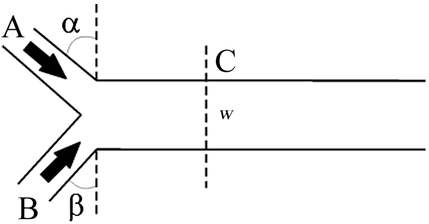
Figure 1. Suppose, for definiteness, that the red liquid is supplied into Channel A and the blue liquid into Channel B. An important factor in the mixing process is the establishment of the velocity profile in the mixing channel. Since the Reynolds number in the microchannels considered in this section is very low, the velocity profile is established not far from the channel inlet (at a distance of about 0.06
w, where
w is the width of the mixing channel; see
Figure 1).
Figure 1.
Diagram of the Y-type micromixer.
Figure 1.
Diagram of the Y-type micromixer.
If the flow rate is the same in both inlet channels, then the flow Reynolds numbers in Channels A and B are identical: Re = ρ
UQw/μ. The mixing time is determined only by the diffusion coefficient of the liquid
D: τ
m ~
w2/
D. If the mixer channel has length
L, the time required for a liquid particle to pass through the channel is τ
L ~
L/
UQ ~ (ρ
Lwh)/
Q. In this case, the mixing efficiency in the channel is determined by the ratio of these two times:
where
v = μ/ρ is the kinematic viscosity coefficient. Therefore, for a given channel and given liquids, the mixing time increases with increasing Reynolds number. If the liquids mixed in the channel are water, then in accordance with Equation (5), the mixing in a channel of length
L = 1 cm is efficient if τ
m << 10Reτ
L, which is valid only for very low Reynolds numbers. This implies, in particular, that, starting with some values of the Reynolds number, the mixing efficiency will not change. This is also confirmed by direct simulation. Indeed, at Reynolds numbers in the range of 10 to 0.01, the mixing efficiency remains virtually unchanged.
Equation (5) leads to another estimate:
which contains the diffusion Péclet number Pe =
wUQ/
D. For a given Péclet number, the mixing length
Lm ~
UQτm ~
wPe is shorter the smaller the width of the channel, and this length increases with increasing Péclet number.
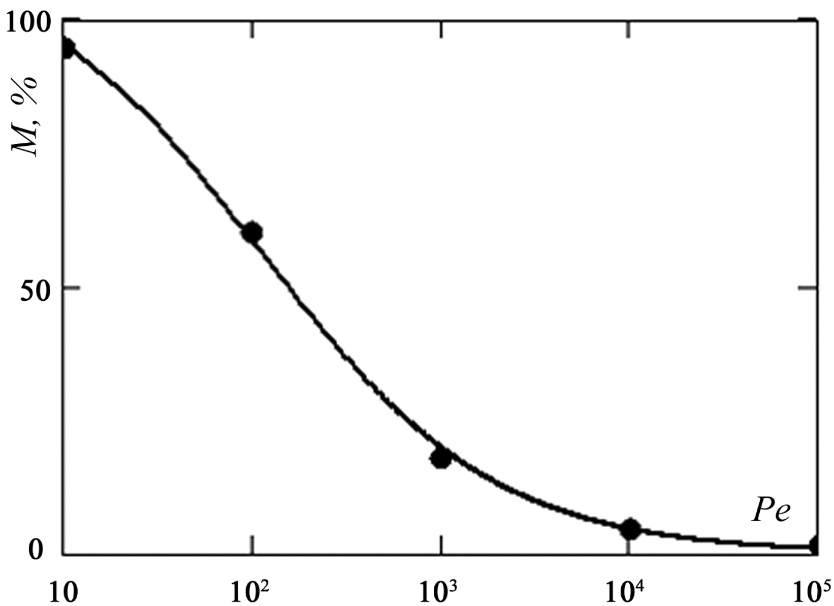
However, it should be emphasized that the dependence of the mixing efficiency on the Péclet number is nonlinear. It is presented in
Figure 2. Here, the mixing efficiency
M was determined by the formula:
where
w = 300 μm is the width of the channel in which the mixing occurs (see
Figure 1) and
C is the dye concentration in the section at a distance of 4000 μm from the site of merging of the flows. This dependence is well described by the formula:
In
Figure 2, this is shown by the continuous curve, and the points are calculation data. This dependence is, of course, conventional, as it involves, in particular, the definition of the mixing efficiency.
Figure 2.
Mixing efficiency in a Y-type mixer versus Péclet number.
Figure 2.
Mixing efficiency in a Y-type mixer versus Péclet number.
Next, consider the effect of the angles α and β on the mixing efficiency. Both angles were varied from 0° to 90° (see
Figure 1). The degree of opening of Channels A and B was found to have a weak effect on the mixing efficiency. For the mixer where two identical liquids were mixed, this difference was about 7%. In the case where the two angles were identical (symmetric mixer), the maximum efficiency was achieved for α = β = 0°. Thus, the efficiency of T-type mixers is slightly lower than that of Y-type mixers. As the angle was increased to 90°, the mixing efficiency changed from 18.2% to 17.6%. The mixing efficiency of asymmetric mixers was lower than that of symmetric mixers. For a mixer with α = 60°, β = 10°, the mixing efficiency was 17.4%, which is lower than the minimum efficiency for a symmetric mixer. These differences are somewhat larger if two different liquids are mixed. However, in all cases, symmetric mixers are more efficient at minimum angles of opening of the inlet channels. These results are predictable and are associated with changes in local Péclet numbers.
Since diffusion is an important factor in the mixing process in microchannels, a great channel length is required to provide flow mixing. Naturally, this leads to a substantial pressure drop due to friction at the channel walls. On the other hand, it is obvious that these losses are lower if the flow slip rather than no-slip condition is specified at the walls of the channel. In macroscopic descriptions, the no-slip condition is always used as the boundary condition. Slip boundary conditions are normally employed only to describe flows of rarefied gases. This is due to the fact that in gases, the characteristic wall slip length
b is of the order of the Knudsen number,
![]()
, which can be great in gases (here, the wall slip length
b is given by the condition
v =
b(∂v/∂
x), where the flow occurs along the
X-axis,
v is the flow velocity in this direction and the
Y-axis is perpendicular to the channel wall the λ-mean free path of the molecules). In macroflows of a liquid under normal conditions, the slip length ranges from a few nanometers to several tens of nanometers. This slip can be neglected. In microflows, however, this slip can be significant. In addition, the slip length in microflows can reach a few hundred nanometers. This is due to a change in the short-range order of the fluid near the surface, possible gas release at the channel walls,
etc. The presence of slip leads to a significant decrease in the frictional resistance at the channel walls and, hence, to a reduction in the pressure drop. The slip length can be increased by using various hydrophobic or even ultra-hydrophobic coatings (see, e.g., [
26,
27]). In this case, the slip length can reach tens of micrometers.
Systematic calculations of flow in Y-type micromixers were performed in [
12] to study the slip effect. The slip length was varied from 10 nm to 20 μm; the corresponding data are presented in
Table 1. Increasing the slip length to about 5 μm almost halves the pressure drop. It should be emphasized that in the presence of slip at the walls, the mixing efficiency does not change for short slip length, and even increases for great slip lengths.
Table 1.
The effect of slip at the channel walls on the pressure drop and mixing efficiency.
Table 1.
The effect of slip at the channel walls on the pressure drop and mixing efficiency.
| b (μm) | Δp (Pa) | M (%) |
|---|
| 0 | 293.3 | 17.6 |
| 0.01 | 293.1 | 17.6 |
| 0.05 | 291.7 | 17.6 |
| 0.1 | 290.1 | 17.6 |
| 1 | 263.0 | 17.7 |
| 5 | 184.5 | 17.9 |
| 20 | 87.6 | 18.4 |
So far, we have discussed the mixing of the same liquid. In practice, however, mixing of different liquids is of interest. As an example, data on the mixing of water and a different liquid in a Y-type mixer are presented in
Table 2. Water is supplied through Channel A. Because the physical characteristics of these liquids are very different, the mixing efficiency also varies widely. In particular, the parameter
M for acetone, glycerol, ethanol and isopropyl alcohol is equal to 36%, 3.1%, 18.2% and 9.4%, respectively. In this case, the pressure drop in the inlet Channels A and B is different and varies from 239.5 kPa for glycerol to 165 Pa for acetone.
Table 2.
Parameters of mixed liquids.
Table 2.
Parameters of mixed liquids.
| Liquids | Ρ (kg/m3) | Μ (Pa·s) | D (× 10−9 m2/s) |
|---|
| Acetone | 800 | 0.00029 | 4.56 |
| Glycerol | 1260 | 1.48 | 0.0083 |
| Ethanol | 790 | 0.0012 | 1.24 |
| Isopropyl alcohol | 786 | 0.0029 | 0.38 |
Equations (5)–(8) provide an estimate of the mixing time and length and, hence, the efficiency of micromixers. From general considerations, it is clear that the mixing time can be reduced considerably by multiple splitting of the mixing flow. This principle underlies the design of lamination mixers (see, for example, [
11]). A similar idea is to place a number of obstacles in mixing flow to change the flow structure, thus accelerating the mixing process. It is clear that, in laminar flow, a symmetrical arrangement of obstacles is inefficient. In addition, the characteristic size of the obstacles should be comparable to the channel size. Moreover, the mixer is easy to optimize for this parameter.
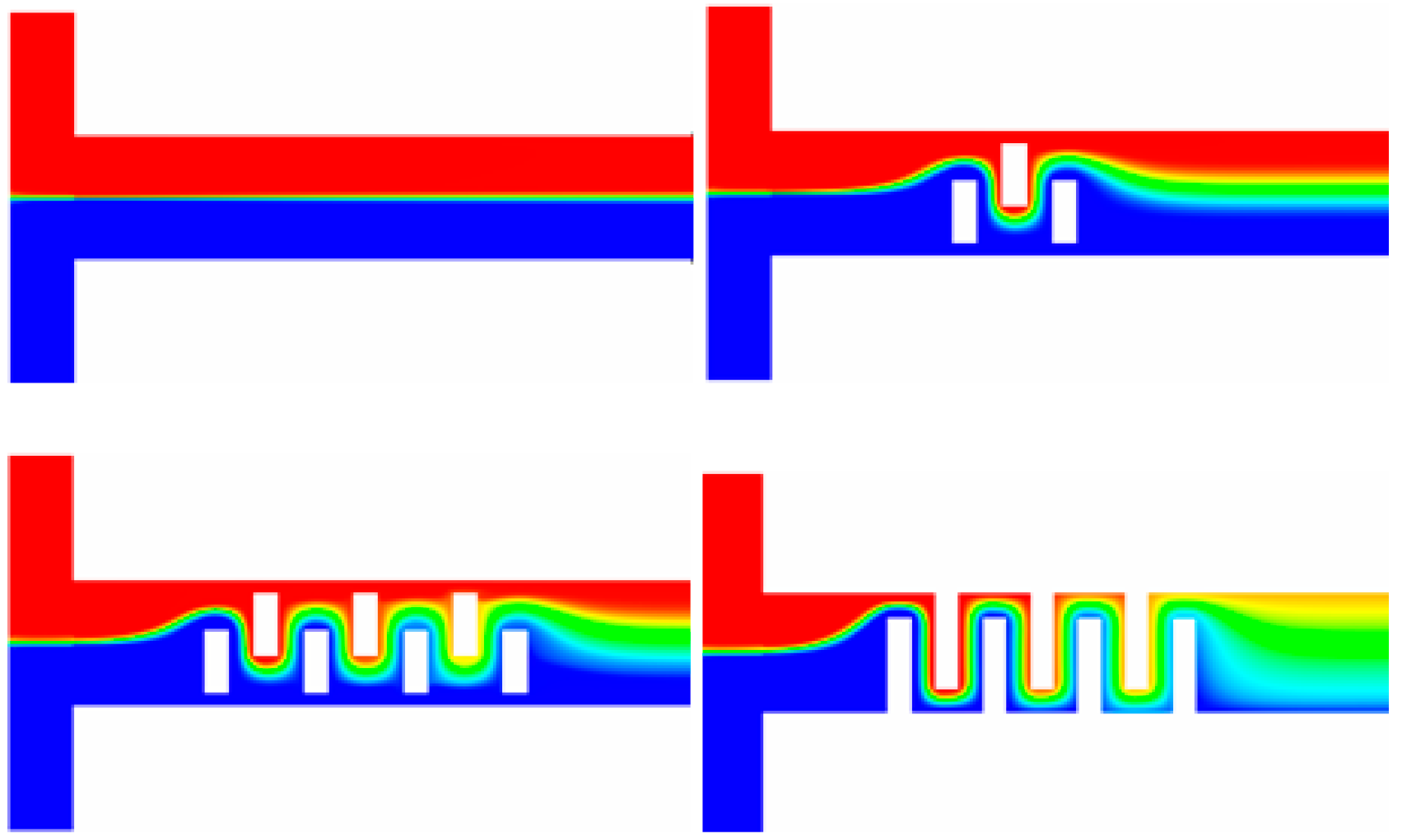
As a first example,
Figure 3 shows the mixing of two fluids in a T-type mixer with asymmetrically arranged three and seven rectangular inserts. The width of the mixing channel is 100 μm; the width of the inlet channels is 50 μm, and the height of the mixer is 50 μm. The Reynolds number is Re = 2, and the Péclet number Pe = 5 × 10
3. Since increasing the number of inserts increases the length of the channel, it is more appropriate to analyze the mixing and pressure drop characteristics normalized by the channel length, which are presented in
Table 3. Here, the first column shows the number of inserts; all inserts, except for the last line, had the same dimensions of 50 μm × 20 μm in cross-section and 50 μm in height.
Figure 3.
Comparison of the mixing of two fluids (red and blue) in a T-type mixer with straight rectangular inserts.
Figure 3.
Comparison of the mixing of two fluids (red and blue) in a T-type mixer with straight rectangular inserts.
Table 3.
Specific (per unit length) mixing efficiency and specific loss of pressure in a mixer with rectangular inserts.
Table 3.
Specific (per unit length) mixing efficiency and specific loss of pressure in a mixer with rectangular inserts.
| N | M (%/μm) | Δp (Pa/μm) |
|---|
| 0 | 0.0094 | 0.37 |
| 3 | 0.026 | 0.92 |
| 5 | 0.035 | 1.44 |
| 71 | 0.045 | 1.92 |
| 72 | 0.085 | 7.38 |
The mixing efficiency increases with increasing number of inserts, but the pressure loss also increases. This can be reduced by using hydrophobic coatings. At a slip length
b = 1 μm, the pressure drop can be reduced by 10%. The inserts in the second and third pictures are arranged in a checkerboard pattern at a certain distance from the channel walls. The mixing efficiency can be significantly improved by increasing the length of the inserts and connecting them to the channel walls. The last illustration in
Figure 3 shows mixing in such a mixer with seven inserts 70 μm × 20 μm in cross-section. The mixing efficiency it is given in the last row of
Table 3.
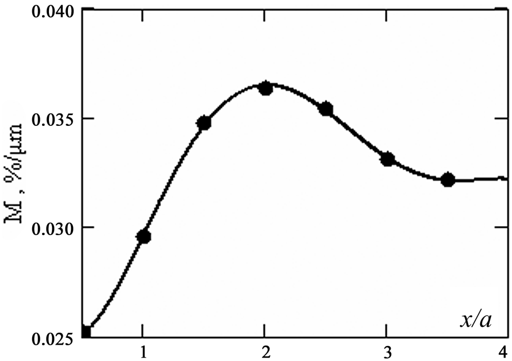
Of course, the flow topology depends strongly on the channel geometry, in particular the distance between the inserts. The mixing efficiency can be improved by varying this distance. As an example,
Figure 4 shows the dependence of the mixing efficiency in a channel with five rectangular inserts on the dimensionless width of the insert
a, which is equal to 20 μm. The cross-section of the inserts is 50 μm × 20 μm, and the flow characteristics are the same as in
Figure 3. This mixer works best when the distance between the inserts is about 2
а. Increasing the distance between the inserts monotonically decreases the pressure drop. Thus, the pressure drop can be reduced by twenty-five percent by increasing the distance between the inserts from
a to 2
a. On the other hand, the wall slip in this micromixer has a significantly weaker effect on the pressure drop than in the smooth channel.
Finally, it should be noted that the optimization of the mixing parameters of a micromixer generally depends on the Reynolds and Péclet numbers. However, as noted above, the mixing efficiency is practically independent on the Reynolds number over a wide range of Re (at Re ≤ 1), and it begins to grow only at Re > 1. The mixing efficiency depends weakly on the Péclet number starting with values Pe ~ 103. On the other hand, as the Péclet number changes from 10 to 1000, the mixing efficiency changes by about an order of magnitude.
Figure 4.
Normalized mixing efficiency in a mixer with five rectangular inserts versus dimensionless distance between them.
Figure 4.
Normalized mixing efficiency in a mixer with five rectangular inserts versus dimensionless distance between them.
4. Fluid Mixing at Moderate Reynolds Numbers
Higher Reynolds number flows in micromixers have been actively studied in the last decade. The greatest attention has been focused on flow in T-type micromixers. In this case, a complex vortex flow arises in the microchannel, which is characterized by the formation of so-called Dean vortices. Engler
et al. [
28] have experimentally demonstrated the existence of a critical Reynolds number at which Dean vortices in microchannels lose symmetry. It has been found that for a 600 μm × 300 μm × 300 μm channel, the critical Reynolds number is about 150. The critical Reynolds number has been shown to be strongly dependent on the channel dimensions. Telib
et al. [
29] have performed a numerical simulation of transitional flow regimes (at Reynolds numbers Re = 300 ÷ 700), but mixing processes have not been studied. Experimental and numerical studies of the mixing of two liquids at Reynolds numbers from 50 to 1400 have been made by Wong
et al. [
30]. The existence of an unsteady periodic regime for some Reynolds number was first demonstrated numerically by Gobert
et al. [
31]. The most comprehensive experimental study of mixing in T-type microchannels at moderate Reynolds numbers (100–400) was presented by Hoffmann
et al. [
11]. Here, the velocity and concentration fields in different sections of the mixer have been investigated using laser-induced fluorescence (µLIF) and micro-particle image velocimetry (micro-PIV) measurements. The mixing efficiency was first measured.
Finally, a mention should be made of a series of computational and experimental studies [
32,
33,
34], where, in particular, some flow regimes in T-shaped microchannels were calculated. A number of characteristic flow regimes were found, and the flow structure in them were studied. The mixing efficiency was calculated. The calculated and experimental mixing patterns were compared qualitatively, and the distribution of the mixing efficiency along the channel was calculated.
Systematic data on the flow and mixing regimes in such micromixers were obtained in [
22,
35]. In the present study, a hydrodynamic simulation was performed for various flow regimes in a T-type micromixer at Reynolds numbers Re = (ρ
Uh/μ) from one to one thousand. Here,
U =
Q/(2ρ
dh2);
d = 100 μm is the height of the channel, and
h = 133 μm is the hydraulic diameter. The cross-section of the mixing channel was 100 μm × 200 μm, and its length was 1500 μm. The inlet channels were symmetric and perpendicular to the mixing channel; their cross-section was 100 μm × 100 μm, and the total length was 800 μm. Pure water was supplied through the left inlet and water dyed with rhodamine through the right inlet. The flow rate
Q was the same in both cases. The two liquids had the same density and viscosity coefficient of 1000 kg/m
3 and 0.001 Pa·s, respectively. The diffusion coefficient of the dye in water was
D = 2.63 × 10
−10 m
2/s. Thus, for the problem under consideration, the Schmidt number
Sc = μ/(ρ
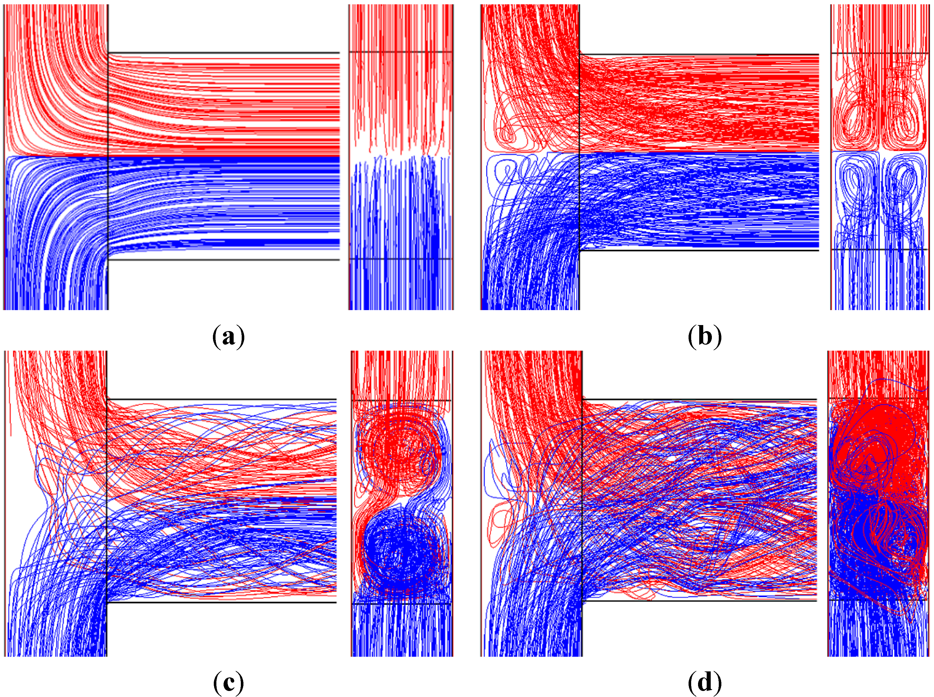
D) is 3800. This implies that the thickness of the hydrodynamic boundary layer is much greater than the thickness of the diffusion boundary layer. Thus, to obtain reliable numerical results, it is necessary to use fine computational grids providing high resolution of the mixing layer. The calculation was performed on a two-block grid consisting of 9.8 million nodes (140 nodes across the width of the mixing channel, 70 nodes along the height and 1000 nodes along the length). As a result, five different flow regimes were found to exist, each of which developed at certain Reynolds numbers. At low Reynolds numbers (Re < 5), steady irrotational flow occurs in the mixer. Mixing in this case is due to ordinary molecular diffusion, and the mixing efficiency is rather low (see the previous section). The flow structure in the longitudinal and cross-sections of the mixer can be visualized using marker particle trajectories. For low Reynolds numbers, it has the form shown in
Figure 5a.
As the Reynolds number is increased, two steady symmetric horseshoe vortices, called Dean vortices, are formed at the inlet of the mixing channel. The resulting vortex structure is best represented in three projections in terms of the isosurface of the quantity λ
2. Here, λ
2 is the second eigenvalue of the tensor (
D:D + Ω:Ω), where:
is the vorticity tensor,
D is the strain rate tensor. The structure of the vortices formed for flow at a Reynolds number Re = 120 is shown in
Figure 6.
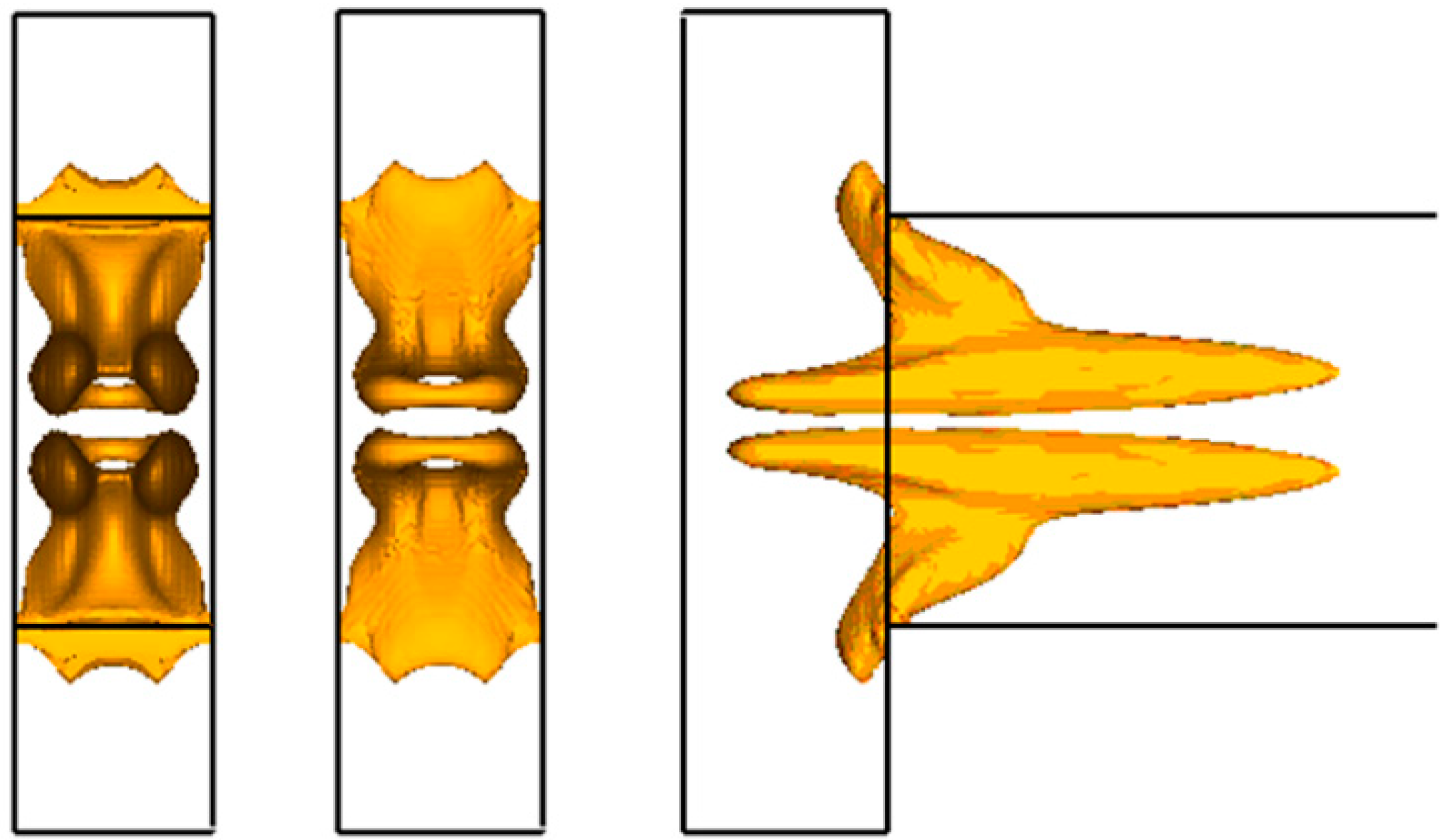
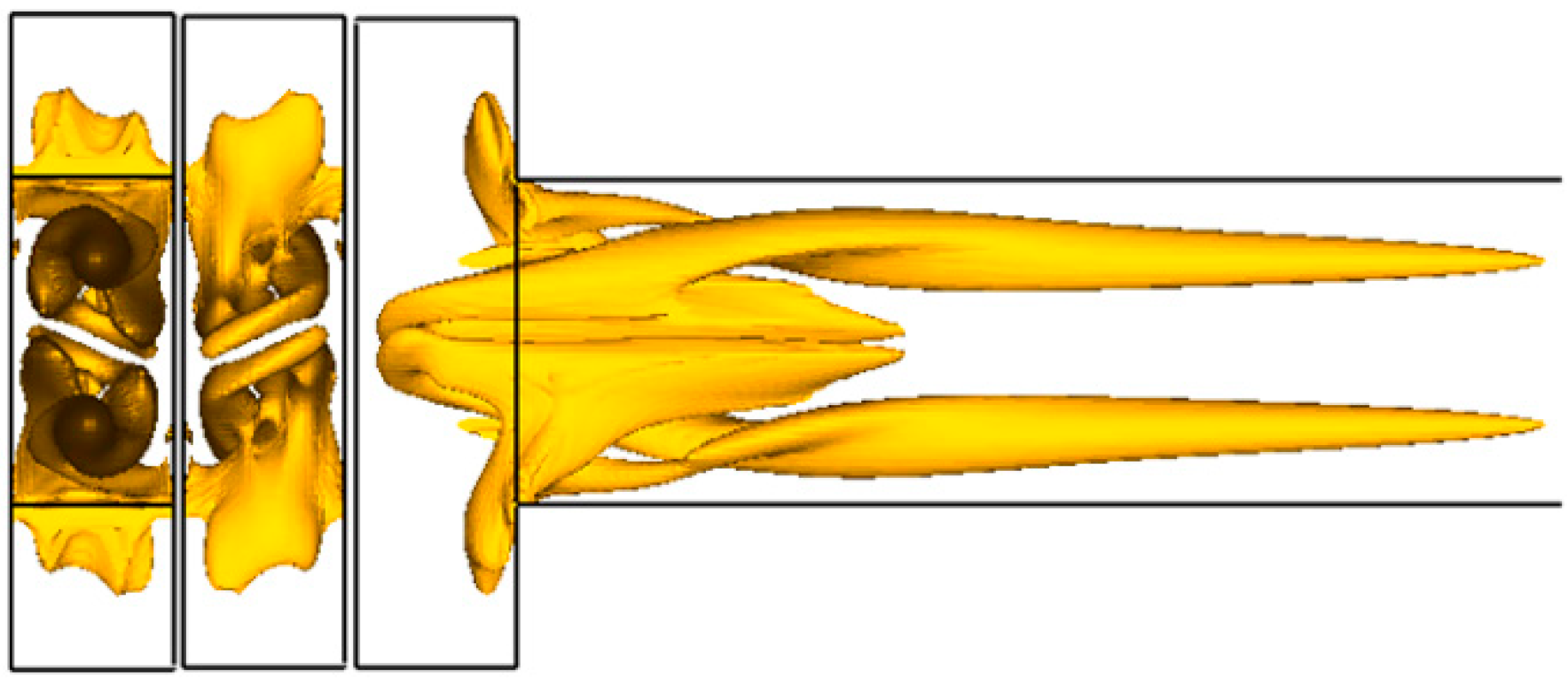
Horseshoe vortices result from the secondary flows caused by the centrifugal force arising from the turning of the flow. The evolution of the structure of the developing velocity field with increasing Reynolds number is shown in
Figure 7. Here,
Figure 7a,b correspond to Reynolds numbers of 20 and 120. The vortices formed at the inlet of the mixing channel dissipate and move along the channel. The dissipation of the vortices is due to the viscosity of the liquid, and therefore, the dissipation rate decreases with increasing Reynolds number. For flow at a Reynolds number Re = 120 (see
Figure 7b), the horseshoe vortices decay in the mixing channel at a distance of about 400 mm from the inlet section; whereas at Re = 20 (
Figure 7a), this distance is about 70 μm. This implies that the intensity of the Dean vortices increases with increasing Reynolds number. In addition, their configuration changes (
cf.
Figure 7a,b).
The occurrence of Dean vortices is a threshold phenomenon, and the corresponding Reynolds number is generally determined by the size of the channel and can be characterized by the critical Dean number
![]()
[
36], where
R is the radius of curvature of the flow turning. In the channel studied in this work, Dean vortices were observed at Re ≈ 20. If the radius of the flow turning in this microchannel is set equal to
R = d/2, this corresponds to a critical Dean number
Dn = 28.
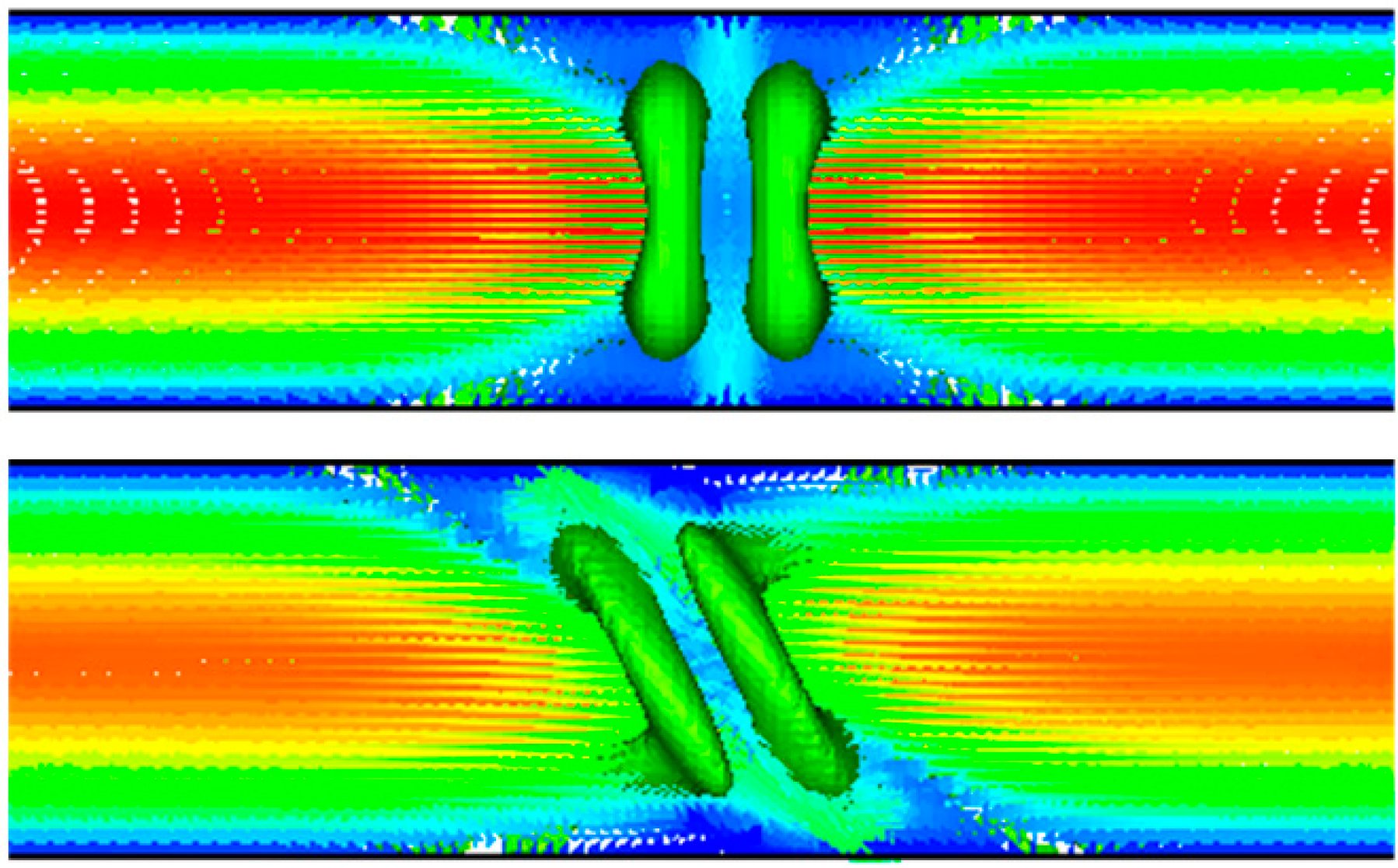
Continuing to increase the Reynolds number, we observe a very interesting change in the flow regime. Starting at a Reynolds number of about 150, the pair of horseshoe vortices abruptly rotates at an angle of 45° about the central longitudinal plane of the mixer, due to the development of Kelvin−Helmholtz instability. This restructuring is clearly seen in
Figure 8, where the flow is represented in terms of the isosurface of λ
2. Here the top figure corresponds to Re = 120, and the bottom figure to Re = 186 (higher than the critical value at which the restructuring occurs). This flow restructuring is clearly seen in
Figure 6c and
Figure 7 (see also
Figure 5c).
Figure 5.
Marker particle trajectories in a T-type micromixer at various Reynolds numbers: (a) Re = 1, (b) Re = 120, (c) Re = 186 and (d) Re = 600.
Figure 5.
Marker particle trajectories in a T-type micromixer at various Reynolds numbers: (a) Re = 1, (b) Re = 120, (c) Re = 186 and (d) Re = 600.
Figure 6.
Vortices formed at the inlet of the mixing channel. Re = 120. Front view (left), a rear view (center) and a side view with a vertical section of the channel (right).
Figure 6.
Vortices formed at the inlet of the mixing channel. Re = 120. Front view (left), a rear view (center) and a side view with a vertical section of the channel (right).
Figure 7.
Velocity field in the cross-section of the mixing channel at a distance of 100 μm from the inlet for various Reynolds numbers: (a) Re = 20, (b) Re = 120 and (c) Re = 186.
Figure 7.
Velocity field in the cross-section of the mixing channel at a distance of 100 μm from the inlet for various Reynolds numbers: (a) Re = 20, (b) Re = 120 and (c) Re = 186.
Figure 8.
Velocity field in the cross-section of the mixer (end view) and the isosurface of λ2: (top) Re = 120 and (bottom) Re = 186.
Figure 8.
Velocity field in the cross-section of the mixer (end view) and the isosurface of λ2: (top) Re = 120 and (bottom) Re = 186.
Kelvin–Helmholtz instability leads to the formation of diagonal shear flow in the cross-section of the channel. The center of symmetry of the flow becomes the central longitudinal line through the mixing channel. As a result, instead of four vortices (
Figure 7b), as was the case for the symmetric flow regime (Re < 150), two intense vortices with the same direction of vorticity are formed in the cross-section, even at a distance of about 400 μm from the inlet of the mixing channel (
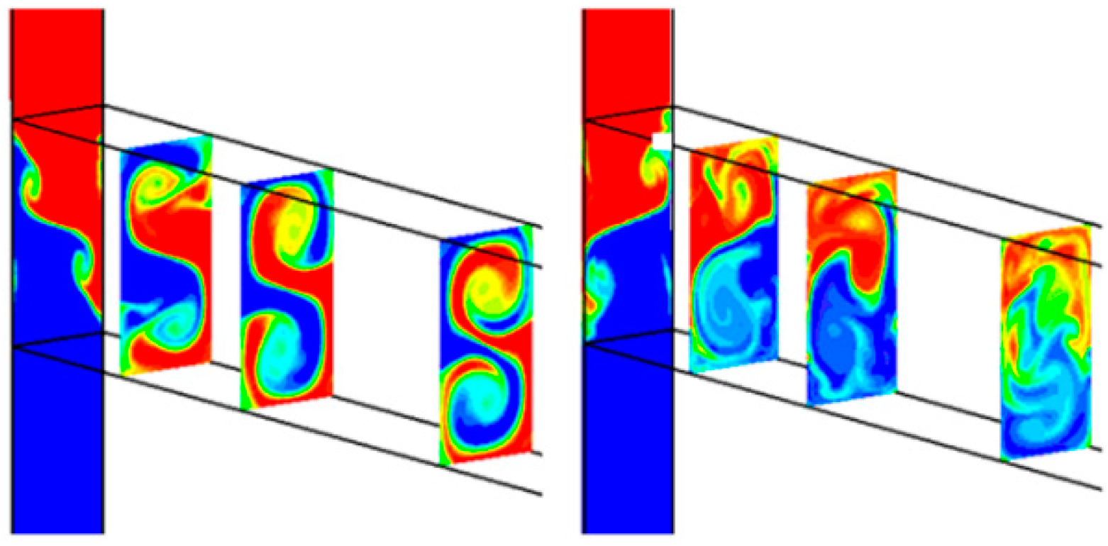
Figure 7c). The flow has an S-shaped vortex structure, which is especially clearly seen at the left in
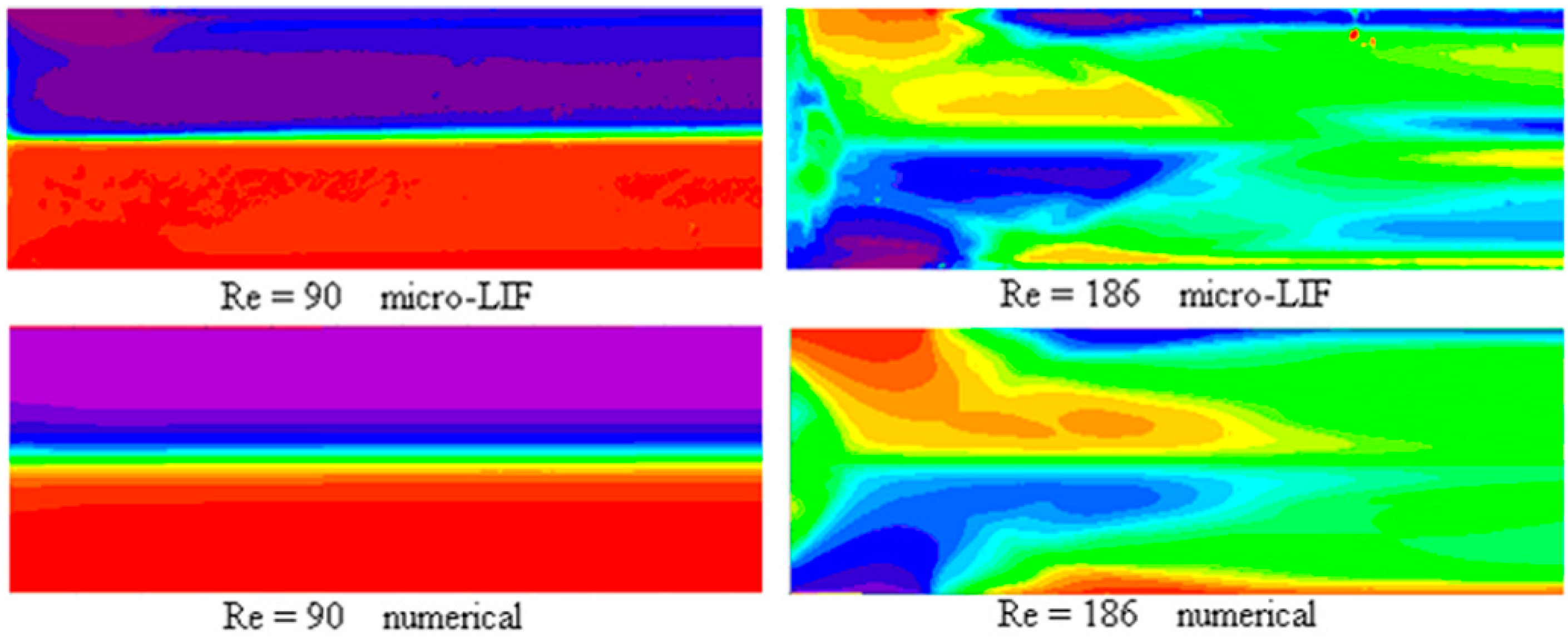
Figure 9. Here, mixing is shown by dye concentration isolines in four cross-sections of the mixer. The first section on the left is located at the inlet of the mixing channel, the second at a distance of 100 μm from the inlet, the third at a distance of 200 μm and the fourth at 400 μm. In the Figure, the red color corresponds to pure water, and the blue color to water dyed with rhodamine. This flow regime is also steady and is observed up to a Reynolds number of 240. The structure of this flow is illustrated in
Figure 10, where the flow developing in the mixing channel at Re = 186 is shown in terms of the λ
2-isosurface.
In the symmetric flow regime (Re < 150), the vortices compensate each other, and the total hydrodynamic moment is zero. In the asymmetric unsteady regime, the hydrodynamic moment of the flow is different from zero, since the vortices in the S-shaped structure rotate in the same direction. Naturally, the total mechanical moment in the system is conserved in both cases, because in the asymmetric regime, a compensating moment occurs on the channel walls. Finally, it should be noted that the vortex intensity in the asymmetric regime is significantly higher than that in the symmetric one. Therefore, despite dissipation, these vortices are observed along the entire length of the mixer.
The occurrence of S-shaped vortices has been observed in previous experiments [
11].
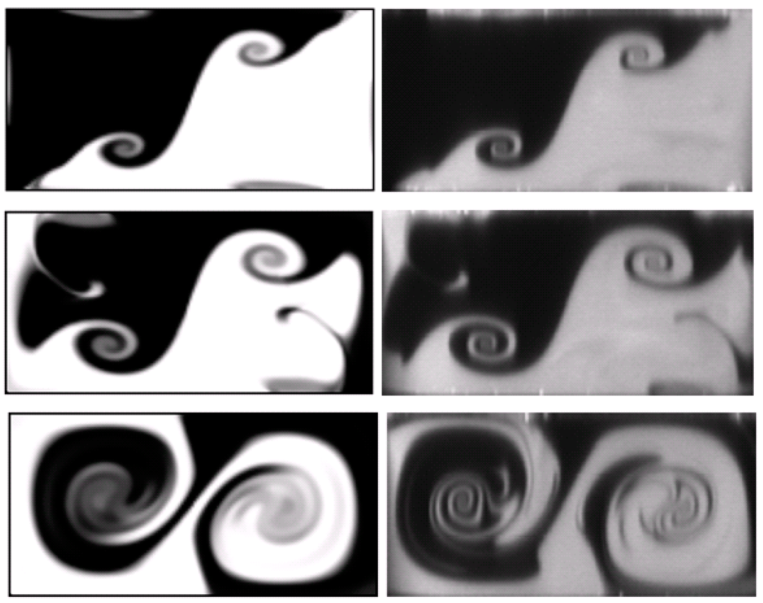
Figure 11 shows a comparison of the results of visualization of experiment [
11] and calculation [
35] at Re = 186 in three different sections of a micromixer. The experiment was performed for the same micromixer using laser-induced fluorescence (µLIF). The top figures show the concentration distribution of the mixing components at the inlet cross-section of the mixing channel, the middle figures at a distance of 1000 μm from the inlet and the bottom figures at the outlet of the mixer. As can be seen, there is good agreement between the calculated and experimental shapes of the liquid interface.
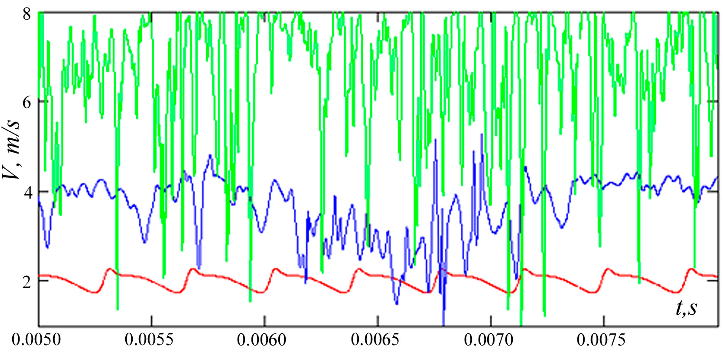
The steady asymmetric flow regime described here is observed at Reynolds numbers from 140 to 240. Starting at a Reynolds number of about 240, the flow ceases to be steady. In the Reynolds number range 240 < Re < 400, a periodic flow regime occurs. This implies, in particular, that the flow velocity is also a periodic function of time. In
Figure 12, the lower curve corresponds to this flow regime.
Figure 9.
Mixing process in the micromixer at different Reynolds numbers: (left) Re = 186 and (right) Re = 600.
Figure 9.
Mixing process in the micromixer at different Reynolds numbers: (left) Re = 186 and (right) Re = 600.
Figure 10.
Vortices formed at the inlet of the mixing channel. Re = 186. Front view (left), a rear view (center) and a side view with a vertical section of the channel (right).
Figure 10.
Vortices formed at the inlet of the mixing channel. Re = 186. Front view (left), a rear view (center) and a side view with a vertical section of the channel (right).
Figure 11.
Dye concentration isolines in different cross-sections of the mixer at Re = 186. Results of calculations (
left) and laser-induced fluorescence (µLIF) measurements (
right) [
11].
Figure 11.
Dye concentration isolines in different cross-sections of the mixer at Re = 186. Results of calculations (
left) and laser-induced fluorescence (µLIF) measurements (
right) [
11].
Figure 12.
Change in the flow velocity at the outlet of the mixing channel with time. The lower curve corresponds to Re = 300, the middle curve to Re = 600 and the upper curve to Re = 1000.
Figure 12.
Change in the flow velocity at the outlet of the mixing channel with time. The lower curve corresponds to Re = 300, the middle curve to Re = 600 and the upper curve to Re = 1000.
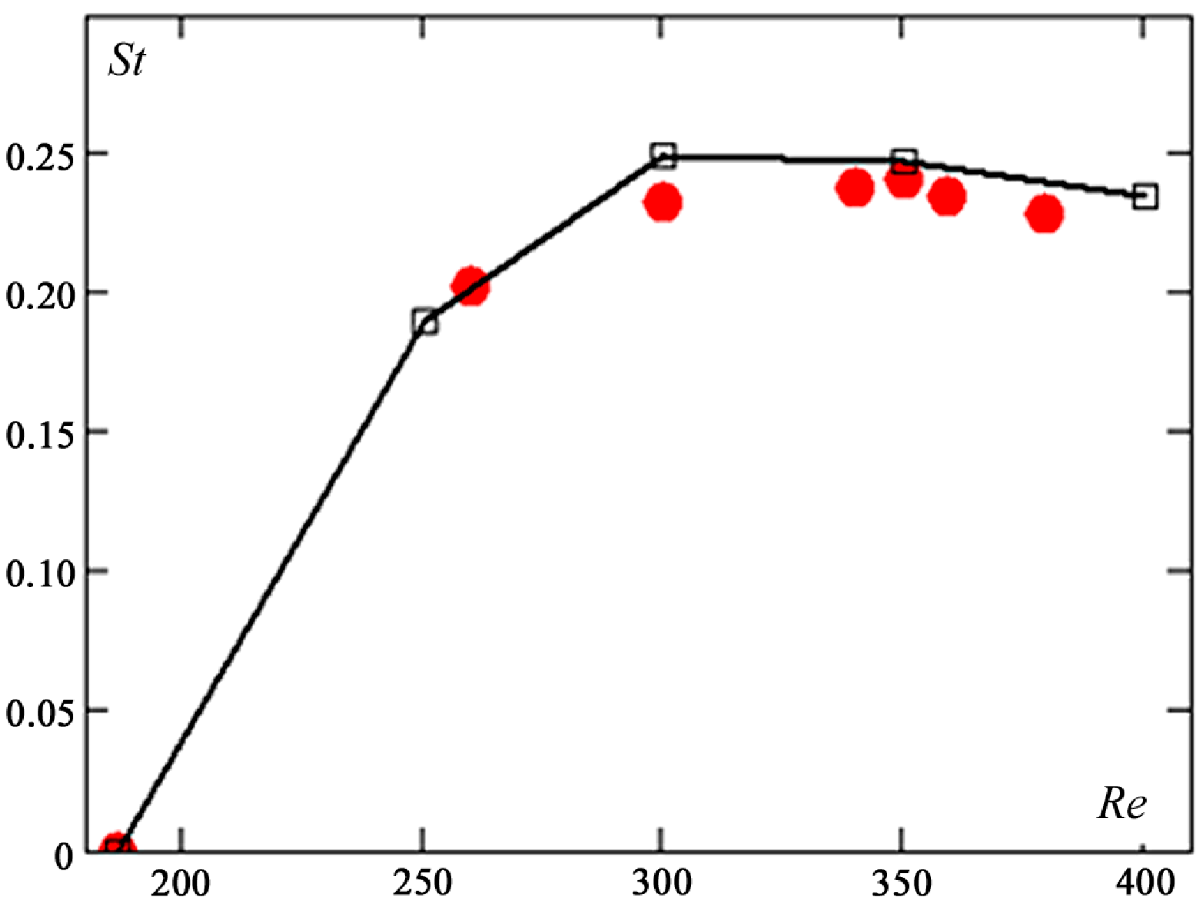
The flow oscillation frequency
f depends on many factors: the channel geometry, the liquid viscosity and the Reynolds number. This dependence can be characterized by the Strouhal number
St = (
fd2)/(
vRe), which, in fact, is the dimensionless frequency of flow oscillations normalized by the Reynolds number. A plot of the Strouhal number
versus Reynolds number is shown in
Figure 13 (square points). The oscillation frequency increases monotonically to Re = 300 and then decreases slightly. Here, the results of our calculations are in good agreement with experimental data [
32] (filled points in
Figure 13). Maximum differences are observed at high Reynolds numbers, but it should be noted that the experimental data were obtained for a channel with a cross-section of 600 μm × 300 μm.
Figure 13.
Strouhal number versus Reynolds number in steady periodic flows in the mixing channel.
Figure 13.
Strouhal number versus Reynolds number in steady periodic flows in the mixing channel.
Starting at a Reynolds number of about 450, the strict periodicity of the flow oscillations is lost. The flow first becomes quasiperiodic (450 < Re < 600) and then almost chaotic (Re > 600). The frequency spectrum of the velocity field becomes sufficiently filled and close to the continuous one. This is clearly seen in
Figure 12, where the middle curve corresponds to a Reynolds number Re = 600 (see also
Figure 9) and the upper curve to Re = 1000.
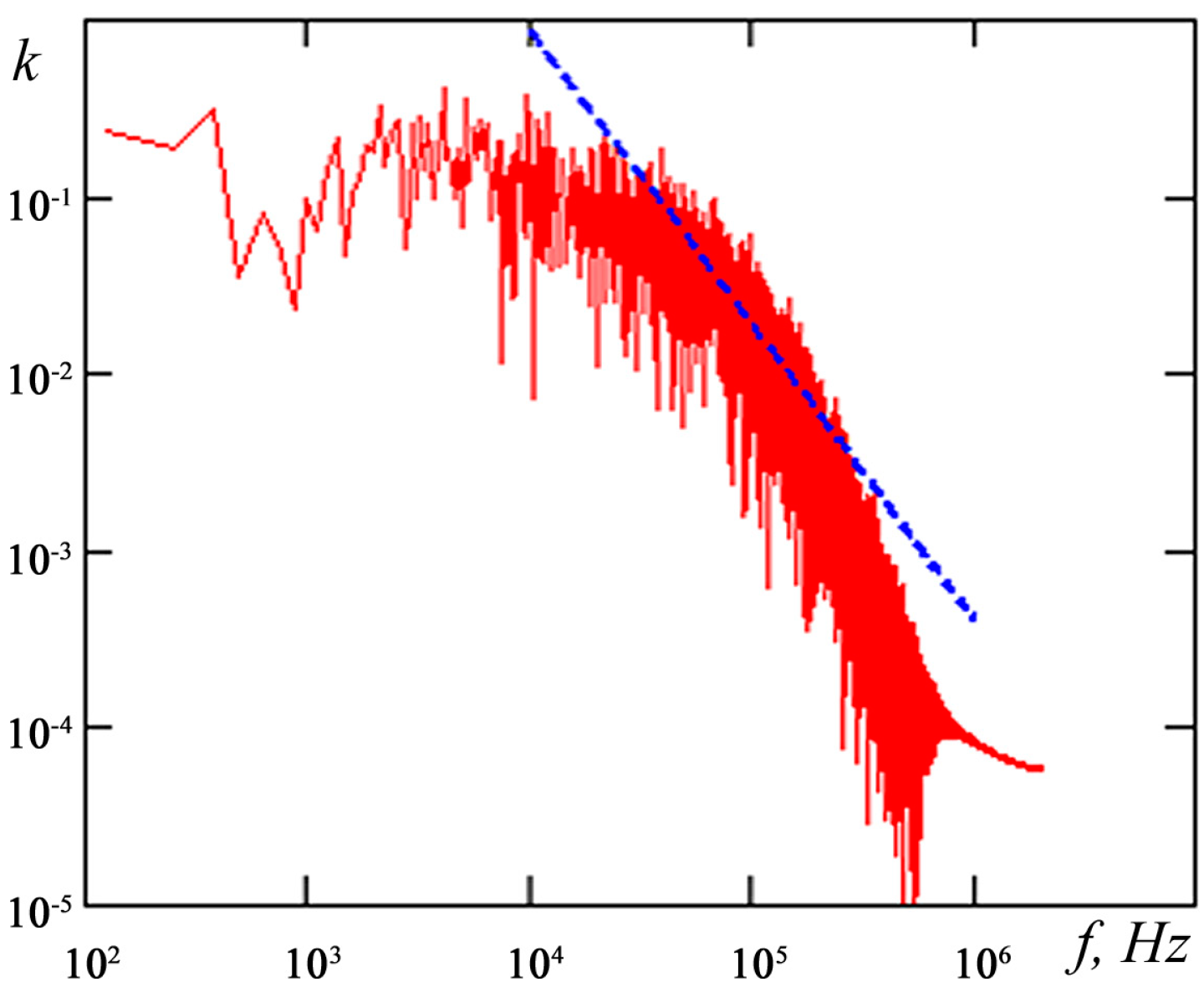
The frequency distribution of the kinetic energy of flow fluctuations
k for Re = 600 is shown in
Figure 14. This spectrum was obtained for the point located in the center of the mixing channel at a distance of 400 μm from the inlet. The dashed straight line in the plot represents the universal Kolmogorov-Obukhov law. Although the spectrum for Re = 600 cannot be considered completely continuous, as in the case of developed turbulent flow, it contains a large number of frequencies and an inertial interval, which at least suggests a transitional flow regime. That early (for channel flows) onset of turbulence is due to the development of Kelvin–Helmholtz instability in the inlet section of the mixing channel. Nevertheless, calculations show that if the mixing channel is long enough, then with increasing distance from the site of confluence of the flows, the pulsations gradually decay, the flow becomes laminar and, as expected, a steady laminar velocity profile is established.
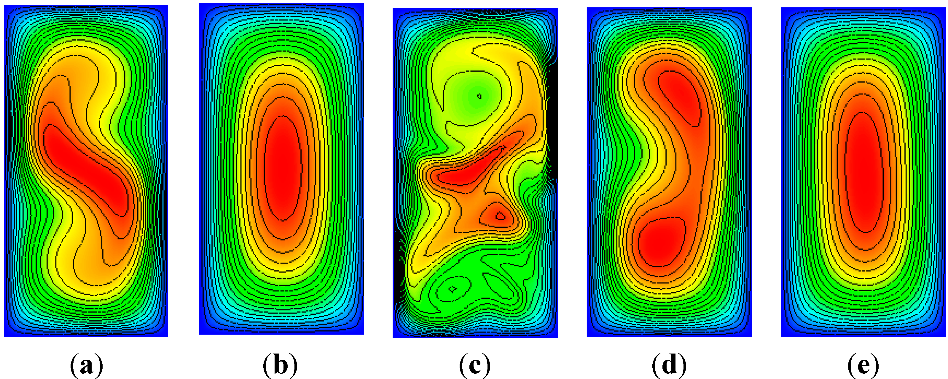
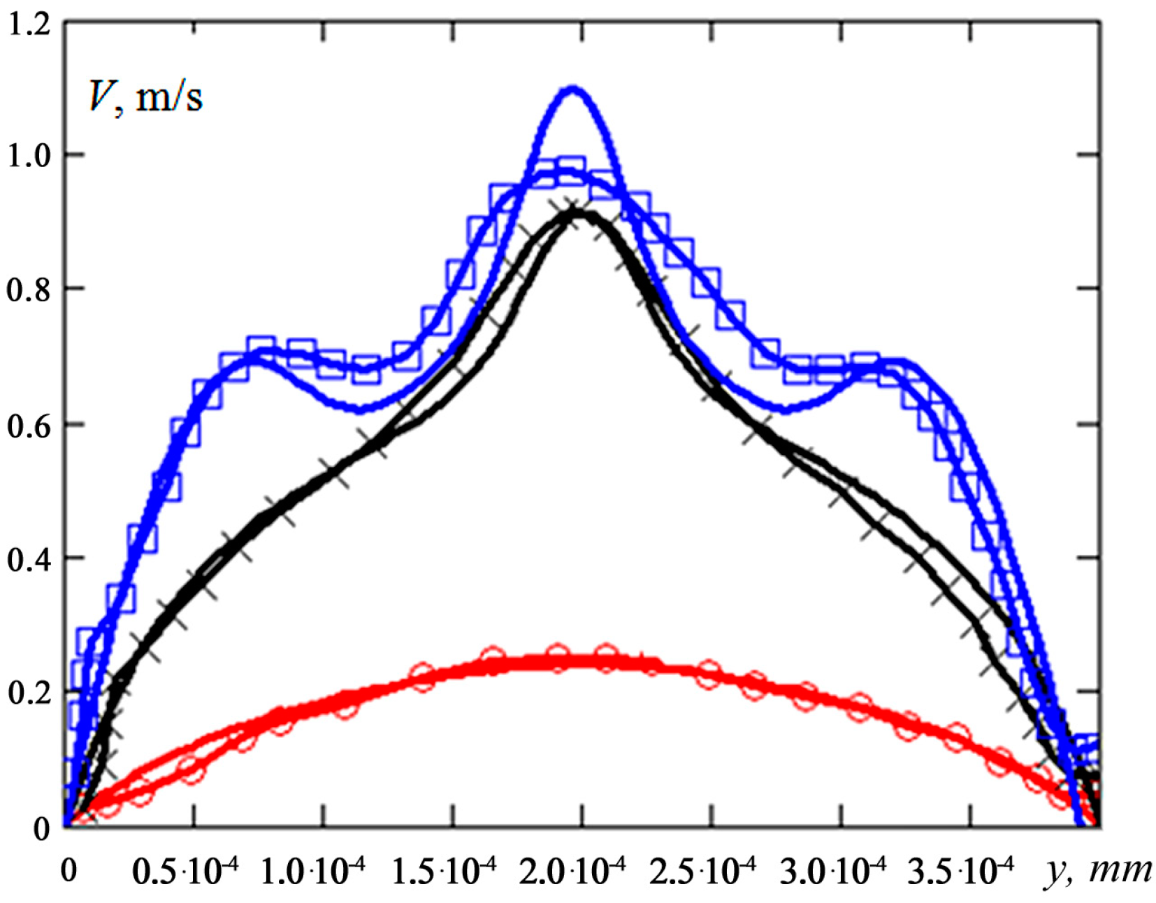
The length of establishment of the velocity profile, of course, depends on the Reynolds number. To show this, we solved the problem for a channel 7000 μm long. The data obtained are shown in
Figure 15, which compares the velocity profiles for two Reynolds numbers: Re = 186 (
Figure 15a,b) and Re = 600 (
Figure 15c–e). A laminar velocity profile is established in both cases; however, at Re = 186, the flow establishment length is close to 3500 μm, and at Re = 600, it is 7000 μm.
Figure 14.
Kinetic energy spectrum of velocity fluctuations at Re = 600.
Figure 14.
Kinetic energy spectrum of velocity fluctuations at Re = 600.
Figure 15.
Velocity magnitude in different sections of the mixing channel: (a) Re = 186, L = 500 μm; (b) Re = 186, L = 3.5 mm; (c) Re = 600, L = 500 mm; (d) Re = 600, L = 3500 mm; and (e) Re = 600, L = 700 μm.
Figure 15.
Velocity magnitude in different sections of the mixing channel: (a) Re = 186, L = 500 μm; (b) Re = 186, L = 3.5 mm; (c) Re = 600, L = 500 mm; (d) Re = 600, L = 3500 mm; and (e) Re = 600, L = 700 μm.
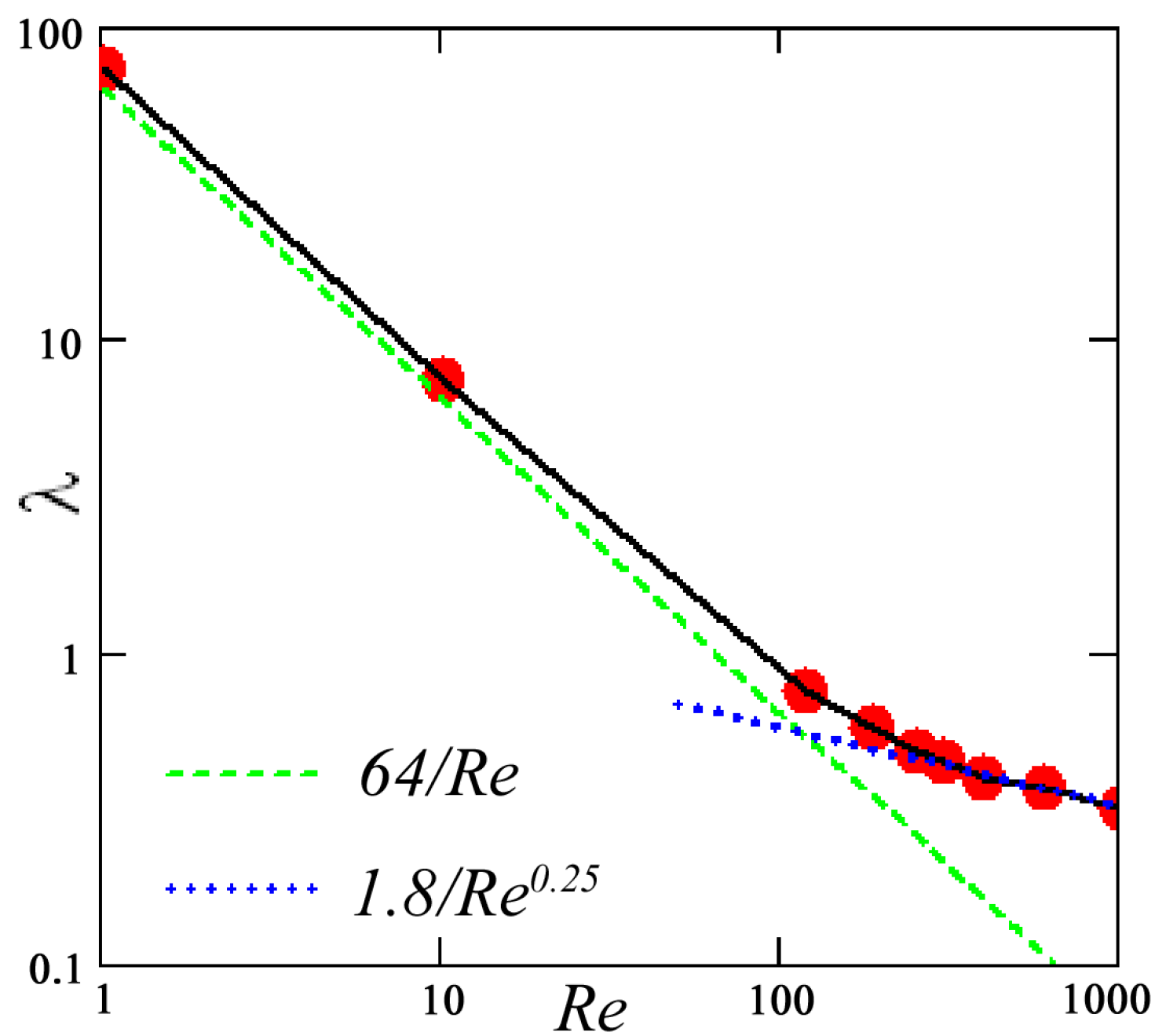
A plot of the friction coefficient λ of the mixing channel
versus Reynolds number for this mixer is given in
Figure 16. This coefficient was determined by the formula λ = (2∆
Pd)/(ρ
U2L), where ∆
P is the pressure drop in the channel and
L is the length of the channel. Filled points and the line connecting them correspond to the calculation. For comparison with the calculated results, the dashed line in the plot shows the values of the friction coefficient for steady laminar flow in a rectangular channel with a height-to-width ratio of 0.5. In this case, the friction coefficient is close to 64/Re. However, analysis shows that for low Reynolds numbers, the friction coefficient in the micromixer is on average 20%–30% higher than the friction coefficient for the steady flow.
Then, the friction coefficient values sharply deviate from the relation λ = 64/Re, indicating a laminar-turbulent transition. The calculated data on the friction coefficient in the micromixer at moderate Reynolds numbers are well described by the relation λ = 1.8/Re
0.25. The obtained value of the friction coefficient is almost six times higher than the classical Blasius relation (λ = 0.316/Re
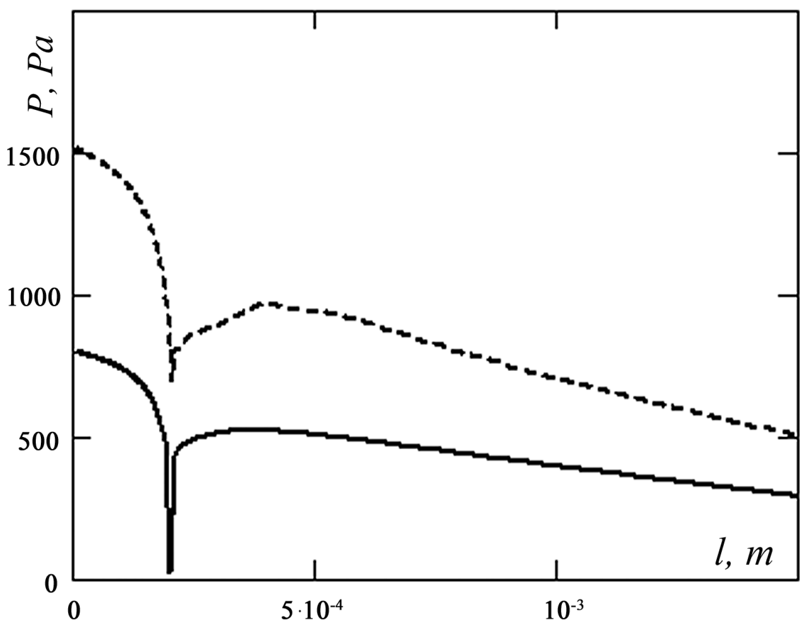
0.25) for developed turbulent flow in a straight channel. This large difference is due to flow turning at the channel inlet and flow swirling in the mixing channel. In particular, the pressure change along the channel is not monotonic. The pressure change for the two Reynolds numbers can be seen in
Figure 17. Here, the lower curve corresponds to a Reynolds number of 120 and the upper curve to 186.
Figure 16.
Friction coefficient versus Reynolds number in the mixing channel.
Figure 16.
Friction coefficient versus Reynolds number in the mixing channel.
Figure 17.
Pressure distribution on the mixer walls.
Figure 17.
Pressure distribution on the mixer walls.
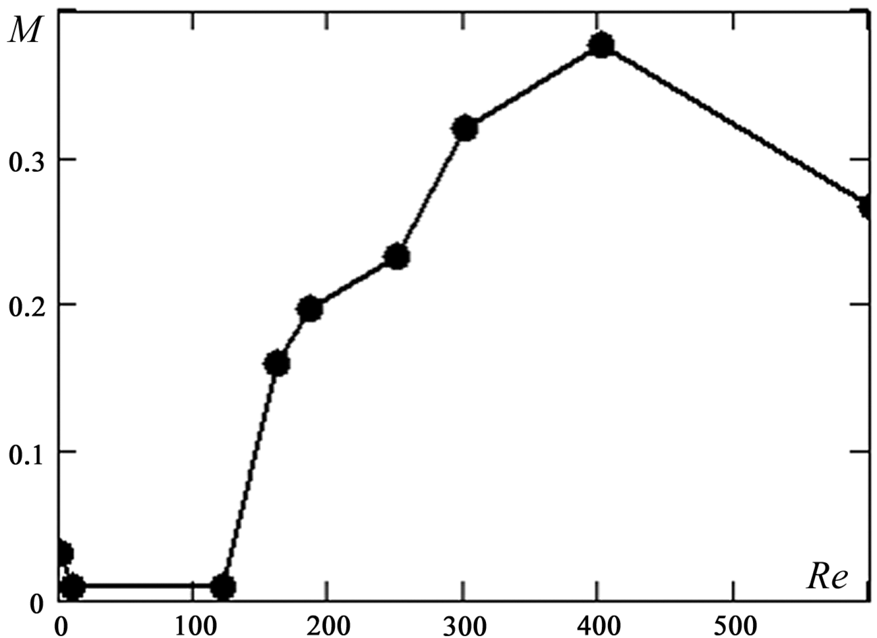
At high Reynolds numbers, the flow and mixing process are substantially three-dimensional. In this case, it is convenient to describe the mixing efficiency by using the following parameter:
is the variance of the concentration in the volume of the mixer V (
f is the component concentration,
![]()
is its average value, and
![]()
).
As already noted, at low Reynolds numbers (Re < 5), the flow in the mixer is steady and irrotational. Mixing in this case is due to ordinary molecular diffusion, and the mixing efficiency is rather low (approximately 3%; see
Figure 18.). Increasing the Reynolds number leads to the formation of steady Dean vortices. These horseshoe vortices are symmetric about the central longitudinal plane of the mixer. Each of these vortex horseshoes is within the same liquid and does not cross the interface between the media being mixed, so that this interface remains almost flat. Since the diffusion Péclet number increases with increasing Reynolds number, the mixing efficiency in this case is even lower than that in the irrotational flow (see
Figure 18) and remains low up to Reynolds numbers of about 150.
Figure 18.
Mixing efficiency versus Reynolds number.
Figure 18.
Mixing efficiency versus Reynolds number.
The loss of symmetry of Dean vortices and the formation of the S-shaped vortex structure lead to a qualitative change in the mixing pattern. The contact surface of the mixing liquids increases significantly, resulting in a considerable increase in the mixing efficiency. The mixing efficiency increases by a factor of 25 (see
Figure 18) in the flow transition from the symmetric (Re < 150) to the asymmetric (Re > 150) regime.
The onset of turbulence leads to the breakdown of the S-shaped vortex structure that formed in the mixing channel at Re > 150 and existed in the unsteady regime (see
Figure 9, which shows the evolution of the S-shaped vortex structure at Re = 600). The flow breaks up into a set of large vortices. This leads to a decrease in the contact area of the liquids mixed and a sharp reduction in the mixing efficiency (M = 26% at Re = 600). Naturally, with a further increase in the Reynolds number, the large vortex structures break up into many small vortices, which provide very good mixing of the flow. Thus, the mixing efficiency in the developed turbulent flow will far exceed the laminar value.
Usually, the length of the mixer should be large enough to provide effective mixing. Naturally, this leads to significant pressure losses due to friction at the walls. On the other hand, these losses can be reduced by using hydrophobic or even ultra-hydrophobic coatings. In microflows, the slip length can reach tens of micrometers. As shown in the previous section, the mixing efficiency did not virtually change in this case if the flow Reynolds number was small. However, the situation is different at moderate Reynolds numbers. The wall slip effect leads to a significant change in the flow conditions.
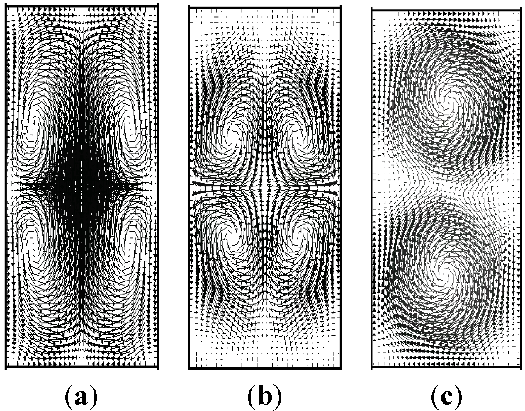
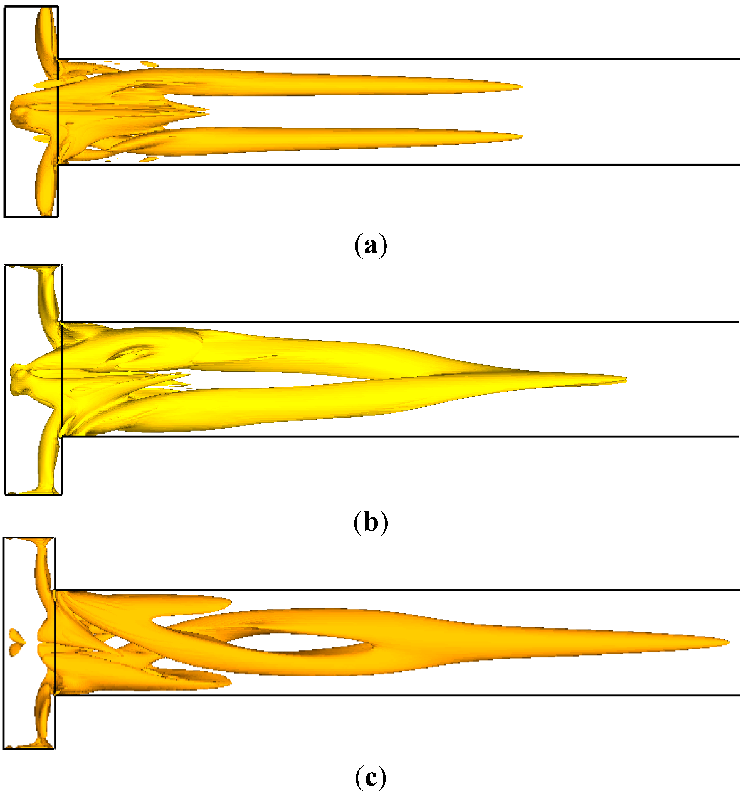
Figure 19 [
26] shows the flow structure for a Reynolds number Re = 186 and various values of the slip length
b. As already mentioned, a two-vortex structure is formed if the slip conditions are satisfied (
Figure 19a). However, for large values of the slip length, this structure is transformed into a single-vortex structure (see
Figure 19b,c). Naturally, the mixing efficiency also increases in this case. For the mixer considered here, this increase is about 30%. On the other hand, the pressure drop decreases monotonically with increasing slip length (for the investigated mixer, the decrease is approximately 30%–40%). Therefore, the flow regime can be controlled by using the no-slip condition (hydrophobic coatings).
Figure 19.
Vortex flow structure in the micromixer for different slip lengths b. Re = 186. (a) b = 0, (b) b = 10 μm and (c) b = 30 μm.
Figure 19.
Vortex flow structure in the micromixer for different slip lengths b. Re = 186. (a) b = 0, (b) b = 10 μm and (c) b = 30 μm.
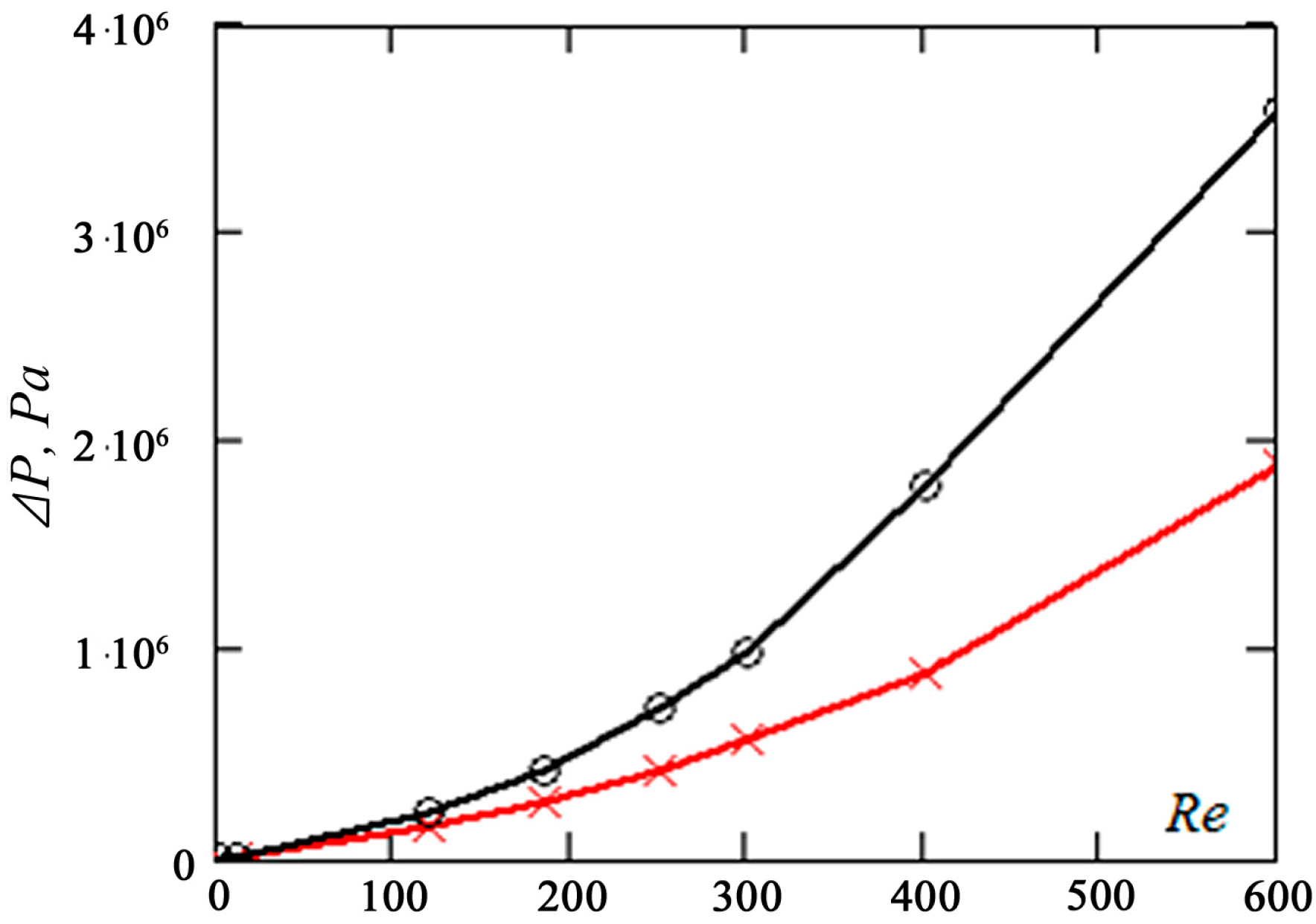
In practice, the presence of roughness on the walls can significantly change the microflow pattern. In the series of calculations presented below, periodic roughness in the form of rectangular projections was specified on the top and bottom side walls. The roughness elements were 4 μm high and 2 μm wide and spaced 10 μm apart; in another series of calculations, the roughness width was specified randomly and varied between 1 and 5 μm. The presence of roughness significantly changed the hydraulic resistance of the mixing channel.
Figure 20 shows the dependence of the pressure drop on the Reynolds number. The upper curve corresponds to a rough channel, and the lower curve to a smooth channel. At low Reynolds numbers, the resistance remains virtually unchanged, since the flow regime in both cases is laminar. Then, in the rough channel, the resistance increases rapidly.
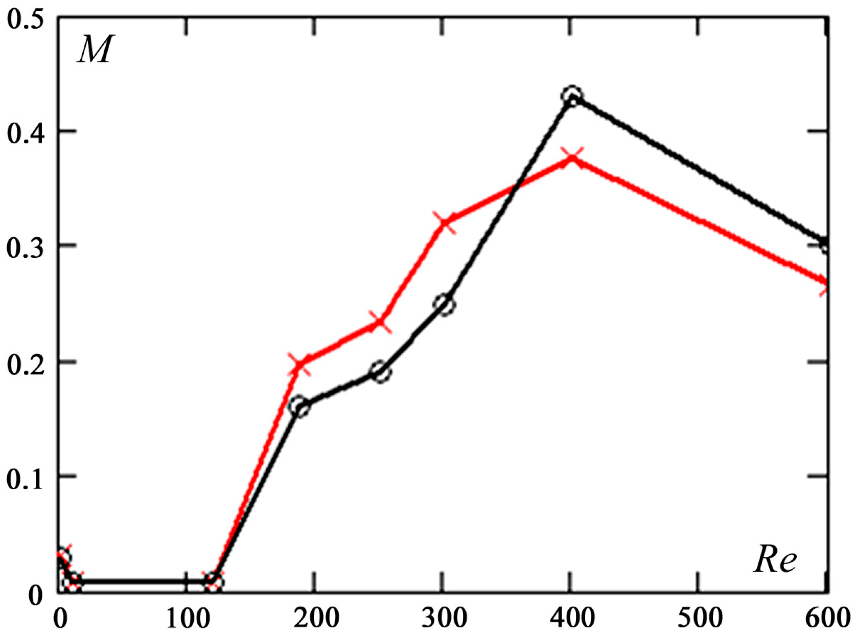
On the other hand, the mixing efficiency behaves differently. At low Reynolds numbers, it is almost the same in both mixers (see
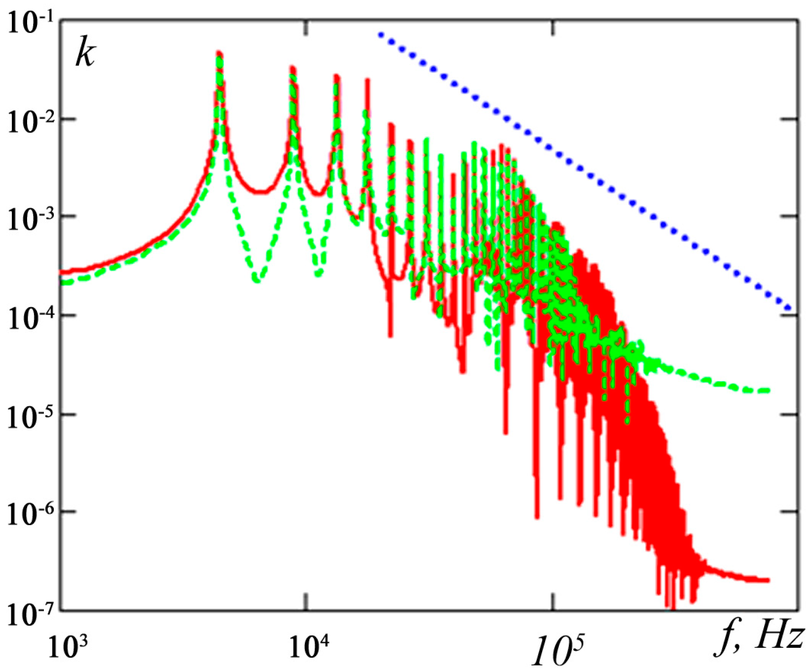
Figure 21). However, with increasing Reynolds number to Re ~ 350, the mixing efficiency in the smooth channel is higher than that in the rough channel. At high Reynolds numbers, the efficiency of the rough channel becomes higher. This is due to the fact that turbulence develops earlier in the rough channel than in the smooth channel. Spectra of the kinetic energy
E of velocity fluctuations in the channels are compared in
Figure 22, where the solid curve corresponds to the rough channel and the dashed curve to the smooth channel.
Figure 20.
Pressure drop in the channel versus the Reynolds number.
Figure 20.
Pressure drop in the channel versus the Reynolds number.
Figure 21.
Mixing efficiency versus the Reynolds number.
Figure 21.
Mixing efficiency versus the Reynolds number.
Figure 22.
Kinetic energy spectrum of velocity fluctuations at Re = 300.
Figure 22.
Kinetic energy spectrum of velocity fluctuations at Re = 300.
5. Experimental Study of Flow Regimes in T-Type Micromixers
Experimental studies of microflows involve obvious difficulties. There are two methods widely used in these studies: micro-particle image velocimetry (micro-PIV) and laser-induced fluorescence (micro-LIF). In the micro-PIV method [
37], successive tracer images are recorded at regular time intervals with subsequent cross-correlation processing of the images. Instantaneous and average velocity fields in a microfluidic device can be calculated knowing the time between the light pulses and the displacement of the tracer particles.
The micro-LIF method [
38] involves measuring temperature and concentration fields with a micron resolution and is based on the fact that the fluorescence intensity is proportional to the concentration of the fluorescent dye and decreases with increasing temperature. In micro-LIF measurements, a fluorophore is added to the flow studied, and the flow is exposed to excitation light. Because the fluorescence intensity is proportional to the dye concentration (if it is low), instantaneous concentration fields can be reconstructed from recorded fluorescence patterns. Below, we describe the experiments performed in [
23,
39].
The imaging system consisted of a Carl Zeiss AxioObserver.Z1 inverted epifluorescence microscope with lenses of 20×/NA (numerical aperture) = 0.3 and 5×/NA = 0.12 for micro-PIV and micro-LIF experiments, respectively. Illumination and image recording by a digital camera were conducted using a POLIS measuring complex, which consists of the following main elements: (1) a double-pulse Nd: YAG laser with a pulse energy of 50 μJ, a wavelength of 532 nm and a pulse repetition rate of 8 Hz, which illuminated the flow through the microscope objective; (2) a liquid optical fiber for coupling the laser radiation into the microscope and a unit for coupling the fiber to the optical system of the microscope; (3) a mercury lamp for illuminating the microchannel in micro-LIF experiments; (4) a cross-correlation digital camera for image recording with a resolution of 2048 × 2048 pixels; (5) a personal computer for data processing; and (6) a programmed processor for synchronizing the operation of the system. The ActualFlow software was used to control the experiment and process the data.
The experiments were carried out in the range of Reynolds numbers from 10 to 300. Fluid flow was controlled by a syringe infusion pump with variable flow rate. The fluid flow was seeded with Duke Scientific fluorescent tracer particles consisting of a melamine resin labeled with the fluorescent dye rhodamine B. The particle density was 1.05 g/cm3; the mean particle diameter was 2 μm, and the standard deviation 0.04 μm. A beam-splitting cube consisting of a diachronic mirror and two filters for excitation and detection of rhodamine B was used to record the light emitted from the particles and to suppress the light reflected from the channel.
A mixer made by MicroLiquid (Arrasate-Mondragón, Spain) was used in the experiments. The cross-sectional dimensions of the inlet and mixing channels of the micromixer were 200 μm × 200 μm and 200 μm × 400 μm, respectively. The length of the inlet and mixing channels was 5 mm. The working fluid was distilled water.
Micro-PIV measurements were carried out in three regions of the T-mixer, so that the velocity field was calculated at distances not exceeding seven calibers from the mixing channel entrance. The measurements were performed in the central plane of the channel at Reynolds numbers from 10 to 300 with an increment of 30. Since, in micro-PIV measurements, the entire depth of the microchannel is illuminated, the thickness of the section where velocity is measured depends on the depth of field of the lens. In this experiment, it was 34 μm.
Figure 23 shows normalized velocity profiles in the central section of the mixing channel at a distance
y = 2.5 calibers from the mixing channel entrance. The profiles were normalized by the velocity
UQ determined by the flow rate
Q at the inlet:
UQ =
Q/ρ
S. Analysis shows that at Reynolds numbers higher than 150, the velocity profile in the channel changes and kinks occur (see
Figure 7). This is due to the formation of an S-shaped structure; a systematic description of this regime is given in the previous section.
Figure 23.
Normalized velocity profiles in the central section of the mixing channel.
Figure 23.
Normalized velocity profiles in the central section of the mixing channel.
In order to correctly interpret the data of micro-LIF measurements and compare them with simulation results, it is necessary to estimate the spatial resolution of the method. In this work, as shown in [
23,
39], the average diameter of spatial averaging was 55 μm. Comparison of the concentration fields obtained by numerical simulation and experiment was performed after spatial averaging over the depth of the T-mixer. This comparison is shown in
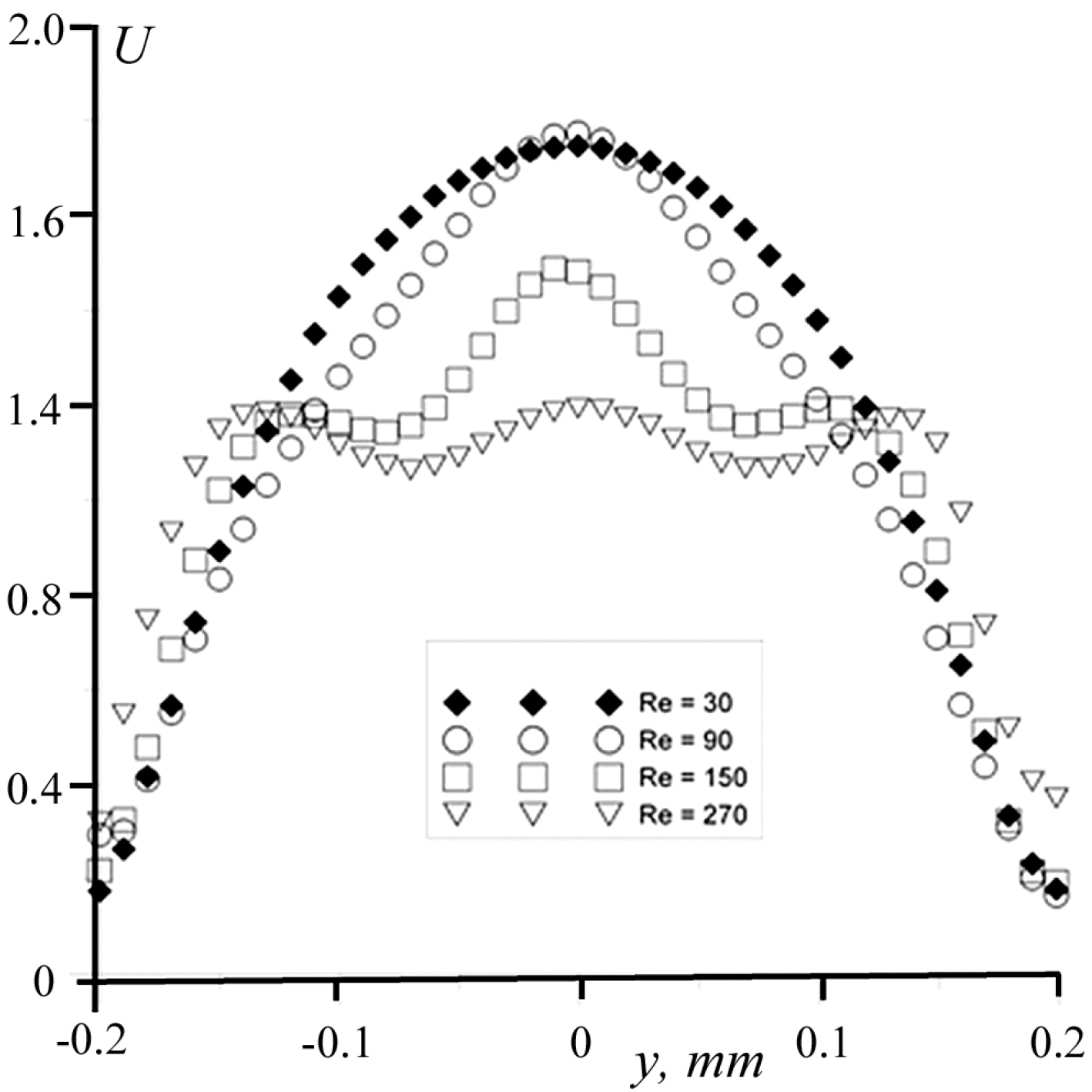
Figure 24. The profiles were obtained in the central section at a distance of 2.5 calibers from the mixing channel entrance. Here, the data points connected by lines are experimental data, and the solid line without data points is the result of numerical simulation. Circles correspond to Reynolds number Re = 30, crosses to Re = 120 and squares to Re = 150. In all cases, the experimental data agree fairly well with the simulation results, but at the maximum Reynolds numbers, the resolution of the interpretation of the experimental data (which is defined by the correlation depth) is not sufficient to adequately describe the complex behavior of the velocity profile involving the formation of S-shaped structures. Numerical simulation turns out to be more accurate.
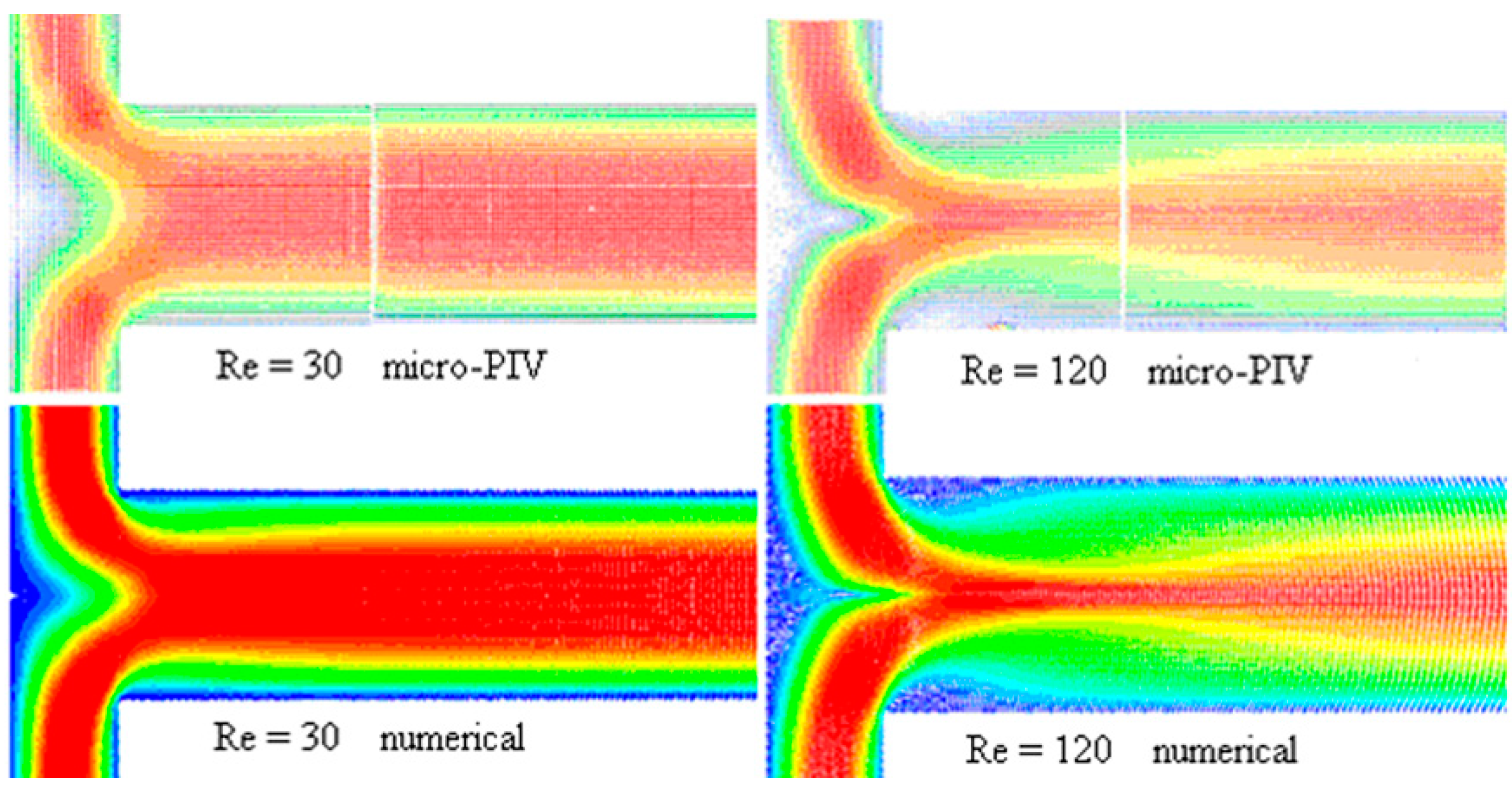
A qualitative comparison of numerical and experimental results is presented in
Figure 25 and
Figure 26, which show velocity isolines at the inlet of the mixer (
Figure 25) and dye concentration isolines in the mixing channel (
Figure 26) for several Reynolds numbers. These data are in fair agreement with each other.
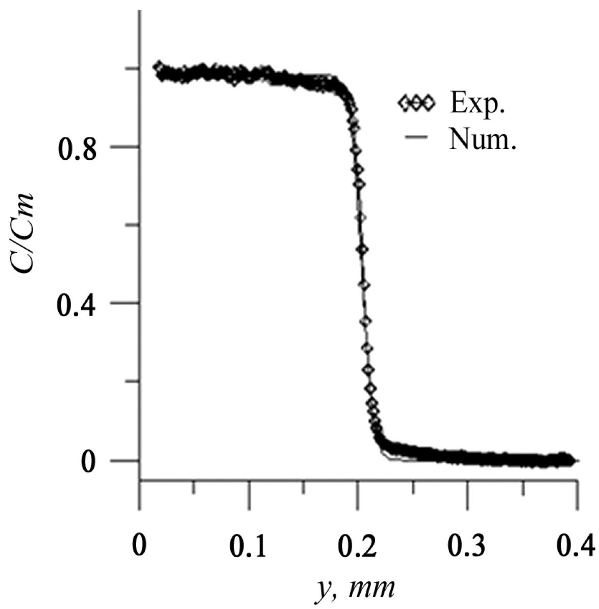
The calculated dye concentration profiles are generally highly consistent with the experimental ones (see
Figure 27). Here, the Reynolds number was Re = 30.
Figure 24.
Velocity profiles in the central longitudinal section of the mixing channel. Circles correspond to Reynolds number Re = 30, crosses to Re = 120 and squares to Re = 150.
Figure 24.
Velocity profiles in the central longitudinal section of the mixing channel. Circles correspond to Reynolds number Re = 30, crosses to Re = 120 and squares to Re = 150.
Figure 25.
Averaged experimental and calculated velocity fields in the central longitudinal section of the mixer.
Figure 25.
Averaged experimental and calculated velocity fields in the central longitudinal section of the mixer.
Figure 26.
Averaged experimental and calculated concentration fields in the central longitudinal section of the mixer.
Figure 26.
Averaged experimental and calculated concentration fields in the central longitudinal section of the mixer.
Figure 27.
Comparison of the experimental and calculated concentration C profiles in the central longitudinal section of the mixer.
Figure 27.
Comparison of the experimental and calculated concentration C profiles in the central longitudinal section of the mixer.
6. Active Mixing Method
In this section, we give an example of an active mixer with variation in the fluid flow rate in the inlet channels. A series of calculations were performed in which the flow rate ratio
Q1/
Q2 in the upper and lower inlets of the mixer channel was varied from 0.25 to 1. Three different flow regimes (see
Section 5) were considered: a symmetric steady regime, Re = 120, an asymmetric steady regime, Re = 186, and an unsteady periodic regime, Re = 250.
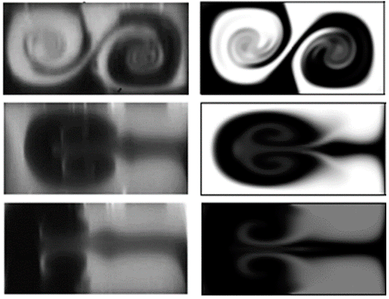
Figure 28 shows a qualitative comparison of the numerical simulation data and experimental results [
11] obtained for the mixing regime in the microchannel cross-section at a Reynolds number Re = 186 and various flow rate ratios.
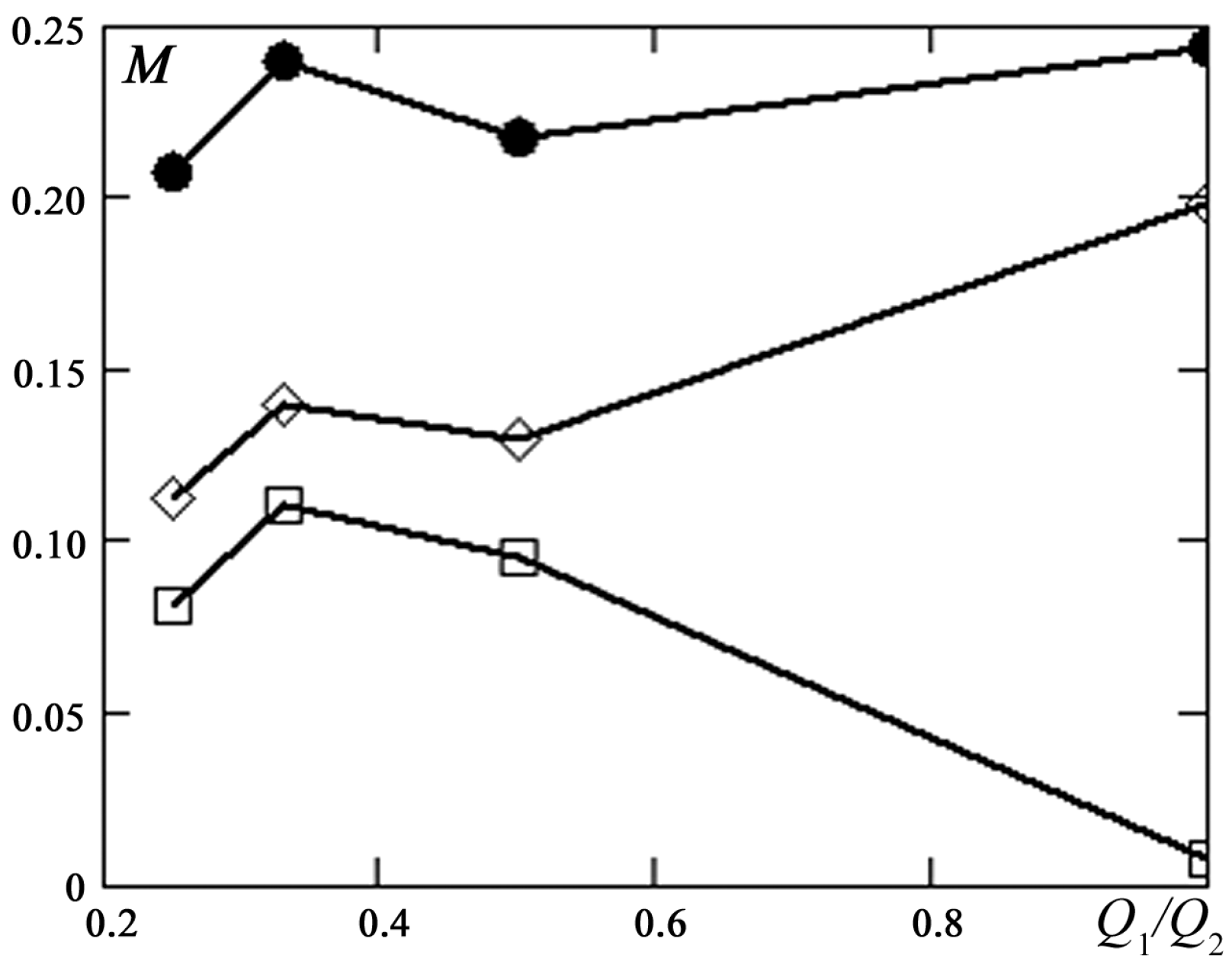
Curves of the mixing efficiency
versus asymmetry in the inlet flow rate for various Reynolds numbers are presented in
Figure 29. The behavior of the curves greatly depends on the Reynolds number. For a Reynolds number Re = 120 (lower curve), asymmetry in the inlet conditions provides a significant (factor of 15) enhancement of the mixing. Maximum mixing efficiency is observed at
Q1/
Q2 = 1/3. At Reynolds numbers greater than 150, at which an S-shaped vortex structure is formed in the channel, the presence of artificially asymmetry leads to the destruction of this structure and worsening of the mixing performance.
Figure 28.
Qualitative comparison of the mixing regime obtained in experiment [
11] (
left) with calculated data (
right) at a Reynolds number Re = 186 and various flow rate ratios: (
top)
Q1/
Q2 = 1, (
middle)
Q1/
Q2 = 1/2 and (
bottom)
Q1/
Q2 = 1/3.
Figure 28.
Qualitative comparison of the mixing regime obtained in experiment [
11] (
left) with calculated data (
right) at a Reynolds number Re = 186 and various flow rate ratios: (
top)
Q1/
Q2 = 1, (
middle)
Q1/
Q2 = 1/2 and (
bottom)
Q1/
Q2 = 1/3.
Figure 29.
Mixing efficiency versus flow rate ratio at the inlets of the mixer for various Reynolds numbers. The lower curve corresponds to Re = 120, the middle curve to Re = 186 and the lower curve to Re = 250.
Figure 29.
Mixing efficiency versus flow rate ratio at the inlets of the mixer for various Reynolds numbers. The lower curve corresponds to Re = 120, the middle curve to Re = 186 and the lower curve to Re = 250.
One of the simplest methods of active mixing in Y- and T-type mixers is to periodically change the flow rate at one of the inlets. A study [
25] was performed with variation in the velocity
UQ, determined by the flow rate
Q at the upper inlet of a T-type micromixer:
UQ = Q/ρ
S, where ρ is the liquid density and
S is the cross-sectional area of the microchannel. The velocity was given by:
The parameters in Expression (11) are generally determined by the characteristic dimensions of the channel where mixing occurs and flow characteristics (Reynolds and Péclet numbers). It is clear that if the characteristic mixing time is much shorter than the period of change in the flow rate τm << (2πf)−1 = Tf, the mixing efficiency will change little compared to steady mixing. Therefore, the most preferred situation is one in which τm >> Tf. On the other hand, the period of change in the flow rate should be shorter than the characteristic flow time Tf < τL. Of course, producing high-frequency fluctuations in microchannels is technologically difficult. Therefore, the most reasonable situation is one in which τm ≥ (2πf)−1. The optimal fluctuation amplitude can be easily estimated by considering the volume of mixing fluid for the period Tf.
These qualitative considerations are confirmed by direct calculations. As an example, we consider mixing of two fluids in a T-type micromixer. The mixer is 200 μm wide, 120 μm high and 2000 μm long;
U0 = 10
−3 m/s. The fluid has a viscosity coefficient μ = 6.67 × 10
−4 Pa·s and a diffusion coefficient
D = 7 × 10
−11 m
2/s, which corresponds to numbers Re = 0.3 and
Pe = 3000. For these parameters, τ
m ~ 560 s and τ
L ~ 2 s. Therefore, the optimal frequency should satisfy the conditions
Tf < 2 s and τ
m ≥
Tf. The corresponding frequency is determined by the following condition:
fop > 0.08 Hz. This estimate gives the following frequency:
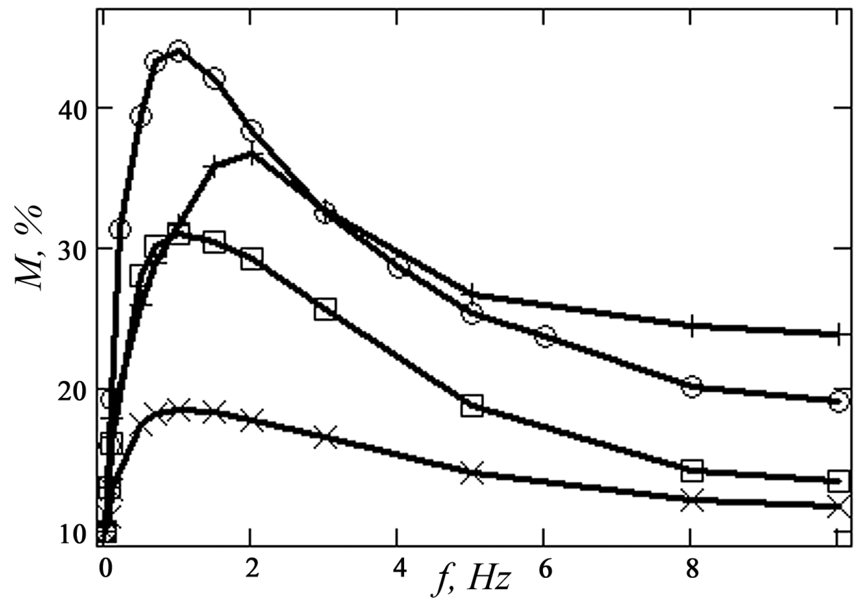
fop ~ 1 Hz. Curves of the mixing efficiency in this mixer
versus frequency
f and amplitude V are presented in
Figure 30. Indeed, optimal mixing is obtained at a frequency of about 1 Hz.
Figure 30.
Mixing efficiency in the T-mixer versus frequency f and amplitude V of fluctuations of the flow rate at one of the inlets. × represents the amplitude V = 1 mm/s, □ to V = 5 mm/s, ○ to V = 10 mm/s.
Figure 30.
Mixing efficiency in the T-mixer versus frequency f and amplitude V of fluctuations of the flow rate at one of the inlets. × represents the amplitude V = 1 mm/s, □ to V = 5 mm/s, ○ to V = 10 mm/s.
7. Conclusions
The data presented in this paper indicate that the simulation of micromixers is an adequate method for obtaining the necessary information on the flow regimes and mixing efficiency. In many cases, modeling can be a substitute for the experiment for studying micromixers. This is primarily due to the fact that modeling is a more economical method of obtaining information. In addition, experimental studies of microflows usually provide information only about integral flow characteristics (flow rate, pressure drop, etc.). However, the experimental information is very important of course in all cases.
In practice, however, detailed data are often required, which generally can be easily obtained by modeling. At the same time, the modeling studies presented in this paper used a hydrodynamic description of microflows. One should clearly understand the limitations of this approach. This issue is briefly discussed below.
A hydrodynamic description for a one-component fluid is applicable if the state of the system under consideration is described by hydrodynamic variables: density, velocity and temperature (pressure). This is possible if we can distinguish a physically infinitesimal scale on which these variables do not change; furthermore, in the topology of the fluid considered, the corresponding volume is a material point. It can be shown that this scale is of order
![]()
[
40], where
d is the characteristic linear scale of the flow (diameter of a cylindrical channel, the distance between plates in plane Poiseuille flow,
etc.) and σ is the characteristic size of the fluid molecules. Appreciable fluctuations in the number of particles in this volume are observed even in channels with a characteristic size of about 1 μm. Therefore, in the presence of gradients of macroscopic variables in flow, the hydrodynamic description ceases to be valid.
Special problems arise near the channel walls. In gases, the viscosity is related to the momentum transfer by molecules, and therefore, it generates on scales larger than the mean free path of the molecules. In liquids, a short-range order exists on scales of the order of 1 nm and viscosity generates onmesoscales of rl: σ < rl < rh. Thus, the viscous fluid conception only works for scales starting from tens of nanometers. Therefore, fluids in small microchannels may have different viscosity near the wall and in the bulk. In addition, transport processes in microchannels generally cease to be isotropic. For example, the diffusion of molecules along and across a channel may be different.
In the modeling of gas flows, the hydrodynamic method can be used only for Knudsen numbers Kn = l/d ≤ 10−3, where l is the mean free path of the gas molecules. In microchannels, this condition is only satisfied for dense gases.
In dispersed fluids, the situation is much more complicated, since the conditions of applicability of the hydrodynamic description must be satisfied for both the carrier fluid and the pseudo-gas of dispersed particles. Here, as a rule, the state of the fluid cannot be described by uniform hydrodynamic variables. A multifluid description is required in which the state of the carrier fluid and dispersed particles is described by partial hydrodynamic variables. However, the Knudsen number for pseudo-gas particles is typically not small. In this case, a mixed description should be used: the carrier component, a gas or a liquid, is described hydrodynamically, and dispersed particles are described kinetically [
41,
42].
Finally, we have to notice that gas-liquid systems are widely used in practice. However, the frame of this paper did not permit us to discuss this subject.


 , which can be great in gases (here, the wall slip length b is given by the condition v = b(∂v/∂x), where the flow occurs along the X-axis, v is the flow velocity in this direction and the Y-axis is perpendicular to the channel wall the λ-mean free path of the molecules). In macroflows of a liquid under normal conditions, the slip length ranges from a few nanometers to several tens of nanometers. This slip can be neglected. In microflows, however, this slip can be significant. In addition, the slip length in microflows can reach a few hundred nanometers. This is due to a change in the short-range order of the fluid near the surface, possible gas release at the channel walls, etc. The presence of slip leads to a significant decrease in the frictional resistance at the channel walls and, hence, to a reduction in the pressure drop. The slip length can be increased by using various hydrophobic or even ultra-hydrophobic coatings (see, e.g., [26,27]). In this case, the slip length can reach tens of micrometers.


 [36], where R is the radius of curvature of the flow turning. In the channel studied in this work, Dean vortices were observed at Re ≈ 20. If the radius of the flow turning in this microchannel is set equal to R = d/2, this corresponds to a critical Dean number Dn = 28.


 is its average value, and
  ).
).


 [40], where d is the characteristic linear scale of the flow (diameter of a cylindrical channel, the distance between plates in plane Poiseuille flow, etc.) and σ is the characteristic size of the fluid molecules. Appreciable fluctuations in the number of particles in this volume are observed even in channels with a characteristic size of about 1 μm. Therefore, in the presence of gradients of macroscopic variables in flow, the hydrodynamic description ceases to be valid.