3.1. Overview of Our Work
Figure 1 shows an overview of our work. In part “the proposed universal multi-lead QRS detector”, the length of the input ECG signal is designed as being 10 s. Then, the 10 s ECG signal is filtered by a band-pass filter whose lower pass-band frequency and upper pass-band frequency are 1 Hz and 40 Hz, respectively [
12]. Subsequently, a simple scaling operation is conducted on the filtered ECG signal and the output of the QRS detector, corresponding to the downsampling operation and the upsampling operation in
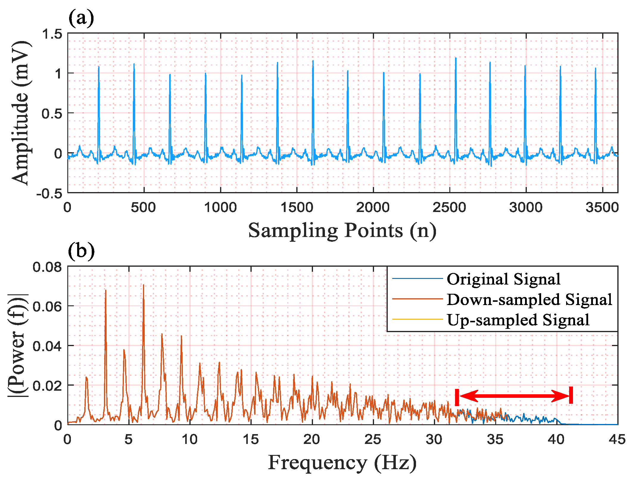
Figure 1. The scaling factor is 0.2. For example, suppose that the length of the ECG signal is 3600 sampling points; after downsampling the ECG signal with the scaling factor of 0.2, the length becomes 720 sampling points. Similarly, the length of the output of the QRS detector is upsampled to 5 times (1/0.2). Finally, in the predicted result, the QRS complexes are predicted with values of 1, and other areas are predicted with values of 0; thereby the QRS complexes are detected. The downsampling operation and the upsampling operation are quite important for our QRS detector for the following two reasons:
- (1)
These two operations can largely shorten the length of the input signal, thereby decreasing the computational load.
- (2)
These two operations can remove redundant information from the input signal, thereby improving the performance of the QRS detector.
In the “Databases” part, we employed three open-access databases to evaluate the proposed QRS detector. These are the MITBIH Arrhythmia (MITBIHA) database [
13], the China Physiological Signal Challenge 2019 (CPSC2019) database [
14], and the St Petersburg INCART 12-lead Arrhythmia (INCART) database [
15]. The details of these databases are described in the “Database” part of this section.
In the “Inter-patient Experiments” part, we designed five experiments to evaluate our approach and compared our approach with other state-of-the-art ones. These experiments gave a comprehensive evaluation of the proposed QRS detector, including the in following areas:
- (1)
The performance of the QRS detector when it was trained using single-lead signals and tested using single-lead signals.
- (2)
The performance of the QRS detector when it was trained using single-lead signals and tested using 12-lead signals.
- (3)
The performance of the QRS detector when it was trained using 12-lead signals and tested using 12-lead signals.
- (4)
The performance of the QRS detector when it was trained using 12-lead signals and tested using single-lead signals.
- (5)
The performance of the QRS detector when it was trained using 12-lead signals and tested using signals using different lead configurations.
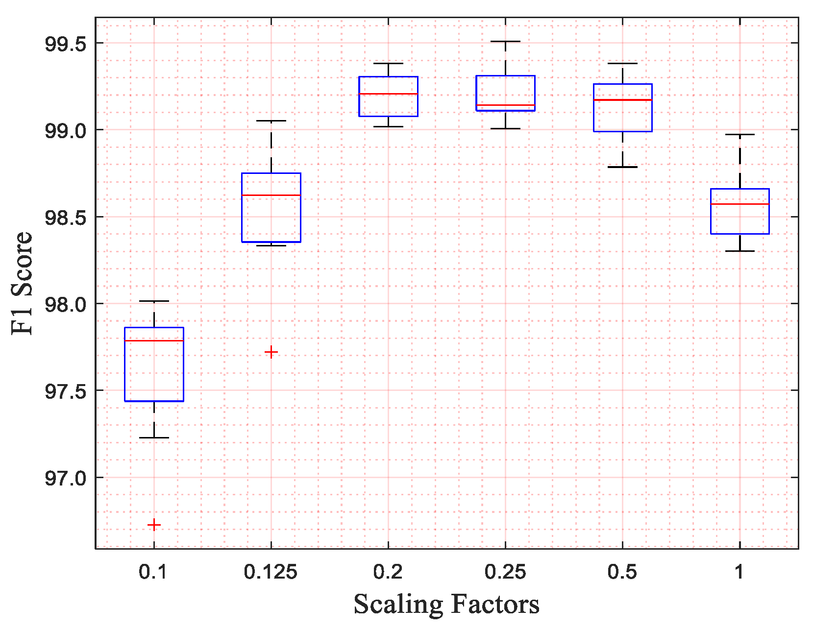
In the “Analysis” part, we additionally designed an experiment to explore the selection of the scaling factor and the reasons for the effectiveness of the scaling operation. In the procedure of exploring suitable scaling factors, we trained and tested our network with different kernel sizes of the input layer and different scaling factors. In this procedure, we only used MITBIHA DS1a and DS1b. The experimental results show that the network performs best when the scaling factor is 0.2. Therefore, we selected the scaling factor of 0.2 as the appropriate one and used it in all experiments. The relevant experimental results are displayed in
Section 4. To explore the underlying reasons as to why the scaling operation can improve network performance, we also conducted a further analysis of the signals from a frequency-domain perspective. The corresponding results are also displayed in
Section 4.
3.2. Leads-Distillation Module
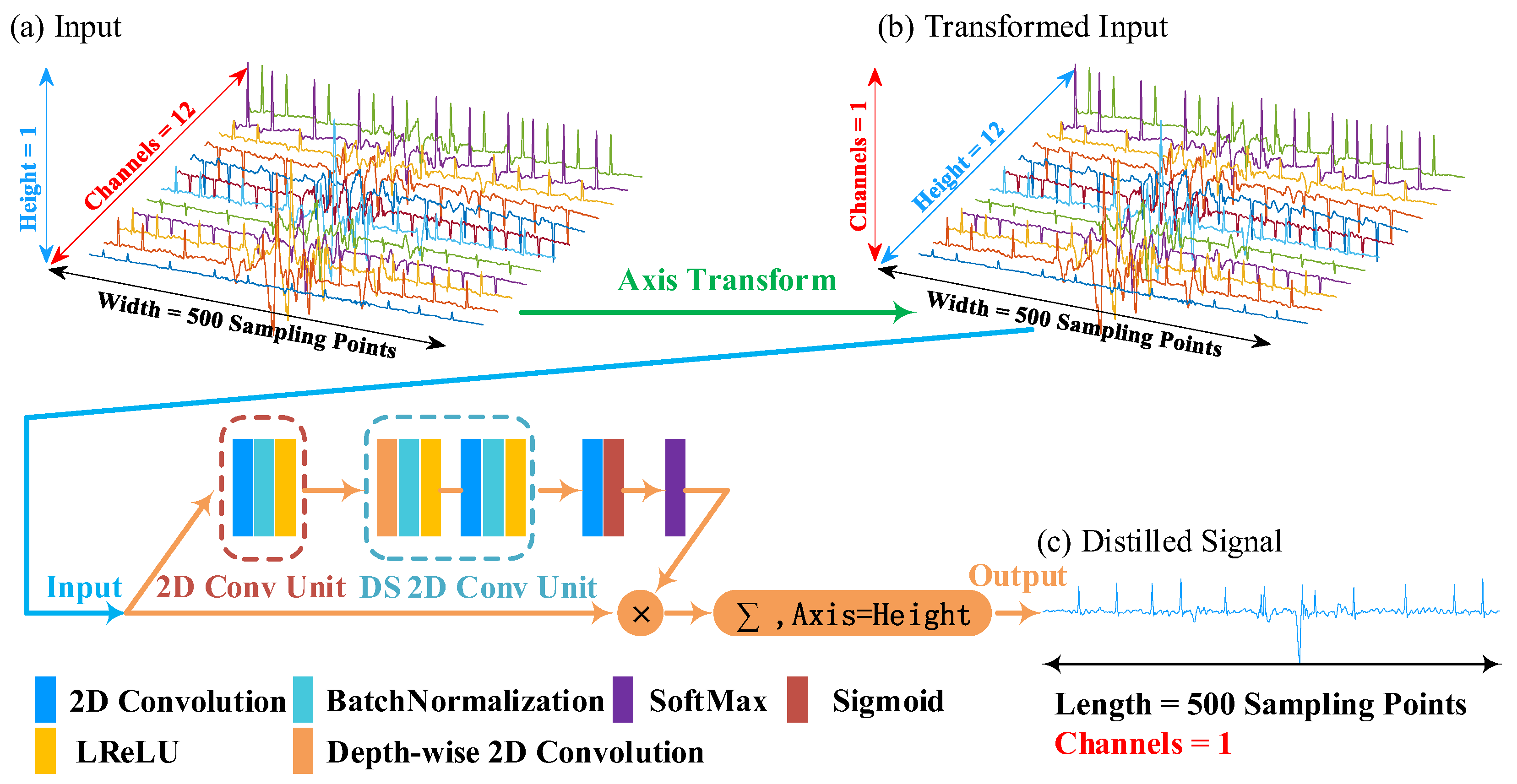
We give an example to illustrate the principle of the leads-distillation module (LDM), as shown in
Figure 2. In this example, we employ a 12-lead signal with a 250 Hz sampling frequency as the input ECG signal. Because the duration of the input signal is 10 s, the length of the input is 2500 sampling points. The input ECG signal is processed through the simple scaling operation, and the length of the input ECG signal becomes 500 sampling points. Because the channel number of a convolution unit is related to that of its input feature map, once the structure of the network has been designed, the channel number of the input cannot be modified [
16,
17]. To realize the function of processing signals with different numbers of leads, we convert the multi-lead signal to a picture that has a large width, a small height, and one channel, as shown in
Figure 2b. We call this procedure the “Axis Transform”, as shown by the green arrow of this figure.
We designed a structure to distill the multi-lead signal into a single-lead one. Firstly, we defined a 2D convolutional unit (2D Conv Unit) to extract features from the transformed input, which consists of three operations: (1) a 2D convolution with n 1 × m kernels and a “same” padding model, (2) a batch normalization (BN) to accelerate gradient propagation [
18], and (3) a leaky rectified linear unit (LReLU) to conduct non-linear functions [
19]. This 2D Conv Unit is denoted as follows:
where
ω and
b are the weights and biases of the 2D convolution.
B(·) denotes the batch normalization operation.
δ(·) denotes the leaky rectified linear unit, which is defined as follows:
where
α is the negative slope and is set to 0.3 in this work.
is a three-dimensional input feature map, and the superscripts H, W, and C denote the height, the width, and the number of channels, respectively. It is defined as follows:
where H, W, and C denote the height, the weight, and channels of the activation map, respectively.
denotes a value in an activation map of channel c.
Suppose that the input is
. The 2D Conv Unit with N convolutions outputs a feature map
, which has N channels and can be denoted as follows:
where
is the feature map of channel i.
Secondly, we employed a depth-wise separable 2D convolution unit (DS 2D Conv Unit) [
20] to further extract features with a small number of parameters and low computational cost. The DS 2D Conv Unit contains two essential components, the depth-wise 2D convolution, and the point-wise 2D convolution. The depth-wise 2D convolution outputs a feature map
, which has N channels and can be denoted as follows:
The remaining layers of the DS 2D Conv Unit are conducted on
and output the feature map
, which is defined as follows:
Thirdly, we utilized a 2D convolution and an activation function “Sigmoid” to squeeze channels from N to 1 and obtained a weight matrix
which has one channel and can be shown as follows:
In this matrix, the width and height are the same as the input . Furthermore, each value of this matrix denotes the weight of each sampling points of .
To obtain the important sampling points among all leads, we conducted the operation “SoftMax” on each column of the matrix
. The procedure can be expressed as follows:
We multiplied the matrix
and the input
to weaken the value of unimportant sampling points of
, which can be denoted as follows:
Finally, we obtained the distilled signal
by summing the values of each column in
, which can be denoted as follows:
where
is the sampling point of the distilled signal.
To gain a deeper understanding of the leads-distillation module (LDM), we visualized the 12-lead ECG signals, the feature maps before and after the SoftMax operation, and the distilled signal, as shown in
Figure 3. In
Figure 3a, there are some noises near the QRS complexes in most leads, and there are even some fake QRS complexes, as shown in the red regions. In stark contrast, the power of these noises is weakened in the distilled signal.
Figure 3b shows the weights of each sampling point of the 12-lead signal, but the important sampling points of each lead are not obvious.
Figure 3c shows the result output from the SoftMax operation, and the important sampling points of each lead are more obvious. In this figure, the weights of some noises, like a QRS complex, are attenuated, as shown in positions indicated by arrows. Furthermore, we list the hyperparameters of the LDM in
Table 1.
3.5. Database
In this work, we employ three open-access databases to evaluate the proposed QRS detector and study our findings, as shown in
Table 3.
The MITBIH Arrhythmia (MITBIHA) database includes 48 half-hour two-channel recordings. These recordings were acquired from the modified limb leads II (ML II) and V (typically V2) with a sampling rate of 360 Hz [
13]. We only used signals acquired from ML II. Following the recommendation of ANSI/AAMI EC57:1998 standards, four recordings that have the pacemaker are not used in this paper; they are recordings 102, 104, 107, and 217. The data distribution of DS1 and DS2 was proposed by De Chazal et al. and is widely used by other researchers [
24]. Moreover, we further divided the dataset “DS1” into two datasets, namely DS1a and DS1b. They were used to investigate our findings and explore the scaling factor for the simple scaling operation.
The China Physiological Signal Challenge 2019 (CPSC2019) database contains 2000 ECG recordings. Each recording has a duration of 10 s and a sampling frequency of 500 Hz [
14]. The ECG signals of this database have only one channel and are noisier than the MITBIHA database [
25].
The St Petersburg INCART 12-lead Arrhythmia (INCART) database has 75 annotated recordings extracted from 32 Holter recordings [
15]. Each recording is 30 min long and has 12 channels. The signals of this database were sampled at 257Hz. The data distribution of DS1 and DS2 was proposed by Víctor Mondelo et al. [
26]. This database was also used to evaluate the performance of our method with different configurations, including six leads, four leads, three leads, two leads, and a single lead. For this purpose, the DS1 was used to train and keep the original number of leads, while the test dataset “DS2” removes irrelevant leads according to the corresponding lead configuration.
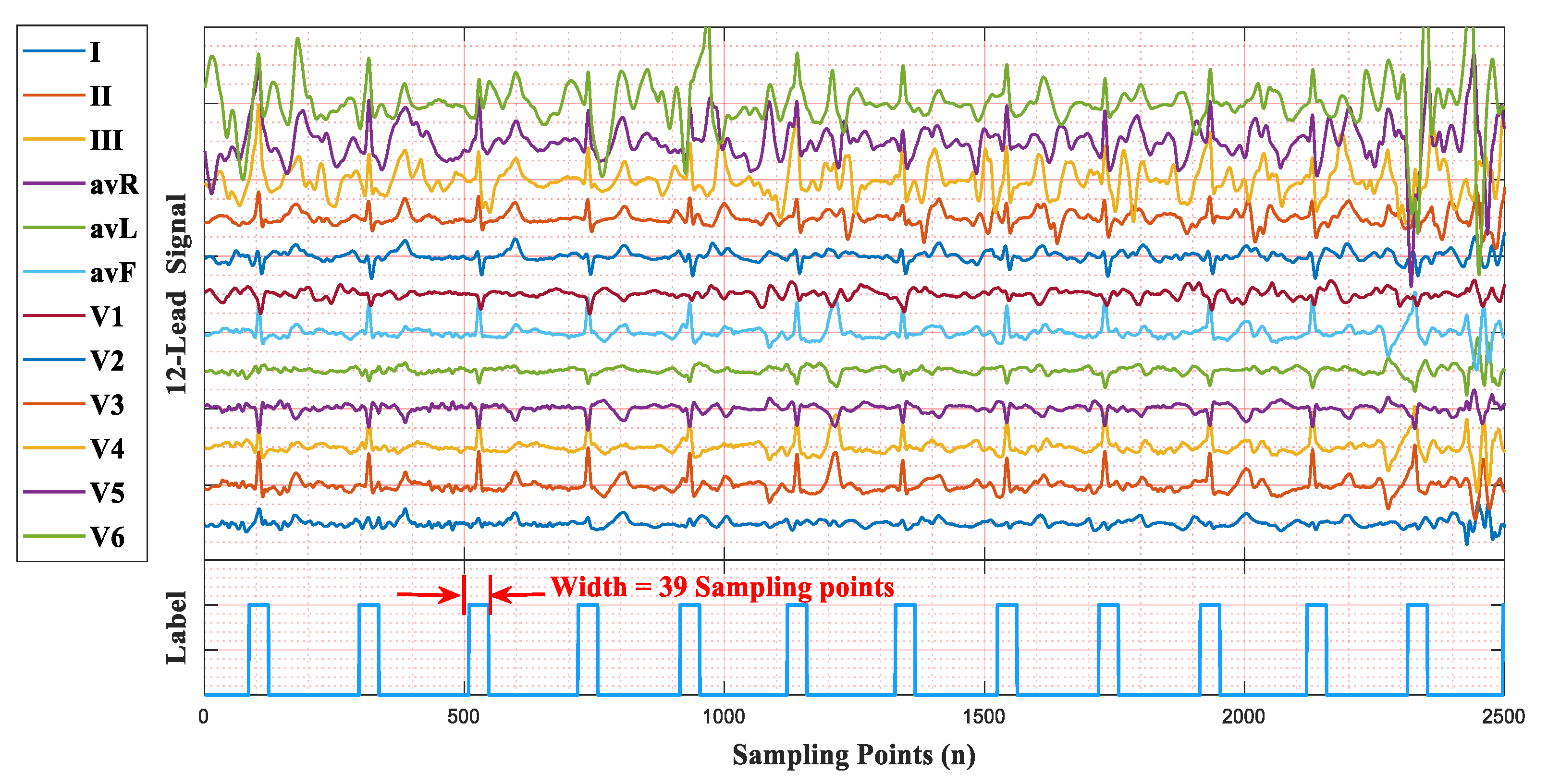
We used a 12-lead ECG signal with a sampling frequency of 257 Hz to illustrate the QRS label, as shown in
Figure 5. The area of a QRS complex is labeled with values of 1, the width is 39 sampling points (19 sampling points before and after an R-peak), and other areas maintain values of 0. The duration of a QRS label is about 150ms, which was selected following the standards of the Association for the Advancement of Medical Instrumentation (AAMI) [
27]. Similarly, for 360 Hz, the width of a QRS label is 55 sampling points, while it is 75 sampling points for 500 Hz.


 and
and 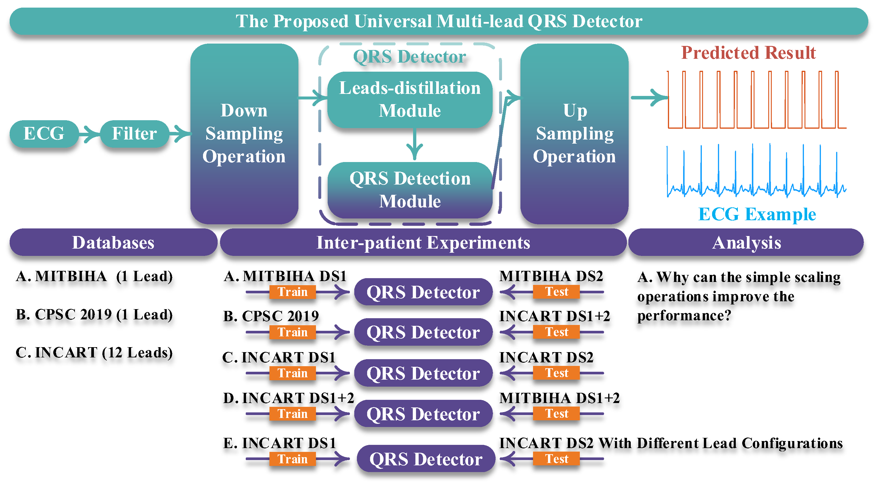


