Author Contributions
Conceptualization, B.L. and P.L.; methodology, P.L.; software, B.L.; validation, P.L., S.L. and P.Y.; formal analysis, P.L.; investigation, B.L. and F.W.; resources, B.L., P.L., and F.W.; data curation, B.L. and L.M.; writing—original draft preparation, B.L.; writing—review and editing, P.L., S.L., L.M. and P.Y; visualisation, B.L.; supervision, P.L. and S.L.; project administration, P.Y.; funding acquisition, P.L. and S.L. All authors have read and agreed to the published version of the manuscript.
Figure 1.
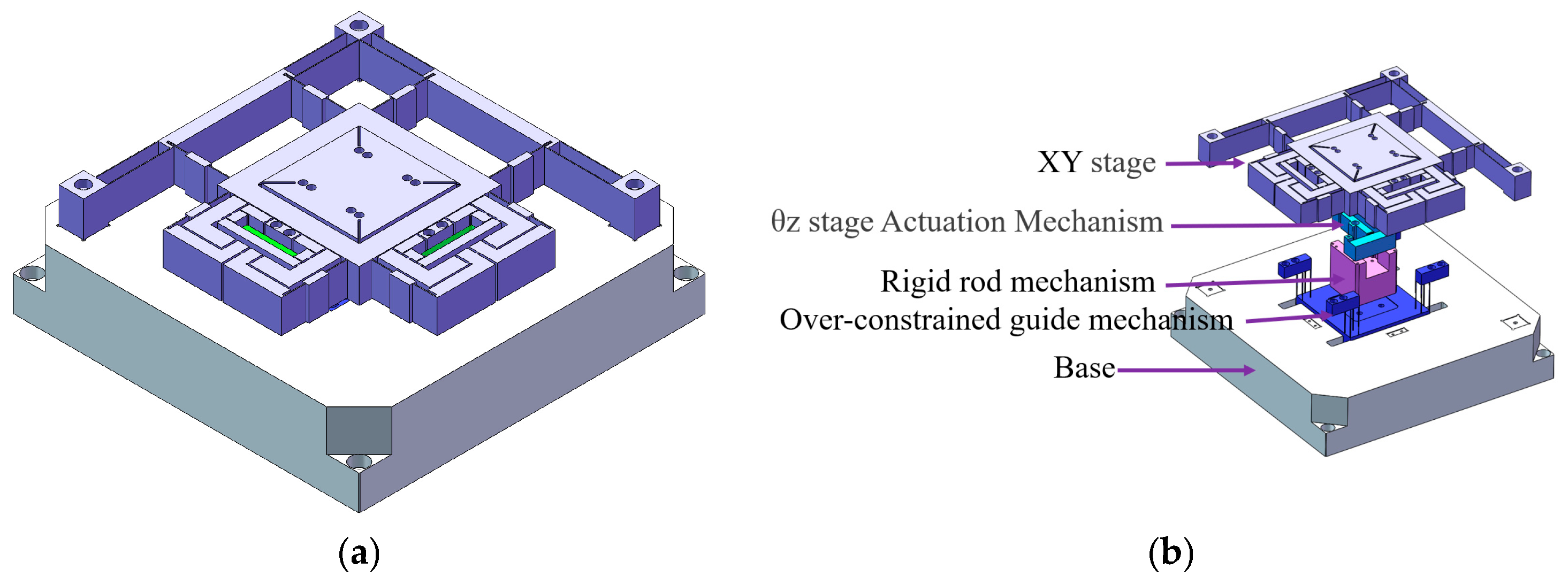
XYθz nano-positioning stage. (a) Isometric view. (b) Exploded diagram and component breakdown of the XYθz nano-positioning stage.
Figure 1.
XYθz nano-positioning stage. (a) Isometric view. (b) Exploded diagram and component breakdown of the XYθz nano-positioning stage.
Figure 2.
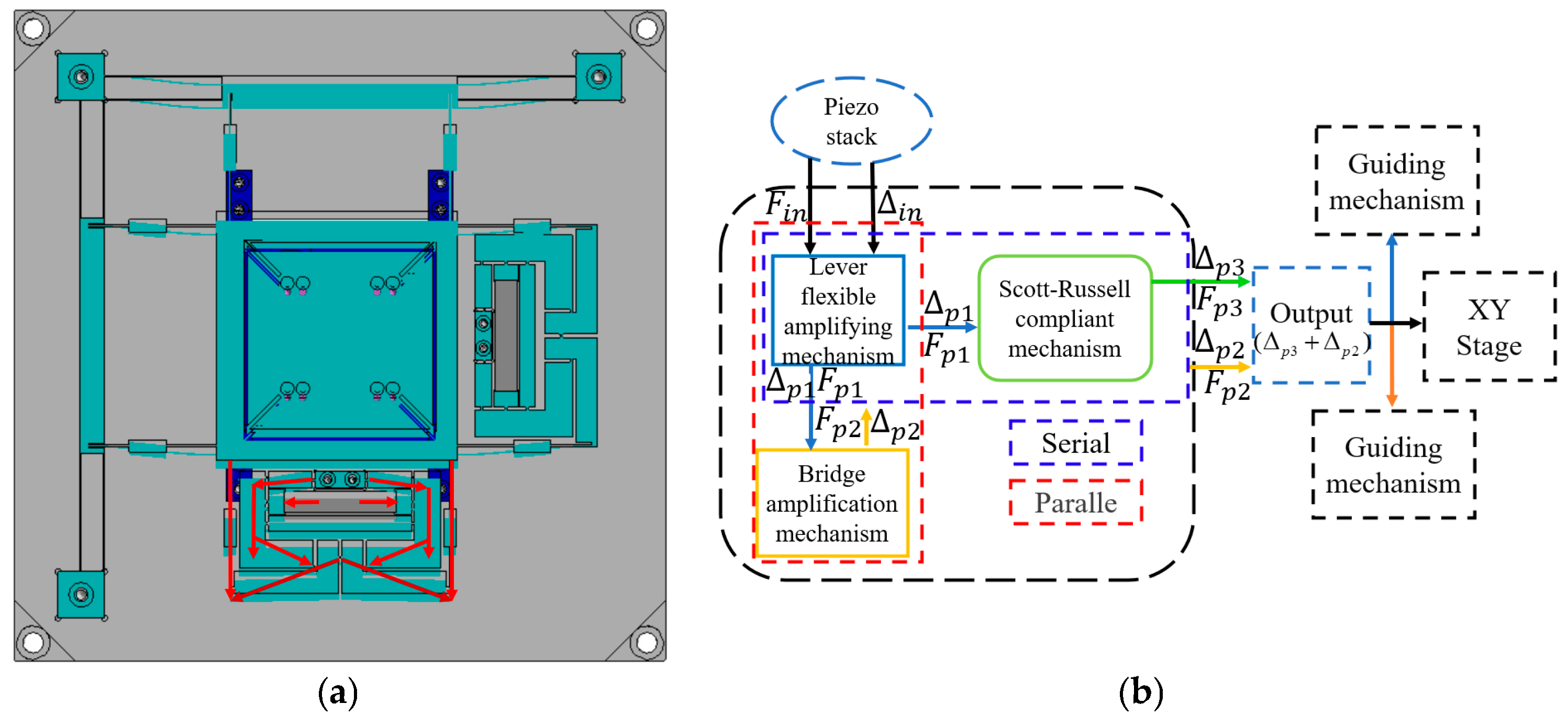
Drive unit of the XYθz nano-positioning stage. (a) XY hybrid amplification mechanism. (b) θz amplification mechanism and over-constrained mechanism.
Figure 2.
Drive unit of the XYθz nano-positioning stage. (a) XY hybrid amplification mechanism. (b) θz amplification mechanism and over-constrained mechanism.
Figure 3.
X/Y directional movement in XYθz nano-positioning stage. (a) Principle of X/Y translational motion. (b) Transmission of X/Y translational motion.
Figure 3.
X/Y directional movement in XYθz nano-positioning stage. (a) Principle of X/Y translational motion. (b) Transmission of X/Y translational motion.
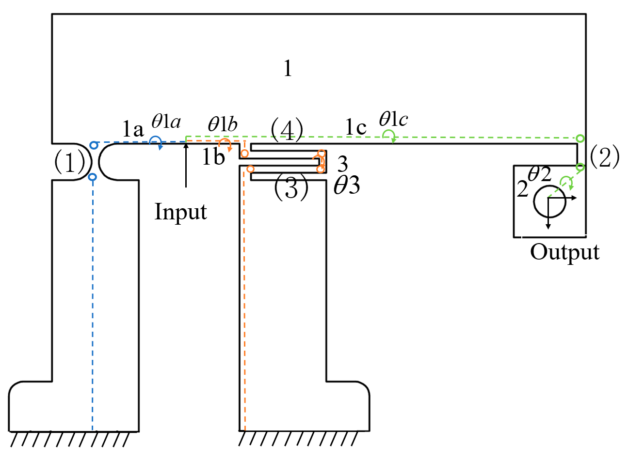
Figure 4.
θz directional movement in XYθz nano-positioning stage. (a) Principle of θz rotational movement. (b) Transmission of the θz rotational movement.
Figure 4.
θz directional movement in XYθz nano-positioning stage. (a) Principle of θz rotational movement. (b) Transmission of the θz rotational movement.
Figure 5.
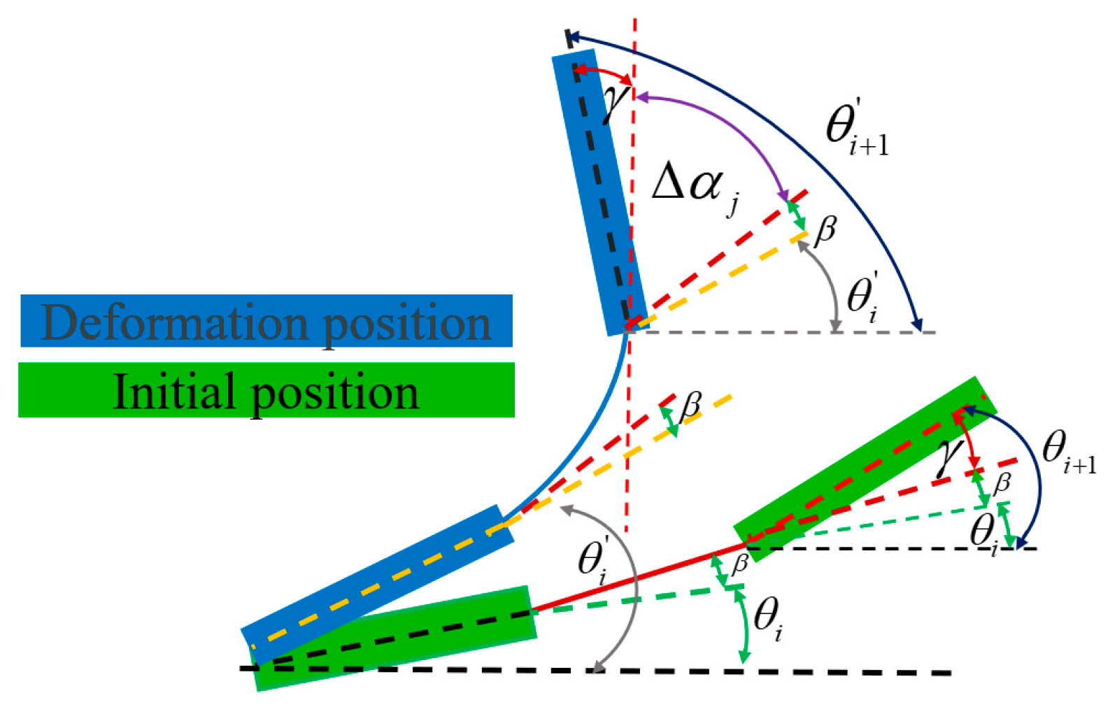
Flexible hinge in the local coordinate system: (a) arc-shaped flexible hinge and (b) straight beam-type flexible hinge.
Figure 5.
Flexible hinge in the local coordinate system: (a) arc-shaped flexible hinge and (b) straight beam-type flexible hinge.
Figure 6.
Angle–displacement relationship.
Figure 6.
Angle–displacement relationship.
Figure 7.
Four motion chains of the XY hybrid amplification mechanism.
Figure 7.
Four motion chains of the XY hybrid amplification mechanism.
Figure 8.
Free-body diagram of XY hybrid amplification mechanism.
Figure 8.
Free-body diagram of XY hybrid amplification mechanism.
Figure 9.
Flexible guide mechanism of the XY stage and hinge division diagram.
Figure 9.
Flexible guide mechanism of the XY stage and hinge division diagram.
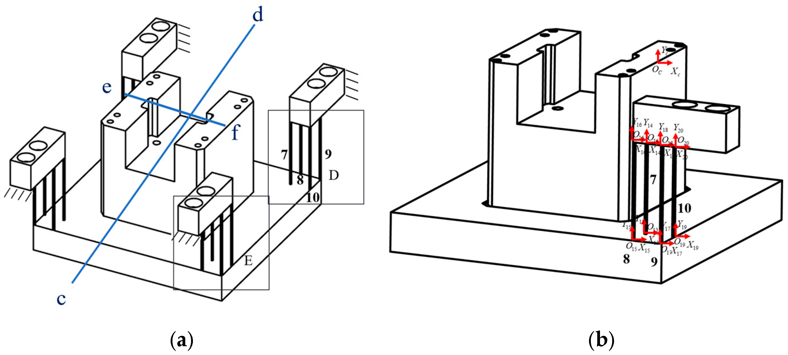
Figure 10.
Size of the guide mechanism of part of the XY stage.
Figure 10.
Size of the guide mechanism of part of the XY stage.
Figure 11.
Modelling system of over-constrained mechanism guide mechanism: (a) hinge division diagram of the over-constrained mechanism guide mechanism; (b) local coordinate map of the hinge of the guide mechanism through the over-constrained mechanism.
Figure 11.
Modelling system of over-constrained mechanism guide mechanism: (a) hinge division diagram of the over-constrained mechanism guide mechanism; (b) local coordinate map of the hinge of the guide mechanism through the over-constrained mechanism.
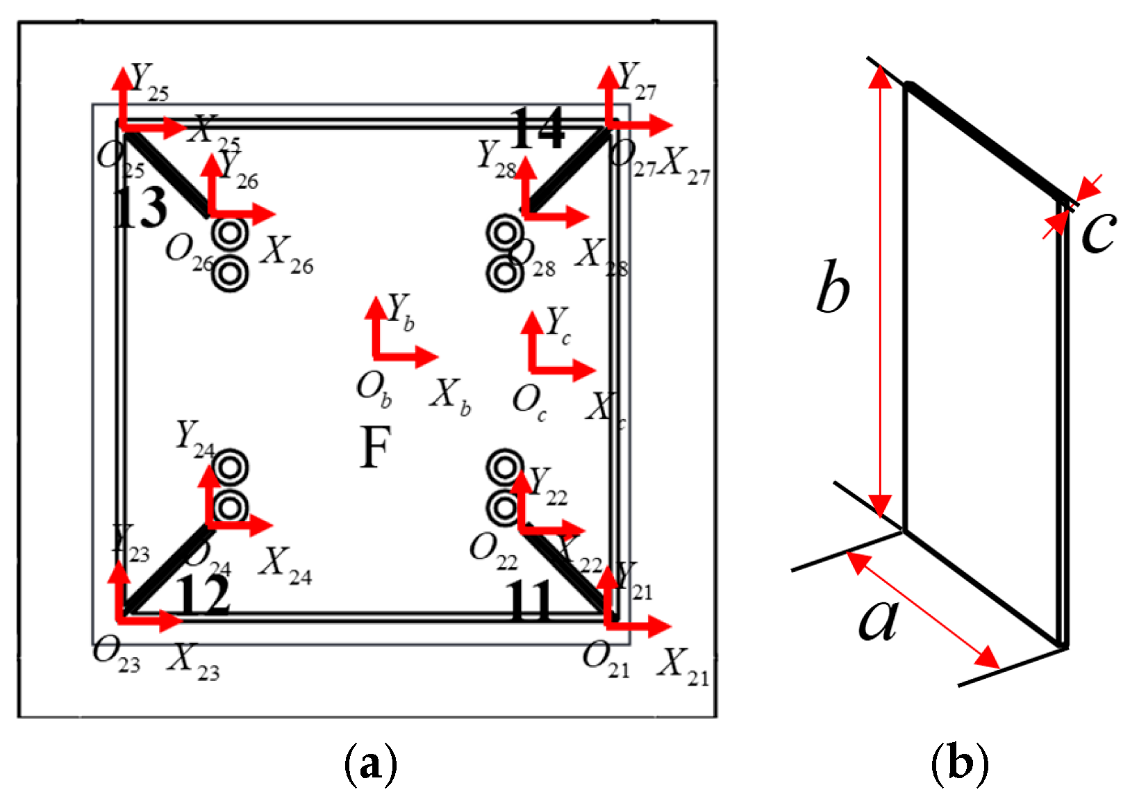
Figure 12.
Size of the guide mechanism of part of the over-constrained mechanism.
Figure 12.
Size of the guide mechanism of part of the over-constrained mechanism.
Figure 13.
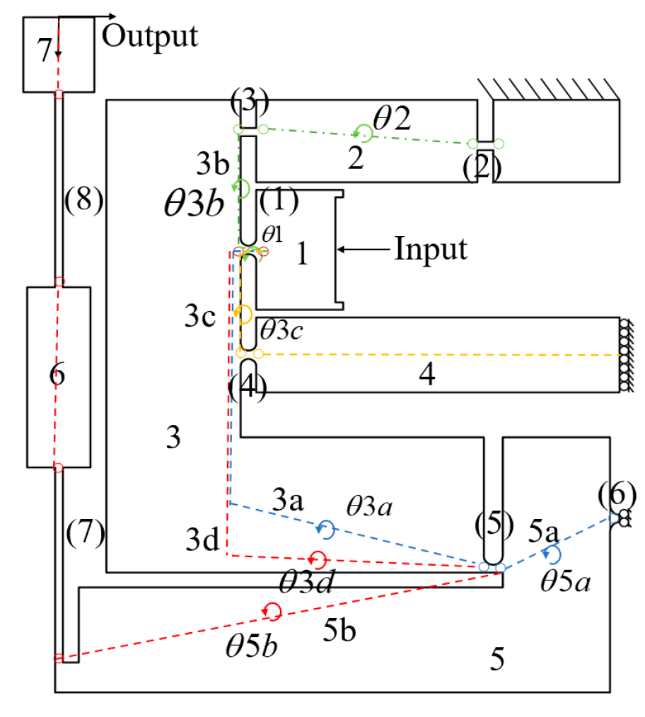
Three motion chains driven by the θz amplification mechanism.
Figure 13.
Three motion chains driven by the θz amplification mechanism.
Figure 14.
Free-body diagram of the θz amplification mechanism.
Figure 14.
Free-body diagram of the θz amplification mechanism.
Figure 15.
(a) Coordinates and distribution map of the hinge of the θz rotating stage. (b) Size of the guide mechanism of part of the θz stage.
Figure 15.
(a) Coordinates and distribution map of the hinge of the θz rotating stage. (b) Size of the guide mechanism of part of the θz stage.
Figure 16.
ANSYS finite element simulation results under 100 N equivalent load: (a) X-axis deformation; (b) Y-axis deformation; and (c) θz-axis deformation.
Figure 16.
ANSYS finite element simulation results under 100 N equivalent load: (a) X-axis deformation; (b) Y-axis deformation; and (c) θz-axis deformation.
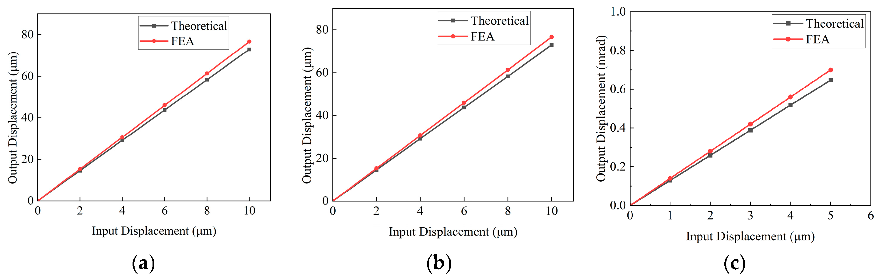
Figure 17.
Relationship between the input and output displacement of the finite element analysis and theoretical results: (a) X-axis; (b) Y-axis; and (c) θz-axis.
Figure 17.
Relationship between the input and output displacement of the finite element analysis and theoretical results: (a) X-axis; (b) Y-axis; and (c) θz-axis.
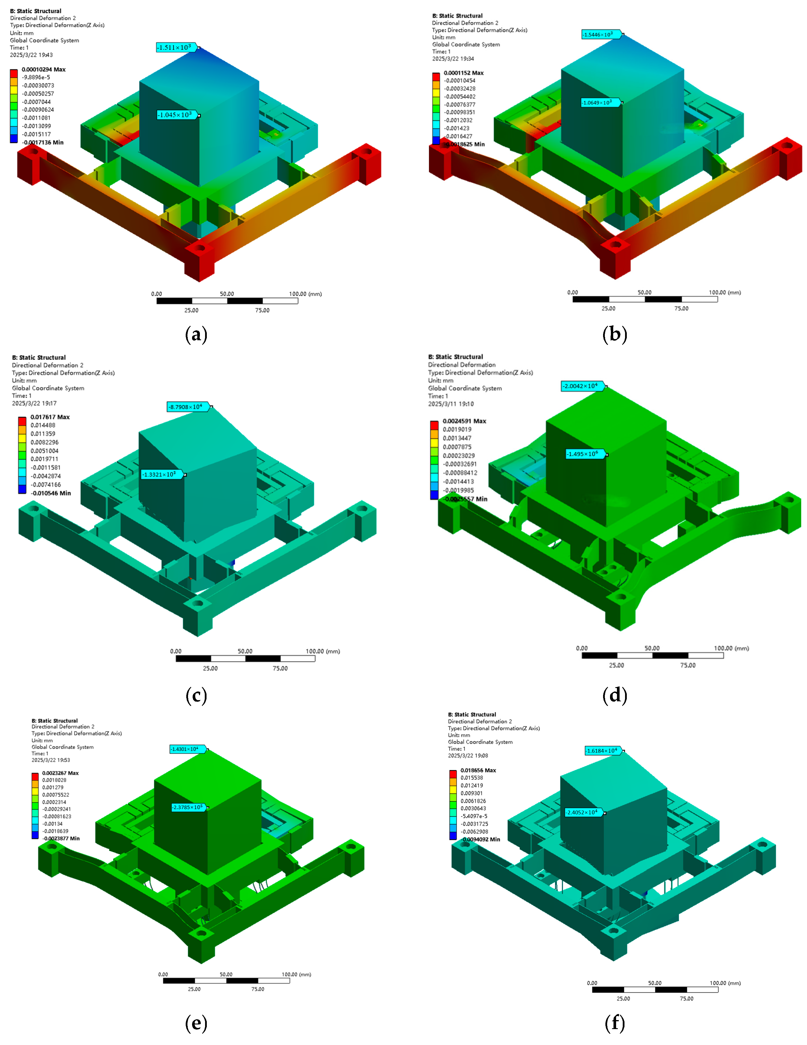
Figure 18.
Flatness of FEA load bearing 4KG with or without over-constrained mechanism: (a) X-axis without over-constrained mechanism, (b) X-axis with over-constrained mechanism (c) Y-axis without over-constrained mechanism, (d) Y- axis with over-constrained mechanism (e) θz-axis without over-constrained mechanism, and (f) θz-axis with over-constrained mechanism.
Figure 19.
FEA (none) over-constrained mechanism with a 4 KG displacement: (a) X-axis without over-constrained mechanism, (b) X-axis with over-constrained mechanism (c) Y-axis without over-constrained mechanism, (d) Y-axis with over-constrained mechanism (e) θz-axis without over-constrained mechanism, and (f) θz-axis with over-constrained mechanism.
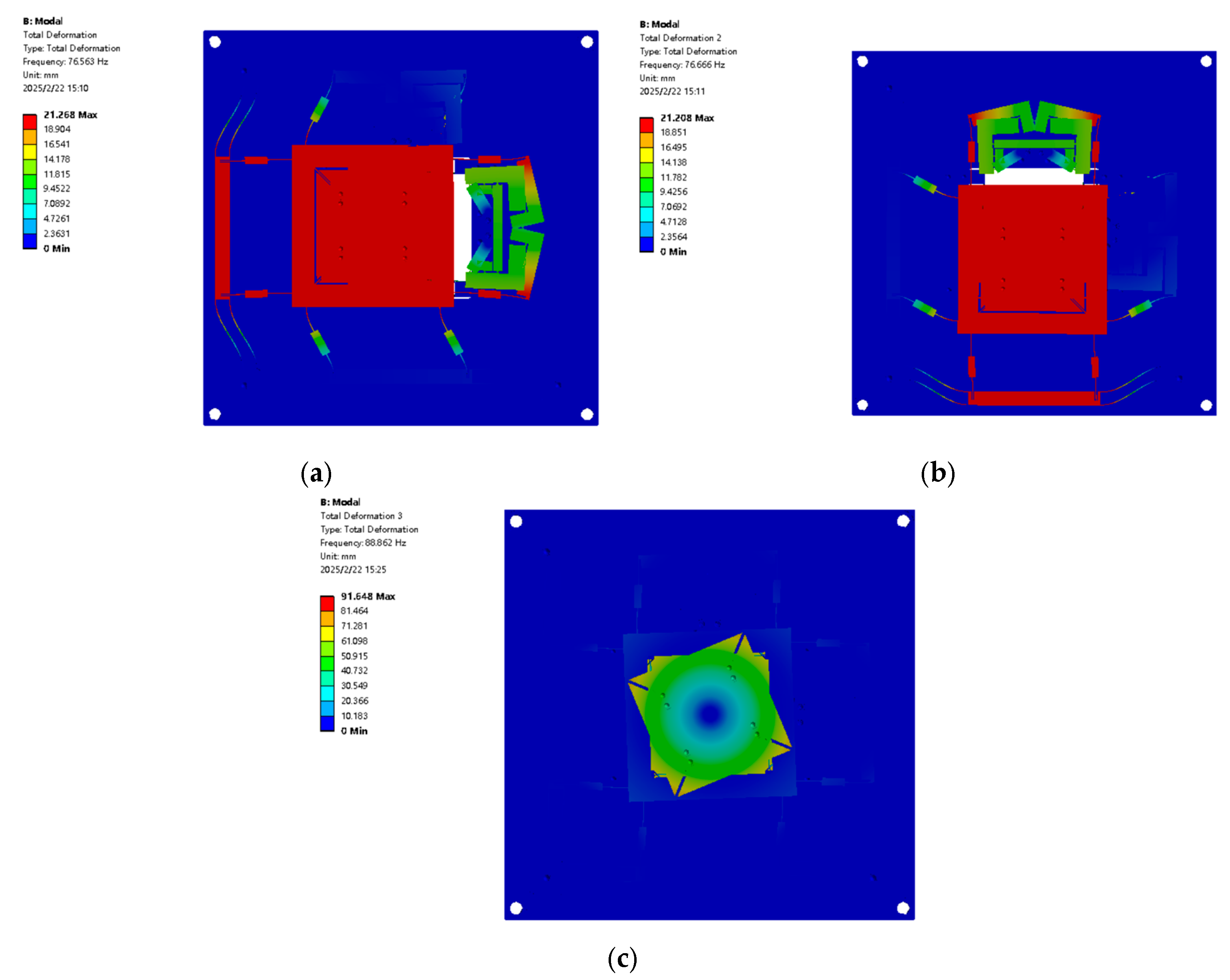
Figure 20.
FEA of the dynamic performance XYθz nano-positioning stage: (a) first-order model; (b) second-order model; and (c) third-order model.
Figure 20.
FEA of the dynamic performance XYθz nano-positioning stage: (a) first-order model; (b) second-order model; and (c) third-order model.
Figure 21.
Experimental device: (a) stroke experiment and (b) load-bearing experiment.
Figure 21.
Experimental device: (a) stroke experiment and (b) load-bearing experiment.
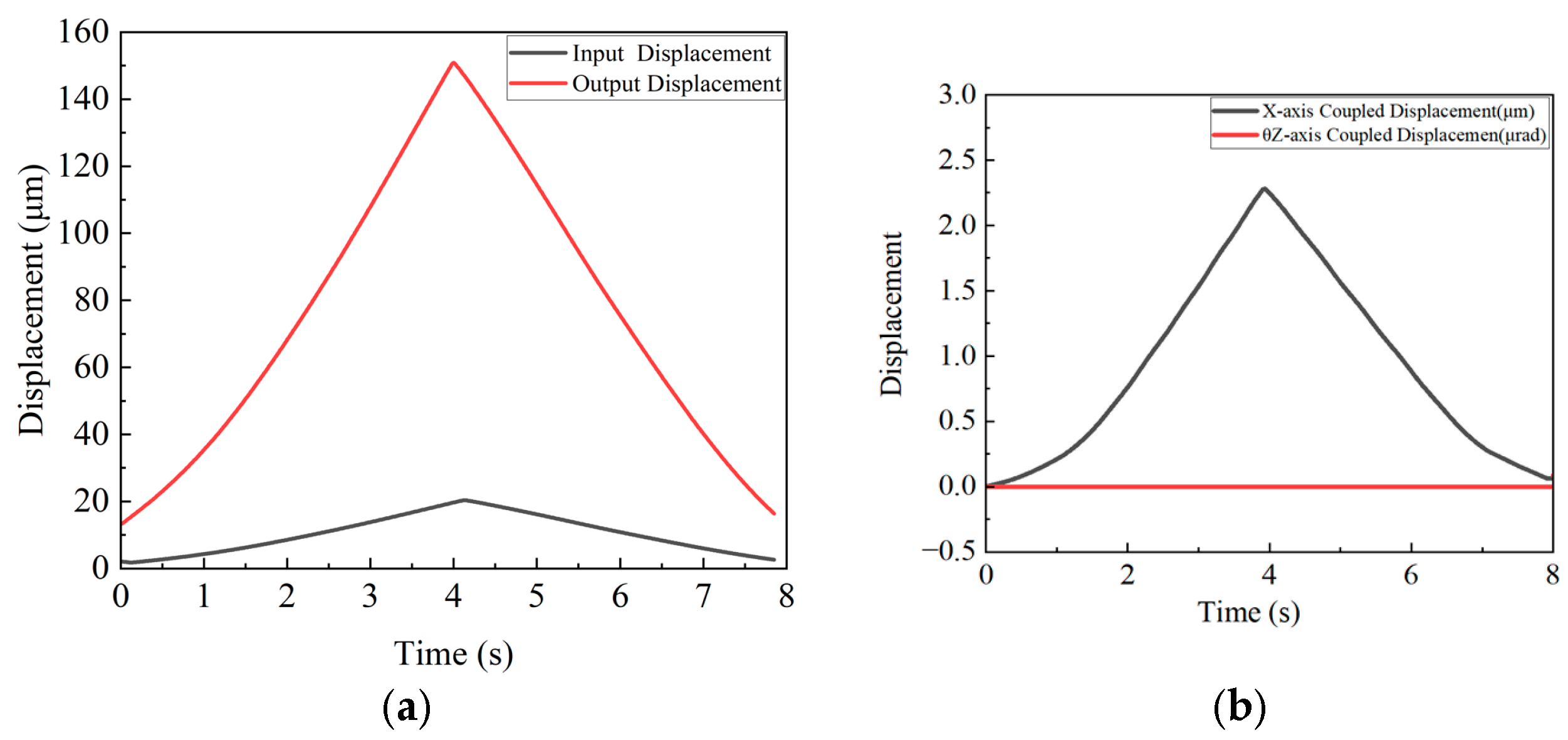
Figure 22.
(a) X-axis input–output displacement curve; (b) X-axis output displacement coupling curve.
Figure 22.
(a) X-axis input–output displacement curve; (b) X-axis output displacement coupling curve.
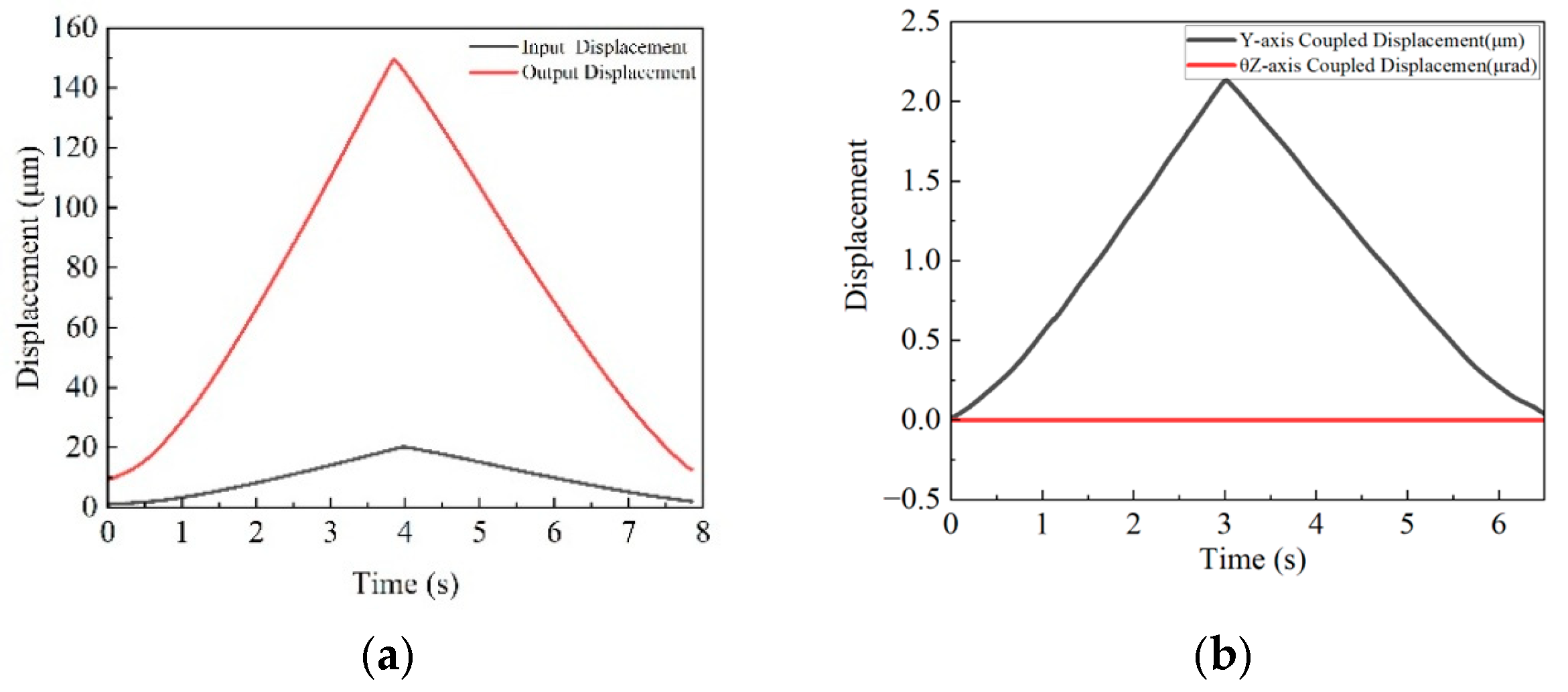
Figure 23.
(a) Y-axis input–output displacement curve; (b) Y-axis output displacement coupling curve.
Figure 23.
(a) Y-axis input–output displacement curve; (b) Y-axis output displacement coupling curve.
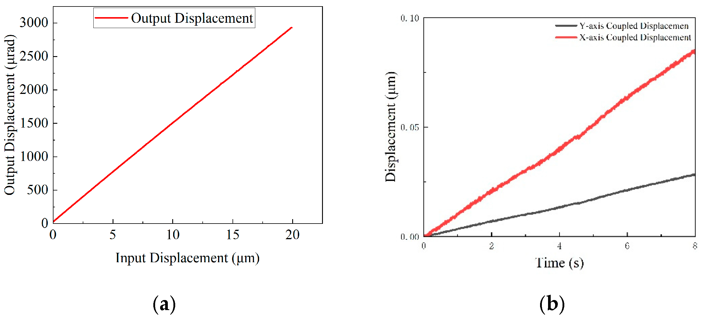
Figure 24.
(a) θz-axis input–output displacement curve; (b) θz-axis output displacement coupling curve.
Figure 24.
(a) θz-axis input–output displacement curve; (b) θz-axis output displacement coupling curve.
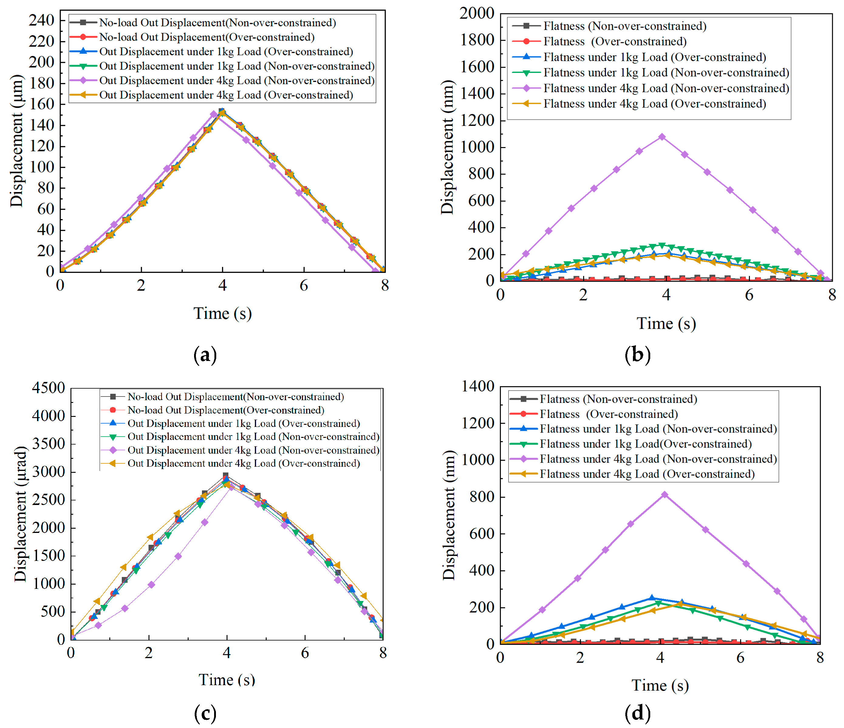
Figure 25.
Influence of axial load on displacement and flatness: (a) X (Y)-axis displacement change; (b) X (Y)-axis flatness change; (c) θz-axis displacement change; and (d) θz-axis flatness change.
Figure 25.
Influence of axial load on displacement and flatness: (a) X (Y)-axis displacement change; (b) X (Y)-axis flatness change; (c) θz-axis displacement change; and (d) θz-axis flatness change.
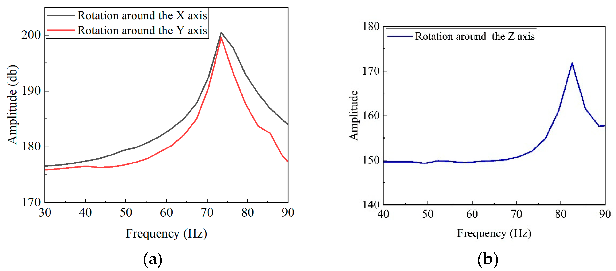
Figure 26.
Frequency response experiment results: (a) XY-axis frequency response curve and (b) θz-axis frequency response curve.
Figure 26.
Frequency response experiment results: (a) XY-axis frequency response curve and (b) θz-axis frequency response curve.
Table 1.
Positioning accuracy of each system.
Table 1.
Positioning accuracy of each system.
| System | Positioning Accuracy |
|---|
| Nanoimprint lithography [5] | 6–40 nm |
| Scanning probe microscopy systems [6] | 20 nm |
| High-precision optical image stabilisation systems [7] | 52 nm |
Table 2.
Specific parameters of the guide mechanism.
Table 2.
Specific parameters of the guide mechanism.
| a (mm) | b (mm) | c (mm) | d (mm) | e (mm) | f (mm) |
|---|
| 13 | 20 | 0.5 | 13 | 38 | 0.45 |
Table 3.
Specific parameters of the over-constrained mechanism.
Table 3.
Specific parameters of the over-constrained mechanism.
| a (mm) | b (mm) | c (mm) | d (mm) |
|---|
| 25 | 0.5 | 0.5 | 7 |
Table 4.
Specific parameters of the guide mechanism of part of the θz stage.
Table 4.
Specific parameters of the guide mechanism of part of the θz stage.
| a (mm) | b (mm) | c (mm) |
|---|
| 16 | 20 | 0.5 |
Table 5.
X/θz amplification mechanism parameter details.
Table 5.
X/θz amplification mechanism parameter details.
| | | 1 | 1a | 1b | 1c | 2 | 3 | 3a | 3b | 3c | 3d | 4 | 5 |
|---|
| X | d (mm) | 5 | - | - | - | 14 | - | 6.19 | 7.85 | 26.7 | 26.7 | 23 | - |
| (°) | 0 | - | - | - | 0 | 0 | - | - | - | - | 90 | 0 |
| θz | d (mm) | - | 6.5 | 3.9 | 30 | 3.3 | 1.5 | - | - | - | - | - | - |
| (°) | 0 | - | - | - | 0 | 90 | - | - | - | | - | |
Table 6.
Comparison of theoretical and FEA results.
Table 6.
Comparison of theoretical and FEA results.
| Direction | Comparative Performance | FEA | Theoretical | Error |
|---|
| X | Amplification | 7.665 | 7.452 | 2.77% |
| Output displacement (μm) | 18.443 | 17.81 | 3.43% |
| Y | Amplification | 7.665 | 7.452 | 2.77% |
| Output displacement (μm) | 18.425 | 17.82 | 3.28% |
| θz | Maximum output displacement (μrad) | 2890 | 2755.9 | 4.64% |
| Output displacement (μrad) | 447.8333 | 438.24 | 2.14% |
Table 7.
Impact of over-constrained mechanism on stage performance in FEA.
Table 7.
Impact of over-constrained mechanism on stage performance in FEA.
| | Displacement | Displacement Deviation | Flatness | Flatness Deviation |
|---|
| X | 158.49 μm | 1.90% | 1.5111 μm | 84.26% |
| X (Over-constrained) | 155.47 μm | 0.2378 μm |
| Y | 158.57 μm | 1.92% | 1.5446 μm | 87.02% |
| Y (Over-constrained) | 155.52 μm | 0.2004 μm |
| θz | 3031.7667 μrad | 4.16% | 1.3321 μm | 81.94% |
| θz (Over-constrained) | 2905.6 μrad | 0.2405 μm |
Table 8.
Modal frequencies of X Yθz nano-positioning stage.
Table 8.
Modal frequencies of X Yθz nano-positioning stage.
| Order | Modal Frequency (Hz) |
|---|
| First-order model | 76.563 |
| Second-order model | 76.666 |
| Third-order model | 88.86 |
Table 9.
Comparison of experimental and FEA results for 4 kg load-bearing stage.
Table 9.
Comparison of experimental and FEA results for 4 kg load-bearing stage.
| Over Constraints | Displacement (X/μm) (θz/μrad) | Error | Flatness (nm) | Error |
|---|
| X (FEA) | 157.33 | 3.7% | 200.4 | 4.19% |
| X (Experiment) | 151.4 | 192 |
| θz (FEA) | 2905.6 | 4.4% | 238.8 | 8.02% |
| θz (Experiment) | 2774.93 | 219.648 |
Table 10.
Comparative analysis of the static and dynamic performance of the XYθz precision motion stages reported in the literature.
Table 10.
Comparative analysis of the static and dynamic performance of the XYθz precision motion stages reported in the literature.
| | Load-Bearing (g) | Storke (μm/μrad) | Frequency (Hz) | DCE |
|---|
| Cai, K. [8] | - | 6.9 × 8.5 × 289 | 522.5 × 628.7 × 629.9 | 2.91% × 2.52% ×- |
| Wang, R. [9] | 71.72 | 37.277 × 44.426 × 2152 | 921 × 921 × 1101 | - |
| Lee, C. [11] | - | 122.84 × 108.46 × 685 | 85.88 × 89.87 × 97.05 | - |
| Wang, G. [13] | 1000 | 32.4 × 25.5 × 40.2 | 4508.21 × 4590.59 × 4890.59 | - |
| This paper | 4000 | 152.22 × 151.3 × 2885 | 72.8 × 73.49 × 82.55 | 1.37% × 1.65% ×- |


